Decays of Standard Model like Higgs boson $h\rightarrow\gamma\gamma,Z\gamma$ in a minimal left-right symmetric model

Abstract

Two decay channels $h\rightarrow\gamma\gamma,Z\gamma$ of the Standard Model-like Higgs in a left-right symmetry model are investigated under recent experimental data. We will show there exist one-loop contributions that affect the $h\rightarrow Z\gamma$ amplitude, but not the $h\rightarrow\gamma\gamma$ amplitude. From numerical investigations, we show that the signal strength $\mu_{Z\gamma}$ of the decay $h\rightarrow Z\gamma$ is still constrained strictly by that of $h\rightarrow\gamma\gamma$, namely $|\Delta\mu_{\gamma\gamma}|<38\%$ results in max $|\Delta\mu_{Z\gamma}|<40\%$. On the other hand, the future experimental sensitivity $|\Delta\mu_{\gamma\gamma}|=4\%$ still allows $|\Delta\mu_{Z\gamma}|$ reaches to values of $30\%$, which are larger than the expected sensitivity that $|\Delta\mu_{Z\gamma}|=23\%$.

I Introduction

The standard model-like (SM-like) Higgs decay $h\to Z\gamma$ is one of the most important channels being searched at the experimental center CMS:2022dwd . Meanwhile, the experimental evidence of this loop-induced decay relating to the effective coupling $hZ\gamma$ has been reported by ATLAS and CMS recently CMS:2022ahq ; CMS:2023mku , agreement with the SM prediction within 1.9 standard deviation. Experimental data shows that the effective coupling $h\gamma\gamma$ derived from $h\to\gamma\gamma$ decay rates is constrained very strictly CMS:2021kom . In contrast, the effective coupling $hZ\gamma$ in many models beyond SM (BSM) might differ considerably from the SM prediction, because the couplings of $Z$ to new particles are less strict than those of the photon. Hence, studying the effective $hZ\gamma$ couplings will be a indirect channel to determine properties of new particles. Controlled the by strict experimental constraint of the decay $h\to\gamma\gamma$, constraints of the SM-like Higgs decays $h\to Z\gamma$ affected by new fermions and charged scalars were studied in several BSMs such as 3-3-1 models Yue:2013qba ; Hung:2019jue , only Higgs extended SM versions Fontes:2014xva ; Yildirim:2021kqs ; Benbrik:2022bol ; Hue:2023tdz , $U(1)$ gauge extensions from SM Wang:2022fug ; Tran:2023vgk , supersymmetric models Archer-Smith:2020gib ; Liu:2020nsm , $\dots$. Previous studies $h\to Z\gamma$ in left-right symmetric models ignored one-loop contributions relating to the diagrams consisting of both virtual Higgs and gauge particles in the loops Martinez:1990ye ; Martinez:1989kr , where the $h$-Higgs-gauge boson couplings were assumed to be suppressed.

The experimental results have been updated for loop-induced Higgs decays $h\rightarrow\gamma\gamma$ Aaboud:2018ezd ; Sirunyan:2018ouh ; Aaboud:2018xdt and $h\rightarrow Z\gamma$ Aaboud:2017uhw . In the future project, the significant strength of the $h\rightarrow Z\gamma$, denoted as $\mu_{Z\gamma}$, can reach $\Delta\mu_{Z\gamma}\equiv\mu_{Z\gamma}-1=\pm 0.23$, while that of the channel $h\rightarrow\gamma\gamma$ can reach around $\Delta\mu_{\gamma\gamma}\equiv\mu_{\gamma\gamma}-1=\pm 0.04$ from two CMS and ATLAS experiments Cepeda:2019klc . In addition, the ATLAS expected significance at HL-LHC to the $h\rightarrow\,Z\gamma$ channel will be $4.9~{}\sigma$ with $3000~{}\mathrm{fb}^{-1}$. Also, the Circular Electron Positron Collider (CEPC) An:2018dwb can reach a sensitivity of $\mu_{Z\gamma}=1\pm 0.22$ Antonov:2022zwm .

One interesting extension of the beyond the SM models is an extension the lepton sector. Namely, the minimal left-right version (MLRSM) is constructed based on the parity symmetry $SU{(2)_{L}}\otimes SU(2)_{R}\otimes U(1)_{B-L}$ Pati:1974yy ; Mohapatra:1974gc ; Senjanovic:1975rk , which contains Higgs fields included in two $SU(2)_{L}$ triplets denoted as $\Delta_{L,R}$, apart from a bi-doublet field $\Phi$ playing the SM Higgs role. Therefore, the MLRSM allows us to solve the parity problem of the SM as well as the neutrino oscillation data through the seesaw mechanism. Besides, it contains extended particles which may result in interesting consequences for rare decays such as Higgs boson decay $h\to Z\gamma$.

This work is organized as follows. In section II, we present the overview of the MLRSM, including the particle content and physical states. In Sec. III, We present the necessary couplings that generate one-loop contributions to the decays $h\rightarrow\gamma\gamma,Z\gamma$. We also collected analytic formulas to determine the decay rates, reminding some new contributions which were not discussed previously. Numerical results will be investigated in Sec. IV. Namely, we will investigate the dependence of $\mu_{Z\gamma}^{\mathrm{MLRSM}}$ on several important parameters in this model. Finally, the summary is given in the last Sec. IV.

II The minimal left-right symmetry model

II.1 The model review

All needed ingredients relevant to one-loop contributions to the decay amplitudes $h\to Z\gamma,\gamma\gamma$ will be collected in this section. In most general, the electric charge operator can be written as Zhang:2007da ; Lee:2017mfg

$$Q=T^{R}_{3}+T^{L}_{3}+\dfrac{B-L}{2}=T^{L,R}_{3}+\dfrac{Y}{2},$$ (1)

where $T^{L,R}_{i}$ are the generators of the gauge groups $SU(2)_{L,R}$; $B$ ($L$) is the baryon (lepton) number defining the $U(1)_{B-L}$ group in the MLRSM. The baryon and lepton number of the fermions can be written in the table 1.

$f$	$e,\mu,\tau,\nu_{e},\nu_{\mu},\nu_{\tau}$	$u,c,t,s$
$L$	1	0
$B$	0	$\dfrac{1}{3}$

Table 1: The baryons and the leptons number of the fermions in MLRSM

With this information, we can write down the lepton representations as follows

$${L^{\prime}_{Li}}=\begin{pmatrix}\nu^{\prime}_{Li}\\ l^{\prime}_{Li}\\ \end{pmatrix}\thicksim(2,1,-1),\ {L^{\prime}_{Ri}}=\begin{pmatrix}\nu^{\prime}_{Ri}\\ l^{\prime}_{Ri}\\ \end{pmatrix}\thicksim(1,2,-1),$$ (2)

$${Q^{\prime}_{Li}}=\begin{pmatrix}u^{\prime}_{Li}\\ d^{\prime}_{Li}\\ \end{pmatrix}\thicksim(2,1,\dfrac{1}{3}),\ {Q^{\prime}_{Ri}}=\begin{pmatrix}u^{\prime}_{Ri}\\ d^{\prime}_{Ri}\\ \end{pmatrix}\thicksim(1,2,\dfrac{1}{3}),$$ (3)

where $i$ is the flavour index.

Gauge boson and fermion masses are originated from the following scalar sector, consisting of a bi-doublet and two triplet scalar fields $\Delta_{L,R}$ satisfying

$$\Phi=\begin{pmatrix}\phi^{0}_{1}&\phi^{+}_{2}\\ \phi^{-}_{1}&\phi^{0}_{2}\\ \end{pmatrix},~{}\widetilde{\Phi}=\sigma_{2}\Phi^{*}\sigma_{2}\thicksim(2,2,0),\;\Delta_{L,R}=\begin{pmatrix}\dfrac{\delta^{+}_{L,R}}{\sqrt{2}}&\delta^{++}_{L,R}\\ \delta^{0}_{L,R}&-\dfrac{\delta^{+}_{L,R}}{\sqrt{2}}\\ \end{pmatrix}\thicksim(3,1,2).$$ (4)

The Higgs components develop vacuum expectation values (VEV) defined as

$$\langle\Phi\rangle=\begin{pmatrix}\langle\phi^{0}_{1}\rangle&0\\ 0&\langle\phi^{0}_{2}\rangle\\ \end{pmatrix};\ \langle\Delta_{L,R}\rangle=\begin{pmatrix}0&0\\ \langle\delta^{0}_{L,R}\rangle&0\\ \end{pmatrix},$$ (5)

where the neutral Higgs components are expanded as follows

$$\phi^{0}_{i} =\langle\phi^{0}_{i}\rangle+\frac{r_{i}+ia_{i}}{\sqrt{2}},\langle\phi^{0}_{1}\rangle=\frac{k_{1}}{\sqrt{2}},\;\langle\phi^{0}_{2}\rangle=\frac{k_{2}e^{i\alpha}}{\sqrt{2}},\;i=1,2;$$

$$\delta^{0}_{L,R} =\langle\delta^{0}_{L,R}\rangle+\frac{v_{L,R}e^{i\theta_{L,R}}+r_{L,R}+ia_{L,R}}{\sqrt{2}},\;\langle\delta^{0}_{L}\rangle=\frac{v_{L}e^{i\theta_{L}}}{\sqrt{2}},\;\langle\delta^{0}_{R}\rangle=\frac{v_{R}}{\sqrt{2}}.$$ (6)

The symmetry breaking pattern in MLRSM happens in two following steps: $SU(2)_{L}\otimes SU(2)_{R}\otimes U(1)_{B-L}\xrightarrow{v_{R}\neq 0,k_{1},k_{2},v_{L}=0}SU(2)_{L}\otimes U(1)_{Y}\xrightarrow{k_{1},k_{2},v_{L}\neq 0}U(1)_{Q}$, which corresponds to the reasonable limits that $v_{R}\gg k_{1},k_{2}\gg v_{L}$. Ony new gauge bosons will be massive after the first step. The second step is the SM symmetry-breaking, which generate masses for the SM particles. When the symmetry is broken to the step two, only $U(1)_{Q}$ remains unbroken, where $Q$ is the quantifier. As a result, the photon $A_{\mu}$ has no mass. We stress that the MLRSM contains not more than the three scalar multiplets ($\phi,\Delta_{L,R}$). Physical spectrum and masses of all particles in the model under consideration are summarized as follows.

II.2 Fermions

Physical fermion state and their masses always relate to the Yukawa interactions, which are included in the following Lagrangians for leptons and quarks:

$$\mathcal{L}_{lepton}^{Y} =-\overline{L^{\prime}_{Li}}\left(f^{e}_{ij}\Phi+\widetilde{f}^{e}_{ij}\widetilde{\Phi}\right)L^{\prime}_{Rj}-\sum_{X=L,R}Y^{e}_{X,ij}\overline{L^{{}^{\prime}c}_{Xi}}i\sigma_{2}\Delta_{X}L^{\prime}_{Xj}+\text{h.c},$$

$$\mathcal{L}^{Y}_{\mathrm{quark}} =-\overline{Q^{\prime}_{Li}}\left(f^{q}_{ij}\Phi+\widetilde{f}^{q}_{ij}\widetilde{\Phi}\right)Q^{\prime}_{Rj}+\text{h.c.}.$$ (7)

Then, the mass terms for leptons and quarks are computed. We will use the results for fermion masses and mixing presented in Refs. Zhang:2007da ; Lee:2017mfg , i.e. all the original and the physical states of fermions are the same. They are identified with the SM ones and will be denoted as $e_{aL,R},u_{aL,R}$ and $d_{aL,R}$ in this work.

II.3 Gauge bosons

The covariant derivative corresponding to the symmetry of the MLRSM is defined as Zhang:2007da

$$D_{\mu}=\partial_{\mu}-ig_{L}\sum_{i=1}^{3}T^{a}_{L}W^{a}_{L\nu}+ig_{R}\sum_{i=1}^{3}T^{a}_{R}W^{a}_{R\nu}-ig^{\prime}\dfrac{B-L}{2}B_{\mu},$$ (8)

where $g_{L,R}$ and $g^{\prime}$ are the $SU(2)_{L,R}$ and $U(1)_{B-L}$ gauge couplings, respectively.

The Lagrangian for scalar kinetic is written as

$$\mathcal{L}_{s}= \sum_{S=\Phi,\Delta_{L,R}}\mathcal{L}_{S}$$

$$= \sum_{S=\Phi,\Delta_{L,R}}\mathrm{Tr}\left[\left(D_{\mu}S\right)^{\dagger}\left(D^{\mu}S\right)\right]$$ (9)

with the particular forms of covariant derivatives to the scalar multiplets

$$D_{\mu}\Phi =\partial_{\mu}\Phi-ig_{L}\dfrac{\sigma^{b}}{2}W^{b}_{L\nu}\Phi+ig_{R}\Phi\dfrac{\sigma^{a}}{2}W^{a}_{R},$$

$$D_{\mu}\Delta_{X} =\partial_{\mu}\Delta_{X}-i\frac{g_{X}}{2}\left(\sigma^{a}\Delta_{X}-\Delta_{X}\sigma^{a}\right)W^{a}_{X}-ig^{\prime}I_{2}B_{\mu}\Delta_{X},$$ (10)

where $X=L,R$, $\sigma^{a}$ is the Pauli matrix corresponding to the $SU(2)$ doublet representation of $T^{L,R}_{a}$. Therefore, the mass terms of gauge bosons are derived from the vev of Higgs components

$$\langle\mathcal{L}_{s}\rangle= \sum_{S=\Phi,\Delta_{L,R}}\langle\mathcal{L}_{S}\rangle$$

$$= \dfrac{1}{8}\left(k^{2}+4v^{2}_{L}\right)g^{2}_{L}W^{3\mu}_{L}W^{3}_{L\mu}-\dfrac{1}{4}g_{L}g_{R}k^{2}W^{3\mu}_{L}W^{3}_{R\mu}$$

$$+\dfrac{1}{8}\left(k^{2}+4v^{2}_{R}\right)g^{2}_{R}W^{3\mu}_{R}W^{3}_{R\mu}-g_{L}g^{\prime}W^{3\mu}_{L}B^{\mu}-g_{R}g^{\prime}v^{2}_{R}W^{3\mu}_{R}B_{\mu}$$

$$+\dfrac{1}{2}g^{{}^{\prime}2}(v^{2}_{L}+v^{2}_{R})B^{\mu}B_{\mu}+\dfrac{1}{4}g^{2}_{L}\left(k^{2}+2v^{2}_{L}\right)W^{+\mu}_{L}W^{-}_{L\mu}-\dfrac{1}{2}g_{L}g_{R}k_{1}k_{2}e^{i\alpha}W^{+\mu}_{L}W^{-}_{R\mu}$$

$$-\dfrac{1}{2}g_{L}g_{R}k_{1}k_{2}e^{-i\alpha}W^{+\mu}_{L}W^{-}_{R\mu}+\dfrac{1}{4}g^{2}_{R}\left(k^{2}+2v^{2}_{R}\right)W^{+\mu}_{R}W^{-}_{R\mu},$$ (11)

where $k^{2}\equiv k_{1}^{2}+k_{2}^{2}$. The mass terms of the neutral and charged gauge bosons read:

$$\mathcal{L}^{mass}_{g} =\dfrac{1}{2}(W^{3\mu}_{L}W^{3\mu}_{R}B^{\mu})\begin{pmatrix}\dfrac{1}{4}\left(k_{1}^{2}+k_{2}^{2}+4v^{2}_{L}\right)g^{2}_{L}&-\dfrac{1}{4}g_{L}g_{R}(k^{2}_{1}+k^{2}_{2})&-g_{R}g^{\prime}v^{2}_{L}\\ -\dfrac{1}{4}g_{L}g_{R}(k^{2}_{1}+k^{2}_{2})&\dfrac{1}{4}\left(k_{1}^{2}+k_{2}^{2}+4v^{2}_{R}\right)g^{2}_{R}&-g_{R}g^{\prime}v^{2}_{R}\\ -g_{R}g^{\prime}v^{2}_{L}&-g_{R}g^{\prime}v^{2}_{R}&g^{{}^{\prime}2}(v^{2}_{L}+v^{2}_{R})\\ \end{pmatrix}\begin{pmatrix}W^{3}_{L\mu}\\ W^{3}_{R\mu}\\ B_{\mu}\\ \end{pmatrix}$$

$$+(W^{+\mu}_{L}W^{+\mu}_{R})\begin{pmatrix}\dfrac{1}{4}\left(k_{1}^{2}+k_{2}^{2}+2v^{2}_{L}\right)g^{2}_{L}&-\dfrac{1}{2}g_{L}g_{R}k_{1}k_{2}e^{i\alpha}\\ -\dfrac{1}{2}g_{L}g_{R}k_{1}k_{2}e^{-i\alpha}&\dfrac{1}{4}\left(k_{1}^{2}+k_{2}^{2}+2v^{2}_{R}\right)g^{2}_{R}\\ \end{pmatrix}\begin{pmatrix}W^{-}_{L\mu}\\ W^{-}_{R\mu}\\ \end{pmatrix},$$ (12)

where $W^{\pm}_{X\mu}\equiv\dfrac{1}{\sqrt{2}}\left(W^{1}_{X\mu}\mp iW^{2}_{X\mu}\right)$ with $X=L,R$. The mixing angle $\xi$ between two singly charged gauge bosons $W^{\pm}_{L}$ and $W^{\pm}_{R}$ is determined by the following formula

$$\tan 2\xi=\dfrac{-4g_{L}g_{R}k_{1}k_{2}}{(g^{2}_{R}-g^{2}_{L})(k_{1}^{2}+k_{2}^{2})+2(g^{2}_{R}v^{2}_{R}-g^{2}_{L}v^{2}_{L})}.$$ (13)

Using the approximation that $\tan 2\xi\ll 1\Rightarrow\tan 2\xi\approx\sin 2\xi\approx 2\sin\xi\approx 2\xi$, and $v_{L}\ll k_{1},k_{2}\ll v_{R}$, the $W_{L}-W_{R}$ mixing angle $\xi$ is

$$2\xi =\dfrac{-2g_{L}k_{1}k_{2}}{g_{R}v^{2}_{R}},\;\dfrac{k^{2}}{v^{2}_{R}}\approx x\ll 1,\ \dfrac{v^{2}_{L}}{v^{2}_{R}}\approx 0,\ \dfrac{v^{2}_{L}}{k^{2}}\approx x_{L}\ll 1.$$ (14)

The singly charged gauge bosons $W_{L,R}^{\pm}$ can be written as functions of the mass basis ($W_{1}^{\pm},W_{2}^{\pm}$) as follows

$$\begin{pmatrix}W^{\pm}_{L}\\ W^{\pm}_{R}\\ \end{pmatrix}=\begin{pmatrix}c_{\xi}&-s_{\xi}e^{i\alpha}\\ s_{\xi}e^{-i\alpha}&c_{\xi}\\ \end{pmatrix}\begin{pmatrix}W^{\pm}_{1}\\ W^{\pm}_{2}\\ \end{pmatrix},$$ (15)

where $c_{\xi}\equiv\cos\xi$ and $s_{\xi}\equiv\sin\xi$. The respective charged gauge boson masses are found to be

$$m^{2}_{W_{1}}\approx\dfrac{1}{4}k^{2}g^{2}_{L},\quad m^{2}_{W_{2}}\approx\dfrac{1}{2}g^{2}_{R}v^{2}_{R}.$$ (16)

Identifying the $W^{\pm}_{1}\equiv W^{\pm}$ in the SM, we get $k_{1}^{2}+k_{2}^{2}=k^{2}\equiv v^{2}=(246\;\mathrm{GeV})^{2}$.

The original neutral gauge basis $(W^{3}_{L\mu},W^{3}_{R\mu},B_{\mu})$ are expressed in terms of the mass basis $(A_{\mu},Z_{1\mu},Z_{2\mu})$ as follows

$$\begin{pmatrix}W_{L\mu}^{3}\\ W_{R\mu}^{3}\\ B_{\mu}\\ \end{pmatrix}=C^{T}\begin{pmatrix}A_{\mu}\\ Z_{1\mu}\\ Z_{2\mu}\\ \end{pmatrix},$$ (17)

where

$$C=\begin{pmatrix}s_{z_{2}}&c_{R}c_{z_{2}}&c_{z_{2}}s_{R}\\ c_{z_{2}}c_{z_{3}}&-c_{R}c_{z_{3}}s_{z_{2}}-s_{R}s_{z_{3}}&-c_{z_{3}}s_{R}s_{z_{2}}+c_{R}s_{z_{3}}\\ -c_{z_{2}}s_{z_{3}}&-c_{z_{3}}s_{R}+c_{R}s_{z_{2}}s_{z_{3}}&c_{R}c_{z_{3}}+s_{R}s_{z_{2}}s_{z_{3}}\\ \end{pmatrix}$$

and the mixing angles $t_{R},t_{z_{2}},t_{{z}_{3}}$ are given by

$$t_{R}=\frac{g_{R}}{g^{\prime}},\quad t_{z_{2}}=\frac{g_{R}g^{\prime}}{g_{L}\sqrt{g^{\prime 2}+g_{R}^{2}}},\quad t_{{2z}_{3}}=\dfrac{-g_{R}^{2}k^{2}\sqrt{g_{L}^{2}g^{{}^{\prime}2}+g_{L}^{2}g_{R}^{2}+g^{{}^{\prime}2}g_{R}^{2}}}{2v_{R}^{2}(g_{R}^{2}+g^{{}^{\prime}2})}.$$ (19)

State synchronization with the SM as follows: $W^{3}_{L\mu}\equiv W^{3}_{\mu}$, $Z_{1\mu}\equiv Z_{\mu}$ in the limits $c_{z_{3}}\to 1$, then we also have

$$s_{z_{2}}\equiv s_{W},\;c_{z_{2}}\equiv c_{W}\Rightarrow t_{W}=t_{z_{2}}=s_{R}t^{\prime}.$$ (20)

The Weinberg angle $\theta_{W}$ is identified from the definition $\cos\theta_{W}\equiv c_{W}\equiv\frac{m_{W_{1}}}{m_{Z_{1}}}\thickapprox c_{z_{2}}$. Then, the neutral gauge boson masses of $Z_{1},Z_{2},$ and the photon $A$ are given by

$$m^{2}_{Z_{1}} \thickapprox\dfrac{g^{2}_{L}v^{2}}{4c^{2}_{W}},~{}m^{2}_{Z_{2}}\thickapprox\dfrac{g^{2}_{R}v^{2}_{R}}{1-(g^{2}_{L}/g^{2}_{R})t^{2}_{W}},\text{and}~{}m_{A}^{2}=0.$$ (21)

In addition, $Z_{1}\equiv Z$, and $Z_{2}\equiv Z^{\prime}$ are respectively SM gauge boson $Z$ found experimentally, and the heavy one appearing in the MLRSM.

II.4 Higgs bosons

The MLRSM scalar potential is written as Zhang:2007da

$$V_{h} =-\mu^{2}_{\Phi}\mathrm{Tr}[\Phi^{\dagger}\Phi]-\mu^{\prime 2}_{\Phi}(\mathrm{Tr}[\Phi^{\dagger}\widetilde{\Phi}]+\mathrm{Tr}[\widetilde{\Phi}^{\dagger}\Phi])-\mu^{2}_{\Delta}\sum_{X=L,R}\mathrm{Tr}[\Delta^{\dagger}_{X}\Delta_{X}]$$

$${+\lambda_{1}(\mathrm{Tr}[\Phi^{\dagger}\Phi])^{2}+\lambda_{2}\Big{(}(\mathrm{Tr}[\Phi^{\dagger}\widetilde{\Phi}])^{2}+(\mathrm{Tr}[\widetilde{\Phi}^{\dagger}\Phi])^{2}\Big{)}}+\lambda_{3}(\mathrm{Tr}[\Phi^{\dagger}\widetilde{\Phi}]\mathrm{Tr}[\widetilde{\Phi}^{\dagger}\Phi])$$

$$+\lambda_{4}\mathrm{Tr}[\Phi^{\dagger}\Phi](\mathrm{Tr}[\Phi^{\dagger}\widetilde{\Phi}]+\mathrm{Tr}[\widetilde{\Phi}^{\dagger}\Phi])+\rho_{1}(\mathrm{Tr}[\Delta^{\dagger}_{L}\Delta_{L}]^{2}+\mathrm{Tr}[\Delta^{\dagger}_{R}\Delta_{R}]^{2})$$

$$+\rho_{2}\sum_{X=L,R}(\mathrm{Tr}[\Delta^{\dagger}_{X}\Delta^{\dagger}_{X}]{\mathrm{Tr}[\Delta_{X}\Delta_{X}]})+\rho_{3}(\mathrm{Tr}[\Delta^{\dagger}_{L}\Delta_{L}]\mathrm{Tr}[\Delta^{\dagger}_{R}\Delta_{R}])$$

$$+\sum_{X\neq Y=L,R}\rho_{4}(\mathrm{Tr}[\Delta^{\dagger}_{X}\Delta^{\dagger}_{X}]\mathrm{Tr}[\Delta_{Y}\Delta_{Y}])+\alpha_{1}\mathrm{Tr}[\Phi^{\dagger}\Phi]\sum_{X=L,R}(\mathrm{Tr}[\Delta^{\dagger}_{X}\Delta_{X}])$$

$$+\left\{\alpha_{2}e^{i\delta_{2}}\sum_{X=L,R}(\mathrm{Tr}[\Phi^{\dagger}\widetilde{\Phi}]\mathrm{Tr}[\Delta^{\dagger}_{X}\Delta_{X}])+\mathrm{h.c.}\right\}+\sum_{X=L,R}\left(\alpha_{3}\mathrm{Tr}[\Phi\Phi^{\dagger}\Delta_{X}\Delta^{\dagger}_{X}]\right)$$

$$+\left\{\alpha_{4}\mathrm{Tr}[\Phi^{\dagger}\Delta^{\dagger}_{L}\Phi\Delta_{R}]+\alpha_{5}\mathrm{Tr}[\Phi^{\dagger}\Delta^{\dagger}_{L}\widetilde{\Phi}\Delta_{R}]++{\alpha_{6}}\mathrm{Tr}[\widetilde{\Phi}^{\dagger}\Delta^{\dagger}_{L}\Phi\Delta_{R}]+\mathrm{h.c.}\right\}.$$ (22)

From the minimal conditions of the Higgs potential given in Eq. (II.4), three parameters $\mu_{\Phi}^{2}$, $\mu^{\prime 2}_{\Phi}$, and $\mu_{\Delta}^{2}$ are expressed as functions of other independent parameters. Inserting them into the Higgs potential (II.4), we can determine all Higgs boson masses and physical states. Firstly, the original and the mass base of neutral CP-even Higgs bosons are related to each other as follows

$$\begin{pmatrix}h_{0}\\ H^{0}_{1}\\ \end{pmatrix}=\left(\begin{array}[]{cc}s_{\beta}&c_{\beta}\\ -c_{\beta}&s_{\beta}\\ \end{array}\right)\begin{pmatrix}\sqrt{2}Re(\phi^{0}_{1})\\ \sqrt{2}Re(\phi^{0}_{2})\\ \end{pmatrix}.$$ (25)

In the limit $k_{1}\gg k_{2}$, therefore $t_{\beta}=\dfrac{k_{1}}{k_{2}}\approx\dfrac{1}{\epsilon_{2}}\gg 1$, $c_{\beta}=\dfrac{1}{\sqrt{t^{2}_{\beta}+1}}\approx\dfrac{1}{t_{\beta}}\approx\epsilon_{2}$, $s_{\beta}\approx 1$, and $\epsilon_{1}\equiv k_{1}/v_{R}$, $\epsilon_{2}\equiv k_{2}/k_{1}$. Besides that from (25) we get the same result as in Ref. Zhang:2007da . In this study, the SM-like Higgs mass is calculated approximately to the order $\epsilon^{2}=v^{2}/v_{R}^{2}$, namely

$$m^{2}_{h^{0}}= \left[2\lambda_{1}+8c_{\beta}^{2}s_{\beta}^{2}\left(2\lambda_{2}+\lambda_{3}\right)+8c_{\beta}s_{\beta}\lambda_{4}\right]v^{2}$$

$$-\frac{8\left(2c_{\beta}^{2}-1\right)^{3}v^{4}}{\alpha_{3}v_{R}^{2}}\left[4c_{\beta}^{4}(2\lambda_{2}+\lambda_{3})^{2}-4s_{\beta}c_{\beta}\lambda_{4}(2\lambda_{2}+\lambda_{3})-4c_{\beta}^{2}(2\lambda_{2}+\lambda_{3})^{2}-\lambda_{4}^{2}\right].$$ (26)

The SM-like Higgs property appears in Eq. (II.4) as $m^{2}_{h^{0}}\simeq v^{2}\times\mathcal{O}(\frac{v^{2}}{v_{R}^{2}})\sim v^{2}$ because $\mathcal{O}(\epsilon^{2})\simeq 0$ when $v^{2}\ll v_{R}^{2}$. In this limit, $h^{0}\equiv\,h$ can be identified with the SM-like Higgs boson with mass $m_{h}=125.38$ GeV confirmed experimentally CMS:2022dwd . Then the Higgs self-coupling $\lambda_{1}$ is expressed as follows

$$\lambda_{1} =\frac{1}{2}\left(\frac{m^{2}_{h}}{v^{2}}-8c_{\beta}\left[s_{\beta}^{2}c_{\beta}(2\lambda_{2}+\lambda_{3})+\lambda_{4}s_{\beta}\right]\right.$$

$$\left.\qquad\quad-\frac{8v^{2}\left(2c_{\beta}^{2}-1\right)^{3}\left[2c_{\beta}s_{\beta}(2\lambda_{2}+\lambda_{3})+\lambda_{4}\right]^{2}}{\alpha_{3}v_{R}^{2}}\right).$$ (27)

Similarly, the original and mass base of the singly charged Higgs bosons have the following relation

$$\begin{pmatrix}\phi^{\pm}_{1}\\ \phi^{\pm}_{2}\\ \end{pmatrix}=\begin{pmatrix}-s_{\beta}&c_{\beta}\\ c_{\beta}&s_{\beta}\\ \end{pmatrix}\begin{pmatrix}G^{\pm}_{W}\\ H^{\pm}_{1}\\ \end{pmatrix},$$

$$H^{\pm}_{2}\simeq\delta_{L}^{\pm},\;G_{W_{2}}^{\pm}\simeq\delta_{R}^{\pm},$$ (28)

where $G_{W_{2}}^{\pm}$ is massless, corresponding to the Goldstone boson eaten up by $W_{2}^{\pm}$, and the remaining singly charged gauge squared masses are

$$m^{2}_{H^{\pm}_{1}}=\frac{\alpha_{3}v^{2}_{R}}{2\left(2s^{2}_{\beta}-1\right)},\;m^{2}_{H^{\pm}_{2}}=\frac{1}{2}\left(\rho_{3}-2\rho_{1}\right)v_{R}^{2}.$$ (29)

Besides that, two components ($\delta^{++}_{L},\delta^{++}_{R}$) are also physical states with the following masses

$$m^{2}_{H^{\pm\pm}_{1}}=\frac{1}{2}v^{2}_{R}(\rho_{3}-2\rho_{1}),\;\quad m^{2}_{H^{\pm\pm}_{2}}=2v^{2}_{R}\rho_{2}.$$ (30)

III Couplings and analytic formulas involved with loop-induced Higgs decays

III.1 Couplings

From the above Higgs potential and the discussion on the masses and mixing of Higgs bosons, all Higgs self-couplings of $h$ giving one-loop contributions to the decays $h\rightarrow\gamma\gamma,Z\gamma$ can be derived analytically. From the general notations in the interacting Lagrangian: $-V_{h}\to\mathcal{L}_{hSS}=\sum_{S_{i},S_{j}=H^{\pm}_{1,2},H^{\pm\pm}_{1,2}}(-\lambda_{hS_{ij}}hS_{i}^{Q_{S}}S_{j}^{-Q_{S}}+\mathrm{h.c.})+\dots$, the Feynman rule are $-i\lambda_{hSS}$ corresponds to the vertex $hSS$. All non-zeros factors $\lambda_{hSS}$ are given in Table 2.

Vertex	Coupling: $-i\lambda_{hSS}$
$\lambda_{hH^{+}_{1}H^{-}_{1}}$	$2\left\{c_{\beta}^{4}\lambda_{1}+2c_{\beta}^{2}s_{\beta}^{2}[\lambda_{1}-2(2\lambda_{2}+\lambda_{3})]+\lambda_{1}s_{\beta}^{4}\right\}v$
$\lambda_{hH^{+}_{2}H^{-}_{2}}$	$\frac{1}{2}(2\alpha_{1}+\alpha_{3}+8\alpha_{2}c_{\beta}s_{\beta})v$
$\lambda_{hH^{++}_{1}H^{--}_{1}}$	$\left[\alpha_{1}+s_{\beta}(4\alpha_{2}c_{\beta}+\alpha_{3}s_{\beta})\right]v$
$\lambda_{hH^{++}_{2}H^{--}_{2}}$	$\left[\alpha_{1}+s_{\beta}(4\alpha_{2}c_{\beta}+\alpha_{3}s_{\beta})\right]v$
$\lambda_{hH^{++}_{1}H^{--}_{2}}$	$(\beta_{3}+\beta_{1}c_{\beta}s_{\beta})(-1+2s_{\beta}^{2})\frac{v}{s_{\beta}}$
$\lambda_{hH^{++}_{2}H^{--}_{1}}$	$(\beta_{3}+\beta_{1}c_{\beta}s_{\beta})(-1+2s_{\beta}^{2})\frac{v}{s_{\beta}}$

Table 2: Feynman rules for the SM-like Higgs boson couplings with charged Higgs bosons

We note that the vertex factors in Table 2 are derived following the general notation defined in Ref. Hue:2017cph , so that we can use the analytic formulas to compute the partial decay widths $h\to\gamma\gamma,Z\gamma$ in the MLRSM mentioned in this work.

The couplings of $h$ with SM fermions can be determined using the Yukawa Lagrangians given in Eqs. (7), where the Feynman rule is $-i\left(Y_{h\bar{f}fL}P_{L}+Y_{h\bar{f}fR}P_{R}\right)$ for each vertex $h\bar{f}f$. Because this model does not have exotic charged fermions and the couplings of SM leptons to neutral Higgs/gauge bosons ($g_{h\bar{f}f},g_{Z\bar{f}f}$) are defined as in the SM Dedes:2019bew ; Dawson:2018pyl , we will use the SM results for one-loop fermion contributions to the decay amplitudes $h\to Z\gamma,\gamma\gamma$.

The Higgs-gauge boson couplings giving one-loop contribution to the decays $h\rightarrow Z\gamma,\gamma\gamma$ are derived from the kinetic Lagrangian of the Higgs bosons, namely

$$\mathcal{L}^{H}_{\mathrm{kin}} =\mathcal{L}_{\Phi}+\mathcal{L}_{\Delta_{L}}+\mathcal{L}_{\Delta_{R}}$$

$$=\sum_{i,j=1}^{2}g_{\mu\nu}g_{hW_{i}W_{j}}hW_{i}^{-\mu}W_{j}^{+\nu}$$

$$+ \sum_{S_{i},j}\left[-ig^{*}_{hSW_{j}}W_{j}^{-\mu}\left(S_{i}^{+Q}\partial_{\mu}h-h\partial_{\mu}S_{i}^{+Q}\right)+ig_{hSW_{j}}W_{j}^{+\mu}\left(S_{i}^{-Q}\partial_{\mu}h-h\partial_{\mu}S_{i}^{-Q}\right)\right]$$

$$+ \sum_{S_{i},S_{j}}ig_{ZS_{i}S_{j}}Z^{\mu}\left(S_{i}^{-Q}\partial_{\mu}S_{j}^{Q}-S_{j}^{Q}\partial_{\mu}S_{i}^{-Q}\right)$$

$$+ \sum_{S_{i},j}\left[ig_{ZW_{j}S_{i}}Z^{\mu}W_{j}^{+\nu}S_{i}^{-Q}g_{\mu\nu}+ig^{*}_{ZW_{j}S_{i}}Z^{\mu}W_{j}^{-\nu}S_{i}^{Q}g_{\mu\nu}\right]$$

$$+ \sum_{S_{i}}ieQA^{\mu}\left(S_{i}^{-Q}\partial_{\mu}S_{i}^{Q}-S_{i}^{Q}\partial_{\mu}S_{i}^{-Q}\right)+...,$$ (31)

where $S_{i},S_{j}=H^{\pm}_{1,2},H^{\pm\pm}_{1,2}$ denote charged Higgs bosons in the MLRSM. The Feynman rules for the $h$ couplings to at least one charged gauge boson are shown in Table 3.

Vertex	Coupling
$g_{hW_{1}^{+}W_{1}^{-}}$	$\frac{1}{2}\left\{-4g_{L}g_{R}s_{\beta}c_{\beta}s_{\xi}c_{\xi}+(c_{\xi}^{2}g_{L}^{2}+g_{R}^{2}s_{\xi}^{2})\right\}v$
$g_{hW_{2}^{+}W_{2}^{-}}$	$\frac{1}{2}\left\{4g_{L}g_{R}s_{\beta}c_{\beta}s_{\xi}c_{\xi}+(s_{\xi}^{2}g_{L}^{2}+g_{R}^{2}c_{\xi}^{2})\right\}v$
$g_{hW_{1}^{+}W_{2}^{-}}$	$\frac{1}{2}\left\{s_{\xi}c_{\xi}(-g_{L}^{2}+g_{R}^{2})+2g_{L}g_{R}s_{\beta}c_{\beta}(-c_{\xi}^{2}+s_{\xi}^{2})\right\}v$
$g_{hW_{2}^{+}W_{1}^{-}}$	$\frac{1}{2}\left\{s_{\xi}c_{\xi}(-g_{L}^{2}+g_{R}^{2})+2g_{L}g_{R}s_{\beta}c_{\beta}(-c_{\xi}^{2}+s_{\xi}^{2})\right\}v$
$g_{hH_{1}^{-}W_{1}^{+}}$	$\frac{1}{2}g_{R}s_{\xi}(c_{\beta}^{2}-s_{\beta}^{2})$
$g_{hH_{1}^{-}W_{2}^{+}}$	$\frac{1}{2}g_{R}c_{\xi}(c_{\beta}^{2}-s_{\beta}^{2})$

Table 3: Feynman rules for couplings of the SM-like Higgs boson to charged Higgs and gauge bosons.

The momenta appearing in the vertex factors are $\partial_{\mu}h\rightarrow-ip_{0\mu}h$ and $\partial_{\mu}S_{i,j}\rightarrow-ip_{\mu}S_{i,j}$, where $p_{0}$, $p_{\pm}$ are incoming momenta.

The Feynman rules for $Z$ couplings to charged Higgs and gauge bosons in Eq. (III.1) are given in Table 4. The couplings $g_{ZH_{i}^{+,++}H_{j}^{-,--}},g_{ZW_{2}^{+}H_{i,j}^{-}}$ are zero in the MLRSM.

Vertex	Coupling
$g_{ZH_{1}^{+}H_{1}^{-}}$	$\frac{1}{2}(p_{+}-p_{-})[c_{z_{2}}c_{z_{3}}g_{L}-g_{R}(c_{R}c_{z_{3}}s_{z_{2}}+s_{R}s_{z_{3}})]$
$g_{ZH_{2}^{+}H_{2}^{-}}$	$g^{\prime}(p_{+}-p_{-})(-c_{z_{3}}s_{R}s_{z_{2}}+c_{R}s_{z_{3}})$
$g_{ZH_{1}^{++}H_{1}^{--}}$	$(p_{++}-p_{--})(c_{z_{2}}c_{z_{3}}g_{L}-c_{z_{3}}g^{\prime}s_{R}s_{z_{2}}+c_{R}g^{\prime}s_{z_{3}})$
$g_{ZH_{2}^{++}H_{2}^{--}}$	$(p_{++}-p_{--})(c_{R}c_{z_{3}}g_{R}s_{z_{2}}+c_{z_{3}}g^{\prime}s_{R}s_{z_{2}}-c_{R}g^{\prime}s_{z_{3}}+g_{R}s_{R}s_{z_{3}})$
$g_{ZW_{1}^{+}H_{1}^{-}}$	$\frac{1}{2}c_{z_{2}}c_{z_{3}}g_{L}g_{R}(c_{\beta}^{2}-s_{\beta}^{2})s_{\xi}v$
$g_{ZW_{1}^{+}H_{2}^{-}}$	$\frac{1}{2}c_{\xi}c_{z_{2}}c_{z_{3}}g_{L}g_{R}(c_{\beta}^{2}-s_{\beta}^{2})v$

Table 4: Feynman rules of couplings with $Z$ and photon. Notations $p_{+}$ and $p_{-}$ are incoming momenta.

The triple gauge couplings of $Z$ and photon to $W^{\pm}_{1,2}$ are derived from the kinetic Lagrangian of the non-Abelian gauge bosons

$$\mathcal{L}^{k}_{g}=-\frac{1}{4}\sum_{a=1}^{3}\left[F^{a}_{L\mu\nu}F^{a\mu\nu}_{L}+F^{a}_{R\mu\nu}F^{a\mu\nu}_{R}\right],$$ (32)

where $F^{a}_{L,R\mu\nu}=\partial_{\mu}W^{a}_{L,R\nu}-\partial_{\nu}W^{a}_{L,R\mu}+g_{L,R}\epsilon^{abc}W^{b}_{L,R\mu}W^{c}_{L,R\mu}$, and $\epsilon^{abc}$ $(a,b,c=1,2,3)$ are the $SU(2)$ structure constants. The respective $Z$couplings to $W^{\pm}_{1,2}$ are included in the following part:

$$\mathcal{L}^{ZW^{+}W^{-}}\subset-g_{L}\epsilon^{abc}(\partial_{\mu}W^{a}_{L\nu})W^{b\mu}_{L}W^{c\nu}_{L}-g_{R}\epsilon^{abc}(\partial_{\mu}W^{a}_{R\nu})W^{b\mu}_{R}W^{c\nu}_{R}.$$ (33)

Then, the vertex factors corresponding to particular couplings are defined as

$$\mathcal{L}^{g}_{D}\rightarrow -g_{ZW_{i}W_{j}}Z^{\mu}(p_{0})W^{+\nu}_{i}(p_{+})W^{-\lambda}_{j}(p_{-})\times\Gamma_{\mu\nu\lambda}(p_{0},p_{+},p_{-}),$$

$$-eA^{\mu}(p_{0})W_{i}^{+\nu}(p_{+})W_{i}^{-\lambda}(p_{-})\times\Gamma_{\mu\nu\lambda}(p_{0},p_{+},p_{-}),$$ (34)

where $\Gamma_{\mu\nu\lambda}(p_{0},p_{+},p_{-})\equiv g_{\mu\nu}(p_{0}-p_{+})_{\lambda}+g_{\nu\lambda}(p_{+}-p_{-})_{\mu}+g_{\lambda\mu}(p_{-}-p_{0})_{\lambda}$, and $i,j=1,2$. The photon always couples to two identical particles as the consequence of the Ward Identity Hue:2023rks , see the second line of Eq. (III.1). The non-zero factors for triple couplings of $Z$ with charged gauge bosons are collected in Table 5.

Vertex	Coupling
$g_{ZW^{+\nu}_{1}W^{-\lambda}_{1}}$	$\frac{-e}{s_{z_{2}}c_{R}c_{z_{2}}}\left[c_{R}c_{z_{3}}(-c^{2}_{z_{2}}+s^{2}_{\xi})+s_{R}s_{z_{3}}s_{z_{2}}s^{2}_{\xi}\right]$
$g_{ZW^{+\nu}_{2}W^{-\lambda}_{2}}$	$\frac{e}{s_{z_{2}}c_{R}c_{z_{2}}}\left[c_{R}c_{z_{3}}(s^{2}_{\xi}-s^{2}_{z_{2}})-s_{R}s_{z_{3}}s_{z_{2}}c^{2}_{\xi}\right]$
$g_{ZW^{+\nu}_{1}W^{-\lambda}_{2}}$	$-\frac{es_{\xi}c_{\xi}}{s_{z_{2}}c_{R}c_{z_{2}}}\left[c_{z_{3}}c_{R}+s_{R}s_{z_{3}}s_{z_{2}}\right]$
$g_{ZW^{+\nu}_{2}W^{-\lambda}_{1}}$	$-\frac{es_{\xi}c_{\xi}}{s_{z_{2}}c_{R}c_{z_{2}}}\left[c_{z_{3}}c_{R}+s_{R}s_{z_{3}}s_{z_{2}}\right]$

Table 5: Feynman rules for triple gauge couplings relating with the decay $h\rightarrow Z\gamma$.

III.2 Partial decay widths and signal strengths of the decays $h\rightarrow Z\gamma,\gamma\gamma$

In the MLRSM framework, one-loop three-point Feynman diagrams giving contributions to the decay amplitude $h\rightarrow\,Z\gamma$ are shown in Fig. 1,

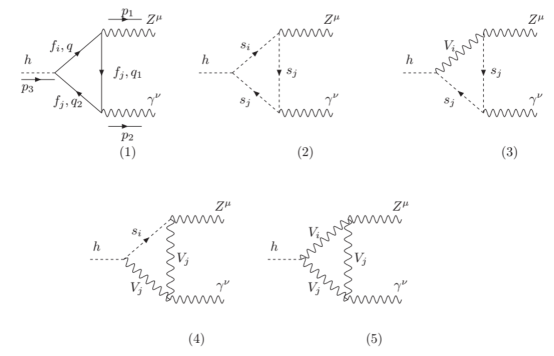
Figure 1: One-loop three-point Feynman diagrams contributing to the decay $h\rightarrow\,Z\gamma$ in the unitary gauge, where $f_{i,j}$ are the SM fermions, $s_{i,j}=H^{\pm}_{1,2},H^{\pm\pm}_{1,2}$, $V_{i,j}=W_{1}^{\pm},W_{2}^{\pm}$.

where the unitary gauge is applied to determine the gauge boson contributions. The fermion contributions to amplitude of the decay $h\to Z\gamma$ coincide with the SM results calculated in Ref. Dedes:2019bew ; Dawson:2018pyl . Using the general calculation introduced in Ref. Hue:2017cph , we can written these contribution as follows

$$F_{21,f}^{\mathrm{LR}}=F_{21,f}^{\mathrm{SM}}=\sum_{f_{i}=e_{i},u_{i},d_{i}}F_{21,f_{i}}^{\mathrm{SM}},$$ (35)

where all form factors $F_{21,f_{i}}^{\mathrm{SM}}$ are written interms of the Passrino-Veltman notations Passarino:1978jh .

Similarly, the contribution from the charged Higgs bosons can be given as

$$F^{\mathrm{LR}}_{21,S} =F_{21,H^{+}_{1}}+F_{21,H^{+}_{2}}+F_{21,H^{+}_{122}}+F_{21,H^{+}_{211}}$$

$$+F_{21,H^{++}_{1}}+F_{21,H^{++}_{2}}+F_{21,H^{++}_{122}}+F_{21,H^{++}_{211}}.$$ (36)

The charged gauge boson contributions $W^{\pm}_{1,2}$ to the $h\to Z\gamma$ amplitude are

$$F^{\mathrm{LR}}_{21,V} =F^{\mathrm{LR}}_{21,W^{+}_{1}}+F^{\mathrm{LR}}_{21,W^{+}_{2}}+F^{\mathrm{LR}}_{21,W^{+}_{122}}+F^{\mathrm{LR}}_{21,W^{+}_{211}}.$$ (37)

Similarly, the contribution from charged Higgs and gauge boson arising from two diagrams 3 and 4 in Fig. 1 can be given as

$$F^{\mathrm{LR}}_{21,VS} =F_{21,WSS}^{\mathrm{LR}}+F_{21,SWW}^{\mathrm{LR}},$$ (38)

where

$$F^{\mathrm{LR}}_{21,WSS} =F_{21,W^{+}_{1}H^{+}_{1}H^{+}_{1}}^{\mathrm{LR}}+F_{21,W^{+}_{1}H^{+}_{2}H^{+}_{2}}^{\mathrm{LR}}+F_{21,W^{+}_{2}H^{+}_{1}H^{+}_{1}}^{\mathrm{LR}}+F_{21,W^{+}_{2}H^{+}_{2}H^{+}_{2}}^{\mathrm{LR}},$$ (39)

$$F^{\mathrm{LR}}_{21,SWW} =F_{21,H^{+}_{1}W^{+}_{1}W^{+}_{1}}^{\mathrm{LR}}+F_{21,H^{+}_{1}W^{+}_{2}W^{+}_{2}}^{\mathrm{LR}}+F_{21,H^{+}_{2}W^{+}_{1}W^{+}_{1}}^{\mathrm{LR}}+F_{21,H^{+}_{2}W^{+}_{2}W^{+}_{2}}^{\mathrm{LR}}.$$ (40)

Now, the $h\to Z\gamma$ partial decay width is Gunion:1989we ; Degrande:2017naf

$$\Gamma^{\mathrm{LR}}(h\rightarrow Z\gamma)=\frac{m_{h}^{3}}{32\pi}\times\left(1-\frac{m_{Z}^{2}}{m_{h}^{2}}\right)^{3}|F^{\mathrm{LR}}_{21}|^{2},$$ (41)

where the scalar factors $F^{\mathrm{LR}}_{21}$ is derived as follows Hue:2017cph

$$F^{\mathrm{LR}}_{21} =F^{\mathrm{LR}}_{21,f}+F^{\mathrm{LR}}_{21,S}+F^{\mathrm{LR}}_{21,V}+F^{\mathrm{LR}}_{21,VS}.$$ (42)

We note that $F^{\mathrm{LR}}_{21,VS}$ were omitted in some previous works Yue:2013qba ; Martinez:1989kr ; Martinez:1990ye because it was expected to be smaller than the contributions from the SM and which is still far from the sensitivity of the recent experiments. However, since collider sensitivity has recently been improved and new scales have been established, their contribution is necessary. The branching ratio $\mathrm{Br}^{\mathrm{LR}}(h\rightarrow Z\gamma)$ in the MLRSM framework is

$$\mathrm{Br}^{\mathrm{LR}}(h\rightarrow Z\gamma)=\frac{\Gamma^{\mathrm{LR}}(h\rightarrow Z\gamma)}{\Gamma^{\mathrm{LR}}_{h}},$$ (43)

where $\Gamma^{\mathrm{LR}}_{h}$ is the total decay width of the SM-like Higgs boson $h$  Gunion:1989we ; Degrande:2017naf . Although there are available experimental measurements of the SM-like Higgs boson productions and decays Khachatryan:2016vau , we focus only on the Higgs production through the gluon fusion process $ggF$ at LHC, in which the respective signal strength predicted by two models SM and MLSM are equal. Then the signal strength corresponding to the decay mode $h\to Z\gamma$ predicted by the MLRSM is:

$$\mu_{Z\gamma}^{\mathrm{LR}}\equiv\frac{\mathrm{Br}^{\mathrm{LR}}(h\rightarrow Z\gamma)}{\mathrm{Br}^{\mathrm{SM}}(h\rightarrow Z\gamma)},$$ (44)

where $\mathrm{Br}^{\mathrm{SM}}(h\rightarrow Z\gamma)$ is the SM branching ratio of the decay $h\to Z\gamma$. The recent $ggF\to h\to Z\gamma$ singal strength is $\mu_{Z\gamma}=2.4\pm 0.9$ at $2.7\sigma$ (standard deviation) CMS:2022ahq ; CMS:2023mku .

Similarly, the partial decay width and signal strength of the decay $h\rightarrow\gamma\gamma$ can be calculated as Degrande:2017naf ; Hue:2017cph

$$\Gamma^{\mathrm{LR}}(h\rightarrow\gamma\gamma)= \frac{m_{h}^{3}}{64\pi}\times|F^{\mathrm{LR}}_{\gamma\gamma}|^{2},$$

$$\mu_{\gamma\gamma}^{\mathrm{LR}}\equiv \frac{\Gamma^{\mathrm{LR}}(h\rightarrow\gamma\gamma)}{\Gamma^{\mathrm{SM}}(h\rightarrow\gamma\gamma)},$$ (45)

where

$$F^{\mathrm{LR}}_{\gamma\gamma} =\sum_{f}F^{\mathrm{LR}}_{\gamma\gamma,f}+\sum_{s}F^{\mathrm{LR}}_{\gamma\gamma,s}+\sum_{v}F^{\mathrm{LR}}_{\gamma\gamma,v},$$ (46)

and

$$F_{\gamma\gamma,f}^{\mathrm{LR}}= F_{\gamma\gamma,f}^{\mathrm{SM}}=\sum_{f_{i}=e_{i},u_{i},d_{i}}F_{\gamma\gamma,f_{i}}^{\mathrm{SM}},$$

$$F^{\mathrm{LR}}_{\gamma\gamma,S}= F_{\gamma\gamma,H^{+}_{1}}+F_{\gamma\gamma,H^{+}_{2}}+F_{\gamma\gamma,H^{++}_{1}}+F_{\gamma\gamma,H^{++}_{2}},$$

$$F^{\mathrm{LR}}_{\gamma\gamma,V}= F_{\gamma\gamma,W^{+}_{1}}+F_{\gamma\gamma,W^{+}_{2}}.$$ (47)

Here we have used the notations that Hung:2019jue

$$F^{\mathrm{SM}}_{\gamma\gamma,f_{i}} =-\frac{e^{2}\,Q^{2}_{f_{i}}\,N_{c}}{2\pi^{2}}\left(m_{f}Y_{h\bar{f}fL}\right)\left[4X_{2}+C_{0}\right],$$

$$F_{\gamma\gamma,s} =\frac{e^{2}\,Q^{2}_{s}\lambda_{hss}}{2\pi^{2}}X_{2},$$

$$F_{\gamma\gamma,v} =\frac{e^{2}\,Q^{2}_{V}\,g_{hvv}}{4\pi^{2}}\times\left\{\left(6+\frac{m_{h}^{2}}{m_{V}^{2}}\right)X_{2}+4C_{0}\right\},$$ (48)

where $X_{2}=C_{12}+C_{22}+C_{2}$ and $C_{0,i,ij}\equiv C_{0,i,ij}(0,0,m_{h}^{2};m_{x}^{2},m_{x}^{2},m_{x}^{2})$ are Passarino-Veltman functions Passarino:1978jh with $x=f,s,v$ implying fermions, charged Higgs and gauge bosons, respectively. Particular forms given in Eq. (III.2) are defined precisely in Ref. Hung:2019jue . In the following section, the numerical results will be evaluated using LoopTools Hahn:1998yk .

IV Numerical discussions

IV.1 Setup parameters

In this section, there are following quantities fixed from experiments Tanabashi:2018oca : $m_{h}=125.38$ GeV, $m_{W}$, $m_{Z}$, well-known fermion masses, $v\simeq 246$ GeV, the $SU(2)_{L}$ gauge coupling $g_{2}\simeq 0.651$, $\alpha_{\mathrm{em}}=1/137$, $e=\sqrt{4\pi\alpha_{\mathrm{em}}}$, $s^{2}_{W}=0.231$.

The unknown independent parameters of the MLRSM used as inputs are $\beta_{1,3}$, $\rho_{1,2,3,4}$, $\alpha_{1,2,3}$, $\lambda_{1,2,3,4}$. The dependent parameters include $\lambda_{1}$ calculated by the Eq. (II.4), $\alpha_{1,2}$ and $\alpha_{4}$ calculated by the Eq. (49)

$$\alpha_{2}=\frac{\alpha_{3}t_{\beta}}{2(1-t_{\beta}^{2})},\alpha_{1}=\frac{\alpha_{3}}{t_{\beta}^{2}-1},\alpha_{4}=-\frac{2\alpha_{6}}{t_{\beta}}.$$ (49)

Higgs self-couplings are calculated through the heavy Higgs boson masses in the MLRSM, namely

$$m^{2}_{H^{0}_{1}} =m^{2}_{A_{2}}=m^{2}_{H^{\pm}_{1}}=\frac{\alpha_{3}v_{R}^{2}}{2\left(2s_{\beta}^{2}-1\right)},$$

$$m^{2}_{H^{0}_{2}} =m^{2}_{H^{\pm}_{2}}=m^{2}_{H^{\pm\pm}_{1}}=m^{2}_{A_{2}}=\frac{v_{R}^{2}}{2}\left(-2\rho_{1}+\rho_{3}\right),\;$$

$$m^{2}_{H^{0}_{3}} =2\rho_{1}v_{R}^{2},\;m^{2}_{H^{\pm\pm}_{2}}=2\rho_{2}v_{R}^{2}.$$ (50)

Choosing the mass of $m_{H^{+}_{1}}$, $m_{H^{+}_{2}}$, and $m_{H^{++}_{1}}$ as free parameters we get

$$\alpha_{1} =\frac{2m_{H_{2}^{+}}^{2}}{\left(t_{\beta}^{2}+1\right)v_{R}^{2}},\;\alpha_{2}=-\frac{t_{\beta}m_{H_{2}^{+}}^{2}}{\left(t_{\beta}^{2}+1\right)v_{R}^{2}},\;\alpha_{3}=\frac{2\left(t_{\beta}^{2}-1\right)m_{H_{2}^{+}}^{2}}{\left(t_{\beta}^{2}+1\right)v_{R}^{2}},\;$$

$$\alpha_{4} =-\frac{2\alpha_{6}}{t_{\beta}},\;\rho_{2}=\frac{m_{H_{2}^{\text{++}}}^{2}}{2v_{R}^{2}},\;\rho_{3}=2\rho_{1}+\frac{2m_{H_{1}^{+}}^{2}}{v_{R}^{2}}.$$ (51)

The other free parameters are $\lambda_{2,3,4}$, $\rho_{1}=m^{2}_{H^{0}_{3}}/(2v_{R}^{2})>0$, the mixing angle and the gauge bosons masses will be at the orders of $\mathcal{O}(v^{2}/v_{R}^{2})$

$$g_{R} =g_{L}=g_{2}=e/s_{W},\;g^{\prime}=\frac{e}{\sqrt{1-2s^{2}_{W}}},$$

$$s_{\xi} =-\frac{s_{\beta}c_{\beta}v^{2}}{v_{R}^{2}}\ll 1,\;c_{\xi}=1+\mathcal{O}\left(\frac{v^{4}}{v_{R}^{4}}\right)\simeq 1,$$

$$s_{R} =\frac{\sqrt{1-2s_{W}^{2}}}{c_{W}},\;c_{R}=t_{W},$$

$$s_{z_{2}} =s_{W},\;c_{z_{2}}=c_{W},$$

$$s_{z_{3}} =\frac{t_{W}^{2}\sqrt{1-2s_{W}^{2}}v^{2}}{4c_{W}^{2}v_{R}^{2}}\ll 1,\;c_{z_{3}}=1+\mathcal{O}\left(\frac{v^{4}}{v_{R}^{4}}\right)\simeq 1.$$ (52)

We note here that the relations given in Eq. (IV.1) are consistent with the SM because the two couplings $hW^{+}W^{-}$ and $ZW^{+}W^{-}$ are consistent with the SM predictions.

In investigating the $h\to Z\gamma$ decays, the values of unknown independent parameters we choose here will be scanned in the following ranges:

$$m_{H^{+}_{1}},\;m_{H^{+}_{2}},m_{H^{++}_{2}}\in[100,\;1000]\;\mathrm{GeV},\;v_{R}\in[1,\;10]\;\mathrm{TeV},\;t_{\beta}\in[5,50],$$

$$\lambda_{2,3,4},\alpha_{3}\in[-10,10],$$ (53)

where the Higgs self-couplings satisfy the perturbative limits, $v_{R}$ is large enough to generate the heavy gauge bosons masses satisfying the current experimental constraints, $t_{\beta}>1$ due to model survey conditions.

IV.2 Results and discussions

To express the differences of the prediction between the SM and the MLRSM, we define a quantity $\Delta\mu_{Z\gamma}$ as in Ref. Hung:2019jue

$$\Delta{\mu}^{\mathrm{LR}}_{Z\gamma}\equiv\left(\mu^{\mathrm{LR}}_{Z\gamma}-1\right)\times 100\%,$$ (54)

which is constrained by recent experiments $\Delta\mu_{Z\gamma}=1.4\pm 0.9$ CMS:2022ahq ; CMS:2023mku , implying the $1\sigma$ deviation is

$$50\%\leq\Delta{\mu}^{\mathrm{LR}}_{Z\gamma}\leq 230\%.$$ (55)

The $1\sigma$ constraint from $h\to\gamma\gamma$ decay originating from $ggF$ fusion is defined as $\Delta\mu^{\mathrm{LR}}_{\gamma\gamma}\equiv(\mu^{\mathrm{LR}}_{\gamma\gamma}-1)\times 100\%$, leading to the respective $2\sigma$ deviation is

$$-12\%<\Delta\mu^{\mathrm{LR}}_{\gamma\gamma}<38\%.$$ (56)

The numerical results we discuss in the following will always satisfy this constraint. We will focus in the region satisfying $|\Delta\mu^{\mathrm{LR}}_{Z\gamma}|\geq 10\%$ to collect interesting points that may support the $1\sigma$ range given in Eq. (55). We have checked numerically that the MLRSM always contains regions of the parameter space that both values of $\Delta{\mu}_{Z\gamma},\Delta{\mu}_{\gamma\gamma}\to 0$, implying the consistency with the SM results. Firstly, we discuss on the dependence of $\Delta\mu^{\mathrm{LR}}_{Z\gamma}$ on $\Delta\mu^{\mathrm{LR}}_{\gamma\gamma}$, which is illustrated in Fig. 2.

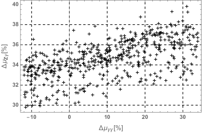
Figure 2: Correlations between $\Delta\mu_{Z\gamma}^{\mathrm{LR}}$ and $\Delta\mu_{\gamma\gamma}^{\mathrm{LR}}$.

It can be seen that $\Delta\mu_{Z\gamma}^{\mathrm{LR}}$ is constrained strictly by $\Delta\mu_{\gamma\gamma}^{\mathrm{LR}}$, i.e., $\Delta\mu_{Z\gamma}^{\mathrm{LR}}<40\%$ in the range of $2\sigma$ deviation given in  “Eq. (56)”. It is noted that negative values of $\Delta\mu_{\gamma\gamma}^{\mathrm{LR}}<0$ can give large $\Delta\mu_{Z\gamma}^{\mathrm{LR}}$ than the positive ones. But largest values of $\Delta\mu_{Z\gamma}^{\mathrm{LR}}$ is still smaller than the $1\sigma$ deviation given by recent experimental data. Therefore, in the future, if large $\Delta\mu_{Z\gamma}^{\mathrm{LR}}$ and small $\Delta\mu_{\gamma\gamma}^{\mathrm{LR}}$ are confirmed experimentally, the assumption given in Eq. (IV.1) must be changed.

We comment here a point that the future sensitivities are $|\Delta\mu_{\gamma\gamma}|\leq 4\%$, and $|\Delta\mu_{Z\gamma}|\leq 23\%$, respectively Cepeda:2019klc . In the model under consideration, large values of $\Delta\mu_{Z\gamma}>23\%$ are still allowed in the very strict constraint from $\Delta\mu_{\gamma\gamma}$.

Now, we discuss on the dependence of $\Delta\mu^{\mathrm{LR}}_{Z\gamma}$ on $t_{\beta}$ and $v_{R}$, which are shown in Fig. 3.

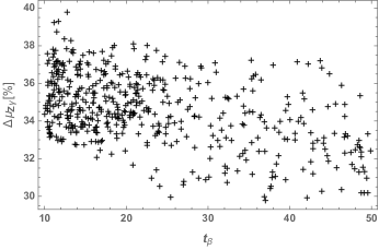
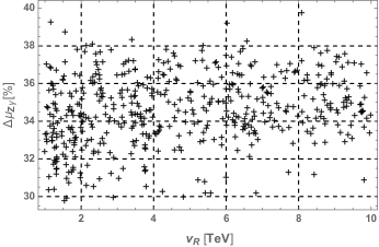
Figure 3: Correlations between $\Delta\mu_{Z\gamma}^{\mathrm{LR}}$ with different values of $t_{\beta}$ and $v_{R}$.

We can see that $\Delta\mu_{Z\gamma}^{\mathrm{LR}}$ depends weakly on these two parameters. Namely, all values of $t_{\beta}$ and $v_{R}$ can give large $\Delta\mu_{Z\gamma}^{\mathrm{LR}}>35\%$.

The correlations between $\Delta\mu_{Z\gamma}^{\mathrm{LR}}$ and charged Higgs boson masses are shown in Fig. 4.

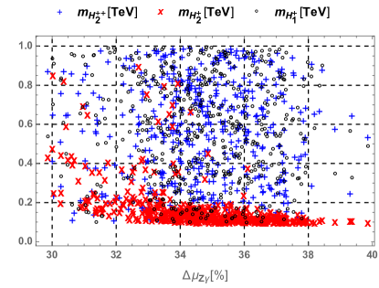
Figure 4: Correlations between $\Delta\mu_{Z\gamma}^{\mathrm{LR}}$ and charged Higgs bosons masses $m_{H^{\pm\pm}_{1}}$ and $m_{H^{\pm}_{1,2}}$.

The results show that only $m_{H^{\pm}_{1}}$ gives large $\Delta\mu^{\mathrm{LR}}_{Z\gamma}$, i.e. $m_{H^{\pm}_{1}}<200$ GeV for $\Delta\mu^{\mathrm{LR}}_{Z\gamma}>37\%$. In contrast, the other masses do not affect strongly on values of $\Delta\mu^{\mathrm{LR}}_{Z\gamma}$.

V Conclusions

We have studied all one-loop contributions to the SM-like Higgs decays $h\to\gamma\gamma,Z\gamma$ in the MLRSM framework. Interesting properties of the new gauge and Higgs bosons were explored. Namely, the SM-like Higgs couplings were identified with the SM prediction and experimental data. All masses, physical states of gauge and Higgs bosons, and their mixing were presented clearly so that all couplings relate to one-loop contributions the decay amplitudes $h\to\gamma\gamma,Z\gamma$ are derived analytically. From this, decays $h\rightarrow\gamma\gamma,Z\gamma$ in MLRSM have been discussed using the relevant recent experimental results. The one-loop contributions from the diagrams containing both gauge and Higgs mediation were included in the decay amplitude $h\rightarrow Z\gamma$. These contributions were ignored in previous studies, although they may enhance the $h\rightarrow Z\gamma$ amplitude, but do not affect the $h\rightarrow\gamma\gamma$ one, leading to the possibility that large $\Delta\mu_{Z\gamma}$ may be allowed under the strict experimental constraint of $\Delta\mu_{\gamma\gamma}$. We have shown that the mentioned $h$ decay rates depend weakly on $t_{\beta}$, the $SU(2)_{R}$ vacuum scale $v_{R}$. The $2\sigma$ deviation of $\mu_{\gamma\gamma}$ results in a rather strict constraint $\left|\Delta\mu_{Z\gamma}\right|<40\%$. On the other hand, the large values of $\Delta\mu_{Z\gamma}>23\%$ can appear under the very strict constraint of $|\Delta\mu_{\gamma\gamma}|\leq 4\%$ corresponding to the future experimental sensitivities. Therefore, the future experimental searches of the two decays mentioned in this work will be important to constrain the parameter space of the MLRSM.

References

- (1) A. Tumasyan et al. [CMS], Nature 607, no.7917, 60-68 (2022) [arXiv:2207.00043 [hep-ex]].
- (2) A. Tumasyan et al. [CMS], JHEP 05, 233 (2023) [arXiv:2204.12945 [hep-ex]].
- (3) G. Aad et al. [CMS and ATLAS], [arXiv:2309.03501 [hep-ex]].
- (4) A. M. Sirunyan et al. [CMS], JHEP 07, 027 (2021) [arXiv:2103.06956 [hep-ex]].
- (5) C. X. Yue, Q. Y. Shi and T. Hua, Nucl. Phys. B 876 (2013) 747 [arXiv:1307.5572 [hep-ph]].
- (6) H. T. Hung, T. T. Hong, H. H. Phuong, H. L. T. Mai and L. T. Hue, Phys. Rev. D 100 (2019) no.7, 075014 [arXiv:1907.06735 [hep-ph]].
- (7) D. Fontes, J. C. Romão and J. P. Silva, JHEP 12, 043 (2014) [arXiv:1408.2534 [hep-ph]].
- (8) E. Yildirim, Int. J. Mod. Phys. A 37 (2022) no.13, 2250067 [arXiv:2112.06836 [hep-ph]].
- (9) R. Benbrik, M. Boukidi, M. Ouchemhou, L. Rahili and O. Tibssirte, Nucl. Phys. B 990 (2023), 116154 [arXiv:2211.12546 [hep-ph]].
- (10) L. T. Hue, D. T. Tran, T. H. Nguyen and K. H. Phan, PTEP 2023, no.8, 083B06 (2023) [arXiv:2305.04002 [hep-ph]].
- (11) X. Wang, S. M. Zhao, T. T. Wang, L. H. Su, W. Li, Z. N. Zhang, Z. J. Yang and T. F. Feng, Eur. Phys. J. C 82, no.11, 977 (2022) [arXiv:2205.14880 [hep-ph]].
- (12) D. T. Tran, T. H. Nguyen and K. H. Phan, [arXiv:2311.02998 [hep-ph]].
- (13) P. Archer-Smith, D. Stolarski and R. Vega-Morales, JHEP 10 (2021), 247 [arXiv:2012.01440 [hep-ph]].
- (14) C. X. Liu, H. B. Zhang, J. L. Yang, S. M. Zhao, Y. B. Liu and T. F. Feng, JHEP 04 (2020), 002 [arXiv:2002.04370 [hep-ph]].
- (15) R. Martinez, M. A. Perez and J. J. Toscano, Phys. Lett. B 234 (1990), 503-507
- (16) R. Martinez and M. A. Perez, Nucl. Phys. B 347 (1990), 105-119 doi:10.1016/0550-3213(90)90553-P
- (17) M. Aaboud et al. [ATLAS Collaboration], Phys. Lett. B 786 (2018) 114 [arXiv:1805.10197 [hep-ex]].
- (18) A. M. Sirunyan et al. [CMS Collaboration], JHEP 1811 (2018) 185 [arXiv:1804.02716 [hep-ex]].
- (19) M. Aaboud et al. [ATLAS Collaboration], Phys. Rev. D 98 (2018) 052005 [arXiv:1802.04146 [hep-ex]].
- (20) M. Aaboud et al. [ATLAS Collaboration], JHEP 1710 (2017) 112 [arXiv:1708.00212 [hep-ex]].
- (21) M. Cepeda, S. Gori, P. Ilten, M. Kado, F. Riva, R. Abdul Khalek, A. Aboubrahim, J. Alimena, S. Alioli and A. Alves, et al. CERN Yellow Rep. Monogr. 7 (2019), 221-584 [arXiv:1902.00134 [hep-ph]].
- (22) F. An, Y. Bai, C. Chen, X. Chen, Z. Chen, J. Guimaraes da Costa, Z. Cui, Y. Fang, C. Fu and J. Gao, et al. Chin. Phys. C 43 (2019) no.4, 043002 [arXiv:1810.09037 [hep-ex]].
- (23) E. S. Antonov and A. G. Drutskoy, JETP Lett. 117 (2023) no.3, 177-183 [arXiv:2212.07889 [hep-ex]].
- (24) J. C. Pati and A. Salam, Phys. Rev. D 10 (1974), 275-289 [erratum: Phys. Rev. D 11 (1975), 703-703]
- (25) R. N. Mohapatra and J. C. Pati, Phys. Rev. D 11 (1975), 2558
- (26) G. Senjanovic and R. N. Mohapatra, Phys. Rev. D 12 (1975), 1502
- (27) Y. Zhang, H. An, X. Ji and R. N. Mohapatra, Nucl. Phys. B 802, 247-279 (2008) [arXiv:0712.4218 [hep-ph]].
- (28) C. H. Lee,“Left-right symmetric model and its TeV-scale phenomenology,” doi:10.13016/M26W9693V,
- (29) A. Dedes, K. Suxho and L. Trifyllis, JHEP 06, 115 (2019) [arXiv:1903.12046 [hep-ph]].
- (30) S. Dawson and P. P. Giardino, Phys. Rev. D 97 (2018) no.9, 093003 [arXiv:1801.01136 [hep-ph]].
- (31) L. T. Hue, H. N. Long, V. H. Binh, H. L. T. Mai and T. P. Nguyen, Nucl. Phys. B 992 (2023), 116244 [arXiv:2301.05407 [hep-ph]].
- (32) L. T. Hue, A. B. Arbuzov, T. T. Hong, T. P. Nguyen, D. T. Si and H. N. Long, Eur. Phys. J. C 78 (2018) no.11, 885 [arXiv:1712.05234 [hep-ph]].
- (33) G. Passarino and M. J. G. Veltman, Nucl. Phys. B 160 (1979) 151.
- (34) J. F. Gunion, H. E. Haber, G. L. Kane and S. Dawson, “The Higgs Hunter’s Guide,” Front. Phys. 80 (2000).
- (35) C. Degrande, K. Hartling and H. E. Logan, Phys. Rev. D 96 (2017) no.7, 075013 Erratum: [Phys. Rev. D 98 (2018) no.1, 019901] [arXiv:1708.08753 [hep-ph]].
- (36) G. Aad et al. [ATLAS and CMS Collaborations], JHEP 1608 (2016) 045 [arXiv:1606.02266 [hep-ex]].
- (37) T. Hahn and M. Perez-Victoria, Comput. Phys. Commun. 118 (1999) 153 [hep-ph/9807565].
- (38) M. Tanabashi et al. [Particle Data Group], Phys. Rev. D 98 (2018) no.3, 030001.