Partial Label Learning with a Partner

Abstract

In partial label learning (PLL), each instance is associated with a set of candidate labels among which only one is ground-truth. The majority of the existing works focuses on constructing robust classifiers to estimate the labeling confidence of candidate labels in order to identify the correct one. However, these methods usually struggle to rectify mislabeled samples. To help existing PLL methods identify and rectify mislabeled samples, in this paper, we introduce a novel partner classifier and propose a novel “mutual supervision” paradigm. Specifically, we instantiate the partner classifier predicated on the implicit fact that non-candidate labels of a sample should not be assigned to it, which is inherently accurate and has not been fully investigated in PLL. Furthermore, a novel collaborative term is formulated to link the base classifier and the partner one. During each stage of mutual supervision, both classifiers will blur each other’s predictions through a blurring mechanism to prevent overconfidence in a specific label. Extensive experiments demonstrate that the performance and disambiguation ability of several well-established stand-alone and deep-learning based PLL approaches can be significantly improved by coupling with this learning paradigm.

Introduction

As a representative framework of weakly supervised learning, partial label learning (PLL), where each instance is associated with a set of candidate labels among which only one is ground-truth, has garnered increasing attention in recent years (Cour, Sapp, and Taskar 2011; Han et al. 2018; Jin and Ghahramani 2002a; Papandreou et al. 2015; Ren et al. 2018; Zhou 2018; Zhu and Goldberg 2009; Chai, Tsang, and Chen 2020; Ren et al. 2018; Li, Guo, and Zhou 2021; Li and Liang 2019). PLL has also been applied to many real-world applications due to the growing demand for identifying the valid label from a set of candidate labels. For instance, in the automatic face naming task (Zeng et al. 2013; Guillaumin, Verbeek, and Schmid 2010), each face crapped from images or videos is associated with a list of names extracted from the corresponding title or caption (Gong, Yuan, and Bao 2022). Another example is the facial age estimation task: for each human face, the ages annotated by crowd-sourcing labelers are considered as candidate labels (Panis et al. 2016).

Formally speaking, suppose $\mathcal{X}=\mathbb{R}^{q}$ denotes the $q$-dimensional feature space and let $\mathcal{Y}=\{0,1\}^{l}$ be the label space with $l$ classes. Given a partial label data set $\mathcal{D}=\{\mathbf{x}_{i},S_{i}|1\leq i\leq n\}$ where $\mathbf{x}_{i}\in\mathcal{X}$, $S_{i}\subseteq\mathcal{Y}$ is the corresponding candidate label set and $n$ is the number of instances, the task of PLL is to induce a multi-class classifier $f:\mathcal{X}\rightarrow\mathcal{Y}$ based on $\mathcal{D}$. The most challenging part of PLL is that the ground-truth label $y_{i}$ of a training sample $\mathbf{x}_{i}$ conceals in its candidate labels, i.e, $y_{i}\in S_{i}$, which cannot be directly accessible during the training process.

To address this challenge, existing works focus on disambiguation, which involves differentiating the labeling confidences of each candidate label to identify the ground truth. This process typically relies on an alternative and iterative method for updating the classifier’s parameters. For instance, PL-AGGD (Wang, Zhang, and Li 2022) constructs a similarity graph to achieve disambiguation, and SURE (Feng and An 2019) aims to maximize an infinity norm to differentiate the ground-truth label. However, a significant yet rarely studied question arises in the context of such algorithms: can a classifier correct a false positive candidate label (i.e., invalid candidate label) with a large or upward-trending labeling confidence at a later stage? To explore this question, we conduct experiments on a real-world data set Lost (Cour et al. 2009) and record the labeling confidences of several candidate labels generated by PL-AGGD (Wang, Zhang, and Li 2022) in each iteration, which is shown in Fig. 1. Our findings reveal some intriguing phenomena:

• Each candidate label’s labeling confidence is likely to continually increase or decrease until convergence.

• For a false positive candidate label with a large labeling confidence, although its confidence may decrease in subsequent iterations, the confidence remains substantial and can easily lead to the incorrect identification of the ground truth label.

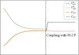
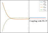
Figure 1: Two representative errors a typical PLL classifier, e.g., PL-AGGD (Wang, Zhang, and Li 2022) may make. $C_{GT}$ and $C_{GT}^{*}$ stand for the labeling confidence of the ground-truth label generated by PL-AGGD and PL-AGGD coupled with PLCP, and $C_{FP}$ and $C_{FP}^{*}$ stand for that of a false positive label predicted by PL-AGGD and PL-AGGD coupled with PLCP. (a). For a false positive candidate label with a large labeling confidence, although its confidence may decrease properly, it could still be larger than the ground-truth one’s. (b). The labeling confidence of a false positive candidate label keeps increasing and becomes the largest, which misleads the final prediction. When coupled with PLCP (vertical dashed line), the new labeling confidence of each candidate label generated by the partner classifier is adopted as the supervision to help PL-AGGD correct these errors, which results in a mutation in the figures.

The observed phenomena suggest that once the labeling confidence of a false positive candidate label increases, it becomes difficult to decrease in the subsequent iterations. Furthermore, even if the confidence of a false positive candidate label decreases appropriately, it may still be recognized as the ground truth one, as its initial labeling confidence remains large and continues to be greater than the confidence of the ground truth label upon convergence. As a result, correcting mislabeled samples for a PLL classifier itself proves to be quite challenging.

To address the aforementioned challenge, we propose a novel PLL mutual supervision framework called PLCP, referring to Partial Label Learning with a Classifier as Partner. Given a classifier provided by any existing PLL approach as the base classifier, as shown in Fig. 2, PLCP introduces an additional partner classifier to help the base classifier identify and rectify mislabeled samples. This partner classifier aims to provide more accurate and complementary information to the base classifier, thereby enabling better disambiguation and facilitating mutual supervision between the two classifiers. It is worth noting that the design of an effective partner classifier is crucial to the success of this framework, as the feedback from the partner classifier greatly influences the base classifier’s ability to identify and correct mislabeled samples. Since the information in non-candidate labels, which indicates that a set of labels DO NOT belong to a sample, is more precise than that in candidate labels and is often overlooked by the majority of existing works, the partner classifier can be designed to specify the labels that should not be assigned to a sample, thereby complementing the base classifier. Additionally, a novel collaborative term is also designed to link the base classifier and the partner classifier.

In each stage of mutual supervision, the labeling confidence is first updated based on the base classifier’s modeling output. Subsequently, a blurring mechanism is employed to further process the labeling confidence to introduce uncertainty, which could potentially reduce the large confidence of some false positive candidate labels or increase the small confidence of the ground truth one. This updated labeling confidence then serves as the supervision information to interact with the partner classifier, whose final output will also be converted to supervise the base classifier. The predictions of the two classifiers, while distinct, are inextricably linked, enhancing the disambiguation ability of this paradigm in two opposing ways. With this mutual supervision paradigm, mislabeled instances have a higher likelihood of being corrected.

The main contributions of this paper can be summarized as follows:

• We highlight two representative errors that a PLL classifier may make, which has not been previously investigated and offers a new insight into PLL.

• We introduce a partner classifier based on non-candidate labels to better identify and correct mislabeled samples of a base classifier through a mutual supervision framework, which is applicable to all types of PLL approaches.

• We propose a novel collaborative term in the partner classifier, which links the base classifier and itself. Additionally, a blurring mechanism is introduced to add uncertainty to the outputs, which effectively tackles the mentioned drawbacks.

• We conduct experiments on several data sets to validate the effectiveness of this framework, and the results demonstrate that PLCP improves the disambiguation ability of the base classifier, leading to outstanding performance across all data sets.

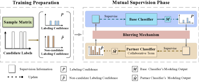
Figure 2: The framework of PLCP. A partner classifier is constructed based on the non-candidate label information to enable mutual supervision between the base classifier and itself. In each stage of mutual supervision, the base classifier updates the labeling confidence $\mathbf{P}$ based on its modeling output $\mathbf{M}$ and blurs it through a blurring mechanism. Afterwards, the output is represented as the supervision information to interact with the partner classifier. The pipeline of the partner classifier is almost the same as the base classifier’s.

Related Work

Partial Label Learning

Partial label learning (PLL), also known as superset-label learning (Liu and Dietterich 2012, 2014) or ambiguous label learning (Hüllermeier and Beringer 2005; Zeng et al. 2013), is a representative weakly supervised learning framework which learns from inaccurate supervision information. In partial label learning, each instance is associated with a set of candidate labels with only one being ground-truth and others being false positive. As the ground-truth label of a sample conceals in the corresponding candidate label set, which can not be directly acquired during the training process, partial label learning task is a quite challenging problem.

To tackle the mentioned challenge, existing works mainly focus on disambiguation (Feng and An 2019; Nguyen and Caruana 2008; Zhang and Yu 2015; Wang, Zhang, and Li 2022; Fan et al. 2021; Xu, Lv, and Geng 2019; Zhang, Wu, and Bao 2022; Qian et al. 2023), which can be broadly divided into two categories: averaging-based approaches and identification-based approaches. For the averaging-based approaches (Hüllermeier and Beringer 2005; Cour, Sapp, and Taskar 2011; Zhang and Yu 2015), each candidate label of a training sample is treated equally as the ground-truth one and the final prediction is yielded by averaging the modeling outputs. For instance, PL-KNN (Hüllermeier and Beringer 2005) averages the candidate labels of neighboring samples to make the prediction. This kind of approach is intuitive, however, it can be easily influenced by false positive candidate labels which results in inferior performance. For identification-based approaches, (Feng and An 2018, 2019; Nguyen and Caruana 2008; Jin and Ghahramani 2002b; Yu and Zhang 2017), the ground-truth label is treated as a latent variable and can be identified through an iterative optimization procedure such as EM. Moreover, labeling confidence based strategy is proposed in many state-of-the-art identification based approaches for better disambiguation. (Zhang and Yu 2015) and (Wang, Zhang, and Li 2022) construct a similarity graph based on the feature space to generate labeling confidence of candidate labels.

Recently, deep-learning based models have been introduced to address PLL tasks (Lv et al. 2020; Xu et al. 2021; He et al. 2022; Wu, Wang, and Zhang 2022; Lyu, Wu, and Feng 2022; Xia et al. 2023). PICO (Wang et al. 2022) is a contrastive learning-based approach devised to tackle label ambiguity in partial label learning. This method seeks to discern the ground-truth label from the candidate set by utilizing contrastively learned embedding prototypes. Lv et al. proposed PRODEN in (Lv et al. 2020), a model where the simultaneous updating of the model and identification of true labels are seamlessly integrated. Furthermore, He et al. introduced a partial label learning method based on semantic label representations in (He et al. 2022). This method employs a novel weighted calibration rank loss to facilitate label disambiguation. By leveraging label confidence, the approach weights the similarity towards all candidate labels and subsequently yields a higher similarity of candidate labels in comparison to each non-candidate label.

However, as mentioned in Section 1, the above kinds of approach usually fail to identify and correct the mislabeled samples. to address this challenge, we propose a novel framework called PLCP in the next section.

Learning from Non-candidate Labels

The utilization of non-candidate labels (a.k.a. complementary labels) is not a novel concept. Earlier studies on complementary-label learning (CLL) (Ishida et al. 2017, 2019; Gao and Zhang 2021; Katsura and Uchida 2020) centered around classification tasks involving one single complementary label. In contrast to CLL, our approach involves the generation of complementary labels derived from non-candidate labels, serving the purpose of disambiguation in PLL.

The Proposed Approach

Denote $\mathbf{X}=[\mathbf{x}_{1},\mathbf{x}_{2},...,\mathbf{x}_{n}]^{\mathsf{T}}\in\mathbb{R}^{n\times q}$ the sample matrix with $n$ instances, and $\mathbf{Y}=[\mathbf{y}_{1},\mathbf{y_{2}},...,\mathbf{y}_{n}]^{\mathsf{T}}\in\{0,1\}^{n\times l}$ the partial label matrix with $l$ labels, where $y_{ij}=1$ (resp. $y_{ij}=0$) if the $j$-th label of $\mathbf{x}_{i}$ resides in (resp. does not reside in) its candidate label set. Given the partial label data set $\mathcal{D}=\{\mathbf{x}_{i},S_{i}|1\leq i\leq n\}$, the task of PLL is to learn a multi-class classifier $f:\mathcal{X}\rightarrow\mathcal{Y}$ based on $\mathcal{D}$.

To address the challenge described in Section 1, a partner classifier $\mathcal{P}$ is designed to complement a base classifier $\mathcal{B}$ and also can be supervised by $\mathcal{B}$. $\mathcal{B}$ represents any existing PLL classifier with fine generality and flexibility. In each stage of mutual supervision, the base classifier updates the labeling confidence based on its modeling outputs, and then a blurring mechanism is applied to further process it. Subsequently the output of the labeling confidence is taken as the supervision information for the partner classifier. The learning pipeline of the partner classifier closely mirrors that of the base classifier. The following subsections will provide further details on this process.

Base Classifier

Suppose $\mathbf{P}=[\mathbf{p}_{1},\mathbf{p}_{2},...,\mathbf{p}_{n}]^{\mathsf{T}}\in\mathbb{R}^{n\times l}$ is the labeling confidence matrix, where $\mathbf{p}_{i}\in\mathbb{R}^{l}$ represents the labeling confidence vector of $\mathbf{x}_{i}$, and $p_{ij}$ denotes the probability of the $j$-th label being the ground-truth label of $\mathbf{x}_{i}$. For the base classifier utilizing the labeling confidence strategy, $\mathbf{P}$ is initialized according to the base classifier. Otherwise, it is initialized as follows:

$$p_{ij}=\left\{\begin{array}[]{ll}\frac{1}{\sum_{j}y_{ij}}&\text{ if }\quad y_{ij}=1\\ 0&\text{ otherwise }.\end{array}\right.$$ (1)

The labeling confidence vector $\mathbf{p}_{i}$ typically satisfies the following constraints: $\sum_{j}p_{ij}=1$, $0\leq p_{ij}\leq y_{ij}$ (Wang, Zhang, and Li 2022; Feng and An 2018). The first constrains $\mathbf{p}_{i}$ to be normalized, and the second indicates that only the confidence of a candidate label has a chance to be positive. It should be noted that the ideal state of $\mathbf{p}_{i}$ is one-hot.

Once the base classifier has been trained, its modeling output will be generated. Denote the modeling output matrix $\mathbf{M}=[\mathbf{m}_{1},\mathbf{m}_{2},...,\mathbf{m}_{n}]^{\mathsf{T}}\in\mathbb{R}^{n\times l}$, where $\mathbf{m}_{ij}$ represents the probability of the $j$-th label being $\mathbf{x}_{i}$’s ground-truth label as predicted by the base classifier. It should be noted that $\mathbf{m}_{i}$ may either be a real-valued or one-hot vector depending on the specific base classifier. For instance, for SURE (Feng and An 2019) $\mathbf{m}_{i}$ is real-valued, while for PL-KNN (Hüllermeier and Beringer 2005) it is one-hot. Afterwards, $\mathbf{P}$ is updated to $\mathbf{P}_{1}$ through the following equation:

$$\mathbf{P}_{1}=\mathcal{T}_{0}\left(\mathcal{T}_{\mathbf{Y}}\left(\alpha\mathbf{P}+(1-\alpha)\mathbf{M}\right)\right),$$ (2)

where $\alpha$ is a hyper-parameter controlling the smoothness of the labeling confidence. $\mathcal{T}_{0}$, $\mathcal{T}_{{\mathbf{Y}}}$ are two thresholding operators in element-wise, i.e., $\mathcal{T}_{0}(a):=\max\{0,a\}$ with $a$ being a scalar and $\mathcal{T}_{{\mathbf{Y}}}(a):=\min\{{y}_{ij},a\}$.

Blurring Mechanism

In the next step, a blurring mechanism is designed to further process the labeling confidence matrix $\mathbf{P}_{1}$ to $\mathbf{Q}_{1}$ :

$$\mathbf{Q}_{1}=\phi(e^{k}\mathbf{P}_{1})\odot\mathbf{Y},$$ (3)

where $\phi(\cdot)$ is an element-wise operator, for a matrix $\mathbf{A}=[a_{ij}]_{n\times l}\in\mathbb{R}^{n\times l}$, $\phi(\mathbf{A})=[{\rm exp}(a_{ij})]_{n\times l}$. $k$ is a temperature parameter that controls the extent of blurring of labeling confidence. The labeling confidences are expected to be blurred at each stage of mutual supervision to prevent being overconfident in some false positive labels, hence we set $k<0$, which means two labeling confidences that differ significantly can also become close. $\odot$ represents the Hadamard product of two matrices. For matrices $\mathbf{A}$ and $\mathbf{B}$ with same size $n\times l$, $\mathbf{A}\odot\mathbf{B}=[a_{ij}b_{ij}]_{n\times l}$. The Hadamard product allows only the candidate label has a positive confidence. We then normalize each row of $\mathbf{Q}_{1}$ to satisfy the two constraints of labeling confidence, and output the result $\mathbf{O}_{1}\in\mathbb{R}^{n\times l}$.

Partner Classifier

Since the partner classifier has significant impacts on the success of PLCP, designing an appropriate partner classifier is quite important. In order to better assist the base classifier, a classifier that specifies the labels that should not be assigned to a sample is instantiated as the partner classifier, since non-candidate label information is exactly accurate and opposite to the candidate label information, making it a valuable complement to the base classifier.

Denote the non-candidate label matrix $\hat{\mathbf{Y}}=[\hat{y}_{ij}]_{n\times l}$ where $\hat{y}_{ij}=0$ (resp. $\hat{y}_{ij}=1$) if the $j$-th label is (resp. is not) in the candidate label set of $\mathbf{x}_{i}$, and $\hat{\mathbf{P}}=[\hat{\mathbf{p}}_{1},\hat{\mathbf{p}}_{2},...,\hat{\mathbf{p}}_{n}]^{\mathsf{T}}\in\mathbb{R}^{n\times l}$ the non-candidate labeling confidence matrix, where $\hat{p}_{ij}$ represents the probability of the $j$-th label NOT being the ground-truth label of $\mathbf{x}_{i}$. Similar to the labeling confidence, $\hat{\mathbf{P}}$ is also constrained with two constraints: $\sum_{j}\hat{{p}}_{ij}=l-1,\hat{y}_{ij}\leq\hat{p}_{ij}\leq 1$. The first term constrains the sum of the probability of each label being invalid is strictly $l-1$, and the second indicates that only candidate label has a chance to update its non-candidate labeling confidence while the others keep 1 (invalid labels). Note that the ideal state of $\hat{\mathbf{p}}_{i}$ is “zero-hot”, i.e., only one element in $\hat{\mathbf{p}}_{i}$ is 0 with others 1. $\hat{\mathbf{P}}$ is initialized as $\hat{\mathbf{Y}}$. Suppose $\hat{\mathbf{W}}=[\hat{\mathbf{w}}_{1},\hat{\mathbf{w}}_{2},...,\hat{\mathbf{w}}_{q}]^{\mathsf{T}}\in\mathbb{R}^{q\times l}$ is the weight matrix, the partner classifier is formulated as follows:

$$\begin{split}\min_{\hat{\mathbf{W}},\hat{\mathbf{b}},\mathbf{C}}&\quad\left\|\mathbf{X}\hat{\mathbf{W}}+\mathbf{1}_{n}\hat{\mathbf{b}}^{\mathsf{T}}-\mathbf{C}\right\|_{F}^{2}+\lambda\left\|\hat{\mathbf{W}}\right\|_{F}^{2}\\ {\rm s.t.}&\quad\hat{\mathbf{Y}}\leq\mathbf{C}\leq\mathbf{1}_{n\times l},\mathbf{C}\mathbf{1}_{l}=(l-1)\mathbf{1}_{n},\end{split}$$ (4)

where $\hat{\mathbf{b}}=[\hat{b}_{1},\hat{b}_{2},...,\hat{b}_{l}]^{\mathsf{T}}\in\mathbb{R}^{l}$ is the bias term, $\mathbf{1}_{n}\in\mathbb{R}^{n}$ is an all one vectors, $\mathbf{1}_{n\times l}$ is an all one matrix with size $n\times l$ and $\lambda$ is a hyper-parameter trading off these terms. $\|\hat{\mathbf{W}}\|_{F}$ is the Frobenius norm of the weight matrix. $\mathbf{C}\in\mathbb{R}^{n\times l}$ represents non-candidate labeling confidence, which is a temporary variable only used for optimization in the partner classifier. By solving this optimization problem, the partner classifier learns to specify which labels should not be assigned to each sample, improving the overall performance of the mutual supervision process.

The Collaborative Term

Since a label is either ground-truth or not and based on the constraints on $\mathbf{p}_{i}$ and $\hat{\mathbf{p}}_{i}$, the smallest value of $\mathbf{p}_{i}^{\mathsf{T}}\hat{\mathbf{p}}_{i}$ is obtained when $\hat{\mathbf{p}}_{i}$ is zero-hot ($\mathbf{p}_{i}$ is one-hot). Therefore, a collaborative relationship between the outputs of the partner classifier and the prior given by the base classifier can be formulated, with the partner classifier becoming

$$\min_{\hat{\mathbf{W}},\hat{\mathbf{b}},\mathbf{C}} \quad\left\|\mathbf{X}\hat{\mathbf{W}}+\mathbf{1}_{n}\hat{\mathbf{b}}^{\mathsf{T}}-\mathbf{C}\right\|_{F}^{2}+\gamma{\rm tr}\left(\mathbf{O}_{1}\mathbf{C}^{\mathsf{T}}\right)+\lambda\left\|\hat{\mathbf{W}}\right\|_{F}^{2}$$

$${\rm s.t.} \quad\hat{\mathbf{Y}}\leq\mathbf{C}\leq\mathbf{1}_{n\times l},\mathbf{C}\mathbf{1}_{l}=(l-1)\mathbf{1}_{n},$$ (5)

where $\gamma$ is a hyper-parameter. Different from candidate labels, the non-candidate labels are directly accessible and accurate, therefore the information learnt by the partner classifier is precise, which can effectively complement the base classifier.

The problem in Eq. (5) can be solved via an alternative and iterative manner, which results in an optimal weight matrix $\hat{\mathbf{W}}$ and bias term $\hat{\mathbf{b}}$. For detailed solution process, please refer to the Supplementary. The modeling output $\hat{\mathbf{M}}$ for the training data is

$$\hat{\mathbf{M}}=\mathbf{X}\hat{\mathbf{W}}+\mathbf{1}_{n}\hat{\mathbf{b}}^{\mathsf{T}}.$$ (6)

Afterwards, the non-candidate labeling confidence $\hat{\mathbf{P}}$ is updated to $\hat{\mathbf{P}}_{1}$ following

$$\hat{\mathbf{P}}_{1}=\mathcal{T}_{1}\left(\mathcal{T}_{\mathbf{\hat{Y}}}\left(\alpha\hat{\mathbf{P}}+(1-\alpha)\hat{\mathbf{M}}\right)\right),$$ (7)

where $\mathcal{T}_{1}$, $\mathcal{T}_{\hat{\mathbf{Y}}}$ are two thresholding operators in element-wise, i.e., $\mathcal{T}_{1}(m):=\min\{1,m\}$ with $m$ being a scalar and $\mathcal{T}_{\hat{\mathbf{Y}}}(m):=\max\{\hat{{y}}_{ij},m\}$. The non-candidate labeling confidence can be further processed as $\hat{\mathbf{Q}}_{1}$ via the blurring mechanism:

$$\hat{\mathbf{Q}}_{1}=\phi(e^{k}(1-\hat{\mathbf{P}}_{1}))\odot\mathbf{Y}.$$ (8)

For convenience, we transform the non-candidate labeling confidence into labeling confidence in advance, and finally $\hat{\mathbf{Q}}_{1}$ is normalized as $\hat{\mathbf{O}}_{1}$, which is the supervision of the base classifier in the next iteration. For an unseen sample $\mathbf{x}$, suppose the non-candidate labeling confidence vector predicted by the partner classifier in the last iteration is $\hat{\mathbf{p}}^{pt}$. The prediction $y^{\ast}$ of PLCP is

$$y^{\ast}={\rm argmax}_{i}\quad(1-\hat{{p}}^{pt}_{i}),$$ (9)

Extensions of PLCP

We can also extend PLCP to a kernel version which extends the feature map to a higher dimensional space or a deep-learning based version which enables deep-learning based methods involved in PLCP. For more details, please refer to the Supplementary.

Experiments

Compared Approaches

To evaluate the effectiveness of PLCP, we couple it with several well-established partial label learning approaches. Suppose $\mathcal{B}$ represents any partial label learning classifier (i.e., the base classifier) and $\mathcal{B}$-PLCP is the $\mathcal{B}$ coupled with PLCP, the performances of $\mathcal{B}$ and $\mathcal{B}$-PLCP are compared to verify the effectiveness of PLCP. In this paper, $\mathcal{B}$ is instantiated by six stand-alone (non-deep) approaches, PL-CL(Jia, Si, and Zhang 2023), PL-AGGD (Wang, Zhang, and Li 2022), SURE (Feng and An 2019), LALO (Feng and An 2018), PL-SVM (Nguyen and Caruana 2008) and PL-KNN (Hüllermeier and Beringer 2005), and two deep-learning based methods PICO (Wang et al. 2022) and PRODEN (Lv et al. 2020). The hyper-parameters of $\mathcal{B}$ are all set according to the original papers.

Approaches	Data set
	FG-NET	Lost	MSRCv2	Mirflickr	Soccer Player	Yahoo!News
PL-CL	0.072 $\pm$ 0.009	0.710 $\pm$ 0.022	0.469 $\pm$ 0.016	0.647 $\pm$ 0.012	0.534 $\pm$ 0.004	0.618 $\pm$ 0.003
PL-CL-PLCP	0.080 $\pm$ 0.009 $\bullet$	0.763 $\pm$ 0.020 $\bullet$	0.493 $\pm$ 0.013 $\bullet$	0.665 $\pm$ 0.011 $\bullet$	0.543 $\pm$ 0.002 $\bullet$	0.625 $\pm$ 0.002 $\bullet$
PL-AGGD	0.063 $\pm$ 0.010	0.690 $\pm$ 0.020	0.451 $\pm$ 0.023	0.610 $\pm$ 0.012	0.521 $\pm$ 0.004	0.605 $\pm$ 0.002
PL-AGGD-PLCP	0.076 $\pm$ 0.010 $\bullet$	0.717 $\pm$ 0.020 $\bullet$	0.473 $\pm$ 0.017 $\bullet$	0.668 $\pm$ 0.014 $\bullet$	0.534 $\pm$ 0.005 $\bullet$	0.609 $\pm$ 0.002 $\bullet$
SURE	0.052 $\pm$ 0.007	0.709 $\pm$ 0.022	0.445 $\pm$ 0.022	0.630 $\pm$ 0.022	0.519 $\pm$ 0.004	0.598 $\pm$ 0.002
SURE-PLCP	0.076 $\pm$ 0.011 $\bullet$	0.719 $\pm$ 0.019 $\bullet$	0.460 $\pm$ 0.020 $\bullet$	0.657 $\pm$ 0.020 $\bullet$	0.527 $\pm$ 0.004 $\bullet$	0.606 $\pm$ 0.002 $\bullet$
LALO	0.065 $\pm$ 0.010	0.682 $\pm$ 0.019	0.449 $\pm$ 0.016	0.629 $\pm$ 0.016	0.523 $\pm$ 0.003	0.601 $\pm$ 0.003
LALO-PLCP	0.076 $\pm$ 0.010 $\bullet$	0.701 $\pm$ 0.019 $\bullet$	0.453 $\pm$ 0.015 $\bullet$	0.647 $\pm$ 0.018 $\bullet$	0.529 $\pm$ 0.004 $\bullet$	0.605 $\pm$ 0.002 $\bullet$
PL-SVM	0.043 $\pm$ 0.008	0.406 $\pm$ 0.033	0.389 $\pm$ 0.029	0.516 $\pm$ 0.022	0.412 $\pm$ 0.006	0.509 $\pm$ 0.006
PL-SVM-PLCP	0.081 $\pm$ 0.011 $\bullet$	0.688 $\pm$ 0.029 $\bullet$	0.468 $\pm$ 0.025 $\bullet$	0.607 $\pm$ 0.023 $\bullet$	0.526 $\pm$ 0.005 $\bullet$	0.609 $\pm$ 0.002 $\bullet$
PL-KNN	0.036 $\pm$ 0.006	0.300 $\pm$ 0.018	0.393 $\pm$ 0.014	0.454 $\pm$ 0.016	0.492 $\pm$ 0.003	0.368 $\pm$ 0.004
PL-KNN-PLCP	0.076 $\pm$ 0.009 $\bullet$	0.662 $\pm$ 0.025 $\bullet$	0.469 $\pm$ 0.016 $\bullet$	0.607 $\pm$ 0.023 $\bullet$	0.523 $\pm$ 0.004 $\bullet$	0.593 $\pm$ 0.004 $\bullet$
Improvement: PL-CL: 3.61%  PL-AGGD: 5.10 %  SURE: 12.24 %  LALO: 4.01 %  PL-SVM: 39.26 %  PL-KNN: 53.98 %

Table 1: Classification accuracy of each compared approach on the real-world data sets. For any compared approach $\mathcal{B}$, $\bullet$/$\circ$ indicates whether $\mathcal{B}$-PLCP is statistically superior/inferior to $\mathcal{B}$ according to pairwise $t$-test at significance level of 0.05.

Approaches	CIFAR-10			CIFAR-100
	$q=0.1$	$q=0.3$	$q=0.5$	$q=0.01$	$q=0.05$	$q=0.1$
PICO	94.39 $\pm$ 0.18 %	94.18 $\pm$ 0.12 %	93.58 $\pm$ 0.06 %	73.09 $\pm$ 0.34 %	72.74 $\pm$ 0.30 %	69.91 $\pm$ 0.24 %
PICO-PLCP	94.80 $\pm$ 0.07 % $\bullet$	94.53 $\pm$ 0.10 % $\bullet$	93.67 $\pm$ 0.16 % $\bullet$	73.90 $\pm$ 0.20 % $\bullet$	73.51 $\pm$ 0.21 % $\bullet$	70.00 $\pm$ 0.35 %
Fully Supervised	$\mathcal{B}$: 94.91 $\pm$ 0.07 %  $\mathcal{B}$-PLCP: 95.02 $\pm$ 0.03 %			$\mathcal{B}$: 73.56 $\pm$ 0.10 %  $\mathcal{B}$-PLCP:  73.69 $\pm$ 0.14 %
PRODEN	89.12 $\pm$ 0.12 %	87.56 $\pm$ 0.15 %	84.92 $\pm$ 0.31 %	63.36 $\pm$ 0.33 %	60.88 $\pm$ 0.35 %	50.98 $\pm$ 0.74 %
PRODEN-PLCP	89.63 $\pm$ 0.15 % $\bullet$	88.19 $\pm$ 0.19 % $\bullet$	85.31 $\pm$ 0.31 % $\bullet$	64.20 $\pm$ 0.25 % $\bullet$	61.78 $\pm$ 0.29 $\bullet$	50.76 $\pm$ 0.90 %
Fully Supervised	$\mathcal{B}$:  90.03 $\pm$ 0.13 % $\mathcal{B}$-PLCP: 90.30 $\pm$ 0.08 %			$\mathcal{B}$: 65.03 $\pm$ 0.35 % $\mathcal{B}$-PLCP: 65.52 $\pm$ 0.32 %

Table 2: Classification accuracy of each compared approach on CIFAR-10 and CIFAR-100. For any compared approach $\mathcal{B}$, $\bullet$/$\circ$ indicates whether $\mathcal{B}$-PLCP is statistically superior/inferior to $\mathcal{B}$ according to pairwise $t$-test at significance level of 0.05.

Approaches	Data set
	FG-NET	Lost	MSRCv2	Mirflickr	Soccer Player	Yahoo!News
PL-CL	0.159 $\pm$ 0.016	0.832 $\pm$ 0.019	0.585 $\pm$ 0.012	0.697 $\pm$ 0.019	0.715 $\pm$ 0.001	0.827 $\pm$ 0.003 =
PL-CL-PLCP	0.180 $\pm$ 0.011 $\bullet$	0.852 $\pm$ 0.011 $\bullet$	0.638 $\pm$ 0.008 $\bullet$	0.704 $\pm$ 0.021 $\bullet$	0.719 $\pm$ 0.002 $\bullet$	0.829 $\pm$ 0.000 $\bullet$
PL-AGGD	0.141 $\pm$ 0.012	0.793 $\pm$ 0.020	0.557 $\pm$ 0.015	0.695 $\pm$ 0.015	0.669 $\pm$ 0.003	0.808 $\pm$ 0.005
PL-AGGD-PLCP	0.165 $\pm$ 0.014 $\bullet$	0.827 $\pm$ 0.019 $\bullet$	0.640 $\pm$ 0.015 $\bullet$	0.715 $\pm$ 0.015 $\bullet$	0.713 $\pm$ 0.003 $\bullet$	0.831 $\pm$ 0.004 $\bullet$
SURE	0.158 $\pm$ 0.012	0.796 $\pm$ 0.026	0.603 $\pm$ 0.016	0.650 $\pm$ 0.024	0.700 $\pm$ 0.003	0.798 $\pm$ 0.005
SURE-PLCP	0.170 $\pm$ 0.013 $\bullet$	0.834 $\pm$ 0.024 $\bullet$	0.621 $\pm$ 0.013 $\bullet$	0.699 $\pm$ 0.025 $\bullet$	0.703 $\pm$ 0.003 $\bullet$	0.827 $\pm$ 0.005 $\bullet$
LALO	0.153 $\pm$ 0.017	0.818 $\pm$ 0.019	0.548 $\pm$ 0.009	0.681 $\pm$ 0.013	0.688 $\pm$ 0.004	0.822 $\pm$ 0.004
LALO-PLCP	0.168 $\pm$ 0.018 $\bullet$	0.831 $\pm$ 0.019 $\bullet$	0.620 $\pm$ 0.009 $\bullet$	0.694 $\pm$ 0.019 $\bullet$	0.706 $\pm$ 0.004 $\bullet$	0.827 $\pm$ 0.004 $\bullet$
PL-SVM	0.176 $\pm$ 0.015	0.609 $\pm$ 0.055	0.570 $\pm$ 0.040	0.581 $\pm$ 0.022	0.660 $\pm$ 0.008	0.691 $\pm$ 0.005
PL-SVM-PLCP	0.192 $\pm$ 0.012 $\bullet$	0.786 $\pm$ 0.032 $\bullet$	0.639 $\pm$ 0.031 $\bullet$	0.628 $\pm$ 0.027 $\bullet$	0.709 $\pm$ 0.006 $\bullet$	0.821 $\pm$ 0.004 $\bullet$
PL-KNN	0.041 $\pm$ 0.007	0.337 $\pm$ 0.030	0.415 $\pm$ 0.014	0.466 $\pm$ 0.013	0.493 $\pm$ 0.004	0.403 $\pm$ 0.010
PL-KNN-PLCP	0.166 $\pm$ 0.012 $\bullet$	0.784 $\pm$ 0.031 $\bullet$	0.635 $\pm$ 0.015 $\bullet$	0.626 $\pm$ 0.019 $\bullet$	0.698 $\pm$ 0.004 $\bullet$	0.790 $\pm$ 0.008 $\bullet$

Table 3: Transductive accuracy of each compared approach on the real-world data sets. For any compared approach $\mathcal{B}$, $\bullet$/$\circ$ indicates whether $\mathcal{B}$-PLCP is statistically superior/inferior to $\mathcal{B}$ according to pairwise $t$-test at significance level of 0.05.

Kernel	Partner	Blur	Data set
			FG-NET	Lost	MSRCv2	Mirflickr	Soccer Player	Yahoo!News
PL-AGGD			0.063 $\pm$ 0.010	0.690 $\pm$ 0.020	0.451 $\pm$ 0.023	0.610 $\pm$ 0.012	0.521 $\pm$ 0.004	0.605 $\pm$ 0.002
$\times$	$P$	$\times$	0.073 $\pm$ 0.011 $\bullet$	0.698 $\pm$ 0.023 $\bullet$	0.380 $\pm$ 0.013 $\bullet$	0.542 $\pm$ 0.013 $\bullet$	0.492 $\pm$ 0.003 $\bullet$	0.463 $\pm$ 0.002 $\bullet$
✓	$P$	$\times$	0.073 $\pm$ 0.006 $\bullet$	0.721 $\pm$ 0.024 $\circ$	0.471 $\pm$ 0.016 $\bullet$	0.664 $\pm$ 0.012 $\bullet$	0.521 $\pm$ 0.004 $\bullet$	0.608 $\pm$ 0.003 $\bullet$
✓	$O$	✓	0.071 $\pm$ 0.001 $\bullet$	0.721 $\pm$ 0.004 $\circ$	0.470 $\pm$ 0,020 $\bullet$	0.663 $\pm$ 0.011 $\bullet$	0.522 $\pm$ 0.003 $\bullet$	0.605 $\pm$ 0.002 $\bullet$
✓	$P$	✓	0.076 $\pm$ 0.010	0.717 $\pm$ 0.020	0.473 $\pm$ 0.017	0.668 $\pm$ 0.014	0.534 $\pm$ 0.005	0.609 $\pm$ 0.002

Table 4: Ablation study of PLCP coupled with PL-AGGD. $\bullet$/$\circ$ indicates whether PL-AGGD-PLCP is statistically superior/inferior to its degenerated version according to pairwise $t$-test at significance level of 0.05.

Comparison with Stand-alone Methods

Experimental Settings

For PLCP, we set $\lambda=0.05$, $\alpha=0.5$, $\gamma=2$ and $k=-1$, and the maximum iteration of mutual supervision is set to 5. For PL-CL, PL-AGGD, SURE, LALO and PL-SVM, the kernel function is Gaussian function, which is the same as we adopt. Ten runs of 50%/50% random train/test splits are performed, and the average accuracy with standard deviation is represented for all $\mathcal{B}$ and $\mathcal{B}$-PLCP. For PL-SVM and PL-KNN which do not adopt labeling confidence strategy, $\hat{\mathbf{O}}$ is further processed as ${\mathcal{G}}(\hat{\mathbf{O}}-\mathbf{P})$ where ${\mathcal{G}}$ is an element-wise operator and $\mathcal{G}(x)=1$ if $x\geq 0$ otherwise 0 with $x$ being a scalar.

We conduct experiments on six real-world partial label data sets collected from several domains and tasks, including FG-NET (Panis et al. 2016) for facial age estimation, Lost (Cour et al. 2009), Soccer Player (Zeng et al. 2013) and Yahoo!News (Guillaumin, Verbeek, and Schmid 2010) for automatic face naming, MSRCv2 (Liu and Dietterich 2012) for object classification and Mirflickr (Huiskes and Lew 2008) for web image classification. The details of the data sets are summarized in the Supplementary.

For facial age estimation task, the ages annotated by crowd-sourced labelers are considered as each human face’s candidate labels. For automatic face naming task, each face scratched from a video or an image is presented as a sample while the names extracted from the corresponding titles or captions are its candidate labels. For object classification task, image segmentations are taken as instances with objects appearing in the same image as candidate labels.

Performance on Real-World Data Set

It is noteworthy that the number of average label of FG-NET is quite large, which could cause quite low classification accuracy for all approaches. The common strategy is to evaluate the mean absolute error (MAE) between the predicted age and the ground-truth one. Specifically, we add another two sets of comparisons on FG-NET w.r.t. MAE3/MAE5, which means that test samples can be considered to be correctly classified if the difference between the predicted age and true age is no more than 3/5 years. The results of these two comparisons are shown in the Supplementary due to the page limit. Table 1 summaries the classification accuracy with standard deviation of each approach on real-world data sets, where we can observe that

• $\mathcal{B}$-PLCP significantly outperforms the base classifier $\mathcal{B}$ in all cases according to the pairwise $t$-test with a significance level of 0.05, which validates the effectiveness of PLCP.

• State-of-the-art (SOTA) approaches, such as PL-CL, PL-AGGD, LALO and SURE, can also be significantly improved by PLCP on all data sets. For instance, on FG-NET the performance of SURE can be improved by 45%, and on FG-NET(MAE3) the performance of LALO can be improved by 5%. Additionally, PL-AGGD can be improved by 5.10% and PL-CL can be improved by 3.61%. The partner classifier’s non-candidate label information effectively and significantly aids disambiguation, leading to outstanding performance of the PLCP framework.

• The performances of PL-SVM and PL-KNN are improved significantly and impressively when coupled with PLCP. For example, on FG-NET the performance of PL-KNN-PLCP is more than two times better than that of PL-KNN, and PL-SVM-PLCP’s performance is more than 1.5 times better than that of PL-SVM on Lost. Although PL-SVM and PL-KNN are inferior to the SOTA methods, they can achieve almost the same performance as SOTA’s when coupled with PLCP.

Comparison with Deep-learning Based Methods

Experimental Settings

We conduct experiments on two benchmarks CIFAR-10 and CIFAR-100 (Krizhevsky, Hinton et al. 2009), and following the settings in (Wang et al. 2022; Lv et al. 2020), we generate false positive labels by flipping negative labels $\hat{y}\neq y$ for each sample with a probability $q=P(\hat{y}\in\mathcal{Y}|\hat{y}\neq y)$, where $y$ is the ground-truth label. In other words, the probability of a false positive is uniform across all $l-1$ negative labels. We combine the flipped ones with the ground-truth label to create the set of candidate labels. Specifically, $q$ is set to 0.1, 0.3 and 0.5 for CIFAR-10 and 0.01, 0.05 and 0.1 for CIFAR-100. Five independent runs are performed with the the average accuracy and standard deviation recorded (with different seeds).

Performance on CIFAR-10 and CIFAR-100

Table 2 presents the classification accuracy with standard deviation of each approach on CIFAR-10 and CIFAR-100, where we can find that

• $\mathcal{B}$-PLCP consistently outperforms the base classifier $\mathcal{B}$ in 83.3% cases, which confirms that PLCP effectively improves the performance of deep-learning based models. Notably, $\mathcal{B}$-PLCP is never significantly outperformed by any $\mathcal{B}$.

• Although the performance improvement of $\mathcal{B}$-PLCP on different settings appears to be limited, it is important to note that its performance is very close to that of fully supervised $\mathcal{B}$. In some cases, it even surpasses the performance of fully supervised one.

Further Analysis

Improvement of the Disambiguation Ability

Transductive accuracy (i.e., classification accuracy on training samples) reflects the disambiguation ability of a PLL approach (Wang, Zhang, and Li 2022; Cour, Sapp, and Taskar 2011; Zhang, Zhou, and Liu 2016). In order to validate whether PLCP can correct some mislabeled samples and truly improve the disambiguation ability of $\mathcal{B}$, we summarize the transductive accuracy of $\mathcal{B}$ and $\mathcal{B}$-PLCP on real-world data sets and the results are shown in Table 3. It is obvious that $\mathcal{B}$-PLCP outperforms $\mathcal{B}$ in all cases according to the pairwise $t$-test with a significance level of 0.05, which validates that the disambiguation ability of $\mathcal{B}$ can be truly improved by PLCP. In other words, by integrating PLCP, classifiers can better identify and correct mislabeled samples, leading to outstanding performance.

Effectiveness of the Non-candidate Label Information

In order to validate the effectiveness of the non-candidate label information, we instantiate the partner classifier with the form as

$$\begin{split}\min_{{\mathbf{W}},{\mathbf{b}},\mathbf{L}}&\quad\left\|\mathbf{X}{\mathbf{W}}+\mathbf{1}_{n}{\mathbf{b}}^{\mathsf{T}}-\mathbf{L}\right\|_{F}^{2}+\lambda\left\|\hat{\mathbf{W}}\right\|_{F}^{2}\\ &\qquad\qquad+\gamma{\rm tr}\left(\mathbf{O}_{1}(\mathbf{1}_{n\times l}-\mathbf{L})^{\mathsf{T}}\right)\\ {\rm s.t.}&\quad\mathbf{0}_{n\times l}\leq\mathbf{L}\leq\mathbf{Y},\mathbf{L}\mathbf{1}_{l}=\mathbf{1}_{n},\end{split}$$ (10)

where $\mathbf{W}$ and $\mathbf{b}$ are two model parameters and $\mathbf{L}\in\mathbb{R}^{n\times l}$ is the labeling confidence matrix. Denote this classifier $O$ and the original partner classifier $P$, the classification accuracy of PL-AGGD mutual-supervised with $O$ on each real-world data set is shown in the third row of Table 4. It is obvious that the performance of PL-AGGD coupled with $O$ is significantly inferior to that with $P$ in 87.5% cases, which validates the usefulness of the non-candidate label information. The accurate non-candidate label information provided by the partner classifier effectively complements the base classifier, leading to better performance.

Usefulness of the Blurring Mechanism

It is also interesting to investigate the usefulness of the blurring mechanism in PLCP. By simply normalizing $\mathbf{P}_{1}$ to $\mathbf{O}_{1}$ and $\hat{\mathbf{P}}_{1}$ to $\hat{\mathbf{O}}_{1}$ (i.e., skipping Eq. (3) and Eq. (8)), the classification accuracy of PLCP without this mechanism is recorded in the second row of Table 4, where we can find that the performance of PL-AGGD-PLCP w/o Blur is significantly inferior to those with Blur in 87.5% cases. The blurring mechanism effectively tackles the overconfidence issue in PLL, leading to outstanding performance.

Furthermore, we examine the impact of various values of $k$ on the performance of PLCP, as depicted in Fig. 1(d) in the Supplementary. It can be clearly observed that when $k$ is too small, the performance of PLCP deteriorates significantly. Additionally, the performance will be also exacerbated when $k\geq 0$, for in this case the predictions of the classifiers are enhanced rather than being blurred, amplifying small differences between two values. In this case, PLCP contributes little to disambiguation, resulting in inferior performance.

Influence of Kernel Extension

We also conduct experiments to show the improvement of kernel extension used in partner classifier. Comparing the results in the first and second rows in Table 4, we can observe that the performance of PL-AGGD coupled with the classifier using kernel extension is superior to that without kernel extension on all the data sets, which validates the effectiveness of the kernel.

Sensitive Analysis

Fig 1(a)-(d) in Supplementary illustrate the sensitivity of PL-AGGD coupled with PLCP w.r.t $\lambda$, $\alpha$, $\gamma$ and $k$ on Lost, where we can find that PL-AGGD-PLCP performs quite stably with the hyper-parameters changing within a reasonably wide range, which is also a desirable property in practice.

Conclusion

In this paper, a novel mutual supervision paradigm in partial label learning called PLCP is proposed. Specifically, a partner classifier is introduced and a novel collaborative term is designed to link the base classifier and the partner classifier, which enables mutual supervision between the two classifiers. A blurring mechanism is involved in this paradigm for better disambiguation. Comprehensive experiments validate the outstanding performance of PLCP coupling with stand-alone approaches and deep-learning based methods, which further validates that the mislabeled examples can be identified and corrected by PLCP. In the future, it is also interesting to investigate other methods to identify and correct mislabeled samples.

Numerical Solution of the Partner Classifier

Th optimization problem in Eq. (5) in the main paper has three variables with different constraints. We can adopt an alternative and iterative optimization to solve it.

Update $\hat{\mathbf{W}}$ and $\hat{\mathbf{b}}$

With $\mathbf{C}$ fixed, the problem w.r.t. $\hat{\mathbf{W}}$ and $\hat{\mathbf{b}}$ can be written as

$$\min_{\hat{\mathbf{W}},\hat{\mathbf{b}}}\quad\left\|\mathbf{X}\hat{\mathbf{W}}+\mathbf{1}_{n}\hat{\mathbf{b}}^{\mathsf{T}}-\mathbf{C}\right\|_{F}^{2}+\lambda\left\|\hat{\mathbf{W}}\right\|_{F}^{2},$$ (11)

which is a least square problem with the closed-form solution as

$$\begin{split}\hat{\mathbf{W}}&=\left(\mathbf{X}^{\mathsf{T}}\mathbf{X}+\lambda\mathbf{I}_{n\times n}\right)\mathbf{X}^{\mathsf{T}}\mathbf{C}\\ \hat{\mathbf{b}}&=\frac{1}{n}\left(\mathbf{C}^{\mathsf{T}}\mathbf{1}_{n}-\hat{\mathbf{W}}^{\mathsf{T}}\mathbf{X}^{\mathsf{T}}\mathbf{1}_{n}\right),\end{split}$$ (12)

where $\mathbf{I}_{n\times n}$ is the identity matrix with the size $n\times n$.

Update $\mathbf{C}$

With $\hat{\mathbf{W}}$ and $\hat{\mathbf{b}}$ fixed, the $\mathbf{C}$-subproblem can be formulated as

$$\begin{split}\min_{\mathbf{C}}&\quad\left\|\mathbf{X}\hat{\mathbf{W}}+\mathbf{1}_{n}\hat{\mathbf{b}}^{\mathsf{T}}-\mathbf{C}\right\|_{F}^{2}+\gamma{\rm tr}\left(\mathbf{O}_{1}\mathbf{C}^{\mathsf{T}}\right)\\ {\rm s.t.}&\quad\hat{\mathbf{Y}}\leq\mathbf{C}\leq\mathbf{1}_{n\times l},\mathbf{C}\mathbf{1}_{l}=(l-1)\mathbf{1}_{n}.\end{split}$$ (13)

For simplicity, $\mathbf{O}_{1}$ is written as $\mathbf{O}$ and $\mathbf{J}=\mathbf{X}\hat{\mathbf{W}}+\mathbf{1}_{n}\hat{\mathbf{b}}^{\mathsf{T}}$. Notice that each row of $\mathbf{C}$ is independent to other rows, therefore the problem in Eq. (13) can be solved row by row:

$$\begin{split}\min_{\mathbf{C}_{i}}&\quad\mathbf{C}_{i}^{\mathsf{T}}\mathbf{C}_{i}+\left(\gamma\mathbf{O}_{i}-2\mathbf{J}_{i}\right)^{\mathsf{T}}\mathbf{C}_{i}\\ {\rm s.t.}&\quad\hat{\mathbf{Y}}_{i}\leq\mathbf{C}_{i}\leq\mathbf{1}_{n},\mathbf{C}_{i}\mathbf{1}_{l}=l-1.\end{split}$$ (14)

The problem in Eq. (14) is a standard Quadratic Programming (QP) problem, which can be solved by off-the-shelf QP tools.

Note that this alternative and iterative optimization method is widely used in existing methods (Jia, Si, and Zhang 2023; Feng and An 2018, 2019).

Data set	#examples	#features	#labels	average #labels	Task Domain
FG-NET (Panis et al. 2016)	1002	262	78	7.48	facial age estimation
Lost (Cour et al. 2009)	1122	108	16	2.23	automatic face naming
MSRCv2 (Liu and Dietterich 2012)	1758	48	23	3.16	object classification
Mirflickr (Huiskes and Lew 2008)	2780	1536	14	2.76	web image classification
Soccer Player (Zeng et al. 2013)	17472	279	171	2.09	automatic face naming
Yahoo!News (Guillaumin, Verbeek, and Schmid 2010)	22991	163	219	1.91	automatic face naming

Table 5: Characteristics of the real-world data sets.

Approaches	Data set
	FG-NET	Lost	MSRCv2	Mirflickr	Soccer Player	Yahoo!News	FG-NET(MAE3)	FG-NET(MAE5)
PL-CL	0.072 $\pm$ 0.009	0.710 $\pm$ 0.022	0.469 $\pm$ 0.016	0.647 $\pm$ 0.012	0.534 $\pm$ 0.004	0.618 $\pm$ 0.003	0.433 $\pm$ 0.022	0.575 $\pm$ 0.015
PL-CL-PLCP	0.080 $\pm$ 0.009 $\bullet$	0.763 $\pm$ 0.020 $\bullet$	0.493 $\pm$ 0.013 $\bullet$	0.665 $\pm$ 0.011 $\bullet$	0.543 $\pm$ 0.002 $\bullet$	0.625 $\pm$ 0.002 $\bullet$	0.447 $\pm$ 0.017 $\bullet$	0.595 $\pm$ 0.009 $\bullet$
PL-AGGD	0.063 $\pm$ 0.010	0.690 $\pm$ 0.020	0.451 $\pm$ 0.023	0.610 $\pm$ 0.012	0.521 $\pm$ 0.004	0.605 $\pm$ 0.002	0.418 $\pm$ 0.020	0.562 $\pm$ 0.020
PL-AGGD-PLCP	0.076 $\pm$ 0.010 $\bullet$	0.717 $\pm$ 0.020 $\bullet$	0.473 $\pm$ 0.017 $\bullet$	0.668 $\pm$ 0.014 $\bullet$	0.534 $\pm$ 0.005 $\bullet$	0.609 $\pm$ 0.002 $\bullet$	0.441 $\pm$ 0.020 $\bullet$	0.581 $\pm$ 0.014 $\bullet$
SURE	0.052 $\pm$ 0.007	0.709 $\pm$ 0.022	0.445 $\pm$ 0.022	0.630 $\pm$ 0.022	0.519 $\pm$ 0.004	0.598 $\pm$ 0.002	0.356 $\pm$ 0.020	0.494 $\pm$ 0.021
SURE-PLCP	0.076 $\pm$ 0.011 $\bullet$	0.719 $\pm$ 0.019 $\bullet$	0.460 $\pm$ 0.020 $\bullet$	0.657 $\pm$ 0.020 $\bullet$	0.527 $\pm$ 0.004 $\bullet$	0.606 $\pm$ 0.002 $\bullet$	0.441 $\pm$ 0.019 $\bullet$	0.582 $\pm$ 0.016 $\bullet$
LALO	0.065 $\pm$ 0.010	0.682 $\pm$ 0.019	0.449 $\pm$ 0.016	0.629 $\pm$ 0.016	0.523 $\pm$ 0.003	0.601 $\pm$ 0.003	0.422 $\pm$ 0.023	0.566 $\pm$ 0.015
LALO-PLCP	0.076 $\pm$ 0.010 $\bullet$	0.701 $\pm$ 0.019 $\bullet$	0.453 $\pm$ 0.015 $\bullet$	0.647 $\pm$ 0.018 $\bullet$	0.529 $\pm$ 0.004 $\bullet$	0.605 $\pm$ 0.002 $\bullet$	0.443 $\pm$ 0.020 $\bullet$	0.583 $\pm$ 0.014 $\bullet$
PL-SVM	0.043 $\pm$ 0.008	0.406 $\pm$ 0.033	0.389 $\pm$ 0.029	0.516 $\pm$ 0.022	0.412 $\pm$ 0.006	0.509 $\pm$ 0.006	0.314 $\pm$ 0.019	0.445 $\pm$ 0.016
PL-SVM-PLCP	0.081 $\pm$ 0.011 $\bullet$	0.688 $\pm$ 0.029 $\bullet$	0.468 $\pm$ 0.025 $\bullet$	0.607 $\pm$ 0.023 $\bullet$	0.526 $\pm$ 0.005 $\bullet$	0.609 $\pm$ 0.002 $\bullet$	0.439 $\pm$ 0.021 $\bullet$	0.583 $\pm$ 0.016 $\bullet$
PL-KNN	0.036 $\pm$ 0.006	0.300 $\pm$ 0.018	0.393 $\pm$ 0.014	0.454 $\pm$ 0.016	0.492 $\pm$ 0.003	0.368 $\pm$ 0.004	0.288 $\pm$ 0.014	0.440 $\pm$ 0.017
PL-KNN-PLCP	0.076 $\pm$ 0.009 $\bullet$	0.662 $\pm$ 0.025 $\bullet$	0.469 $\pm$ 0.016 $\bullet$	0.607 $\pm$ 0.023 $\bullet$	0.523 $\pm$ 0.004 $\bullet$	0.593 $\pm$ 0.004 $\bullet$	0.434 $\pm$ 0.020 $\bullet$	0.579 $\pm$ 0.016 $\bullet$
Average Improvement Ratio: PL-CL: 3.61%  PL-AGGD: 5.10 %  SURE: 12.24 %  LALO: 4.01 %  PL-SVM: 39.26 %  PL-KNN: 53.98 %

Table 6: Classification accuracy of each compared approach on the real-world data sets. For any compared approach $\mathcal{B}$, $\bullet$/$\circ$ indicates whether $\mathcal{B}$-PLCP is statistically superior/inferior to $\mathcal{B}$ according to pairwise $t$-test at significance level of 0.05.

Approaches	Data set
	FG-NET	Lost	MSRCv2	Mirflickr	Soccer Player	Yahoo!News	FG-NET(MAE3)	FG-NET(MAE5)
PL-CL	0.159 $\pm$ 0.016	0.832 $\pm$ 0.019	0.585 $\pm$ 0.012	0.697 $\pm$ 0.019	0.715 $\pm$ 0.001	0.827 $\pm$ 0.003	0.600 $\pm$ 0.029	0.737 $\pm$ 0.018
PL-CL-PLCP	0.180 $\pm$ 0.011 $\bullet$	0.852 $\pm$ 0.011 $\bullet$	0.638 $\pm$ 0.008 $\bullet$	0.704 $\pm$ 0.021 $\bullet$	0.719 $\pm$ 0.002 $\bullet$	0.829 $\pm$ 0.000 $\bullet$	0.618 $\pm$ 0.023 $\bullet$	0.748 $\pm$ 0.017 $\bullet$
PL-AGGD	0.141 $\pm$ 0.012	0.793 $\pm$ 0.020	0.557 $\pm$ 0.015	0.695 $\pm$ 0.015	0.669 $\pm$ 0.003	0.808 $\pm$ 0.005	0.571 $\pm$ 0.027	0.709 $\pm$ 0.025
PL-AGGD-PLCP	0.165 $\pm$ 0.014 $\bullet$	0.827 $\pm$ 0.019 $\bullet$	0.640 $\pm$ 0.015 $\bullet$	0.715 $\pm$ 0.015 $\bullet$	0.713 $\pm$ 0.003 $\bullet$	0.831 $\pm$ 0.004 $\bullet$	0.599 $\pm$ 0.026 $\bullet$	0.736 $\pm$ 0.019 $\bullet$
SURE	0.158 $\pm$ 0.012	0.796 $\pm$ 0.026	0.603 $\pm$ 0.016	0.650 $\pm$ 0.024	0.700 $\pm$ 0.003	0.798 $\pm$ 0.005	0.590 $\pm$ 0.019	0.727 $\pm$ 0.020
SURE-PLCP	0.170 $\pm$ 0.013 $\bullet$	0.834 $\pm$ 0.024 $\bullet$	0.621 $\pm$ 0.013 $\bullet$	0.699 $\pm$ 0.025 $\bullet$	0.703 $\pm$ 0.003 $\bullet$	0.827 $\pm$ 0.005 $\bullet$	0.603 $\pm$ 0.024 $\bullet$	0.738 $\pm$ 0.022 $\bullet$
LALO	0.153 $\pm$ 0.017	0.818 $\pm$ 0.019	0.548 $\pm$ 0.009	0.681 $\pm$ 0.013	0.688 $\pm$ 0.004	0.822 $\pm$ 0.004	0.593 $\pm$ 0.025	0.730 $\pm$ 0.015
LALO-PLCP	0.168 $\pm$ 0.018 $\bullet$	0.831 $\pm$ 0.019 $\bullet$	0.620 $\pm$ 0.009 $\bullet$	0.694 $\pm$ 0.019 $\bullet$	0.706 $\pm$ 0.004 $\bullet$	0.827 $\pm$ 0.004 $\bullet$	0.604 $\pm$ 0.025 $\bullet$	0.741 $\pm$ 0.019 $\bullet$
PL-SVM	0.176 $\pm$ 0.015	0.609 $\pm$ 0.055	0.570 $\pm$ 0.040	0.581 $\pm$ 0.022	0.660 $\pm$ 0.008	0.691 $\pm$ 0.005	0.566 $\pm$ 0.025	0.706 $\pm$ 0.024
PL-SVM-PLCP	0.192 $\pm$ 0.012 $\bullet$	0.786 $\pm$ 0.032 $\bullet$	0.639 $\pm$ 0.031 $\bullet$	0.628 $\pm$ 0.027 $\bullet$	0.709 $\pm$ 0.006 $\bullet$	0.821 $\pm$ 0.004 $\bullet$	0.582 $\pm$ 0.025 $\bullet$	0.719 $\pm$ 0.022 $\bullet$
PL-KNN	0.041 $\pm$ 0.007	0.337 $\pm$ 0.030	0.415 $\pm$ 0.014	0.466 $\pm$ 0.013	0.493 $\pm$ 0.004	0.403 $\pm$ 0.010	0.285 $\pm$ 0.017	0.438 $\pm$ 0.015
PL-KNN-PLCP	0.166 $\pm$ 0.012 $\bullet$	0.784 $\pm$ 0.031 $\bullet$	0.635 $\pm$ 0.015 $\bullet$	0.626 $\pm$ 0.019 $\bullet$	0.698 $\pm$ 0.004 $\bullet$	0.790 $\pm$ 0.008 $\bullet$	0.576 $\pm$ 0.022 $\bullet$	0.724 $\pm$ 0.019 $\bullet$

Table 7: Transductive accuracy of each compared approach on the real-world data sets. For any compared approach $\mathcal{B}$, $\bullet$/$\circ$ indicates whether $\mathcal{B}$-PLCP is statistically superior/inferior to $\mathcal{B}$ according to pairwise $t$-test at significance level of 0.05.

Kernel	Partner	Blur	Data set
			FG-NET	Lost	MSRCv2	Mirflickr	Soccer Player	Yahoo!News	FG-NET(MAE3)	FG-NET(MAE5)
PL-AGGD			0.063 $\pm$ 0.010	0.690 $\pm$ 0.020	0.451 $\pm$ 0.023	0.610 $\pm$ 0.012	0.521 $\pm$ 0.004	0.605 $\pm$ 0.002	0.418 $\pm$ 0.020	0.562 $\pm$ 0.020
$\times$	$P$	$\times$	0.073 $\pm$ 0.011 $\bullet$	0.698 $\pm$ 0.023 $\bullet$	0.380 $\pm$ 0.013 $\bullet$	0.542 $\pm$ 0.013 $\bullet$	0.492 $\pm$ 0.003 $\bullet$	0.463 $\pm$ 0.002 $\bullet$	0.421 $\pm$ 0.020 $\bullet$	0.560 $\pm$ 0.016 $\bullet$
✓	$P$	$\times$	0.073 $\pm$ 0.006 $\bullet$	0.721 $\pm$ 0.024 $\circ$	0.471 $\pm$ 0.016 $\bullet$	0.664 $\pm$ 0.012 $\bullet$	0.521 $\pm$ 0.004 $\bullet$	0.608 $\pm$ 0.003 $\bullet$	0.422 $\pm$ 0.030 $\bullet$	0.566 $\pm$ 0.020 $\bullet$
✓	$O$	✓	0.071 $\pm$ 0.001 $\bullet$	0.721 $\pm$ 0.004 $\circ$	0.470 $\pm$ 0,020 $\bullet$	0.663 $\pm$ 0.011 $\bullet$	0.522 $\pm$ 0.003 $\bullet$	0.605 $\pm$ 0.002 $\bullet$	0.417 $\pm$ 0.022 $\bullet$	0.576 $\pm$ 0.014 $\bullet$
✓	$P$	✓	0.076 $\pm$ 0.010	0.717 $\pm$ 0.020	0.473 $\pm$ 0.017	0.668 $\pm$ 0.014	0.534 $\pm$ 0.005	0.609 $\pm$ 0.002	0.441 $\pm$ 0.020	0.581 $\pm$ 0.014

Table 8: Ablation study of PLCP coupled with PL-AGGD. $\bullet$/$\circ$ indicates whether PL-AGGD-PLCP is statistically superior/inferior to its degenerated version according to pairwise $t$-test at significance level of 0.05.

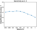
(a) Sensitivity w.r.t. $\lambda$.

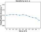
(b) Sensitivity w.r.t. $\alpha$.

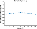
(c) Sensitivity w.r.t. $\gamma$.

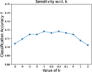
(d) Sensitivity w.r.t. $k$.

Figure 3: Sensitivity of PLCP.

Kernel Extension

The linear classifier in Eq. (5) in the main paper may lack some ability to tackle the complex relationships among the data. Therefore, we extend it to a kernel version. Denote $\phi(\cdot):\mathbb{R}^{q}\rightarrow\mathbb{R}^{h}$ the feature mapping that maps the feature space to some higher dimension space with $h$ dimensions, then we can rewrite Eq. (5) in the main paper as

$$\begin{split}\min_{\hat{\mathbf{W}},\hat{\mathbf{b}}}\quad&\|\mathbf{Z}\|_{F}^{2}+\lambda\|\hat{\mathbf{W}}\|_{F}^{2}\\ {\rm s.t.}\quad&\mathbf{Z}=\mathbf{\Phi}\hat{\mathbf{W}}+\mathbf{1}_{n}\hat{\mathbf{b}}^{\mathsf{T}}-\mathbf{C},\end{split}$$ (15)

where $\mathbf{\Phi}=[\phi(\mathbf{x}_{1}),\phi(\mathbf{x}_{2}),...,\phi(\mathbf{x}_{n})]$. The Lagrangian function of this problem is

$$\begin{split}&\mathcal{L}(\hat{\mathbf{W}},\hat{\mathbf{b}},\mathbf{Z},\mathbf{A})=\|\mathbf{Z}\|_{F}^{2}+\lambda\|\hat{\mathbf{W}}\|_{F}^{2}\\ &-{\rm tr}(\mathbf{A}^{\mathsf{T}}(\mathbf{\Phi}\hat{\mathbf{W}}+\mathbf{1}_{n}\hat{\mathbf{b}}^{\mathsf{T}}-\mathbf{C}-\mathbf{Z})),\end{split}$$ (16)

where $\mathbf{A}=[a_{ij}]_{n\times l}\in\mathbb{R}^{n\times l}$ stores the Lagrange multipliers. Following the KKT conditions:

$$\begin{split}&\frac{\partial\mathcal{L}}{\partial\hat{\mathbf{W}}}=2\lambda\hat{\mathbf{W}}-\mathbf{\Phi}^{\mathsf{T}}\mathbf{A}=0,\frac{\partial\mathcal{L}}{\partial\hat{\mathbf{b}}}=\mathbf{A}^{\mathsf{T}}\mathbf{1}_{n}=0,\\ &\frac{\partial\mathcal{L}}{\partial\mathbf{Z}}=2\mathbf{Z}+\mathbf{A}=0,\frac{\partial\mathcal{L}}{\partial\mathbf{A}}=\mathbf{\Phi}\hat{\mathbf{W}}+\mathbf{1}_{n}\hat{\mathbf{b}}^{\mathsf{T}}-\mathbf{C}-\mathbf{Z}=0.\end{split}$$ (17)

we have the corresponding solution:

$$\begin{split}&\hat{\mathbf{W}}=\frac{\mathbf{\Phi}^{\mathsf{T}}\mathbf{A}}{2\lambda},\mathbf{A}=\left(\frac{1}{2\lambda}\mathbf{K}+\frac{1}{2}\mathbf{I}_{n\times n}\right)^{-1}\left(\mathbf{C}-\mathbf{1}_{n}\hat{\mathbf{b}}^{\mathsf{T}}\right),\\ &\mathbf{s}=\mathbf{1}_{n}^{\mathsf{T}}\left(\frac{1}{2\lambda}\mathbf{K}+\frac{1}{2}\mathbf{I}_{n\times n}\right)^{-1},\hat{\mathbf{b}}^{\mathsf{T}}=\frac{\mathbf{s}\mathbf{C}}{\mathbf{s1}_{n}},\end{split}$$ (18)

where $\mathbf{K}=\mathbf{\Phi}\mathbf{\Phi}^{\mathsf{T}}$ is the kernel matrix with its element $k_{ij}=\phi(\mathbf{x}_{i})^{\mathsf{T}}\phi(\mathbf{x}_{j})=\mathcal{K}(\mathbf{x}_{i},\mathbf{x}_{j})$ based on the kernel function $\mathcal{K}(\cdot,\cdot)$. For PLCP, Gaussian function $\mathcal{K}(\mathbf{x}_{i},\mathbf{x}_{j})={\rm exp}(-\frac{\|\mathbf{x}_{i}-\mathbf{x}_{j}\|_{2}^{2}}{2\sigma^{2}}$) is adopted as the kernel function with $\sigma$ to the average distance of all pairs of training samples. The modeling output is denoted by

$$\hat{\mathbf{M}}=\frac{1}{2\lambda}\mathbf{KA}+\mathbf{1}_{n}\hat{\mathbf{b}}^{\mathsf{T}}.$$ (19)

Deep-learning Extension

Extension to Deep-learning Based Method

PLCP can be also extended to a deep-learning version to further demonstrate its universality and effectiveness. The model of the majority of the deep-learning based methods usually contains a feature encoder followed by a prediction head, which predicts the labeling confidence of each sample. Denote a model in $\mathcal{B}$ with such architecture $g(\cdot)$, specifically, an additional model $\hat{g}(\cdot)$ with the same architecture as $g(\cdot)$ is introduced as the partner classifier, which predicts the non-candidate labeling confidence of each sample. Given an example $\mathbf{x}$ and its candidate label vector $\mathbf{y}$, the non-candidate loss is defined as

$$\mathcal{L}_{com}=-\sum_{i=1}^{l}(1-y_{i})\log(\hat{g}_{i}(\mathbf{x})).$$ (20)

Afterwards, a collaborative loss is designed to link the two models:

$$\mathcal{L}_{col}=\sum_{i=1}^{l}p_{i}\hat{p}_{i}.$$ (21)

Here, $\mathbf{p}=[p_{1},p_{2},...,p_{l}]$ and $\hat{\mathbf{p}}=[\hat{p}_{1},\hat{p}_{2},...,\hat{p}_{l}]$ are two blurred predictions of $g(\mathbf{x})$ and $\hat{g}(\mathbf{x})$ respectively, where

$$\begin{split}\mathbf{p}&=\frac{\phi(e^{k}g(\mathbf{x}))\odot\mathbf{y}}{(\phi(e^{k}g(\mathbf{x}))\odot\mathbf{y})\mathbf{1}_{l}}\\ \hat{\mathbf{p}}&=\mathbf{1}_{l}^{\mathsf{T}}-\frac{\phi(e^{k}(1-\hat{g}(\mathbf{x})))\odot\mathbf{y}}{(\phi(e^{k}(1-\hat{g}(\mathbf{x})))\odot\mathbf{y})\mathbf{1}_{l}}.\end{split}$$ (22)

The overall loss function is:

$$\mathcal{L}=\mathcal{L}_{ori}+\mathcal{L}_{com}+\mu\mathcal{L}_{col},$$ (23)

where $\mathcal{L}_{ori}$ is the original loss function of $\mathcal{B}$ and $\mu$ is a hyper-parameter.

Implementation Details

In PLCP, we set $k=-1$ and $\mu=0.5$. All the hyper-parameters and experimental setups of $\mathcal{B}$ are set based on their original papers.

Details on Real-world Data Sets

The characteristics of the real-world data sets are shown in Tab. 5. Moreover, we present the complete experiments on real-world data sets here.

References

- Chai, Tsang, and Chen (2020) Chai, J.; Tsang, I. W.; and Chen, W. 2020. Large Margin Partial Label Machine. IEEE Trans. Neural Networks Learn. Syst., 31(7): 2594–2608.
- Cour et al. (2009) Cour, T.; Sapp, B.; Jordan, C.; and Taskar, B. 2009. Learning from ambiguously labeled images. In 2009 IEEE Computer Society Conference on Computer Vision and Pattern Recognition (CVPR 2009), 20-25 June 2009, Miami, Florida, USA, 919–926. IEEE Computer Society.
- Cour, Sapp, and Taskar (2011) Cour, T.; Sapp, B.; and Taskar, B. 2011. Learning from Partial Labels. J. Mach. Learn. Res., 12: 1501–1536.
- Fan et al. (2021) Fan, J.; Yu, Y.; Wang, Z.; and Gu, J. 2021. Partial label learning based on disambiguation correction net with graph representation. IEEE Transactions on Circuits and Systems for Video Technology, 32(8): 4953–4967.
- Feng and An (2018) Feng, L.; and An, B. 2018. Leveraging Latent Label Distributions for Partial Label Learning. In Lang, J., ed., Proceedings of the Twenty-Seventh International Joint Conference on Artificial Intelligence, IJCAI 2018, July 13-19, 2018, Stockholm, Sweden, 2107–2113. ijcai.org.
- Feng and An (2019) Feng, L.; and An, B. 2019. Partial Label Learning with Self-Guided Retraining. In The Thirty-Third AAAI Conference on Artificial Intelligence, AAAI 2019, The Thirty-First Innovative Applications of Artificial Intelligence Conference, IAAI 2019, The Ninth AAAI Symposium on Educational Advances in Artificial Intelligence, EAAI 2019, Honolulu, Hawaii, USA, January 27 - February 1, 2019, 3542–3549. AAAI Press.
- Gao and Zhang (2021) Gao, Y.; and Zhang, M.-L. 2021. Discriminative complementary-label learning with weighted loss. In International Conference on Machine Learning, 3587–3597. PMLR.
- Gong, Yuan, and Bao (2022) Gong, X.; Yuan, D.; and Bao, W. 2022. Partial Label Learning via Label Influence Function. In Chaudhuri, K.; Jegelka, S.; Song, L.; Szepesvári, C.; Niu, G.; and Sabato, S., eds., International Conference on Machine Learning, ICML 2022, 17-23 July 2022, Baltimore, Maryland, USA, volume 162 of Proceedings of Machine Learning Research, 7665–7678. PMLR.
- Guillaumin, Verbeek, and Schmid (2010) Guillaumin, M.; Verbeek, J.; and Schmid, C. 2010. Multiple Instance Metric Learning from Automatically Labeled Bags of Faces. In Daniilidis, K.; Maragos, P.; and Paragios, N., eds., Computer Vision - ECCV 2010, 11th European Conference on Computer Vision, Heraklion, Crete, Greece, September 5-11, 2010, Proceedings, Part I, volume 6311 of Lecture Notes in Computer Science, 634–647. Springer.
- Han et al. (2018) Han, B.; Yao, Q.; Yu, X.; Niu, G.; Xu, M.; Hu, W.; Tsang, I. W.; and Sugiyama, M. 2018. Co-teaching: Robust training of deep neural networks with extremely noisy labels. In Bengio, S.; Wallach, H. M.; Larochelle, H.; Grauman, K.; Cesa-Bianchi, N.; and Garnett, R., eds., Advances in Neural Information Processing Systems 31: Annual Conference on Neural Information Processing Systems 2018, NeurIPS 2018, December 3-8, 2018, Montréal, Canada, 8536–8546.
- He et al. (2022) He, S.; Feng, L.; Lv, F.; Li, W.; and Yang, G. 2022. Partial Label Learning with Semantic Label Representations. In Proceedings of the 28th ACM SIGKDD Conference on Knowledge Discovery and Data Mining, 545–553.
- Huiskes and Lew (2008) Huiskes, M. J.; and Lew, M. S. 2008. The MIR flickr retrieval evaluation. In Lew, M. S.; Bimbo, A. D.; and Bakker, E. M., eds., Proceedings of the 1st ACM SIGMM International Conference on Multimedia Information Retrieval, MIR 2008, Vancouver, British Columbia, Canada, October 30-31, 2008, 39–43. ACM.
- Hüllermeier and Beringer (2005) Hüllermeier, E.; and Beringer, J. 2005. Learning from Ambiguously Labeled Examples. In Famili, A. F.; Kok, J. N.; Sánchez, J. M. P.; Siebes, A.; and Feelders, A. J., eds., Advances in Intelligent Data Analysis VI, 6th International Symposium on Intelligent Data Analysis, IDA 2005, Madrid, Spain, September 8-10, 2005, Proceedings, volume 3646 of Lecture Notes in Computer Science, 168–179. Springer.
- Ishida et al. (2017) Ishida, T.; Niu, G.; Hu, W.; and Sugiyama, M. 2017. Learning from Complementary Labels. 5639–5649.
- Ishida et al. (2019) Ishida, T.; Niu, G.; Menon, A.; and Sugiyama, M. 2019. Complementary-label learning for arbitrary losses and models. In International Conference on Machine Learning, 2971–2980. PMLR.
- Jia, Si, and Zhang (2023) Jia, Y.; Si, C.; and Zhang, M.-l. 2023. Complementary Classifier Induced Partial Label Learning. arXiv preprint arXiv:2305.09897.
- Jin and Ghahramani (2002a) Jin, R.; and Ghahramani, Z. 2002a. Learning with multiple labels. Advances in neural information processing systems, 15.
- Jin and Ghahramani (2002b) Jin, R.; and Ghahramani, Z. 2002b. Learning with Multiple Labels. In Becker, S.; Thrun, S.; and Obermayer, K., eds., Advances in Neural Information Processing Systems 15 [Neural Information Processing Systems, NIPS 2002, December 9-14, 2002, Vancouver, British Columbia, Canada], 897–904. MIT Press.
- Katsura and Uchida (2020) Katsura, Y.; and Uchida, M. 2020. Bridging ordinary-label learning and complementary-label learning. In Asian Conference on Machine Learning, 161–176. PMLR.
- Krizhevsky, Hinton et al. (2009) Krizhevsky, A.; Hinton, G.; et al. 2009. Learning multiple layers of features from tiny images.
- Li, Guo, and Zhou (2021) Li, Y.; Guo, L.; and Zhou, Z. 2021. Towards Safe Weakly Supervised Learning. IEEE Trans. Pattern Anal. Mach. Intell., 43(1): 334–346.
- Li and Liang (2019) Li, Y.; and Liang, D. 2019. Safe semi-supervised learning: a brief introduction. Frontiers Comput. Sci., 13(4): 669–676.
- Liu and Dietterich (2012) Liu, L.; and Dietterich, T. G. 2012. A Conditional Multinomial Mixture Model for Superset Label Learning. 557–565.
- Liu and Dietterich (2014) Liu, L.; and Dietterich, T. G. 2014. Learnability of the Superset Label Learning Problem. In Proceedings of the 31th International Conference on Machine Learning, ICML 2014, Beijing, China, 21-26 June 2014, volume 32 of JMLR Workshop and Conference Proceedings, 1629–1637. JMLR.org.
- Lv et al. (2020) Lv, J.; Xu, M.; Feng, L.; Niu, G.; Geng, X.; and Sugiyama, M. 2020. Progressive identification of true labels for partial-label learning. In international conference on machine learning, 6500–6510. PMLR.
- Lyu, Wu, and Feng (2022) Lyu, G.; Wu, Y.; and Feng, S. 2022. Deep graph matching for partial label learning. In Proceedings of the International Joint Conference on Artificial Intelligence, 3306–3312.
- Nguyen and Caruana (2008) Nguyen, N.; and Caruana, R. 2008. Classification with partial labels. In Li, Y.; Liu, B.; and Sarawagi, S., eds., Proceedings of the 14th ACM SIGKDD International Conference on Knowledge Discovery and Data Mining, Las Vegas, Nevada, USA, August 24-27, 2008, 551–559. ACM.
- Panis et al. (2016) Panis, G.; Lanitis, A.; Tsapatsoulis, N.; and Cootes, T. F. 2016. Overview of research on facial ageing using the FG-NET ageing database. IET Biom., 5(2): 37–46.
- Papandreou et al. (2015) Papandreou, G.; Chen, L.; Murphy, K. P.; and Yuille, A. L. 2015. Weakly-and Semi-Supervised Learning of a Deep Convolutional Network for Semantic Image Segmentation. In 2015 IEEE International Conference on Computer Vision, ICCV 2015, Santiago, Chile, December 7-13, 2015, 1742–1750. IEEE Computer Society.
- Qian et al. (2023) Qian, W.; Li, Y.; Ye, Q.; Ding, W.; and Shu, W. 2023. Disambiguation-based partial label feature selection via feature dependency and label consistency. Information Fusion, 94: 152–168.
- Ren et al. (2018) Ren, M.; Zeng, W.; Yang, B.; and Urtasun, R. 2018. Learning to Reweight Examples for Robust Deep Learning. In Dy, J. G.; and Krause, A., eds., Proceedings of the 35th International Conference on Machine Learning, ICML 2018, Stockholmsmässan, Stockholm, Sweden, July 10-15, 2018, volume 80 of Proceedings of Machine Learning Research, 4331–4340. PMLR.
- Wang, Zhang, and Li (2022) Wang, D.; Zhang, M.; and Li, L. 2022. Adaptive Graph Guided Disambiguation for Partial Label Learning. IEEE Trans. Pattern Anal. Mach. Intell., 44(12): 8796–8811.
- Wang et al. (2022) Wang, H.; Xiao, R.; Li, Y.; Feng, L.; Niu, G.; Chen, G.; and Zhao, J. 2022. Pico: Contrastive label disambiguation for partial label learning. arXiv preprint arXiv:2201.08984.
- Wu, Wang, and Zhang (2022) Wu, D.-D.; Wang, D.-B.; and Zhang, M.-L. 2022. Revisiting consistency regularization for deep partial label learning. In International Conference on Machine Learning, 24212–24225. PMLR.
- Xia et al. (2023) Xia, S.; Lv, J.; Xu, N.; Niu, G.; and Geng, X. 2023. Towards Effective Visual Representations for Partial-Label Learning. In Proceedings of the IEEE/CVF Conference on Computer Vision and Pattern Recognition, 15589–15598.
- Xu, Lv, and Geng (2019) Xu, N.; Lv, J.; and Geng, X. 2019. Partial label learning via label enhancement. In Proceedings of the AAAI Conference on artificial intelligence, volume 33, 5557–5564.
- Xu et al. (2021) Xu, N.; Qiao, C.; Geng, X.; and Zhang, M.-L. 2021. Instance-dependent partial label learning. Advances in Neural Information Processing Systems, 34: 27119–27130.
- Yu and Zhang (2017) Yu, F.; and Zhang, M. 2017. Maximum margin partial label learning. volume 106, 573–593.
- Zeng et al. (2013) Zeng, Z.; Xiao, S.; Jia, K.; Chan, T.; Gao, S.; Xu, D.; and Ma, Y. 2013. Learning by Associating Ambiguously Labeled Images. In 2013 IEEE Conference on Computer Vision and Pattern Recognition, Portland, OR, USA, June 23-28, 2013, 708–715. IEEE Computer Society.
- Zhang and Yu (2015) Zhang, M.; and Yu, F. 2015. Solving the Partial Label Learning Problem: An Instance-Based Approach. 4048–4054.
- Zhang, Zhou, and Liu (2016) Zhang, M.; Zhou, B.; and Liu, X. 2016. Partial Label Learning via Feature-Aware Disambiguation. In Krishnapuram, B.; Shah, M.; Smola, A. J.; Aggarwal, C. C.; Shen, D.; and Rastogi, R., eds., Proceedings of the 22nd ACM SIGKDD International Conference on Knowledge Discovery and Data Mining, San Francisco, CA, USA, August 13-17, 2016, 1335–1344. ACM.
- Zhang, Wu, and Bao (2022) Zhang, M.-L.; Wu, J.-H.; and Bao, W.-X. 2022. Disambiguation enabled linear discriminant analysis for partial label dimensionality reduction. ACM Transactions on Knowledge Discovery from Data (TKDD), 16(4): 1–18.
- Zhou (2018) Zhou, Z.-H. 2018. A brief introduction to weakly supervised learning. National science review, 5(1): 44–53.
- Zhu and Goldberg (2009) Zhu, X.; and Goldberg, A. B. 2009. Introduction to Semi-Supervised Learning.