Learning Top-$k$ Subtask Planning Tree based on Discriminative Representation Pre-training for Decision Making

Abstract.

Many complicated real-world tasks can be broken down into smaller, more manageable parts, and planning with prior knowledge extracted from these simplified pieces is crucial for humans to make accurate decisions. However, replicating this process remains a challenge for AI agents and naturally raises two questions: How to extract discriminative knowledge representation from priors? How to develop a rational plan to decompose complex problems? Most existing representation learning methods employing a single encoder structure are fragile and sensitive to complex and diverse dynamics. To address this issue, we introduce a multiple-encoder and individual-predictor regime to learn task-essential representations from sufficient data for simple subtasks. Multiple encoders are able to extract adequate task-relevant dynamics without confusion, and the shared predictor can discriminate task’s characteristics. We also use the attention mechanism to generate a top-k subtask planning tree, which customizes subtask execution plans in guiding complex decisions on unseen tasks. This process enables forward-looking and globality by flexibly adjusting the depth and width of the planning tree. Empirical results on a challenging platform composed of some basic simple tasks and combinatorially rich synthetic tasks consistently outperform some competitive baselines and demonstrate the benefits of our design.

1. Introduction

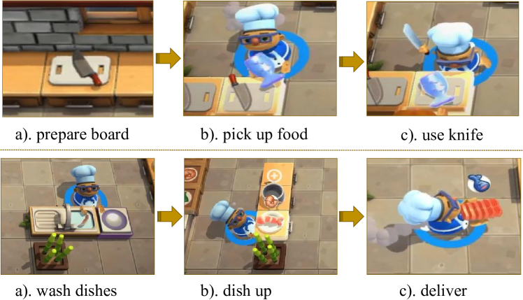
Figure 1. Taking two scenarios in Overcooked AI Carroll et al. (2019) for example, the top denotes cutting food, and the bottom is serving customers. Cutting food should take command of solving a sequence of subtasks: prepare the chopping board, pick up an onion, and use a knife to cut. The execution of serving customers should perform: wash dishes, dish up, and deliver.

Decomposing complex problems into smaller, and more manageable subtasks with some priors and then solving them step by step is one of the critical human abilities. In contrast, reinforcement learning (RL) Schulman et al. (2017); Haarnoja et al. (2018); Konda and Tsitsiklis (1999); Babaeizadeh et al. (2016) agents typically learn from scratch and need to collect a large amount of experience, which is expensive, especially in the real world. An efficient solution is to utilize subtask priors to extract sufficient knowledge representations and transduce them into decision conditions to assist policy learning. Many real-world challenging problems with different task structures can be solved with the subtask-conditioned reinforcement learning (ScRL) regime, such as robot skill learning Kase et al. (2020); Mülling et al. (2013); Cambon et al. (2009); Gao et al. (2019); Wurman et al. (2008), navigation Zhu et al. (2017); Zhu and Zhang (2021); Quan et al. (2020); Gupta et al. (2022), and cooking Carroll et al. (2019); Knott et al. (2021); Sarkar et al. (2022). ScRL endows an agent with the learned knowledge to perform corresponding subtasks, and the subtask execution path should be planned in a rational manner. Ideally, the agent should master some basic competencies to finish some subtasks, and composite the existing subtasks to find an optimal decision path to solve previously unseen and complicated problems. For example, if the final goal is to perform an unseen task like cutting onions, the agent should be able to prepare a chopping board, pick up an onion, and use a knife. For a clear understanding, we visualize two different task structures by recombining subtask sequences, as shown in figure 1.

There are two challenges in ScRL. A fundamental question is how to construct proper knowledge representations about subtasks to transfer to more complicated tasks. The content and structure of knowledge representation are vital to the reasoning of the decision-making, since they refer to functional descriptions of different subtasks to reach the final goal. Another is how to utilize the learned knowledge to assist policy training. Most previous works Netanyahu et al. (2022); Yuan and Lu (2022); Jang et al. (2022); Ryu et al. (2022) mainly focus on zero-shot generalization on unseen tasks of the same scale, instead of recombining prior knowledge to plan more complicated tasks for guiding policy learning.

To address the above issues, our key idea is to construct proper knowledge representations, recombine existing knowledge, and apply it in policy training to improve training efficiency and model performance. We first introduce a learning regime based on multiple-encoder and individual-predictor to extract distinguishable subtask representations with task-essential properties. This module aims to exploit underlying task-specific features and construct proper knowledge representations using contrastive learning and model-based dynamic prediction. Each encoder corresponds to each subtask, which alleviates the disturbing burden of other subtasks on representation extraction to some extent. Next, we propose a construction algorithm for generating a top-$k$ subtask planning tree to customize the subtask execution plan for the agent. Then we use the subtask-conditioned reinforcement learning framework to obtain the decision policy. The top-$k$ subtask planning tree can grow to any width and depth for solving complicated tasks of different scales. Long-term planning for the future can prevent the agent from moving towards local optima as far as possible.

The contributions of this paper can be summarized as follows.

• We introduce a multiple-encoder and individual-predictor learning regime to learn distinguishable subtask representations with task-essential properties.

• We propose to construct a top-$k$ subtask planning tree to customize subtask execution plans for learning with subtask-conditioned reinforcement learning.

• Empirical evaluations on several challenging navigation tasks show that our method can achieve superior performance and obtain meaningful results consistent with intuitive expectations.

2. Related Work

Task representation

One line of research, including HiP-BMDP 
Zhang et al. (2020), MATE Schäfer et al. (2022), MFQI D’Eramo et al. (2020), CARE Sodhani et al. (2021), CARL Benjamins et al. (2021), etc, is designed to achieve fast adaptation by aggregating experience into a latent representation on which policy is conditioned to solve the zero/few-shot generalization in multi-task RL. Another line, such as CORRO Yuan and Lu (2022), MerPO Lin et al. (2021), FOCAL Li et al. (2020), FOCAL++ Li et al. (2021), etc, mainly focuses on learning the task/context embeddings with fully offline meta-RL to mitigate the distribution mismatch of behavior policies in training and testing. Among all the aforementioned approaches, this paper is the most related to the latter. Part of our work is devoted to finding the proper subtask representations using offline datasets to assist online policy learning.

Task planning

Task planning is essentially breaking down the final goals into a sequence of subtasks. Based on the style of planning, we classify the existing approaches into three categories: planning with priors, planning on latent space, and planning with implicit knowledge. First, planning with priors will generate one or more task execution sequences according to the current situation and the subtask function prior, such as Kuffner and LaValle (2000); Liang et al. (2022); Garrett et al. (2021); Okudo and Yamada (2021), but is limited by subtasks divided by human labor. Second, planning on latent space Jurgenson et al. (2020); Pertsch et al. (2020); Zhang et al. (2021); Ao et al. (2021) endows agents with the ability to reason over an imagined long-horizon problem, but it is fundamentally bottlenecked by the accuracy of the learned dynamics model and the horizon of a task. Third, some works like Kaelbling and Lozano-Pérez (2017); Yang et al. (2022, 2020), utilize the modular combination for implicit knowledge injection to reach indirect task guidance and planning, which lack explainability. Our work aims to obtain proper knowledge representation extracted from the subtask itself, and generate a rational and explainable subtask tree including one or more task execution sequences.

Subtask-conditioned RL (ScRL)

ScRL requires the agent to make decisions according to different subtasks, which has been studied in a number of prior works Sohn et al. (2018); Sutton et al. (2022); Mehta et al. (2005); Nasiriany et al. (2019); Chane-Sane et al. (2021); Ghosh et al. (2018); Zhang et al. (2022). However, the existing works mainly solve the short-horizon subtask and rarely focus on the recombination of the learned subtask to solve the complicated long-horizon missions. We propose an explicit subtask representation and scheduling framework to provide long-horizon planning and guidance.

3. Methodology

In this section, we first describe our problem setup. Then we introduce how to learn distinguishable subtask representations as the cornerstone. Next, we propose to construct a top-$k$ subtask planning tree to customize subtask execution plans for the agent. After these, we introduce the policy learning assisted by the tree for decision making.

3.1. Problem Setup

Temporal Subtask-conditioned Markov Decision Process (TSc-MDP)

We consider augmenting a finite-horizon Markov decision process Howard (1960) $(\mathcal{S},\mathcal{A},p,r,{\rho_{0}},\gamma)$ with an extra tuple $(\{{\mathcal{T}^{i}}\}_{i=0}^{n},$ $sp,$ ${\rho_{s}})$ as the temporal subtask-conditioned Markov decision process, where $\mathcal{S}$, $\mathcal{A}$ denote the state space and the action space, respectively. $\{{\mathcal{T}^{i}}\}_{i=0}^{n}$ is the subtask set and $n$ is the number of subtasks. $p(s_{t+1},\mathcal{T}_{t+1}^{i}|s_{t},\mathcal{T}_{t}^{i},a_{t})$ is the dynamics function that gives the distribution of the next state $s_{t+1}$ and next subtask $\mathcal{T}_{t+1}^{i}$ at state $s_{t}$ to execute the subtask $\mathcal{T}_{t}^{i}$ and take action $a_{t}$. $r:\mathcal{S}\times\mathcal{T}\times\mathcal{A}\to\mathbb{R}$ denotes the reward function. $\rho_{0}$ and $\rho_{s}$ denote the initial state distribution and the subtask distribution. $\gamma\in(0,1)$ is the discount factor. $sp$ is the temporal subtask planner that generates subtask sequences at a coarse time scale. Formally, the optimization objective is to find the optimal policy $\pi$ and the subtask planner $sp$ to maximize the expected cumulative return:

$$J(\pi,sp)={\mathbb{E}_{\scriptstyle{a_{t}}\sim\pi(\cdot|{s_{t}})\hfill\atop\mathcal{T}_{t}^{i}\sim\rm{sp}(\cdot|\tau)\hfill}}\left[{\sum\nolimits_{t}{{\gamma^{t}}r({s_{t}},\mathcal{T}_{t}^{i},{a_{t}})}}\right],$$ (1)

where $\tau$ is the history transitions.

3.2. Distinguishable Subtask Representations

Data Collection.

Due to the time-consuming and often ineffective training for complex tasks, directly collecting expert data is intractable. Therefore, we disassemble the complex task into a set of multiple simple tasks, denoted as $\mathcal{T}:\{\mathcal{T}^{1},\mathcal{T}^{2},...,\mathcal{T}^{n}\}$. Simple tasks can easily be trained from scratch to obtain optimal policies. For collecting diverse and relevant data and eliminate the effect of the behaviour policies, we collect 1000 trajectories separately from the optimal, the intermediate trained, and the random policy for each subtask. The collected data format for subtask $\mathcal{T}^{i}$ can be denoted as $\{(s_{t},a_{t},r_{t},s_{t+1})_{t=1}^{L}\}^{i}$, where $L$ is the trajectory length. The data collection statistics are shown in Appendix A.1.

Representation Pre-training.

In reinforcement learning domain, the environmental system is characterized by a transition function and a reward function. Therefore, what we need to do is to use the collected trajectories to mine the essential properties of subtasks and make proper representations from the perspective of the transition and the reward function. To learn accurate and discriminative subtask representations, we introduce a multiple-encoder and individual-predictor learning regime to extract task-essential properties, as shown in Figure 2.

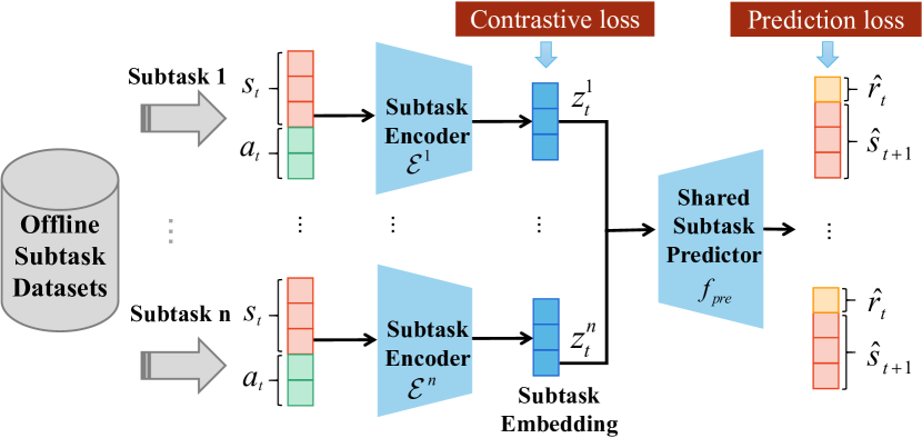
Figure 2. The multiple-encoder and individual-predictor learning regime. Each subtask encoder $\mathcal{E}^{i}$ is used to encode the state-action pair $(s_{t},a_{t})^{i}\in\mathcal{T}^{i}$ and output the compact subtask representation $z_{t}^{i}$. The shared subtask predictor is used to predict the reward $r_{t}$ and the next state $s_{t+1}$. The contrastive and prediction losses are designed to learn the many to one framework.

There are two design principles: i) Each subtask has its own different responsibilities and skills, so multiple encoders can boost the diversity among them. On the other hand, multiple subtask encoders, which each corresponds to one subtask, can effectively avoid mapping two state-action pairs from different subtasks with various reward and transition distributions to similar abstractions. ii) Figuring out the essential properties of transition and reward function is the key to obtaining accurate and generalizable subtask representations, so we design an auxiliary prediction task to simulate the reward and transition distributions. The shared subtask predictor is used to predict the reward and the next state so as to implicitly learn the world model for a better understanding of the accurate essential properties of the subtasks.

Supposed that we have $n$ subtasks, we initialize $n$ subtask encoders parameterized by $\{\theta^{i}\}_{i=1}^{n}$, respectively. First, we sample a minibatch of $b$ transitions $\{\tau^{i}_{j}=(s_{j},a_{j},r_{j},s_{j+1})^{i}\}_{j=1}^{b}$ from some subtask $\mathcal{T}^{i}$, and feed the state-action pairs $\{(s_{j},a_{j})^{i}\}_{j=1}^{b}$ to the subtask encoder $\mathcal{E}^{i}:\mathcal{S}\times\mathcal{A}\mapsto\mathcal{Z}$. Then the latent variables $z^{i}\in\mathcal{Z}$ for subtask $\mathcal{T}^{i}$ are obtained, denoted as $z^{i}=\mathcal{E}^{i}((s,a)^{i})$.

After obtaining the latent variables of different subtasks, for better distinguishment, a contrastive loss is applied, where samples from the other subtasks act as negative pairs. First, we define $x=(s,a)$, $x^{+}=(s^{+},a^{+})$, and $x^{-}=(s^{-},a^{-})$ as the current, the positive, and the negative state-action pairs, respectively. Given the current subtask id $i$, we have the latent variables, denoted as $q={\mathcal{E}^{i}}(s,a)$, $k^{+}={\mathcal{E}^{i}}(s^{+},a^{+})$, $k^{-}={\mathcal{E}^{j}}(s^{-},a^{-})$, and $j$ is the other subtask ids except $i$. Therefore, the contrastive learning objective Oord et al. (2018) for the multiple subtask encoders is:

$${\mathcal{L}_{c}^{i}}=-\log\frac{{\exp({q}\cdot{k^{+}})}}{{\exp({q}\cdot{k^{+}})+\sum_{k^{-}}{\exp({q}\cdot{k^{-}})}}}.$$ (2)

The full set $\mathbb{X}=\{x_{0},x_{1},...\}$ can be explicitly partitioned as $P(\mathbb{X})=\{\{x^{+}\},\{x^{-}\}\}$, where $x^{+}$ is from the current subtask, $x^{-}$ comes from the other $n-1$ subtasks, and $\{x^{-}\}$=$\mathbb{X}\backslash\{x^{+}\}$. Benefiting from this, the multiple transition encoders should extract the essential variance of transition and reward functions across different tasks and mine the shared and compact features of the same subtasks.

As for the shared subtask predictor $f_{pre}$, we use the mean squared error (MSE) loss to calculate the mean overseen data of the squared differences between true and prediction as follows.

$${\mathcal{L}_{p}}={\lambda_{r}}||\hat{r}-r||_{2}^{2}+{\lambda_{s}}||\hat{s}^{\prime}-s^{\prime}||_{2}^{2}\ ,$$ (3)

where $\hat{r},\hat{s}^{\prime}=f_{pre}(z)$ is the prediction of the immediate reward $r$ and the next state $s^{\prime}$. $\lambda_{r}$ and $\lambda_{s}$ are positive scalars that tune the relative weights between the loss terms.

With contrastive learning for pushing inter-tasks and pulling intra-task and dynamics prediction for mining nature properties, the total loss is summarized as follows.

$$\min\sum\limits_{subtask\ i}{\sum\limits_{\scriptstyle{\tau^{i}}\sim{\mathcal{T}^{i}}\atop\scriptstyle{\tau^{\{n\}\backslash i}}\sim{\mathcal{T}^{\{n\}\backslash i}}}{(\mathcal{L}_{c}^{i}+{\mathcal{L}_{p}})}},$$ (4)

where $\tau=(s,a,r,s^{\prime})$, and $\{n\}$ are the collected transitions and the total subtask set.

After finishing the first step toward compact representations for subtasks, the subtask tree can be generated.

3.3. Top-$k$ Subtask Planning Tree Generation

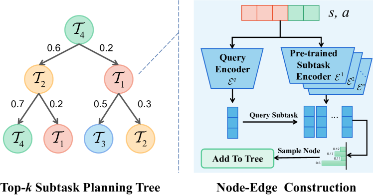
Figure 3. The left part is a top-$2$ subtask treewhich is generated by the process of the right part.

In real human society, effective decision-making always relies on good judgment of the current state, and future prediction and imagination. Enlightened by this ability of humanity, we should generate a top-$k$ subtask tree to assist the policy training. Due to the long horizon and sparse feedback of complicated tasks, we adjust the subtask tree generation during rollout instead of generating a specified tree for one task. As shown in figure 2, we generate a relatively short-horizon subtask tree with some inference of dynamics in a coarse-to-fine manner and a new subtask tree will regenerate once the current tree has been executed to a leaf node. Next, we describe the generation process in detail as follows.

First, we provide the detailed construction procedure of the subtask tree in a top-down manner. Here, we have a query encoder $\mathcal{E}^{q}$ and the $n$ pre-trained encoder $\{\mathcal{E}^{i}\}^{n}_{i=1}$ corresponding to each subtask defined in section 3.2.

Node-edge construction process.

At the current timestep $t$, due to the limitation that we can only touch the last action $a_{t-1}$, we compute the query vector $v^{q}$ as the anchor to retrieve the most similar subtask.

$${v^{q}}={{{{\mathcal{E}}}}^{q}}({s_{t-1}},{a_{t-1}}).$$ (5)

Next, the subtask embeddings from the pre-trained encoder can be obtained as follows.

$$\{{v^{i}}\}_{i=1}^{n}=\{{{\mathcal{E}}^{i}}({s_{t-1}},{a_{t-1}})\}_{i=1}^{n}.$$ (6)

We utilize the attention mechanism Bahdanau et al. (2015) to compute the correlation score between the query vector $v^{q}$ and the pre-trained subtask embeddings $\{{v^{i}}\}_{i=1}^{n}$. Then the normalized coefficient $\alpha_{q,i}$ is defined:

$${\alpha_{q,i}}=\frac{{\exp({\beta_{q,i}})}}{{\sum\nolimits_{j}{\exp({\beta_{q,j}})}}},\ where\ {\beta_{q,i}}={v^{q}}{W^{T}_{\phi}}W_{\varphi}{v^{i}},$$ (7)

where $W_{\phi},W_{\varphi}$ are learnable parameters and $\beta_{q,i}$ is the attention score. Here, we can model the correlation between query vector $v^{q}$ and an arbitrary number of subtasks, which allows us to easily increase the number of subtasks in our tree generation process. Then the categorical distribution can be modeled using the weights from which the variable $C$ can be sampled:

$$C\sim{\mathcal{P}_{\beta}}=Categorical\left({\frac{{\exp({\beta_{q,i}})}}{{\sum\nolimits_{j\in\mathcal{N}}{\exp({\beta_{q,j}})}}},i\in\mathcal{N}=\{1,...,n\}}\right).$$ (8)

Then, given the hyperparameter $k<n$, we can sample the top-$k$ subtask ids without replacement from the categorical distribution which means sampling the first element, then renormalizing the remaining probabilities to sample the next element, etcetera. Let $C_{1}^{*},...,C_{k}^{*}$ be an (ordered) sample without replacement from the Categorical $\mathcal{P}_{\beta}$, then the joint probability can be formulated as follows.

$$P(C_{1}^{*}=c_{1}^{*},...,C_{k}^{*}=c_{k}^{*})=\prod\limits_{i=1}^{k}{\frac{{\exp({\beta_{q,c_{i}^{*}}})}}{{\sum\nolimits_{\iota\in\mathcal{N}_{i}^{*}}{\exp({\beta_{q,\iota}})}}}},$$ (9)

where $c_{1}^{*},...,c_{k}^{*}=argtop$-$k({\mathcal{P}_{\beta}})$is the sampled top-$k$ realization of variables $C_{1}^{*},...,C_{k}^{*}$, and $\mathcal{N}_{i}^{*}=\mathcal{N}\backslash\{c_{1}^{*},...,c_{i-1}^{*}\}$ is the domain (without replacement) for the $i$-th sampled element.

Then, we use the sampled top-$k$ subtask ids as the $k$ nodes at a certain layer in the subtask tree (Please note that we set $k=1$ while generating the root node). Moreover, given the hyperparameter $N$, we can obtain the tree of depth $N$ by repeating the above process based on the planning transition (described in the next paragraph), and the original correlation weight ${\alpha_{q,i}}$ is set as connections (edges) between layer and layer. For a clear understanding, we summarize the overall construction procedure shown in figure 4.

Planning for future: $m$-step predictor

While expanding the subtask tree, we should make planning for the $m$-step prediction of the future. We design a $m$-step predictor denoted as $p_{m}(\hat{s}_{t+m}|\hat{s}_{t},\hat{a}_{t})$ that is used to derive the next $m^{th}$ step’s state. The action $\hat{a}_{t+m}$ is output by the policy network $\pi$ (defined in Equation (16)) using the current subtask representation. The $N$-times rollout starting with $s_{t-1}$ can be written as:

$$\left\{{({s_{t-1}},{a_{t-1}}),({{\hat{s}}_{t+m-1}},{{\hat{a}}_{t+m-1}}),...,({{\hat{s}}_{t+N\cdot m-1}},{{\hat{a}}_{t+N\cdot m-1}})}\right\}.$$

Then we can use this imagined rollout to expand the subtask tree to a greater depth. That is, as each layer of depth increases, the planning will perform $m$-step imagination forward.

Figure 4. The basic top-$k$ subtask tree construction process.

Optimization for tree generation

The optimization includes two parts: an $m$-step predictor $p_{m}$ and an attention module. The former $p_{m}$ can be trained by minimizing the mean squared error function $\mathcal{L}_{m}$ defined as follows. Sampled some state-action pairs from replay buffer $\mathcal{D}$, we have:

$$\mathcal{L}_{m}={\mathbb{E}_{\scriptstyle({s_{t}},{a_{t}},{s_{t+m}})\sim\mathcal{D}\hfill\atop\scriptstyle{{\hat{s}}_{t+m}}={p_{m}}({s_{t}},{a_{t}})\hfill}}\left[{||{{\hat{s}}_{t+m}},{s_{t+m}}||_{2}^{2}}\right].$$ (10)

The attention module parameterized by $\omega=\{\phi,\varphi\}$ can be optimized in a Monte-Carlo policy gradient manner Williams (1992). First, we define the intra-subtask cumulative reward $R_{t}=\sum\nolimits_{j=0}^{\tilde{T}-1}{{\gamma^{j}}{r_{t+j}}}$ during the interval $\tilde{T}$ of the subtask execution process as follows. By decomposing the cumulative rewards into a Bellman Expectation equation in a recursive manner, we acquire:

$$G({s_{t}},{\mathcal{T}_{t}})=\mathbb{E}\left[{R_{t+1}+{\gamma}G({s_{t+\tilde{T}}},{\mathcal{T}_{t+\tilde{T}}})|{s_{t}},{\mathcal{T}_{t}}}\right],$$ (11)

where ${s_{t}}$ and ${\mathcal{T}_{t}}$ is the current state and the executed subtask, $\gamma$ is the discounted factor, and ${\mathcal{T}_{t+\tilde{T}}}$ is the next subtask.

Then, by applying the mini-batch technique to the off-policy training, the gradient updating can be approximately estimated as:

$$\omega\leftarrow\omega+\alpha\nabla\log{\mathcal{P}_{\beta}}({\mathcal{T}_{t}}|{s_{t-1},a_{t-1}})\cdot{G(s_{t},\mathcal{T}_{t})},$$ (12)

where $t$ denotes the timestep when a subtask execution begins and $\alpha$ is the learning rate.

3.4. Tree-auxiliary Policy

Given a generated top-$k$ subtask tree, we can obtain a tree-auxiliary policy as follows. Generally, agents should have the foresight to judge the current situation, give a rational plan, and then use the plan to guide policy learning. Therefore, the first step is to generate a plan based on the top-$k$ subtask tree.

Subtask execution plan generation

Here, we design a discounted upper confidence bound (d-UCB) method for the path finding. For each subtask $\mathcal{T}^{i}$, we record its selection count $c_{\mathcal{T}^{i}}$ and the average cumulative rewards $r_{\mathcal{T}^{i}}$ while the subtask terminates. The UCB value for the $\mathcal{T}^{i}$ in the planning tree is computed as:

$$v_{\mathcal{T}^{i}}=r_{\mathcal{T}^{i}}+0.5\cdot\sqrt{\frac{2\ln c_{{\mathcal{T}^{i}}}^{pa}}{c_{\mathcal{T}^{i}}}},$$ (13)

where $c_{{\mathcal{T}^{i}}}^{pa}$ is the selection count of the parent node of $\mathcal{T}_{i}$.

Then, we give a definition of the discounted path length via the evaluation of d-UCB. We adopt the greedy policy to pick the path (subtask execution plan) with the maximum discounted length. The detailed intuition description is shown in Appendix A.2.

Definition 0.

Sample a path from root to leaf in the tree, the length of the discounted path can be defined as follows.

$${{\hat{d}}}(root\to leaf)=\sum\nolimits_{l}{{\kappa^{l}}{e^{l,l+1}}\cdot v_{\mathcal{T}^{i}}},$$

where $e^{l,l+1}$ is a sampled edge between $l^{th}$ layer and $(l+1)^{th}$ layer, the value of the edge is the probability of subtask transition, $\kappa=0.8$ is the discounted factor, and $v_{\mathcal{T}^{i}}$ is the UCB value of the sampled node in the $(l+1)^{th}$ layer.

Subtask termination condition

Subtask execution should be terminated when the current situation changes, and we give a measurement about when to terminate the current subtask. we first calculate the cosine similarity of the current query vector $\mathcal{E}^{q}(s_{t},a_{t})$ and the corresponding subtask embedding $\mathcal{E}^{\mathcal{T}_{id}}(s_{t},a_{t})$ and the similarity function is defined as follows.

$$Sim({{{{\mathcal{E}}}}^{q}}({s_{t}},{a_{t}}),{{{{\mathcal{E}}}}^{{{{{\mathcal{T}}}}_{id}}}}({s_{t}},{a_{t}}))=\frac{{\left({{{({{{{\mathcal{E}}}}^{q}}({s_{t}},{a_{t}}))}^{T}}{{{{\mathcal{E}}}}^{{{{{\mathcal{T}}}}_{id}}}}({s_{t}},{a_{t}})}\right)}}{{\left({||{{{{\mathcal{E}}}}^{q}}({s_{t}},{a_{t}})||\cdot||{{{{\mathcal{E}}}}^{{{{{\mathcal{T}}}}_{id}}}}({s_{t}},{a_{t}})||}\right)}}.$$ (14)

For every timestep, the agent will compare the similarity score of the current timestep and the last timestep. If the similarity score decreases more than a threshold $\Delta=0.5$, the subtask will terminate and turn to the next one until the path ends.

Subtask-guided decision making

In our implementation, the policy will consider the current state and the subtask embedding and give a comprehensive decision, formulated as follows.

$$a_{t}\sim\pi(\cdot|s_{t},\mathcal{E}^{\mathcal{T}_{id}}(s_{t-1},a_{t-1})).$$ (15)

As for the policy optimization, we adopt the PPO-style Schulman et al. (2017) training regime and the objective function is defined as follows.

$${\mathcal{L}_{\pi}}=\left[{\min\left({{i_{t}}\cdot{A_{t}},clip({i_{t}},1-\varepsilon,1+\varepsilon){A_{t}}}\right)}\right],$$ (16)

where $i_{t}=\frac{{\pi({a_{t}}|{s_{t}},{{{{\mathcal{E}}}}^{{{{{\mathcal{T}}}}_{id}}}}(s_{t-1},a_{t-1}))}}{{{\pi_{old}}({a_{t}}|{s_{t}},{{{{\mathcal{E}}}}^{{{{{\mathcal{T}}}}_{id}}}}(s_{t-1},a_{t-1}))}}$ is the importance ratio, and $A_{t}$ is is an estimator of the advantage function at timestep $t$.

All in all, the overall optimization flow including subtask representation pre-training, top-k subtask generation and tree-auxiliary policy is summarized in Algorithm 1.

Ensure subtask representation policy $\rho=\{\{\mathcal{E}^{i}\}_{i=1}^{n},f_{pre}\}$, tree building policy $\mathcal{E}^{q}$, and tree-axuliary policy $\pi$;

// Subtask Representation Pre-training

Collect diverse subtask datasets $\{\mathcal{T}^{1},...,\mathcal{T}^{k}\}$;

for each iteration do

       Sample a subtask $\mathcal{T}^{i}$ and transitions $\{\tau^{i}_{t}\}_{t=1}^{b}$, $\{\tau^{i,+}_{t}\}_{t=1}^{b}$;

       $\{z^{i}_{t}\}_{t=1}^{l}=\{\mathcal{E}^{i}(s_{t}^{i},a_{t}^{i})\}_{t=1}^{l}$ ;

       $\{z^{i,+}_{t}\}_{t=1}^{l}=\{\mathcal{E}^{i}(s_{t}^{i,+},a_{t}^{i,+})\}_{t=1}^{l}$ ;

       Sample other subtasks $\mathcal{T}\backslash\mathcal{T}^{i}$ and transitions $\{\tau^{i,-}_{t}\}_{t=1}^{b}$;

       $\{z^{i,-}_{t}\}_{t=1}^{l}=\{\mathcal{E}^{-}(s_{t}^{i,-},a_{t}^{i,-})\}_{t=1}^{l}$ ;

       Predict reward $r$ and next state $s^{\prime}$;

       Update $\rho$ to minimize Eq. (4);

      

end for

// Tree Generation and Tree-auxiliary Policy

for each episode do

       Initial state-action pair $s\_a_{cur}=(s_{0},a_{0})$;

       BUILD_TREE($s\_a_{cur},\mathcal{E}^{q},\{\mathcal{E}^{i}\}_{i=1}^{n}$) ; // Fig. 4

       Use d-UCB in Sec. 3.4 to find a plan $\zeta$;

       for each timestep $t$ do

             if  $\zeta$ is None  then

                   Regenerate the tree and the plan;

                  

             end if

            while $\zeta$ is not None do

                   $\mathcal{T}_{id}=\zeta[0]$;

                   // execute current subtask Select action $a_{t}=\pi(\cdot|s_{t},\mathcal{E}^{\mathcal{T}_{id}}(s\_a_{cur}))$;

                   Receive reward $r$ and next state $s^{\prime}$ ;

                   if  $Sim({{{{\mathcal{E}}}}^{q}}({s_{t}},{a_{t}}),{{{{\mathcal{E}}}}^{{{{{\mathcal{T}}}}_{id}}}}({s_{t}},{a_{t}}))<0.5$  then

                         remove $\mathcal{T}_{id}$ from $\zeta$; // execute next subtask

                        

                   end if

                  

             end while

            

       end for

      Update $\pi$ with Eq. (16);

       Update $\mathcal{E}^{q}$ with Eq. (10) and Eq. (12);

      

end for

Algorithm 1 Overall Procedure

4. Experiments

In this section, we seek to empirically evaluate our method to verify the effectiveness of our solution. We design the experiments to 1) verify the effectiveness of the multiple-encoder and individual-predictor learning regime; 2) test the performance of our top-$k$ subtask tree on the most complicated scenarios in the 2D navigation task BabyAI Chevalier-Boisvert et al. (2019); 3) conduct some ablation studies in our settings.

(a) Open

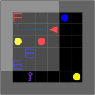
(b) Go to

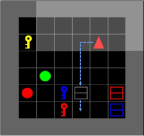
(c) Put next

(d) Pick up

Figure 5. The schematics of four basic subtasks. The dashed lines denote the path to reach the goal. The agent represented by the red triangle is partially observable to the grid and the light-grey shaded area represents its field of view. The missions are described as : (a). Open the red door; (b). Go to the red box; (c). Put the grey box next to the red key. (d). Pick up the green ball.

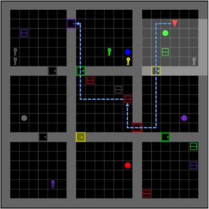
Figure 6. The illustration for one of the BossLevel scenario. The mission is: ”pick up a red box and go to the purple door”.

4.1. Experimental Setting

We choose BabyAI as our experimental platform, which incorporates some basic subtasks and some composite complex tasks. For each scenario, there are different small subtasks, such as opening doors of different colors. The agent should focus on the skill of opening doors, rather than the color itself. Moreover, the BabyAI platform provides by default a $7\times 7\times 3$ symbolic observation $o_{t}$ (a partial and local egocentric view of the state of the environment) and a variable length instruction $c$ as inputs at each time step $t$.

Basic Subtask

BabyAI contains four basic subtasks that may appear in more complicated scenarios, including Open, Goto, PutNext, and Pickup, as shown in figure 5. (a) Open : Open the door with a certain color and a certain position, e.g. ”open the green door on your left”. The color set and position set are defined as : $COLOR=\{red,\ green,$ $blue,\ purple,$ $yellow,\ grey\}$ and $POS=\{on\ your\ left,\ on\ your\ right,$ $\ in\ front\ of\ you,\ behind$ $\ you\}$. (b) Goto : Go to an object that the subtask instructs, e.g. ”go to red ball” means going to any of the red balls in the maze. The object set is defined as: $OBJ=\{door,\ box,\ ball,\ key\}$. (c) PutNext : Put objects next to other objects, e.g. ”put the blue key next to the green ball”. (d) PickupLoc : Pick up some objects, e.g.“pick up a box”.

Complicated Task

The BabyAI platform includes some tasks that require three or more subtasks compositions to solve, which are called complicated tasks. What we want to do is to solve these tasks through our tree-based policy to reach higher performance and faster convergence. Take the ”BossLevel” scenario for example, the agent should follow one of the instructions like ”pick up the grey box behind you, then go to the grey key and open a door”, which contains three subtasks and is shown as figure 6. More detailed descriptions are shown in Appendix A.3.

Baselines

In this paper, we select the state-of-the-art (SOTA) algorithm PPO Schulman et al. (2017) and SAC Haarnoja et al. (2018), the tree-based planning algorithm SGT Jurgenson et al. (2020), and the context-based RL method CORRO Yuan and Lu (2022) as baselines to verify the effectiveness of our proposed method. PPO is a popular deep reinforcement learning algorithm for solving discrete and continuous control problems, which is an on-policy algorithm. SAC is an off-policy actor-critic deep RL algorithm based on the maximum entropy reinforcement learning framework. SGT adopts the divide-and-conquer style that recursively predicts intermediate sub-goals between the start state and goal. It can be interpreted as a binary tree that is most similar to our settings. CORRO is based on the framework of context-based meta-RL, which adopts a transition encoder to extract the latent context as a policy condition.

Parameter Settings

Additionally, we provide the description of all the neural networks used in our framework and more detailed experimental hyperparameter settings in Appendix A.4 and Appendix A.5, respectively.

4.2. Results on Subtask Representaion

Here report the experimental visualization results on the settings described in Section 3.2 to verify the effectiveness of our distinguishable subtask representations, shown as Figure 7.

(a) 2 subtasks

(b) 3 subtasks

(c) 4 subtasks

(d) 2 subtasks

(e) 3 subtasks

(f) 4 subtasks

Figure 7. The t-SNE visualization of subtask embeddings. (a-c): The results are generated by our multiple encoders and one predictor learning regime on 2, 3, and 4 subtasks, respectively. (d-f): Substitute our multiple encoder modules with one shared encoder and regenerate the visualization.

Firstly, we train our multiple encoders and individual predictor with collected diverse subtask datasets on 2, 3, and 4 subtasks, respectively. Then we substitute the multiple encoder modules with one shared encoder and train it. Figure 7 visualizes the t-SNE Van der Maaten and Hinton (2008) 2D projection of the latent subtask embeddings for these two models. The results show that our regime is capable of clearly illustrating separate clusters of embeddings for different tasks no matter how many subtasks or encoders we use. However, only one shared encoder can not learn the boundaries and distinguishment clearly and we speculate that mixed representation training for multiple different subtasks would interfere with the stabilization of the representation module.

Moreover, due to the powerful capacity of contrastive learning and model-based dynamic prediction, our model can exhibit strong representational discrimination and contain enough dynamics knowledge, which will be verified empirically as follows.

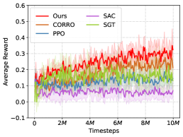
(a) GoToSeq

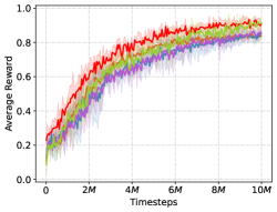
(b) GoToSeqS5R2

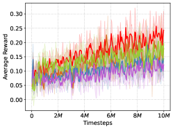
(c) SynthSeq

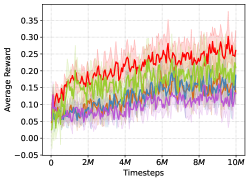
(d) BossLevel

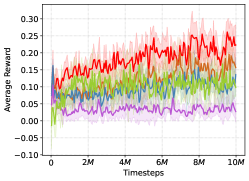
(e) BossLevelNoUnlock

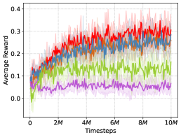
(f) MiniBossLevel

Figure 8. The training curve comparisons on six complicated tasks, averaged over 10 independent running seeds.

4.3. Results on Training Curves

To evaluate our method in complicated and dynamic environments, we conduct various experiments on multiple difficulty levels of BabyAI, elaborated in Appendix A.3. These levels require multiple competencies to solve them. For example, GotoSeq only requires navigating a room or maze, recognizing the location, and understanding the sequence subtasks while BossLevel requires mastering all competencies including navigating, opening, picking up, putting next, and so on.

Here, we report the average episode reward by training steps for each level, averaged over 10 independent running seeds to plot the reward curve with standard deviation. In GoToSeqS5R2 which is the relatively simplest level in the six, all the test rewards keep increasing as the training steps increase and almost reach the best finally. In other complicated tasks, our algorithm consistently obtains higher rewards than all the baselines in the different levels of BabyAI shown in Figure 8, while the popular SOTA like PPO and SAC almost fail. This indicates that our method is capable of macro-planning and robust enough to handle the complicated tasks by decomposing the overall process into a sequence of execution subtasks.

Although we only trained 10M timesteps due to the limitation of computing resources, our method has a higher starting point than the baseline model, and it has been rising. However, the gain of the baselines at the same timestep is not obvious in most cases. This significant improvement is mainly due to two aspects. On the one hand, the adequate knowledge representation facilitates the inference capacity of our model and gives a high-level starting point for warming up the training. On the other hand, the learned subtask planning strategy can make rational decisions while confronting various complicated situations.

4.4. Results on Execution Performance

To further test the execution performance of all methods, we freeze the trained policies and execute for 100 episodes, and report the mean and standard deviations in Table 1. Our algorithm can consistently and stably outperform all the competitive baselines by a large margin, which demonstrates the benefits of our framework.

Table 1. Execution performance on various complicated tasks. We report the average reward with standard deviations of 100 testing episodes with best values in bold.

	Ours	CORRO	PPO	SAC	SGT
GoToSeq	0.30$\pm$0.07	0.23$\pm$ 0.06	0.14$\pm$ 0.04	0.05$\pm$ 0.04	0.15$\pm$ 0.08
GoToSeqS5R2	0.91$\pm$ 0.02	0.84$\pm$ 0.02	0.84$\pm$ 0.03	0.85$\pm$ 0.02	0.91$\pm$ 0.04
SynthSeq	0.22$\pm$ 0.05	0.16$\pm$ 0.05	0.12$\pm$ 0.05	0.12$\pm$ 0.04	0.18$\pm$ 0.05
BossLevel	0.26$\pm$ 0.05	0.15$\pm$ 0.04	0.14$\pm$ 0.05	0.12$\pm$ 0.04	0.19$\pm$ 0.06
BossLevelNoUnlock	0.24$\pm$ 0.04	0.17$\pm$ 0.04	0.10$\pm$ 0.05	0.04$\pm$ 0.03	0.11$\pm$ 0.05
MiniBossLevel	0.29$\pm$ 0.06	0.26$\pm$ 0.05	0.25$\pm$ 0.05	0.06$\pm$ 0.03	0.14$\pm$ 0.06

4.5. Results on Various Tree Width

After the verification of the training and execution performance of our technique, we perform in-depth ablation studies regarding the width of the planning tree shown in Figure 9. Here, we freeze the tree depth as $3$, same as the main experiments. Additional experimental results about other scenarios can be found in Appendix A.6.

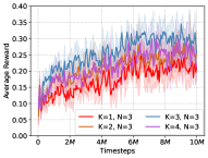
(a) BossLevel

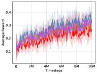
(b) GotoSeq

Figure 9. The ablations on various tree width.

The horizontal axis represents the training steps, and the vertical axis is the average episode reward with a standard deviation, averaged across 10 independent running seeds. According to our intuition, the wider the tree is, the more diverse the subtask distribution is. However, according to the experimental results, we find that the gain is not the largest when the width of the tree is the largest. We speculate that as the width of the tree is larger, more information can be selected, but the pertinence of problem-solving is not strong, which is easy to cause confusion. Therefore, it is critical to choose an appropriate tree width and it is our future direction to conduct the adaptive selection.

4.6. Results on Various Tree Depth

As shown in Figure 10, we further provide in-depth ablation studies to understand the behavior of our planning tree depending on various tree depths. Here, we freeze the tree width as $2$, the same as the main experiments. Then we provide more ablation studies in Appendix A.7. The depth represents the capacity for predicting the future of our planning tree. As shown in Figure 10, the results show that when the depth $N=2$ or $N=3$, our model wins the comparable performance also. However, the curves about $N=4$ shows the degraded performance than others. We analyze that the prediction error about the future at every step keeps accumulating, so it may make the model go in a bad direction although the foresight ability can help the model make a global decision.

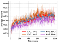
(a) BossLevel

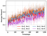
(b) GotoSeq

Figure 10. The ablations on various tree depth.

4.7. Results on Subtask Execution Statistics

As shown in Figure 11, we visualize the subtask proportion on six complicated tasks after testing 1000 episodes respectively. It is surprisingly consistent with the pre-defined task missions. It basically corresponds to predefined tasks, which intuitively justifies the rationality of our approach. For example, GoToSeq and GoToSeqS5R2 only require the competency of executing some sequences about“Go To”, our model focuses on this subtask during the execution in most cases. There exists some error that other tasks will be selected occasionally, and we speculate that it is because of the inaccuracy of forward prediction during expanding the depth of the tree. Our model executes subtasks at roughly the same frequency when dealing with the other four tasks which require comprehensive competencies.

Figure 11. The bars represent the mean proportion of each subtask executed by our trained model over 1000 episodes.

5. Conclusion

In this paper, we have considered the difficulties of task planning to solve complicated problems, and propose a two-stage planning framework. The multiple-encoder and individual-predictor regime can extract discriminative subtask representations with dynamic knowledge from priors. The top-k subtask planning tree, which customizes subtask execution plans to guide decisions, is important in complicated tasks. Generalizing our model to unseen and complicated tasks demonstrates significant performance and exhibits greater potential to deploy it to real-life complicated tasks. More ablation studies also demonstrate the capacity of our planning tree.

For future works, it would be interesting to automatically learn more explainable subtasks and make influential and global planning as a reference to human decisions in real-life applications.

Appendix A Appendix

A.1. Detailed Statistics about the Collected Data

The data collection statistics are shown as Table 2, of which 1/3 is collected from the converged PPO policy, 1/3 is collected from the intermediate trained checkpoint of PPO, and the last 1/3 is from the random policy.

Subtask	#Total Episodes	#Total Transitions
PickupLoc	3000	210375
PutNext	3000	559201
Goto	3000	218191
Open	3000	149349

Table 2. The data collection statistics

A.2. Detailed Description about the Intuition for d-UCB

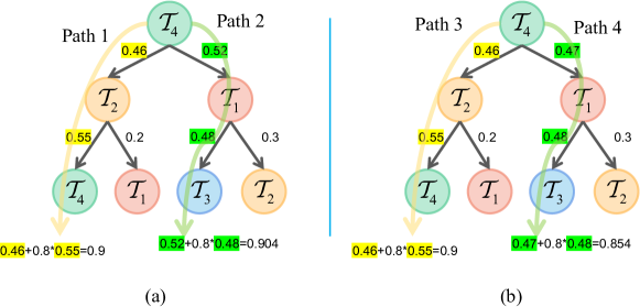
Figure 12. Two instance trees are visualized to verify the effect of d-UCB described in Section 3.4. To ignore the effect of UCB value, we set the value of all nodes as $1$.

Here, we provide another two methods. One is called max selection (MS), which means that MS will pick the path in that the cumulative probability is maximum. Next, we will compare it with our d-UCB method. Another is called greedy selection (GS), which means that GS will pick the current maximum probability layer by layer. Next, we will compare it with our d-UCB method.

As shown in Figure 12(a), MS will select path $1$, which obviously places a greater weight on the future with greater uncertainty. However, our d-UCB will choose path $2$, which tends to maximize the immediate benefit by discounting the future uncertain score, which is consistent with our intuition.

Moreover, as shown in Fig. 12(b), not like MS tending to pick the edge with the highest probability, our d-UCB will choose path $3$. Our d-UCB also considers the optimal subtask to perform in the future when the nearest paths exhibit similar transition probabilities.

A.3. Detailed Description about Complicated Tasks

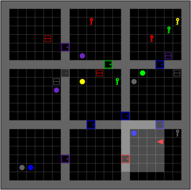
(a) ‘BabyAI-BossLevel-v0’

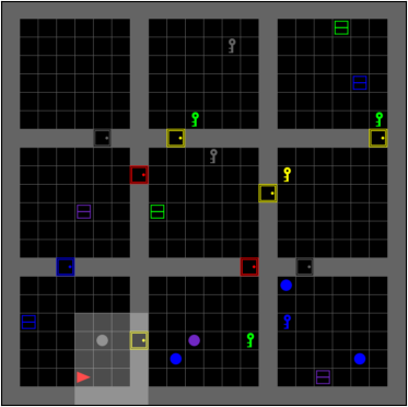
(b) ‘BabyAI-BossLevelNoUnlock-v0’

(c) ‘BabyAI-MiniBossLevel-v0’

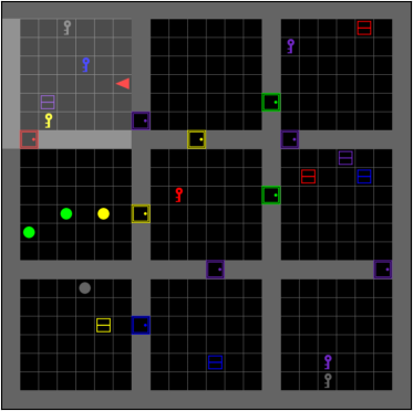
(d) ‘BabyAI-GoToSeq-v0’

(e) ‘BabyAI-GoToSeqS5R2-v0’

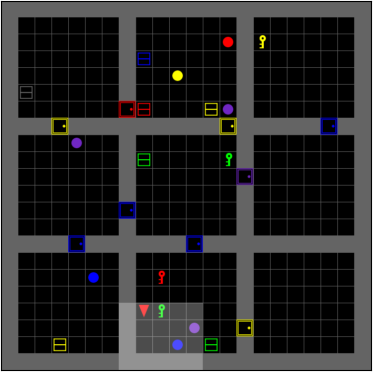
(f) ‘BabyAI-SynthSeq-v0’

Figure 13. The diagrams for six complicated tasks in BabyAI.

BossLevel

The level requires the agent to implement any union of instructions produced according to Baby Language grammar, it involves the content of all other levels. For example, “open a door and pick up the green key after you go to a ball and put a red box next to the red ball” is a command of the level. This level requires all the competencies including navigating, unblocking, unlocking, opening, going to, picking up, putting next, and so on.

BossLevelNoUnlock

The doors of all rooms are unlocked which the agent can go through without unlocking by a corresponding key. For example, the command “open a purple door, then go to the yellow box and put a yellow key next to a box” doesn’t need the agent to get a key before opening a door. This level requires all the competencies like BossLevel except unlocking.

MiniBossLevel

The level is a mini-environment of BossLevel with fewer rooms and a smaller size. This level requires all the competencies like BossLevel except unlocking.

GoToSeq

The agent needs to complete a series of go-to-object commands in sequence. For example, the command ”go to a grey key and go to a purple key, then go to the green key” only includes go-to instructions. GotoSeq only requires navigating a room or maze, recognizing the location, and understanding the sequence subtasks.

GoToSeqS5R2

The missions are just like GoToSeq, which requires the only competency of “go to”. Here, S5 and R2 refer to the size and the rows of room, respectively.

SynthSeq

The commands, which combine different kinds of instructions, must be executed in order.For example, ”open the purple door and pick up the blue ball, then put the grey box next to a ball”. This level requires the competencies like GotoSeq except inferring whether to unlock or not.

A.4. Network Architecture

There is a summary of all the neural networks used in our framework about the network structure, layers, and activation functions.

	Network Structure	Layers	Hidden Size	Activation Functions
Subtask Encoder	MLP	6	[256, 256, 128, 128, 32]	ReLu
Shared Subtask Predictor	MLP	3	[64, 128]	ReLu
Query Encoder	MLP	4	[32, 16, 8]	ReLu
Tree Node Generation	CausalSelfAttention	1	-	Softmax
Feature Extractor	CNN+FiLMedBlock	-	-	ReLu
Policy Actor	MLP	2	64	Tanh
Policy Critic	MLP	2	64	Tanh

Table 3. The Summary for Network Architecture

Please note that ’-’ denote that we refer readers to check the open source repository about FiLMedBlock and CausalSelfAttention, see https://github.com/caffeinism/FiLM-pytorch and https://github.com/sachiel321/Efficient-Spatio-Temporal-Transformer, respectively.

A.5. Parameter Settings

There are our hyper-parameter settings for the training of distinguishable subtask representation and the tree-based policy, shown in Table A.5 and Table A.5, respectively.

Description	Value
lr	$3*10^{-4}$
contrastive batch size	$64$
negative pairs number	$16$
task embedding size	$5$
$\lambda_{r}$	$0.9$
$\lambda_{s}$	$1.0$
encoder hidden size	$[256,256,128,128,32]$
decoder hidden size	$[64,128]$

Table 4. Task Representation Hyper-paramters

Description	Value
optimizer	Adam
$\alpha$	$10^{-4}$
$\beta_{1}$	$0.9$
$\beta_{2}$	$0.999$
$\varepsilon$	$10^{-5}$
seed	$[0,10)$
number of process	$64$
total frames	$10M$
lr	$10^{-4}$
batch size	$1280$
eval interval	$1$
eval episodes	$500$
image embedding	$128$
memory of LSTM	$128$
query hidden size	$[32,16,8]$
number of head	$1$
discounted factor of UCB	$0.9$
$m$-step predictor	$5$

Table 5. Tree-based Policy Hyper-paramters

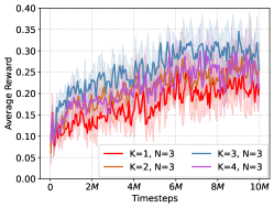
(a) BossLevel

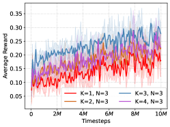
(b) BossLevelNoUnlock

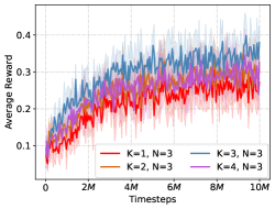
(c) MiniBossLevel

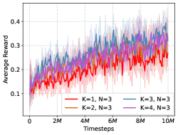
(d) GoToSeq

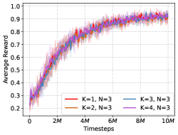
(e) GoToSeqS5R2

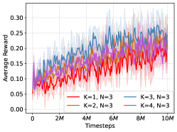
(f) SynthSeq

Figure 14. The ablation study of tree width for other four complicated tasks in BabyAI.

A.6. Additional Experimental Results on Tree Width

As shown in Figure 14, the other four experiments basically presented results consistent with the analysis in the main text. Among them, the experimental environment of GoToSeqSR2 is relatively simpler, and the performance of our model basically reaches the optimal trend, so the ablation study of tree width does not seem to work. We believe that our model is capable of handling complex tasks and is not very discriminative for simple tasks. In addition, for MiniBossLevel, the experiment with a tree width of $2$ achieves the best performance. It indicates that our model can already show a good performance improvement in a slightly simpler environment with a tree width of $2$.

A.7. Additional Experimental Results on Tree Depth

As shown in Figure 15, we plot the training curves of the other four complicated tasks freezing the width as $2$. Combining the experiments in the main text, these results all show a common phenomenon: the larger the value of $N$, the worse the performance of our model. This cumulative effect of errors shows that the accuracy of our tree-building prediction model needs to be improved, and it is also a defect of our model. We will focus on how to improve the forward prediction ability of the model in future work. In addition, changing the depth of the tree in the scene GoToSeqS5R2 still cannot reflect the difference of the model. This shows that our model can achieve excellent performance even if our tree prediction module is not very accurate. On the one hand, this success may depend on the strong fault tolerance of our pre-trained representation model, and the generated representations can correctly guide model learning; on the other hand, it may depend on the design of our subtask termination function, which can stop the subtask in time when the task mismatch is found.

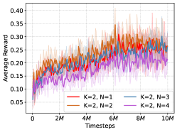
(a) BossLevel

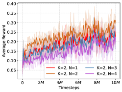
(b) BossLevelNoUnlock

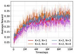
(c) MiniBossLevel

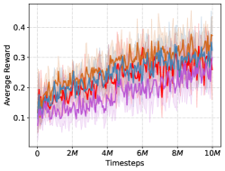
(d) GoToSeq

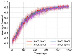
(e) GoToSeqS5R2

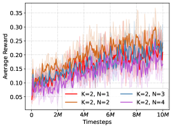
(f) SynthSeq

Figure 15. The ablation study of tree depth for other four complicated tasks in BabyAI.

References

- (1)
- Ao et al. (2021) Shuang Ao, Tianyi Zhou, Guodong Long, Qinghua Lu, Liming Zhu, and Jing Jiang. 2021. CO-PILOT: COllaborative Planning and reInforcement Learning On sub-Task curriculum. Advances in Neural Information Processing Systems (2021).
- Babaeizadeh et al. (2016) Mohammad Babaeizadeh, Iuri Frosio, Stephen Tyree, Jason Clemons, and Jan Kautz. 2016. Reinforcement learning through asynchronous advantage actor-critic on a gpu. arXiv preprint arXiv:1611.06256 (2016).
- Bahdanau et al. (2015) Dzmitry Bahdanau, Kyung Hyun Cho, and Yoshua Bengio. 2015. Neural machine translation by jointly learning to align and translate. International Conference on Learning Representations (2015).
- Benjamins et al. (2021) Carolin Benjamins, Theresa Eimer, Frederik Schubert, André Biedenkapp, Bodo Rosenhahn, Frank Hutter, and Marius Lindauer. 2021. Carl: A benchmark for contextual and adaptive reinforcement learning. arXiv preprint arXiv:2110.02102 (2021).
- Cambon et al. (2009) Stephane Cambon, Rachid Alami, and Fabien Gravot. 2009. A hybrid approach to intricate motion, manipulation and task planning. The International Journal of Robotics Research 28, 1 (2009), 104–126.
- Carroll et al. (2019) Micah Carroll, Rohin Shah, Mark K Ho, Tom Griffiths, Sanjit Seshia, Pieter Abbeel, and Anca Dragan. 2019. On the utility of learning about humans for human-ai coordination. Advances in neural information processing systems (2019).
- Chane-Sane et al. (2021) Elliot Chane-Sane, Cordelia Schmid, and Ivan Laptev. 2021. Goal-conditioned reinforcement learning with imagined subgoals. International Conference on Machine Learning (2021).
- Chevalier-Boisvert et al. (2019) Maxime Chevalier-Boisvert, Dzmitry Bahdanau, Salem Lahlou, Lucas Willems, Chitwan Saharia, Thien Huu Nguyen, and Yoshua Bengio. 2019. BabyAI: First Steps Towards Grounded Language Learning With a Human In the Loop. International Conference on Learning Representations (2019).
- D’Eramo et al. (2020) Carlo D’Eramo, Davide Tateo, Andrea Bonarini, Marcello Restelli, Jan Peters, et al. 2020. Sharing knowledge in multi-task deep reinforcement learning. International Conference on Learning Representations (2020).
- Gao et al. (2019) Xiaofeng Gao, Ran Gong, Tianmin Shu, Xu Xie, Shu Wang, and Song-Chun Zhu. 2019. VRKitchen: An interactive 3D environment for learning real life cooking tasks. (2019).
- Garrett et al. (2021) Caelan Reed Garrett, Rohan Chitnis, Rachel Holladay, Beomjoon Kim, Tom Silver, Leslie Pack Kaelbling, and Tomás Lozano-Pérez. 2021. Integrated task and motion planning. Annual review of control, robotics, and autonomous systems (2021).
- Ghosh et al. (2018) Dibya Ghosh, Abhishek Gupta, and Sergey Levine. 2018. Learning actionable representations with goal-conditioned policies. arXiv preprint arXiv:1811.07819 (2018).
- Gupta et al. (2022) Himanshu Gupta, Bradley Hayes, and Zachary Sunberg. 2022. Intention-Aware Navigation in Crowds with Extended-Space POMDP Planning. International Conference on Autonomous Agents and Multiagent Systems (2022).
- Haarnoja et al. (2018) Tuomas Haarnoja, Aurick Zhou, Kristian Hartikainen, George Tucker, Sehoon Ha, Jie Tan, Vikash Kumar, Henry Zhu, Abhishek Gupta, Pieter Abbeel, et al. 2018. Soft actor-critic algorithms and applications. arXiv preprint arXiv:1812.05905 (2018).
- Howard (1960) Ronald A Howard. 1960. Dynamic programming and markov processes. (1960).
- Jang et al. (2022) Eric Jang, Alex Irpan, Mohi Khansari, Daniel Kappler, Frederik Ebert, Corey Lynch, Sergey Levine, and Chelsea Finn. 2022. Bc-z: Zero-shot task generalization with robotic imitation learning. Conference on Robot Learning (2022), 991–1002.
- Jurgenson et al. (2020) Tom Jurgenson, Or Avner, Edward Groshev, and Aviv Tamar. 2020. Sub-Goal Trees a Framework for Goal-Based Reinforcement Learning. International Conference on Machine Learning (2020).
- Kaelbling and Lozano-Pérez (2017) Leslie Pack Kaelbling and Tomás Lozano-Pérez. 2017. Learning composable models of parameterized skills. International Conference on Robotics and Automation (2017).
- Kase et al. (2020) Kei Kase, Chris Paxton, Hammad Mazhar, Tetsuya Ogata, and Dieter Fox. 2020. Transferable task execution from pixels through deep planning domain learning. International Conference on Robotics and Automation (2020).
- Knott et al. (2021) Paul Knott, Micah Carroll, Sam Devlin, Kamil Ciosek, Katja Hofmann, Anca D Dragan, and Rohin Shah. 2021. Evaluating the robustness of collaborative agents. arXiv preprint arXiv:2101.05507 (2021).
- Konda and Tsitsiklis (1999) Vijay Konda and John Tsitsiklis. 1999. Actor-critic algorithms. Advances in neural information processing systems (1999).
- Kuffner and LaValle (2000) James J Kuffner and Steven M LaValle. 2000. RRT-connect: An efficient approach to single-query path planning. International Conference on Robotics and Automation (2000).
- Li et al. (2021) Lanqing Li, Yuanhao Huang, Mingzhe Chen, Siteng Luo, Dijun Luo, and Junzhou Huang. 2021. Provably Improved Context-Based Offline Meta-RL with Attention and Contrastive Learning. arXiv preprint arXiv:2102.10774 (2021).
- Li et al. (2020) Lanqing Li, Rui Yang, and Dijun Luo. 2020. Focal: Efficient fully-offline meta-reinforcement learning via distance metric learning and behavior regularization. arXiv preprint arXiv:2010.01112 (2020).
- Liang et al. (2022) Jacky Liang, Mohit Sharma, Alex LaGrassa, Shivam Vats, Saumya Saxena, and Oliver Kroemer. 2022. Search-based task planning with learned skill effect models for lifelong robotic manipulation. International Conference on Robotics and Automation (2022).
- Lin et al. (2021) Sen Lin, Jialin Wan, Tengyu Xu, Yingbin Liang, and Junshan Zhang. 2021. Model-Based Offline Meta-Reinforcement Learning with Regularization. International Conference on Learning Representations (2021).
- Mehta et al. (2005) Neville Mehta, Prasad Tadepalli, and A Fern. 2005. Multi-agent shared hierarchy reinforcement learning. ICML Workshop on Rich Representations for Reinforcement Learning (2005), 45.
- Mülling et al. (2013) Katharina Mülling, Jens Kober, Oliver Kroemer, and Jan Peters. 2013. Learning to select and generalize striking movements in robot table tennis. The International Journal of Robotics Research 32, 3 (2013), 263–279.
- Nasiriany et al. (2019) Soroush Nasiriany, Vitchyr Pong, Steven Lin, and Sergey Levine. 2019. Planning with goal-conditioned policies. Advances in Neural Information Processing Systems (2019).
- Netanyahu et al. (2022) Aviv Netanyahu, Tianmin Shu, Joshua Tenenbaum, and Pulkit Agrawal. 2022. Discovering Generalizable Spatial Goal Representations via Graph-based Active Reward Learning. International Conference on Machine Learning (2022).
- Okudo and Yamada (2021) Takato Okudo and Seiji Yamada. 2021. Online Learning of Shaping Reward with Subgoal Knowledge. In International Conference on Autonomous Agents and MultiAgent Systems.
- Oord et al. (2018) Aaron van den Oord, Yazhe Li, and Oriol Vinyals. 2018. Representation learning with contrastive predictive coding. arXiv preprint arXiv:1807.03748 (2018).
- Pertsch et al. (2020) Karl Pertsch, Oleh Rybkin, Frederik Ebert, Shenghao Zhou, and et al. 2020. Long-horizon visual planning with goal-conditioned hierarchical predictors. Neural Information Processing Systems (2020).
- Quan et al. (2020) Hao Quan, Yansheng Li, and Yi Zhang. 2020. A novel mobile robot navigation method based on deep reinforcement learning. International Journal of Advanced Robotic Systems 17, 3 (2020), 1729881420921672.
- Ryu et al. (2022) Heechang Ryu, Hayong Shin, and Jinkyoo Park. 2022. REMAX: Relational Representation for Multi-Agent Exploration. International Conference on Autonomous Agents and Multiagent Systems (2022).
- Sarkar et al. (2022) Bidipta Sarkar, Aditi Talati, Andy Shih, and Dorsa Sadigh. 2022. PantheonRL: A MARL Library for Dynamic Training Interactions. AAAI Conference on Artificial Intelligence (2022).
- Schäfer et al. (2022) Lukas Schäfer, Filippos Christianos, Amos Storkey, and Stefano V Albrecht. 2022. Learning task embeddings for teamwork adaptation in multi-agent reinforcement learning. arXiv preprint arXiv:2207.02249 (2022).
- Schulman et al. (2017) John Schulman, Filip Wolski, Prafulla Dhariwal, Alec Radford, and Oleg Klimov. 2017. Proximal policy optimization algorithms. arXiv preprint arXiv:1707.06347 (2017).
- Sodhani et al. (2021) Shagun Sodhani, Amy Zhang, and Joelle Pineau. 2021. Multi-task reinforcement learning with context-based representations. International Conference on Machine Learning (2021).
- Sohn et al. (2018) Sungryull Sohn, Junhyuk Oh, and Honglak Lee. 2018. Hierarchical reinforcement learning for zero-shot generalization with subtask dependencies. Advances in Neural Information Processing Systems (2018).
- Sutton et al. (2022) Richard S Sutton, Marlos C Machado, G Zacharias Holland, David Szepesvari Finbarr Timbers, Brian Tanner, and Adam White. 2022. Reward-Respecting Subtasks for Model-Based Reinforcement Learning. arXiv preprint arXiv:2202.03466 (2022).
- Van der Maaten and Hinton (2008) Laurens Van der Maaten and Geoffrey Hinton. 2008. Visualizing data using t-SNE. Journal of machine learning research 9, 11 (2008).
- Williams (1992) Ronald J Williams. 1992. Simple statistical gradient-following algorithms for connectionist reinforcement learning. Machine learning 8, 3 (1992), 229–256.
- Wurman et al. (2008) Peter R Wurman, Raffaello D’Andrea, and Mick Mountz. 2008. Coordinating hundreds of cooperative, autonomous vehicles in warehouses. AI magazine 29, 1 (2008), 9–9.
- Yang et al. (2022) Mingyu Yang, Jian Zhao, Xunhan Hu, Wengang Zhou, and Houqiang Li. 2022. LDSA: Learning Dynamic Subtask Assignment in Cooperative Multi-Agent Reinforcement Learning. arXiv preprint arXiv:2205.02561 (2022).
- Yang et al. (2020) Ruihan Yang, Huazhe Xu, Yi Wu, and Xiaolong Wang. 2020. Multi-task reinforcement learning with soft modularization. Advances in Neural Information Processing Systems (2020).
- Yuan and Lu (2022) Haoqi Yuan and Zongqing Lu. 2022. Robust Task Representations for Offline Meta-Reinforcement Learning via Contrastive Learning. International Conference on Machine Learning (2022).
- Zhang et al. (2020) Amy Zhang, Shagun Sodhani, Khimya Khetarpal, and Joelle Pineau. 2020. Learning Robust State Abstractions for Hidden-Parameter Block MDPs. International Conference on Learning Representations (2020).
- Zhang et al. (2022) Han Zhang, Jingkai Chen, Jiaoyang Li, Brian C Williams, and Sven Koenig. 2022. Multi-Agent Path Finding for Precedence-Constrained Goal Sequences. International Conference on Autonomous Agents and Multiagent Systems (2022).
- Zhang et al. (2021) Lunjun Zhang, Ge Yang, and Bradly C Stadie. 2021. World model as a graph: Learning latent landmarks for planning. International Conference on Machine Learning (2021).
- Zhu and Zhang (2021) Kai Zhu and Tao Zhang. 2021. Deep reinforcement learning based mobile robot navigation: A review. Tsinghua Science and Technology 26, 5 (2021), 674–691.
- Zhu et al. (2017) Yuke Zhu, Roozbeh Mottaghi, Eric Kolve, Joseph J Lim, Abhinav Gupta, Li Fei-Fei, and Ali Farhadi. 2017. Target-driven visual navigation in indoor scenes using deep reinforcement learning. International Conference on Robotics and Automation (2017).