Testing Self-Reducible Samplers

Abstract

Samplers are the backbone of the implementations of any randomised algorithm. Unfortunately, obtaining an efficient algorithm to test the correctness of samplers is very hard to find. Recently, in a series of works, testers like $\mathsf{Barbarik}$, $\mathsf{Teq}$, $\mathsf{Flash}$ for testing of some particular kinds of samplers, like CNF-samplers and Horn-samplers, were obtained. But their techniques have a significant limitation because one can not expect to use their methods to test for other samplers, such as perfect matching samplers or samplers for sampling linear extensions in posets. In this paper, we present a new testing algorithm that works for such samplers and can estimate the distance of a new sampler from a known sampler (say, uniform sampler).

Testing the identity of distributions is the heart of testing the correctness of samplers. This paper’s main technical contribution is developing a new distance estimation algorithm for distributions over high-dimensional cubes using the recently proposed sub-cube conditioning sampling model. Given subcube conditioning access to an unknown distribution $P$, and a known distribution $Q$ defined over $\{0,1\}^{n}$, our algorithm $\mathsf{CubeProbeEst}$ estimates the variation distance between $P$ and $Q$ within additive error $\zeta$ using $\mathcal{O}\left({n^{2}}/{\zeta^{4}}\right)$ subcube conditional samples from $P$. Following the testing-via-learning paradigm, we also get a tester which distinguishes between the cases when $P$ and $Q$ are $\varepsilon$-close or $\eta$-far in variation distance with probability at least $0.99$ using $\mathcal{O}({n^{2}}/{(\eta-\varepsilon)^{4}})$ subcube conditional samples.

The estimation algorithm in the sub-cube conditioning sampling model helps us to design the first tester for self-reducible samplers. The correctness of the testers is formally proved. On the other hand, we implement our algorithm to create $\mathsf{CubeProbeEst}$ and use it to test the quality of three samplers for sampling linear extensions in posets.

Introduction

Sampling algorithms play a pivotal role in enhancing the efficiency and accuracy of data analysis and decision-making across diverse domains (Chandra and Iyengar 1992; Yuan et al. 2004; Naveh et al. 2006; Mironov and Zhang 2006; Soos, Nohl, and Castelluccia 2009; Morawiecki and Srebrny 2013; Ashur, De Witte, and Liu 2017). With the exponential surge in data volume, these algorithms provide the means to derive meaningful insights from massive datasets without the burden of processing the complete information. Additionally, they aid in pinpointing and mitigating biases inherent in data, ensuring the attainment of more precise and equitable conclusions. From enabling statistical inferences to propelling advancements in machine learning, safeguarding privacy, and facilitating real-time decision-making, sampling algorithms stand as a cornerstone in extracting information from the vast data landscape of our modern world.

However, many advanced sampling algorithms are often prohibitively slow (hash-based techniques of (Chakraborty, Meel, and Vardi 2013; Ermon et al. 2013; Chakraborty et al. 2014; Meel et al. 2016) and MCMC-based methods of (Andrieu et al. 2003; Brooks et al. 2011; Jerrum 1998)) or lack comprehensive verification ((Ermon, Gomes, and Selman 2012), (Dutra et al. 2018), (Golia et al. 2021)). Many popular methods like “statistical tests” rely on heuristics without guarantees of their efficacy. Utilizing unverified sampling algorithms can lead to significant pitfalls, including compromised conclusion accuracy, potential privacy, and security vulnerabilities. Moreover, the absence of verification hampers transparency and reproducibility, underscoring the critical need for rigorous validation through testing, comparison, and consideration of statistical properties. Consequently, a central challenge in this field revolves around designing tools to certify sampling quality and verify correctness, which necessitates overcoming the intricate task of validating probabilistic programs and ensuring their distributions adhere to desired properties.

A notable breakthrough in addressing this verification challenge was achieved by (Chakraborty and Meel 2019), who introduced the statistical testing framework known as “$\mathsf{Barbarik}$”. This method proved instrumental in testing the correctness of uniform CNF (Conjunctive Normal Form) samplers by drawing samples from conditional distributions. $\mathsf{Barbarik}$ demonstrated three key properties: accepting an almost correct sampler with high probability, rejecting a far-from-correct sampler with high probability, and rejecting a “well-behaved” but far-from-correct sampler with high probability. There have been a series of follow-up works (Meel, Pote, and Chakraborty 2020; Pote and Meel 2021, 2022; Banerjee et al. 2023). However, in this framework, conditioning is achieved using a gadget that does not quite generalize to applications beyond CNF sampling. For instance, for linear-extension sampling (Huber 2014), where the goal is to sample a linear ordering agreeing with a given poset, the test requires that the post-conditioning residual input be a supergraph of the original input, with the property that it has exactly two user-specified linear-extensions. This requirement is hard to fulfill in general. On the other hand, a generic tester that would work for any sampler implementation without any additional constraints and simultaneously be sample efficient is too good to be true (Paninski 2008). From a practical perspective, the question is: Can we design an algorithmic framework for testers that would work for most deployed samplers and still have practical sample complexity?

We answer the question positively. We propose algorithms that offer a generic approach to estimating the distance between a known and an unknown sampler, assuming both follow the ubiquitous self-reducible sampling strategy. Our techniques follow a constrained sampling approach, extending its applicability to wide range of samplers without mandating such specific structural conditions. A key foundational contribution of this paper includes leveraging the subcube conditional sampling techniques (Bhattacharyya and Chakraborty 2018) and devising a method to estimate the distance between samplers – a challenge often more intricate than simple correctness testing.

Organization of our paper We first present the preliminaries followed by a description of our results and their relevance. We then give a detailed description of our main algorithms $\mathsf{CubeProbeEst}$ and $\mathsf{CubeProbeTester}$. The detailed theoretical analysis is presented in the supplementary material. We only present a high-level technical overview. Finally, we present our experimental results and conclude.

Preliminaries

In this paper, we are dealing with discrete probability distributions whose sample space is an $n$-dimensional Boolean hypercube, $\{0,1\}^{n}$. For a distribution $\mathcal{D}$ over a universe $\Omega$, and for any $x\in\Omega$, we denote by $\mathcal{D}(x)$ the probability mass of the point $x$ in $\mathcal{D}$. $[n]$ denotes the set $\{1,\ldots,n\}$. For concise expressions and readability, we use the asymptotic complexity notion of $\widetilde{\mathcal{O}}$, where we hide polylogarithmic dependencies of the parameters.

Samplers, Estimators, and Testers

A sampler $\mathcal{I}:\mathsf{Domain}\to\mathsf{Range}$ is a randomized algorithm which, given an input $x\in\mathsf{Domain}$, outputs an element in $\mathsf{Range}$. For a sampler $\mathcal{I}$, $\mathcal{D}^{\mathcal{I},\psi}$ denotes the probability distribution of the output of $\mathcal{I}$ when the input is $\psi\in\mathsf{Domain}$. In other words,

$$\forall x\in\mathsf{Range},\ \mathcal{D}^{\mathcal{I},\psi}(x)=\Pr[\mathcal{I}(\psi)=x],$$

where the probability is over the internal random coins of $\mathcal{I}$.

We define a sampler $\mathcal{I}_{\mathcal{W}}$ to be a known sampler if, for any input $\psi\in\mathsf{Domain}$, we know its probability distribution $\mathcal{D}^{\mathcal{I}_{\mathcal{W}},\psi}$ explicitly. We note that the input $\psi$ depends on the application. For example, in the perfect-matching and linear-extension samplers, $\psi$ is a graph, whereas, for the CNF sampler, $\psi$ is a CNF formula.

Definition 1 (Total variation distance).

Let $\mathcal{I}_{\mathcal{W}}$ and $\mathcal{I}_{\mathcal{G}}$ be two samplers. For an input $\psi\in\mathsf{Domain}$, the variation distance between $\mathcal{I}_{\mathcal{G}}$ and $\mathcal{I}_{\mathcal{W}}$ is defined as:

$$\mathsf{d^{\psi}_{TV}}(\mathcal{I}_{\mathcal{G}},\mathcal{I}_{\mathcal{W}})=\max_{A\subseteq\mathsf{Range}}\{\mathcal{D}^{\mathcal{I}_{\mathcal{G}},\psi}(A)-\mathcal{D}^{\mathcal{I}_{\mathcal{W}},\psi}(A)\}.$$

Definition 2 ($(\zeta,\delta$)-approx $\mathsf{d_{TV}}$ estimator).

A $(\zeta,\delta$)-approx $\mathsf{d_{TV}}$ estimator is a randomized approximation algorithm that given two sampler $\mathcal{I}_{\mathcal{G}}$ and $\mathcal{I}_{\mathcal{W}}$, an input $\psi$, tolerance parameter $\zeta\in(0,1/3]$ and a confidence parameter $\delta\in(0,1)$, with probability $(1-\delta)$ returns an estimation $\widehat{\mathsf{dist}^{\psi}}$ of $\mathsf{d^{\psi}_{TV}}(\mathcal{I}_{\mathcal{G}},\mathcal{I}_{\mathcal{W}})$ such that:

$$\mathsf{d^{\psi}_{TV}}(\mathcal{I}_{\mathcal{G}},\mathcal{I}_{\mathcal{W}})-\zeta\leq\widehat{\mathsf{dist}^{\psi}}\leq\mathsf{d^{\psi}_{TV}}(\mathcal{I}_{\mathcal{G}},\mathcal{I}_{\mathcal{W}})+\zeta$$

Definition 3 ($\varepsilon$-closeness and $\eta$-farness).

Consider any sampler $\mathcal{I}_{\mathcal{G}}$. $\mathcal{I}_{\mathcal{G}}$ is said to be $\varepsilon$-close to another sampler $\mathcal{I}_{\mathcal{W}}$ on input $\psi$, if $\mathsf{d^{\psi}_{TV}}\left(\mathcal{I}_{\mathcal{G}},\mathcal{I}_{\mathcal{W}}\right)\leq\varepsilon$ holds. On the other hand, $\mathcal{I}_{\mathcal{G}}$ is said to be $\eta$-far from $\mathcal{I}_{\mathcal{W}}$ with respect to some input $\psi$ if $\mathsf{d^{\psi}_{TV}}\left(\mathcal{I}_{\mathcal{G}},\mathcal{I}_{\mathcal{W}}\right)\geq\eta$ holds.

Definition 4 ($(\varepsilon,\eta,\delta)$-identity tester)).

An $(\varepsilon,\eta,\delta)$-identity tester takes as input an unknown sampler $\mathcal{I}_{\mathcal{G}}$, a known sampler $\mathcal{I}_{\mathcal{W}}$, an input $\psi$ to the samplers, a tolerance parameter $\varepsilon\in(0,1/3)$, an intolerance parameter $\eta\in(0,1]$ with $\eta>\varepsilon$, a confidence parameter $\delta\in(0,1)$, and with probability at least $(1-\delta)$: (1) outputs ACCEPT if $\mathcal{I}_{\mathcal{G}}$ is $\varepsilon$-close to $\mathcal{I}_{\mathcal{W}}$ on input $\psi$, (2) outputs REJECT if $\mathcal{I}_{\mathcal{G}}$ is $\eta$-far from $\mathcal{I}_{\mathcal{W}}$ on input $\psi$.

For practical purposes, $\delta$ can be $0.99$ or any close-to-one constant. From now onwards, we shall consider the input domain and output range of a sampler to be a Boolean hypercube, that is, $\mathsf{Domain}=\{0,1\}^{m}$ and $\mathsf{Range}=\{0,1\}^{n}$ for some integers $m$ and $n$. Therefore the universe of probability distributions of samplers is $n$-dimensional binary strings.

Self-reducible sampler.

A self-reducible sampler $\mathcal{I}:\{0,1\}^{m}\to\{0,1\}^{n}$ generates a sample $x$ by first sampling a bit and then sampling the rest of the substring. Formally, we can define a self-reducible sampler as follows:

Definition 5 (Self-reducible sampler).

A sampler $\mathcal{I}:\{0,1\}^{m}\to\{0,1\}^{n}$ is said to be a self-reducible sampler if, for any input $\psi\in\{0,1\}^{m}$, there exists $\widehat{\psi}\in\{0,1\}^{m}$ for which the following is true:

$$\mathcal{D}^{\mathcal{I},\psi}(x_{1}x_{2}...x_{n})|_{x_{1}=b_{1},...,x_{i}=b_{i}}=\mathcal{D}^{\mathcal{I},\widehat{\psi}}(b_{1}...b_{i}x_{i+1}...x_{n})$$

where $b_{i}\in\{0,1\}$ for all $i$.

The concept of self-reducibility has been influential in the field of sampling since the work of (Jerrum, Valiant, and Vazirani 1986), which showed the computational complexity equivalence of approximate sampling and counting for problems in #P. Intuitively, self-reducibility is the idea that one can construct the solution to a given problem from the solutions of subproblems of the same problem. Self-reducibility is a critical requirement for simulating subcube conditioning. Also, it does not hamper the model’s generality too much. As observed in (Khuller and Vazirani 1991; Große, Rothe, and Wechsung 2006; Talvitie, Vuoksenmaa, and Koivisto 2020), all except a few known problems are self-reducible.

Subcube Conditioning over Boolean hypercubes

Let $P$ be a probability distribution over $\{0,1\}^{n}$. Sampling using subcube conditioning accepts $A_{1},A_{2},\ldots,A_{n}\subseteq\{0,1\}$, constructs $S=A_{1}\times A_{2}\times\ldots\times A_{n}$ as the condition set, and returns a vector $x=(x_{1},x_{2},\ldots,x_{n})$, such that $x_{i}\in A_{i}$, with probability $P(x)/(\sum_{w\in S}P(w))$. If $P(S)$ = 0, we assume the sampling process would return an element from $S$ uniformly at random. A sampler that follows this technique is called a subcube conditioning sampler.

Linear-Extension of a Poset

We applied our prototype implementation on verifying linear-extension samplers of a poset. Let us first start with the definition of a poset.

Definition 6 (Partially ordered set (Poset)).

Let $S$ be a set on $k$ elements. A relation $\preceq$ (subset of $S\times S$) is said to be a partial order if $\preceq$ is (i) reflexive ($a\preceq a$ for every $a\in S$) (ii) anti-symmetric ($a\preceq b$ and $b\preceq a$ implies $a=b$ for every $a,b\in S$) and (iii) transitive ($a\preceq b$ and $b\preceq c$ implies $a\preceq c$ for every $a,b,c\in S$). We say $(S,\preceq)$ is a partially ordered set or poset in short. If all pairs of $S$ are comparable, that is, for any $a,b\in S$, either $a\preceq b$ or $b\preceq a$ then $(S,\preceq)$ is called a linear ordered set.

Definition 7 (Linear-extension of poset).

A relation $\preceq_{l}\ \supseteq\ \preceq$ is called a linear-extension of $\preceq$, if $(S,\preceq_{l})$ is linearly ordered. Given a poset $\mathcal{P}=(S,\preceq)$, we denote the set of all possible linear-extensions by $\mathcal{L}(\mathcal{P})$.

Definition 8 (Linear-extension sampler).

Given a poset $\mathcal{P}=(S,\preceq)$, a linear-extension sampler $\mathcal{I}_{Lext}$ samples a possible linear-extension $\preceq_{l}$ of $\mathcal{P}$ from the set of all possible linear-extensions $\mathcal{L}(\mathcal{P})$.

Linear-extension to Boolean Hypercube

Let us define a base linear ordering on $S$ as $\preceq_{l}^{\prime}$. We order the elements of $S$ as $S_{1}\preceq_{l}^{\prime}S_{2}\preceq_{l}^{\prime}...\preceq_{l}^{\prime}S_{k}$ based on $\preceq_{l}^{\prime}$, where $k=|S|$. For a poset $\mathcal{P}=(S,\preceq)$, we construct a $k\times k$ matrix $\mathcal{M}_{\mathcal{P}}$ such that for all $i$, $\mathcal{M}_{\mathcal{P}}(i,i):=1$ and for all $i\neq j$, if $S_{i}\preceq S_{j}$ then $\mathcal{M}_{\mathcal{P}}(i,j):=1$ and $\mathcal{M}_{\mathcal{P}}(i,j):=0$ when $S_{j}\preceq S_{i}$, if $(S_{i},S_{j})\notin\preceq$, that is if $S_{i},S_{j}$ are not comparable in $\preceq$, then $\mathcal{M}_{\mathcal{P}}(i,j):=*$. The matrix $\mathcal{M}_{\mathcal{P}}$ is a unique representation of the poset $\mathcal{P}=(S,\preceq)$. $\mathcal{M}_{\mathcal{P}}$ is anti-symmetric, i.e., the upper triangle of $\mathcal{M}_{\mathcal{P}}$ is exactly the opposite of the lower triangle (apart from the $*$ and the diagonal entries). So only the upper triangle of $\mathcal{M}_{\mathcal{P}}$ without the diagonal entries can represent $\mathcal{P}$. Now unrolling of the upper triangle of $\mathcal{M}_{\mathcal{P}}$ (without the diagonal) creates a $\{0,1,*\}^{{{}^{k}\mkern-1.0muC_{2}}}$ string $x_{\mathcal{M}_{\mathcal{P}}}$. Suppose for a $\mathcal{P}$ there are $n$ $*$’s in the unrolling. Then we can say sampling a linear-extension of $\mathcal{P}$ is equivalent to sampling from a $\{0,1\}^{n}$ subcube of the Boolean hypercube $\{0,1\}^{{{}^{k}\mkern-1.0muC_{2}}}$, where $\mathcal{P}$ induces subcube conditioning by fixing the bits of non-$*$ dimensions. Adding one more new pair, say $(S_{i^{\prime}},S_{j^{\prime}})$, to $\mathcal{P}$ results in fixing one more bit of $x_{\mathcal{M}_{\mathcal{P}}}$ and vice versa. We introduce a mapping $\mathsf{SubCond}$ that can incorporate a new pair into poset $\mathcal{P}$ and subsequently fixes the corresponding bit in bit string $x_{\mathcal{M}_{\mathcal{P}}}$. Thus $\mathsf{SubCond}$ provides a method to achieve subcube conditioning on a poset.

Figure 1: The top-left graph represents the cover graph of a poset $\mathcal{P}=(S,\preceq)$ over $S=\{1,2,3,4\}$, and poset relation $\preceq=\{(1,2),(1,3),(2,4),(1,4)\}$. The bottom row shows two possible linear-extensions $1\preceq 2\preceq 3\preceq 4$ and $1\preceq 3\preceq 2\preceq 4$, and the corresponding cover graphs, drawn in red arrows. The matrix on the top-right corresponds to $\mathcal{M}_{\mathcal{P}}$. Unrolling of the upper triangle (bold-underline) of $\mathcal{M}_{\mathcal{P}}$ gives $x_{\mathcal{M}_{\mathcal{P}}}=111*1*$. Fixing the 4th bit of $x_{\mathcal{M}_{\mathcal{P}}}$ to $0$ is equivalent to including the relation $(3,2)$ into $\preceq$. Here $\mathsf{SubCond}(\preceq,4)=\preceq\cup\{(3,2)\}$.

Basic Probability Facts

We will use the following probability notations in our algorithm. A random variable $X$ is said to follow the exponential distribution with parameter $\lambda$ if $\Pr(X=x)=\lambda e^{-\lambda x}$ if $x\geq 0$ and $0$ otherwise. This is represented as $X\sim\mathsf{Exp}(\lambda)$. A random variable $X$ is said to be sub-Gaussian (SubG in short) with parameter $\alpha^{2}$ if and only if its tails are dominated by a Gaussian of parameter $\alpha^{2}$. We include formal definitions and related concentration bounds in the supplementary material.

Our Results

The main technical contribution of this work is the algorithm $\mathsf{CubeProbeEst}$ that can estimate the variation distance between a known and an unknown self-reducible sampler. The following informal theorem captures the details.

Theorem 9.

For an error parameter $\zeta\in(0,1)$, and a constant $\delta<1/3$, $\mathsf{CubeProbeEst}$ is $(\zeta,\delta$)-approx $\mathsf{d_{TV}}$ estimator between a known and unknown self-reducible samplers $\mathcal{I}_{\mathcal{W}}$ and $\mathcal{I}_{\mathcal{G}}$ respectively with sample complexity of $\widetilde{\mathcal{O}}\left(n^{2}/\zeta^{4}\right)$.

Our framework seamlessly extends to yield an $(\varepsilon,\eta,\delta)$-tester $\mathsf{CubeProbeTester}$ through the “testing-via-learning” paradigm (Diakonikolas et al. 2007; Gopalan et al. 2009; Servedio 2010). To test whether the sampler’s output distribution is $\varepsilon$-close or $\eta$-far from the target output distribution, the resultant tester requires $\widetilde{\mathcal{O}}\left(n^{2}/\left(\eta-\varepsilon\right)^{4}\right)$ samples.

To demonstrate the usefulness of $\mathsf{CubeProbeEst}$, we developed a prototype implementation with experimental evaluations in gauging the correctness of linear-extension samplers while emulating uniform samplers. Counting the size of the set of linear extensions and sampling from them has been widely studied in a series of works by (Huber 2014; Talvitie et al. 2018a, b). The problem found extensive applications in artificial intelligence, particularly in learning graphical models (Wallace, Korb, and Dai 1996), in sorting (Peczarski 2004), sequence analysis (Mannila and Meek 2000), convex rank tests (Morton et al. 2009), preference reasoning (Lukasiewicz, Martinez, and Simari 2014), partial order plans (Muise, Beck, and McIlraith 2016) etc. Our implementation extends to a closeness tester that accepts “close to uniform” samplers and rejects “far from uniform” samplers. Moreover, while rejecting, our implementation can produce a certificate of non-uniformity. $\mathsf{CubeProbeEst}$ and $\mathsf{CubeProbeTester}$ are the first estimator and tester for general self-reducible samplers.

Novelty in Our Contributions

In relation to the previous works, we emphasize our two crucial novel contributions.

• Our algorithm is grounded in a notably refined form of “grey-box” sampling methodology, setting it apart from prior research endeavors (Chakraborty and Meel 2019; Meel, Pote, and Chakraborty 2020; Banerjee et al. 2023). While prior approaches required arbitrary conditioning, our algorithm builds on the significantly weaker subcube conditional sampling paradigm (Bhattacharyya and Chakraborty 2018). Subcube conditioning is a natural fit for ubiquitous self-reducible sampling, and thus our algorithm accommodates a considerably broader spectrum of sampling scenarios.

• All previous works produced testers crafted to produce a “yes” or “no” answer to ascertain correctness of samplers. In essence, these testers strive to endorse samplers that exhibit “good” behavior while identifying and rejecting those that deviate significantly from this standard. However, inherent technical ambiguity exists in setting the thresholds of the distances ($\eta$ and $\varepsilon$) that would label a sampler as good or bad. In contrast, the $\mathsf{CubeProbeEst}$ framework produces the estimated statistical distance that allows a practitioner to make informed and precise choices while selecting a sampler implementation. In this context $\mathsf{CubeProbeEst}$ is the first of its kind.

Our Contribution in the Context of Distribution Testing with Subcube Conditional Samples.

The crucial component in designing our self-reducible-sampler-tester $\mathsf{CubeProbeEst}$ is a novel algorithm for estimating the variation distance in the subcube conditioning model in distribution testing. Given sampling access to an unknown distribution $P$ and a known distribution $Q$ over $\{0,1\}^{n}$, the distance estimation problem asks to estimate the variation distance between $P$ and $Q$. The corresponding testing problem is the tolerant identity testing of $P$ and $Q$. Distance estimation and tolerant testing with subcube conditional samples have been open since the introduction of the framework five years ago. The following theorem formalizes our result in the context of distance estimation/tolerant testing using subcube conditional samples.

Theorem 10.

Let $P$ be an unknown distribution and $Q$ be a known distribution defined over $\{0,1\}^{n}$. Given subcube conditioning access to $P$, an approximation parameter $\gamma\in(0,1)$ and a confidence parameter $\delta\in(0,1)$, there exists an algorithm that takes $\widetilde{\mathcal{O}}(n^{2})$ subcube-conditional samples from $P$ on expectation and outputs an estimate of $\mathsf{d_{TV}}(P,Q)$ with an additive error $\zeta$ with probability at least $1-\delta$.

This is the first algorithm that solves the variation distance estimation problem in $\widetilde{\mathcal{O}}(n^{2})$ subcube conditioning samples.

Related Works

The state-of-the-art approach for efficiently testing CNF samplers was initiated by Meel and Chakraborty (Chakraborty and Meel 2019). They employed the concept of hypothesis testing with conditional samples (Chakraborty et al. 2016; Canonne, Ron, and Servedio 2015) and showed that such samples could be “simulated” in the case of CNF samplers. The approach produced mathematical guarantees on the correctness of their tester. Their idea was extended to design a series of testers for various types of CNF samplers ($\mathsf{Barbarik}$ (Chakraborty and Meel 2019) for uniform CNF samplers, $\mathsf{Barbarik2}$ (Meel, Pote, and Chakraborty 2020) for weighted CNF samplers, $\mathsf{Teq}$ (Pote and Meel 2021) for testing probabilistic circuits, $\mathsf{Flash}$ (Banerjee et al. 2023) for Horn samplers, $\mathsf{Barbarik3}$ (Pote and Meel 2022) for constrained samplers).

The theoretical foundation of our work follows the subcube conditioning model of property testing of probability distributions. This model was introduced by (Bhattacharyya and Chakraborty 2018) as a special case of the conditional sampling model (Chakraborty et al. 2016; Canonne, Ron, and Servedio 2015) targeted towards high-dimensional distributions. Almost all the known results in the subcube conditioning framework deal with problems in the non-tolerant regime: testing uniformity, identity, and equivalence of distributions. (Canonne et al. 2021) presented optimal algorithm for (non-tolerant) uniformity testing in this model. (Chen et al. 2021) studied the problem of learning and testing junta distributions. Recently (Mahajan et al. 2023) studied the problem of learning Hidden Markov models. (Blanca et al. 2023) studied identity testing in related coordinate conditional sampling model. (Fotakis, Kalavasis, and Tzamos 2020) studied parameter estimation problem for truncated Boolean product distributions. Recently (Chen and Marcussen 2023) studied the problem of uniformity testing in hypergrids. Very recently, in a concurrent work, the authors in (Kumar, Meel, and Pote 2023) studied the problem of tolerant equivalence testing where both the samplers are unknown and designed an algorithm that takes $\widetilde{\mathcal{O}}(n^{3})$ samples.

Estimator of Self-reducible Samplers

Our estimator utilizes the subcube conditional sampling technique. The main program $\mathsf{CubeProbeEst}$ works with two subroutines: $\mathsf{Est}$ and $\mathsf{GBAS}$. The algorithm $\mathsf{GBAS}$ is adopted from the Gamma Bernoulli Approximation Scheme (Huber 2014). Since its intricacies are crucial for our algorithm, we include the algorithm here for completeness.

1

2$\alpha=\frac{2}{\zeta^{2}}\log\frac{4}{\delta}$  

3$\gamma=\frac{\zeta}{1.11(2+\zeta)}$  

4$\delta^{\prime}=\delta/2\alpha$  

5$S=\emptyset$

6$S\leftarrow\alpha\ \mbox{iid samples from}\ \mathcal{I}_{\mathcal{G}}(\psi)$  

7$val=0$  

8for $x\in S$ do

9      

10      $val=val+\max\left(0,1-\frac{\mathcal{D}^{\mathcal{I}_{\mathcal{W}},\psi}(x)}{\mathsf{Est}(\mathcal{I}_{\mathcal{G}},\psi,n,x,\gamma,\delta^{\prime})}\right)$  

11return $\frac{val}{\alpha}$

Algorithm 1 $\mathsf{CubeProbeEst}$ ($\mathcal{I}_{\mathcal{G}},\mathcal{I}_{\mathcal{W}},\psi,\zeta,\delta$)

1

2 $k\leftarrow\lceil\frac{3n}{\gamma^{2}}\cdot\log\left(\frac{2n}{\delta^{\prime}}\right)\rceil$    

3for $i=1\ to\ n$ do

4      

5      $\widehat{\psi}\leftarrow\text{$\mathsf{SubCond}$ }(\psi,x_{1}...x_{i-1})$

6      $\widehat{P}_{i}\leftarrow\mathsf{GBAS}(\mathcal{I}_{\mathcal{G}},\widehat{\psi},i,k,x_{i})$  

7$\widehat{\mathcal{D}^{\mathcal{I}_{\mathcal{G}},\psi}_{x}}=\Pi_{i=1}^{n}\widehat{P_{i}}$  

8return $\widehat{\mathcal{D}^{\mathcal{I}_{\mathcal{G}},\psi}_{x}}$  

Algorithm 2 $\mathsf{Est}$ ($\mathcal{I}_{\mathcal{G}},\psi,n,x,\gamma,\delta^{\prime}$)

1 $s\leftarrow 0,\,r\leftarrow 0$;

2 while $s<k$ do

3       $w\sim\mathcal{I}_{\mathcal{G}}(\widehat{\psi})$;

4       if $\mathtt{HEAD}=w_{i}$ then

5             $s\leftarrow s+1$ ;

6            

7      $a\sim\mathsf{Exp}(1)$, $r\leftarrow r+a$ ;

8      

9$\widehat{p}\leftarrow(k-1)/r$ ;

10 return $\widehat{p}$;

Algorithm 3 $\mathsf{GBAS}$ ($\mathcal{I}_{\mathcal{G}}$, $\widehat{\psi}$, $i$, $k$, $\mathtt{HEAD}$)

$\mathsf{CubeProbeEst}$: In this algorithm, given a known self-reducible sampler $\mathcal{I}_{\mathcal{W}}$, subcube conditioning access to an unknown self-reducible sampler $\mathcal{I}_{\mathcal{G}}$, along with an input $\psi$, an approximation parameter $\zeta$ and a confidence parameter $\delta$, it estimates the variation distance between $\mathcal{I}_{\mathcal{G}}$ and $\mathcal{I}_{\mathcal{W}}$ with additive error $\zeta$. $\mathsf{CubeProbeEst}$ uses the algorithm $\mathsf{Est}$ as a subroutine. It starts by setting several parameters $\alpha,\gamma,\delta^{\prime}$ in Algorithm 1-Algorithm 1. In Algorithm 1, it initializes an empty multi-set $S$, and then takes $\alpha$ samples from $\mathcal{I}_{\mathcal{G}}(\psi)$ in $S$ in Algorithm 1. Now it defines a counter $val$ in Algorithm 1, initialized to $0$. Now in the for loop starting from Algorithm 1, for every sample $x\in S$ obtained before, $\mathsf{CubeProbeEst}$ calls the subroutine $\mathsf{Est}$ in Algorithm 1 to estimate the probability mass of $\mathcal{D}^{\mathcal{I}_{\mathcal{W}},\psi}$ at $x$. Finally, in Algorithm 1, we output $val/\alpha$ as the estimated variation distance and terminate the algorithm.

$\mathsf{Est}$: Given subcube conditioning access to the unknown self-reducible sampler $\mathcal{I}_{\mathcal{G}}$, an input $\psi$, the dimension $n$, an $n$-bit string $x$, parameters $\gamma$ and $\delta^{\prime}$ and an integer $t$, the subroutine $\mathsf{Est}$ returns an estimate of the probability of $\mathcal{D}^{\mathcal{I}_{\mathcal{G}},\psi}$ at $x$ by employing the subroutine $\mathsf{GBAS}$ . In the for loop starting from Algorithm 2, it first calls $\mathsf{SubCond}$ with $\psi$ and $x_{1},\ldots,x_{i-1}$ which outputs $\widehat{\psi}$. Now in Algorithm 2 it calls $\mathsf{GBAS}$ with $\mathcal{I}_{\mathcal{W}},\widehat{\psi},i,k$ along with the $i$-th bit of $x$, i.e , $x_{i}$ with the integer $k$ (to be fixed such that $\delta^{\prime}/n=2\exp(-k\gamma^{2}/3)$) to estimate $\widehat{P_{i}}$, the empirical weight of $\mathcal{D}^{\mathcal{I}_{\mathcal{G}},\widehat{\psi}}$. Now in Algorithm 2, $\mathsf{Est}$ computes the empirical weight of $\mathcal{D}^{\mathcal{I}_{\mathcal{G}},\psi}(x)$ by taking a product of all marginal distributions $\widehat{P}_{1},\ldots,\widehat{P}_{n}$ obtained from the above for loop. Finally in Algorithm 2, $\mathsf{Est}$ returns $\widehat{\mathcal{D}_{x}^{\mathcal{I}_{\mathcal{G}},\psi}}$, the estimated weight of the distribution $\mathcal{D}^{\mathcal{I}_{\mathcal{G}},\psi}$ on $x$.

$\mathsf{GBAS}$: In this algorithm, given access to an unknown self-reducible sampler $\mathcal{I}_{\mathcal{G}}$, input $\widehat{\psi}$, integers $i$ and $k$, and a bit $\mathtt{HEAD}$, $\mathsf{GBAS}$ outputs an estimate $\widehat{p}$ of $p$. $\mathsf{GBAS}$ starts by declaring two variables $s$ and $r$, initialized to $0$ in Algorithm 3. Then in the for loop starting in Algorithm 3, as long as $s<k$, it first takes a sample $w$ from the sampler $\mathcal{I}_{\mathcal{G}}$ on input $\widehat{\psi}$ in Algorithm 3. Then in Algorithm 3, it checks if the value of $\mathtt{HEAD}$ is $w_{i}$ where $w_{i}$ is the $i$-th bit of the $n$-bit sample $w$. If the value of $\mathtt{HEAD}$ equals $w_{i}$, then in Algorithm 3, it increments the value of $s$ by 1. Then in Algorithm 3, $\mathsf{GBAS}$ samples $a$ following $\mathsf{Exp(1)}$, the exponential distribution with parameter $1$ and assigns $r+a$ to $r$. At the end of the for loop in Algorithm 3, it assigns the estimated probability $\widehat{p}$ as $(k-1)/r$. Finally, in Algorithm 3, $\mathsf{GBAS}$ returns the estimated probability $\widehat{p}$.

Theoretical Analysis of Our Estimator

The formal result of our estimator is presented below. See 9

The formal proof is presented in the supplementary material.

High-level Technical Overview

The main idea of $\mathsf{CubeProbeEst}$ stems from an equivalent characterization of the variation distance which states that $\mathsf{d^{\psi}_{TV}}(\mathcal{I}_{\mathcal{G}},\mathcal{I}_{\mathcal{W}})=\mathop{\mathbb{E}}_{x\sim\mathcal{D}^{\mathcal{I}_{\mathcal{G}},\psi}}(1-\mathcal{D}^{\mathcal{I}_{\mathcal{W}},\psi}(x)/\mathcal{D}^{\mathcal{I}_{\mathcal{G}},\psi}(x))$. Our goal is to estimate the ratio $\mathcal{D}^{\mathcal{I}_{\mathcal{W}},\psi}(x)/\mathcal{D}^{\mathcal{I}_{\mathcal{G}},\psi}(x)$ for some samples $x$-s drawn from $\mathcal{D}^{\mathcal{I}_{\mathcal{G}},\psi}$. As $\mathcal{I}_{\mathcal{W}}$ is known, it is sufficient to estimate $\mathcal{D}^{\mathcal{I}_{\mathcal{G}},\psi}(x)$. It is generally difficult to estimate $\mathcal{D}^{\mathcal{I}_{\mathcal{G}},\psi}(x)$. However, using self-reducibility of $\mathcal{I}_{\mathcal{G}}$ to mount subcube-conditioning access to $\mathcal{D}^{\mathcal{I}_{\mathcal{G}},\psi}$, we estimate $\mathcal{D}^{\mathcal{I}_{\mathcal{G}},\psi}(x)$ by conditioning over the $n$ conditional marginal distributions of $\mathcal{D}^{\mathcal{I}_{\mathcal{G}},\psi}$. Using the chain formula, we obtain the value of $\mathcal{D}^{\mathcal{I}_{\mathcal{G}},\psi}(x)$ by multiplying a number of these conditional probabilities. This is achieved by the subroutine $\mathsf{Est}$ . The probability mass estimation of each conditional marginal distribution is achieved by the subroutine $\mathsf{GBAS}$ , which is called from $\mathsf{Est}$ . The idea of $\mathsf{GBAS}$ follows from (Huber 2017), which roughly states that to estimate the probability of head (say $p$) of a biased coin, within (multiplicative) error $\gamma_{i}$ and success probability at least $1-\delta$, it is sufficient to make $T$ coin tosses on average, where $T=k/p$ with $k\geq 3\log(2/\delta)/\gamma_{i}^{2}$. The crucial parameter is the error margin $\gamma_{i}$ that is used in $\mathsf{Est}$ . It should be set so that after taking the errors in all the marginals into account, the total error remains bounded by the target error margin $\gamma$. Our pivotal observation is that the error distribution in the subroutine $\mathsf{GBAS}$ , when estimating the mass of the conditional marginal distributions, is a SubGaussian distribution (that is, a Gaussian distribution dominates its tails). Following the tail bound on the sum of SubGaussian random variables, we could afford to estimate the mass of each of the marginal with error $\gamma_{i}=\gamma/\sqrt{n}$ and still get an estimation of $\mathcal{D}^{\mathcal{I}_{\mathcal{G}},\psi}(x)$ with a correctness error of at most $\gamma$. That way the total sample complexity of $\mathsf{Est}$ reduces to $\widetilde{\mathcal{O}}(n/(\gamma/\sqrt{n})^{2})=\widetilde{\mathcal{O}}(n^{2}/\gamma^{2})$. As $\alpha/\gamma^{2}=\mathcal{O}\left(1/\zeta^{4}\right)$, we get the claimed sample complexity of $\mathsf{CubeProbeEst}$.

From Estimator to Tester

We extend our design to a tester named $\mathsf{CubeProbeTester}$ that tests if two samplers are close or far in variation distance. As before, the inputs to $\mathsf{CubeProbeTester}$ are two self-reducible samplers $\mathcal{I}_{\mathcal{G}},\mathcal{I}_{\mathcal{W}}$, an input $\psi$, parameters $\varepsilon$, $\eta$, and the confidence parameter $\delta$. $\mathsf{CubeProbeTester}$ first computes the estimation margin-of-error $\zeta$ as ${(\eta-\varepsilon)/2}$, and sets an intermediate confidence parameter $\delta_{t}$ as $2\delta$. The algorithm estimates the distance between $\mathcal{I}_{\mathcal{G}}$ and $\mathcal{I}_{\mathcal{W}}$ on input $\psi$, by invoking $\mathsf{CubeProbeEst}$ on $\mathcal{I}_{\mathcal{G}},\mathcal{I}_{\mathcal{W}},\psi$ along with the estimation-margin $\zeta$ and $\delta_{t}$. If the computed distance $\widehat{\mathsf{dist}}$ is more than the threshold $K=(\eta+\varepsilon)/{2}$, the tester rejects. Otherwise, the tester accepts.

1

2$\zeta={(\eta-\varepsilon)}/{2}$  

3$\delta_{t}=2\delta$  

4$K={(\eta+\varepsilon)}/{2}$  

5$\widehat{\mathsf{dist}}=\mathsf{CubeProbeEst}(\mathcal{I}_{\mathcal{G}},\mathcal{I}_{\mathcal{W}},\psi,\zeta,\delta_{t})$  

6if $\widehat{\mathsf{dist}}>K$ then

7        return REJECT  

8return ACCEPT  

Algorithm 4 $\mathsf{CubeProbeTester}$ ($\mathcal{I}_{\mathcal{G}},\mathcal{I}_{\mathcal{W}},\psi,\varepsilon,\eta,\delta$)

The details of $\mathsf{CubeProbeTester}$ are summarised below.

Theorem 11.

Consider an unknown self-reducible sampler $\mathcal{I}_{\mathcal{G}}$, a known self-reducible sampler $\mathcal{I}_{\mathcal{W}}$, an input $\psi$, closeness parameter $\varepsilon\in(0,1)$, farness parameter $\eta\in(0,1)$ with $\eta>\varepsilon$ and a confidence parameter $\delta\in(0,1)$. There exists a $(\varepsilon,\eta,\delta)$-Self-reducible-sampler-tester $\mathsf{CubeProbeTester}$ that takes $\widetilde{\mathcal{O}}\left(n^{2}/\left(\eta-\varepsilon\right)^{4}\right)$ samples.

We note that our tester is general enough that when $\mathcal{I}_{\mathcal{G}}$ is $\varepsilon$-close to $\mathcal{I}_{\mathcal{W}}$ in $\ell_{\infty}$-distance , then $\mathsf{CubeProbeTester}$ outputs ACCEPT . Moreover, If $\mathsf{CubeProbeTester}$ outputs reject on input $\psi$, then one can extract a configuration (witness of rejection) $\psi_{e}$ such that $\mathcal{I}_{\mathcal{G}}$ and $\mathcal{I}_{\mathcal{W}}$ are $\eta$-far.

Evaluation Results

		LxtQuickSampler			LxtSTS			LxtCMSGen
Instances	dim	Estd $\mathsf{d_{TV}}$	#samples	A/R	Estd $\mathsf{d_{TV}}$	#samples	A/R	Estd $\mathsf{d_{TV}}$	#samples	A/R
avgdeg_3_008_2	19	0.1854	9986426	A	0.0205	11013078	A	0.1772	9914721	A
avgdeg_3_010_2	30	0.1551	24537279	A	0.0155	24758147	A	0.1267	24126731	A
avgdeg_5_010_3	16	0.0976	7593533	A	0.0338	7338508	A	0.1135	7261255	A
avgdeg_5_010_4	11	0.0503	3486025	A	0.0387	3475635	A	0.1147	3412151	A
bn_andes_010_1	35	0.2742	33557190	A	0.0396	33536595	A	0.1601	33235104	A
bn_diabetes_010_3	26	0.1955	19211200	A	0.0009	18847561	A	0.1478	18539480	A
bn_link_010_4	28	0.2024	21482230	A	0.0346	22377750	A	0.1635	21161624	A
bn_munin_010_1	33	0.2414	30348931	A	0.0448	30693619	A	0.1230	30218998	A
bn_pigs_010_1	36	0.3106	36917129	R	0.0569	36311963	A	0.1353	35978964	A
bipartite_0.2_008_4	25	0.3204	17761820	R	0.0073	17840945	A	0.1153	17546682	A
bipartite_0.2_010_1	41	0.3299	46244946	R	0.1528	48135745	A	0.1461	47003971	A
bipartite_0.5_008_4	22	0.2977	13144132	A	0.0528	13424946	A	0.1059	13317859	A
bipartite_0.5_010_1	36	0.3082	35875122	R	0.0037	36728064	A	0.1472	35823878	A

Table 1: For each sampler the three columns represent the estimated $\mathsf{d_{TV}}$, number of samples consumed by $\mathsf{CubeProbeEst}$ and the output of $\mathsf{CubeProbeTester}$. “A” and “R” represents ACCEPT and REJECT respectively.

To evaluate the practical effectiveness of our proposed algorithms, we implemented prototype of $\mathsf{CubeProbeEst}$ and $\mathsf{CubeProbeTester}$ in Python3 We use $\mathsf{CubeProbeEst}$ to estimate the variation distance ($\mathsf{d_{TV}}$) of three linear extension samplers from a perfect uniform sampler. SAT solvers power the backends of these linear extension samplers. The objective of our empirical evaluation was to answer the following:

RQ1 Can $\mathsf{CubeProbeEst}$ estimate the distance of linear extension samplers from a known (e.g., uniform) sampler?

RQ2 How many samples $\mathsf{CubeProbeEst}$ requires to estimate the distance?

RQ3 How do the linear extension samplers behave with an increasing number of dimensions?

Boolean encoding of Poset

Given a poset $\mathcal{P}=(S,\preceq_{P})$, we encode it using a Boolean formula $\varphi_{\mathcal{P}}$ in conjunctive normal form (CNF), as described in (Talvitie et al. 2018b):

• for all elements $a,b\in S$, the formula $\varphi_{\mathcal{P}}$ contains the variables of the form $v_{ab}$ such that $v_{ab}=1$ represents $a\preceq b$ and $v_{ab}=0$ represents $b\preceq a$.

• The CNF formula $\varphi_{\mathcal{P}}$ contains the following clauses. Type-1: $v_{ab}$ for all $a,b\in S$ such that $a\preceq_{\mathcal{P}}b$. This enforces the poset relation $\preceq_{\mathcal{P}}$. Type-2: $\neg v_{ab}\lor\neg v_{bc}\lor v_{ac}$ for all $a,b,c\in S$ to guarantee the transitivity.

This reduction requires ${{}^{|S|}\mkern-1.0muC_{2}}$ many variables and ${{}^{|S|}\mkern-3.0muP_{3}}$ many clauses of type-2. The number of clauses of type-1 depends on the number of edges in the cover graph of $\mathcal{P}$.

Experimental Setup

Samplers Used:

To assess the performance of $\mathsf{CubeProbeEst}$ and $\mathsf{CubeProbeTester}$, we utilized three different linear extension samplers- LxtQuicksampler, LxtSTS, LxtCMSGen, to estimate their $\mathsf{d_{TV}}$ distances from a uniform sampler. The backend of these samplers are powered by three state-of-the-art CNF samplers: QuickSampler (Dutra et al. 2018), STS (Ermon, Gomes, and Selman 2012), CMSGen (Golia et al. 2021). A poset-to-CNF encoder precedes these CNF samplers, and a Boolean string-to-poset extractor succeeds the CNF samplers to build the linear extension samplers. We also required access to a known uniform sampler which is equivalent to having access to a linear extension counter. We utilized an exact model counter for CNF formulas to meet this need: SharpSAT-TD (Korhonen and Järvisalo 2021).

Poset Instances:

We adopted a subset of the poset instances from the experimental setup of (Talvitie et al. 2018a) and (Talvitie et al. 2018b) to evaluate $\mathsf{CubeProbeEst}$ and $\mathsf{CubeProbeTester}$. The instances include three different kinds of posets. (a) posets of type $\mathsf{avgdeg_{k}}$ are generated from DAGs with average indegree of $k=3,5$; (b) posets of type $\mathsf{bipartite_{p}}$ have been generated by from bipartite set $S=A\cup B$ by adding the order constraint $a\prec b$ (resp. $b\prec a$) with probability $p$ (resp. $1-p$) for all $(a,b)\in A\times B$; (c) posets of type $\mathsf{bayesiannetwork}$ is obtained from a transitive closure a randomly sampled subgraph of bayesian networks, obtained from (Elidan 1998).

Parameters Initialization:

For our experiments with $\mathsf{CubeProbeEst}$, the approximation parameter $\zeta$ and confidence parameter $\delta$ are set to be 0.3 and 0.2. Our tester $\mathsf{CubeProbeTester}$ takes a closeness parameter $\varepsilon$, farness parameter $\eta$, and confidence parameter $\delta$. For our experiments these are set to be $\varepsilon:0.01$, $\eta:0.61$, and $\delta:0.1$, respectively.

Environment

All experiments are carried out on a high-performance computer cluster, where each node consists of AMD EPYC 7713 CPUs with 2x64 cores and 512 GB memory. All tests were run in multi-threaded mode with 8 threads per instance per sampler with a timeout of 12 hrs.

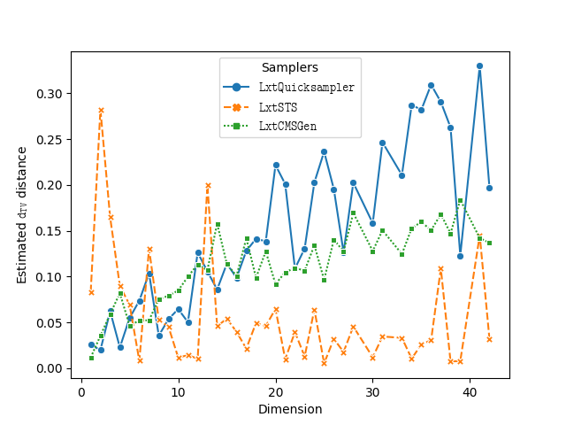
Figure 2: Estimated TV distances of samplers (from uniformity) as a function of the dimension. For each dimension, we take the median $\mathsf{d_{TV}}$ over all the instances of that dimension.

Experimental Results & Discussion

RQ1

Table 1 shows a subset of our experimental results. Due to space constraints, we have postponed presenting our comprehensive experimental results to the supplementary material. We found that among 90 instances:

• In 48 instances LxtQuickSampler has maximum $\mathsf{d_{TV}}$, in 14 instances LxtSTS has maximum $\mathsf{d_{TV}}$ distance and in 28 instances LxtCMSGen has maximum $\mathsf{d_{TV}}$ distance from uniform;

• In 10 instances LxtQuickSampler has minimum $\mathsf{d_{TV}}$ distance, in 69 instances LxtSTS has minimum $\mathsf{d_{TV}}$ distance and in 11 instances LxtCMSGen has minimum $\mathsf{d_{TV}}$ distance from uniform;

These observations indicate that LxtSTS serves as a linear extension sampler that closely resembles uniform distribution characteristics. At the same time, LxtQuickSampler deviates significantly from the traits of a uniform-like linear extension sampler. LxtCMSGen falls in an intermediate position between these two.

RQ2

Table 1 reflects that the number of samples drawn by $\mathsf{CubeProbeEst}$ depends on the dimension of an instance. Again, when the dimension is kept constant, the number of samples drawn remains similar across all runs.

RQ3

In Figure 2, we observe that for instances with lower dimensions, both LxtQuickSampler and LxtCMSGen exhibit behavior relatively close to uniform sampling. However, as the dimension increases, $\mathsf{d_{TV}}$ between these two samplers from uniformity increases. In contrast, LxtSTS shows a different behavior. In lower dimensions, the estimated $\mathsf{d_{TV}}$ distance can be notably high for certain instances, yet $\mathsf{d_{TV}}$ tends to stabilize as the dimension increases. It is worth highlighting that, in higher dimensions, LxtSTS demonstrates a more uniform-like sampling behavior compared to the other two samplers.

Conclusion

In this paper, we have designed the first self-reducible sampler tester, and used it to test linear extension samplers. We have also designed a novel variation distance estimator in the subcube-conditioning model along the way.

Limitations of our work

Our algorithm takes $\widetilde{\mathcal{O}}(n^{2})$ samples while the known lower bound for tolerant testing with subcube conditioning is of $\Omega(n/\log n)$ for this task (Canonne et al. 2020). Moreover, our algorithm works when the samplers are self-reducible, which is required for our analysis. So our algorithm can not handle non-self-reducible samplers, such as in (Große, Rothe, and Wechsung 2006; Talvitie, Vuoksenmaa, and Koivisto 2020).

SUPPLEMENTARY MATERIAL

Appendix A Probability Definitions and Useful Concentration Bounds

Definition 12 (Bernoulli distribution).

A random variable $X\in\{0,1\}$ is said to follow Bernoulli distribution with parameter $p$ if $\Pr(X=1)=p$ and $\Pr(X=0)=1-p$ for some parameter $p\in[0,1]$. This is represented as $X\sim\mathsf{Ber}(p)$.

In our work, we use the following concentration inequalities. See (Dubhashi and Panconesi 2009) for proofs.

Lemma 13 (Markov Inequality).

Let $X$ be a random variable that only takes non-negative values. Then for any $\alpha>0$, it holds that

$$\Pr(X>\alpha)\leq\frac{\mathop{\mathbb{E}}[X]}{\alpha}$$

Lemma 14 (Chernoff-Hoeffding bound).

Let $X_{1},\ldots,X_{n}$ be independent random variables such that $X_{i}\in[0,1]$. For $X=\sum\limits_{i=1}^{n}X_{i}$ and $\mu_{l}\leq\mathop{\mathbb{E}}[X]\leq\mu_{h}$, the followings hold for any $\delta>0$.

• $\Pr\left(X\geq\mu_{h}+\delta\right)\leq\exp{\left(\frac{-2\delta^{2}}{n}\right)}$.

• $\Pr\left(X\leq\mu_{l}-\delta\right)\leq\exp{\left(\frac{-2\delta^{2}}{n}\right)}$.

In the analysis of our estimator, one of the crucial components is Sub-Gaussian errors which is formally defined as follows:

Definition 15 (SubGaussian random variable (Buldygin and Kozachenko 1980)).

A random variable $X$ is said to be sub-Gaussian (SubG in short) with parameter $\alpha^{2}$ if and only if its tails are dominated by a Gaussian of parameter $\alpha^{2}$, i.e.,

$$\Pr(|X|\geq t)\leq 2\exp(-t^{2}/2\alpha^{2}),~{}~{}~{}~{}\mbox{for all }t\geq 0.$$

Lemma 16 ((Buldygin and Kozachenko 1980)).

Consider $n$ independent random variables $X_{i}\sim\mathsf{SubG}(\alpha_{i}^{2})$ for every $i\in[n]$, then

$$X_{1}+...+X_{n}\sim\mathsf{SubG}(\alpha_{1}^{2}+\alpha_{2}^{2}+\ldots+\alpha_{n}^{2})$$

We use the $\mathsf{GBAS}$ algorithm due to Huber (Huber 2017). The relevant details of the algorithm is captured by the following theorem:

Theorem 17 (Huber (Huber 2017)).

Let $\mathcal{P}$ be a Bernoulli distribution parameterised by $p$. Fix $\varepsilon\in(0,1/4)$. The randomised algorithm $\mathsf{GBAS}$   on input $k\geq\frac{3\log(2\delta^{-1})}{\varepsilon^{2}}$, samples $X_{1},X_{2},\ldots\sim\mathcal{P}$ and outputs $\widehat{p}$ after $T$ samples such that

• $\Pr\left(\left\lvert(\widehat{p}/p)-1\right\rvert>\varepsilon\right)\leq\delta$.

• $\mathop{\mathbb{E}}\left[T\right]=k/p$.

Appendix B Analysis of Estimator $\mathsf{CubeProbeEst}$

In this section we proof the correctness of $\mathsf{CubeProbeEst}$. We recall the theorem below.

Theorem 18.

Consider an unknown self-reducible sampler $\mathcal{I}_{\mathcal{G}}$, a known self-reducible sampler $\mathcal{I}_{\mathcal{W}}$, an input $\psi$, an approximation parameter $\zeta\in(0,1)$ and a confidence parameter $\delta\in(0,1)$. Our Self-reducible-sampler-tester $\mathsf{CubeProbeEst}$ is a $(\zeta,\delta)$-approx $\mathsf{d_{TV}}$ estimator and $\mathsf{CubeProbeEst}$ takes $\widetilde{\mathcal{O}}(n^{2}/\zeta^{4})$ samples.

Proof of Theorem 18

For ease of presentation, we will denote the distribution corresponding to the unknown self-reducible sampler $\mathcal{I}_{\mathcal{G}}$ on input $\psi$ as $P$ and distribution corresponding to the known self-reducible sampler $\mathcal{I}_{\mathcal{W}}$ on input $\psi$ as $Q$. We start with the correctness of $\mathsf{Est}$ .

Correctness of $\mathsf{Est}$

Let $P(x)$ be the probability mass of the distribution $P$ at the string $x\in\{0,1\}^{n}$, and $\widehat{P}(x)$ be the estimate of $P(x)$ returned by the subroutine $\mathsf{Est}$. We use $P_{i}$ to denote $P({x_{i}}\mid{x_{1}...x_{i-1}})$, the probability mass of the conditional marginal distribution considered at the index $i\in[n]$ at the string $x\in\{0,1\}^{n}$. Similarly, $\widehat{P_{i}}$ denotes the estimate of $P({x_{i}}\mid{x_{1}...x_{i-1}})$ returned by the subroutine $\mathsf{GBAS}(P\mid_{x_{1}...x_{i-1}},x_{i})$.

We define $err_{i}$ is the error in estimating the $i$-th marginal.

$$err_{i}=\left|\frac{P_{i}}{\widehat{P_{i}}}-1\right|$$ (1)

Claim 19.

Errors $err_{i}$ are SubGaussian random variables, that is, $err_{i}\sim\mathsf{SubG}\left(\frac{\gamma^{2}}{2n\log(2n/\delta^{\prime})}\right)$.

Proof.

To estimate $i$-th marginal in $\mathsf{Est}$ , the subroutine $\mathsf{GBAS}$ takes $k\geq\frac{3n}{\gamma^{2}}\cdot\log\left(\frac{2n}{\delta^{\prime}}\right)$ as input and estimates the $i$-th marginal. We have, from Theorem 17, $\Pr(|err_{i}|>\gamma/\sqrt{n})<\delta^{\prime}/n=2\exp\left(-(\gamma/\sqrt{n})^{2}\cdot\frac{n}{\gamma^{2}}\log(2n/\delta^{\prime})\right)$. So, $err_{i}\sim\mathsf{SubG}\left(\frac{\gamma^{2}}{2n\log(2n/\delta^{\prime})}\right)$. ∎

Claim 20.

Consider the random variable $err=\sum_{i=1}^{n}err_{i}$. Then we have $\Pr(|err|>\gamma)\leq\frac{\delta^{\prime}}{n}$.

Proof.

From Lemma 16, the total error in estimating is $err=\sum_{i}err_{i}\sim\mathsf{SubG}\left(\frac{\gamma^{2}}{2\log(2n/\delta^{\prime})}\right)$. By 15, we conclude that $\Pr(|err|>\gamma)\leq 2\exp(-\frac{\gamma^{2}\cdot 2\log(2n/\delta^{\prime})}{\gamma^{2}})=\frac{\delta^{\prime}}{n}$. ∎

The following lemma argues the correctness of $\mathsf{Est}$ .

Lemma 21 (Correctness of $\mathsf{Est}$ ).

Fix $\gamma,\delta\in(0,1)$. Consider $\delta^{\prime}=\frac{\delta}{2\alpha}$ for $\alpha=\frac{1}{2\zeta^{2}}\log\frac{4}{\delta}$, as fixed in the algorithms. $\mathsf{Est}$ ($P,x,\gamma/1.11,\delta^{\prime}$) estimates $P(x)$ within a multiplicative factor of $(1\pm\gamma)$ with probability at least $(1-\delta^{\prime})$, where the probability is taken over the internal randomness of $\mathsf{Est}$ . Moreover, the expected number of samples required by $\mathsf{Est}$ is $\mathcal{O}\left(\frac{n^{2}}{\gamma^{2}}\cdot\log\left(\frac{2n}{\delta^{\prime}}\right)\right)$.

Proof.

From the correctness of $\mathsf{GBAS}$ , we know that with probability at least $\delta^{\prime}/n$, the following holds for every $i\in[n]$:

$$\left|\widehat{P_{i}}-P(x_{i}|x_{1}...x_{i-1})\right|\leq\frac{\gamma}{\sqrt{n}}\cdot P(x_{i}|x_{1}...x_{i-1})$$ (2)

Therefore, from Equation 1, $err_{i}>\frac{\gamma}{\sqrt{n}}$. Taking product of above inequalities over all $i\in[n]$

$$\Pi_{i=1}^{n}\left(1-err_{i}\right)P(x)\leq\widehat{P}(x)\leq\Pi_{i=1}^{n}\left(1+err_{i}\right)P(x)$$ (3)

Assuming $err_{i}\in(0,0.8)$, we know that $1-err_{i}\geq e^{-1.11\cdot err_{i}}$ . Moreover, $(1+x)\leq e^{x}$. Thus from the above expression, we obtain a multiplicative estimate of the probability mass $P(x)$ as follows:

$$e^{-\sum_{i=1}^{n}1.11\cdot err_{i}}P(x)\leq\widehat{P}(x)\leq e^{\sum_{i=1}^{n}err_{i}}P(x)$$

Since $\sum_{i=1}^{n}err_{i}=err$, we can write the above as

$$e^{-1.11\cdot err}P(x)\leq\widehat{P}(x)\leq e^{err}P(x)$$ (4)

Now note that in the interval $x\in(0,1)$, $e^{x}\leq(1+1.11x)$ and $1-1.11x\leq e^{-1.11x}$. From 20, we know that $err\leq\gamma$ with high probability. Thus we obtain the following,

$$(1-1.11\gamma)P(x)\leq\widehat{P}(x)\leq(1+1.11\gamma)P(x)$$ (5)

Since we are calling $\mathsf{Est}(P,x,\gamma/1.11,\delta^{\prime})$, combining the above with Equation 4, we obtain a multiplicative estimate of the probability mass $P(x)$ as follows:

$$(1-\gamma)P(x)\leq\widehat{P}(x)\leq(1+\gamma)P(x)$$ (6)

To establish correctness, recall that for any index $i\in[n]$, Equation 2 fails to hold with probability at most $\delta^{\prime}/n$. Taking union bound, the error in estimating one of the $n$ marginals in Equation 4 is at most $\delta^{\prime}$.

Finally we establish the sample complexity of $\mathsf{Est}$ . To do this, we first determine the number of samples drawn by $\mathsf{GBAS}$ to estimate one marginal. Suppose $\widehat{P_{i}}$ denotes the probability mass $P_{i}=P(x_{i}\mid x_{1}...x_{i-1})$. From Theorem 17, the expected number of samples taken by $\mathsf{GBAS}$ is given by

$$\mathop{\mathbb{E}}\left(\frac{3\times 1.232n}{\gamma^{2}}\cdot\log\left(\frac{2n}{\delta^{\prime}}\right)\cdot\frac{1}{\widehat{P_{i}}}\right)$$

$$\leq \mathop{\mathbb{E}}\left(\frac{4n}{\gamma^{2}}\cdot\log\left(\frac{2n}{\delta^{\prime}}\right)\cdot\frac{1}{\widehat{P_{i}}}\right)$$

$$= \frac{4n}{\gamma^{2}}\cdot\log\left(\frac{2n}{\delta^{\prime}}\right)\left(\widehat{P}_{x_{i}=0}\cdot\frac{1}{\widehat{P}_{x_{i}=0}}+\widehat{P}_{x_{i}=1}\cdot\frac{1}{\widehat{P}_{x_{i}=1}}\right)$$

$$= \frac{8n}{\gamma^{2}}\cdot\log\left(\frac{2n}{\delta^{\prime}}\right)$$

As the $\mathsf{Est}$ calls the subroutine $\mathsf{GBAS}$ $n$ times, therefore the total expected sample complexity is given by

$$\frac{8n^{2}}{\gamma^{2}}\cdot\log\left(\frac{2n}{\delta^{\prime}}\right)$$

This concludes the proof of the claim.

∎

Claim 22.

Let $\widehat{P}(x)$ be the estimate of $P(x)$ such that $(1-\gamma)P(x)\leq\widehat{P}(x)\leq(1+\gamma)P(x)$ holds. Then $\mathop{\mathbb{E}}\limits_{x\sim P}\left[\left|\frac{Q(x)}{P(x)}-\frac{Q(x)}{\widehat{P}(x)}\right|\right]\leq\frac{\gamma}{1-\gamma}$.

Proof.

We know that $(1-\gamma)P(x)\leq\widehat{P}(x)\leq(1+\gamma)P(x)$. Hence,

$$\frac{1}{(1+\gamma)P(x)}\leq\frac{1}{\widehat{P}(x)}\leq\frac{1}{(1-\gamma)P(x)}$$

Thus we have,

$$\frac{1}{P(x)}-\frac{1}{(1-\gamma)P(x)} \leq \frac{1}{P(x)}-\frac{1}{\widehat{P}(x)}$$

$$\leq \frac{1}{P(x)}-\frac{1}{(1+\gamma)P(x)}$$

Therefore,

$$\left|\frac{1}{P(x)}-\frac{1}{\widehat{P}(x)}\right|$$

$$\leq \max\left\{\frac{\gamma}{(1-\gamma)P(x)},\frac{\gamma}{(1+\gamma)P(x)}\right\}$$

$$= \frac{\gamma}{(1-\gamma)P(x)}$$

Therefore, by multiplying $Q(x)$ on both sides and taking expectation we have,

$$\mathop{\mathbb{E}}\limits_{x\sim P}\left[\left|\frac{Q(x)}{P(x)}-\frac{Q(x)}{\widehat{P}(x)}\right|\right]\leq\frac{\gamma}{1-\gamma}\cdot\mathop{\mathbb{E}}\limits_{x\sim P}\left[\frac{Q(x)}{P(x)}\right]=\frac{\gamma}{1-\gamma}.$$

This completes the proof of the claim. ∎

Lemma 23.

$\mathsf{d_{TV}}(P,Q)=\mathop{\mathbb{E}}\limits_{x\sim P}\max\left(0,1-\frac{Q(x)}{P(x)}\right)=\mathop{\mathbb{E}}\limits_{y\sim Q}\max\left(0,1-\frac{P(y)}{Q(y)}\right)$.

Proof.

From the definitions we have

$$\mathsf{d_{TV}}(P,Q) = \sum_{x:P(x)>Q(x)}(P(x)-Q(x))$$

$$= \sum_{x:P(x)>Q(x)}P(x)\left(1-\frac{Q(x)}{P(x)}\right)$$

$$= \sum_{x}P(x)\max\left\{0,1-\frac{Q(x)}{P(x)}\right\}$$

$$= \mathop{\mathbb{E}}_{x\sim P}\max\left\{0,1-\frac{Q(x)}{P(x)}\right\}$$

Similarly, we can also say that $\mathsf{d_{TV}}(P,Q)=\mathop{\mathbb{E}}\limits_{y\sim Q}\max\left(0,1-\frac{P(y)}{Q(y)}\right)$. ∎

Correctness of $\mathsf{CubeProbeEst}$

Now we are ready to prove the correctness of $\mathsf{CubeProbeEst}$.

Lemma 24.

Let $v$ be the output of $\mathsf{CubeProbeEst}$ ($\mathcal{I}_{\mathcal{G}},\mathcal{I}_{\mathcal{W}},\psi,\zeta,\delta$). It holds, with probability at least 1-$\delta$ that

$$\mathsf{d^{\psi}_{TV}}(\mathcal{I}_{\mathcal{G}},\mathcal{I}_{\mathcal{W}})-\zeta\leq v\leq\mathsf{d^{\psi}_{TV}}(\mathcal{I}_{\mathcal{G}},\mathcal{I}_{\mathcal{W}})+\zeta$$

Proof.

From the description of Algorithm $\mathsf{CubeProbeEst}$ (Algorithm 1), $v=val/\alpha$, where $val=\sum_{i=1}^{\alpha}\max\left(0,1-\frac{Q(x)}{\widehat{P}(x)}\right)$. Recall, $\widehat{P}(x)$ denotes the estimate of $P(x)$ as returned by $\mathsf{Est}$.

Consider the event $\mathcal{A}$:

$$\mathcal{A}:=\mathsf{Est}\ \mbox{outputs a correct estimate of}\ P(x)$$

From 21, we know that $\Pr(\mathcal{A})=1-\delta^{\prime}$, where $\delta^{\prime}=\delta/2\alpha$. From now on, we work in the conditional space that the even $\mathcal{A}$ holds.

To prove the lemma, we need to prove the following:

$$\mathsf{d^{\psi}_{TV}}(\mathcal{I}_{\mathcal{G}},\mathcal{I}_{\mathcal{W}})-\zeta\leq\frac{val}{\alpha}\leq\mathsf{d^{\psi}_{TV}}(\mathcal{I}_{\mathcal{G}},\mathcal{I}_{\mathcal{W}})+\zeta$$

Case 1 Suppose $Q(x)<P(x)<\widehat{P}(x)$. Then we have $\frac{Q(x)}{\widehat{P}(x)}<\frac{Q(x)}{P(x)}<1$. Therefore using the triangle inequality, we can say the following:

$$\left|1-\frac{Q(x)}{\widehat{P}(x)}\right| \leq \left|1-\frac{Q(x)}{P(x)}\right|+\left|\frac{Q(x)}{P(x)}-\frac{Q(x)}{\widehat{P}(x)}\right|$$

$$1-\frac{Q(x)}{\widehat{P}(x)} \leq 1-\frac{Q(x)}{P(x)}+\left|\frac{Q(x)}{P(x)}-\frac{Q(x)}{\widehat{P}(x)}\right|$$

$$\max\left(0,1-\frac{Q(x)}{\widehat{P}(x)}\right) \leq \max\left(0,1-\frac{Q(x)}{P(x)}\right)$$

$$+ \left|\frac{Q(x)}{P(x)}-\frac{Q(x)}{\widehat{P}(x)}\right|$$

Case 2 Suppose $Q(x)<\widehat{P}(x)<P(x)$. Then we have $\frac{Q(x)}{P(x)}<\frac{Q(x)}{\widehat{P}(x)}<1$. Therefore using the same triangle inequality we have:

$$\left|1-\frac{Q(x)}{\widehat{P}(x)}\right| \leq \left|1-\frac{Q(x)}{P(x)}\right|+\left|\frac{Q(x)}{P(x)}-\frac{Q(x)}{\widehat{P}(x)}\right|$$

$$1-\frac{Q(x)}{\widehat{P}(x)} \leq 1-\frac{Q(x)}{P(x)}+\left|\frac{Q(x)}{P(x)}-\frac{Q(x)}{\widehat{P}(x)}\right|$$

$$\max\left(0,1-\frac{Q(x)}{\widehat{P}(x)}\right) \leq \max\left(0,1-\frac{Q(x)}{P(x)}\right)$$

$$+ \left|\frac{Q(x)}{P(x)}-\frac{Q(x)}{\widehat{P}(x)}\right|$$

Case 3 Suppose $\widehat{P}(x)<P(x)<Q(x)$ . Then using the facts that $\frac{Q(x)}{\widehat{P}(x)}>1$ and $\frac{Q(x)}{P(x)}>1$ and $\left|\frac{Q(x)}{P(x)}-\frac{Q(x)}{\widehat{P}(x)}\right|\geq 0$, we have:

$$\max\left(0,1-\frac{Q(x)}{\widehat{P}(x)}\right) \leq \max\left(0,1-\frac{Q(x)}{P(x)}\right)$$

$$+ \left|\frac{Q(x)}{P(x)}-\frac{Q(x)}{\widehat{P}(x)}\right|$$

Case 4 Suppose $P(x)<\widehat{P}(x)<Q(x)$ . Follows from the above case.

Case 5 Suppose $P(x)<Q(x)<\widehat{P}(x)$. Then using the fact $\frac{Q(x)}{P(x)}>1$ and $\frac{Q(x)}{\widehat{P}(x)}<1$, we have:

$$\left|1-\frac{Q(x)}{\widehat{P}(x)}\right| \leq \left|\frac{Q(x)}{P(x)}-\frac{Q(x)}{\widehat{P}(x)}\right|$$

$$1-\frac{Q(x)}{\widehat{P}(x)} \leq 0+\left|\frac{Q(x)}{P(x)}-\frac{Q(x)}{\widehat{P}(x)}\right|$$

$$\max\left(0,1-\frac{Q(x)}{\widehat{P}(x)}\right) \leq \max\left(0,1-\frac{Q(x)}{P(x)}\right)$$

$$+ \left|\frac{Q(x)}{P(x)}-\frac{Q(x)}{\widehat{P}(x)}\right|$$

Case 6 Suppose $\widehat{P}(x)<Q(x)<P(x)$. Then using the fact $\frac{Q(x)}{P(x)}<1$ and $\frac{Q(x)}{\widehat{P}(x)}>1$, we can say that:

$$0 \leq \left(1-\frac{Q(x)}{P(x)}\right)+\left|\frac{Q(x)}{P(x)}-\frac{Q(x)}{\widehat{P}(x)}\right|$$

$$\max\left(0,1-\frac{Q(x)}{\widehat{P}(x)}\right) \leq \max\left(0,1-\frac{Q(x)}{P(x)}\right)$$

$$+ \left|\frac{Q(x)}{P(x)}-\frac{Q(x)}{\widehat{P}(x)}\right|$$

Therefore for all $x$ we have,

$$\max\left(0,1-\frac{Q(x)}{\widehat{P}(x)}\right) \leq \max\left(0,1-\frac{Q(x)}{P(x)}\right)$$

$$+ \left|\frac{Q(x)}{P(x)}-\frac{Q(x)}{\widehat{P}(x)}\right|$$

Similarly, we also can show the following:

$$\max\left(0,1-\frac{Q(x)}{P(x)}\right) - \left|\frac{Q(x)}{P(x)}-\frac{Q(x)}{\widehat{P}(x)}\right|$$

$$\leq \max\left(0,1-\frac{Q(x)}{\widehat{P}(x)}\right)$$

Therefore taking expectation with respect to $x$ sampled from $P$ and using 22, we have the following inequality:

$$\mathsf{d_{TV}}(P,Q)-\frac{\gamma}{1-\gamma} \leq \mathop{\mathbb{E}}\limits_{x\sim P}\left[\max\left(0,1-\frac{Q(x)}{\widehat{P}(x)}\right)\right]$$

$$\leq \mathsf{d_{TV}}(P,Q)+\frac{\gamma}{1-\gamma}$$

$$\mathsf{d_{TV}}(P,Q)-\frac{\zeta}{2} \leq \mathop{\mathbb{E}}\limits_{x\sim P}\left[\max\left(0,1-\frac{Q(x)}{\widehat{P}(x)}\right)\right]$$

$$\leq \mathsf{d_{TV}}(P,Q)+\frac{\zeta}{2}$$

the last inequality follows from $\zeta=\frac{2\gamma}{1-\gamma}$. Recall that $\alpha=\frac{2}{\zeta^{2}}\log\frac{4}{\delta}$. Therefore using Chernoff-Hoeffding bound we have,

$$\Pr\left(\frac{val}{\alpha}>\mathsf{d_{TV}}(P,Q)+\zeta\right) \leq \exp\left(-\frac{\zeta^{2}\alpha^{2}}{2\alpha}\right)$$

$$\leq \frac{\delta}{4}$$

Similarly, we can prove the following:

$$\Pr\left(\frac{val}{\alpha}<\mathsf{d_{TV}}(P,Q)-\zeta\right)\leq\frac{\delta}{4}$$

Thus, under the condition that the event $\mathcal{A}$ holds, combining the above, we conclude that our algorithm outputs $\frac{val}{\alpha}\in[\mathsf{d_{TV}}(P,Q)-\zeta,\mathsf{d_{TV}}(P,Q)+\zeta]$ with probability at least $1-\frac{\delta}{2}$.

What is left is to bound the probability that $\mathcal{A}$ does not hold for some $x\in S$. Recall, from 21 for each $x$, it holds that $\Pr(\neg\mathcal{A})\leq\delta/2\alpha$. As the subroutine $\mathsf{Est}$ is called for $\alpha$ times, the probability that $\mathcal{A}$ does not hold for some $x\in S$ is at most $\delta/2$. Thus the total error of algorithm $\mathsf{CubeProbeEst}$ is bounded by $\delta$. ∎

Sample Complexity

Lemma 25.

The total sample complexity of $\mathsf{CubeProbeEst}$ is $\mathcal{O}\left(\frac{n^{2}(2+\zeta)^{2}}{\zeta^{4}}\cdot\log\left(\frac{4n\alpha}{\delta}\right)\log\frac{4}{\delta}\right)$ where $\alpha=\frac{1}{2\zeta^{2}}\log\frac{4}{\delta}$.

Proof.

From the description of the algorithm, we know $\alpha=\frac{1}{2\zeta^{2}}\log\frac{4}{\delta}$. From 21, we know that $\mathsf{Est}$ requires $\mathcal{O}\left(\frac{n^{2}}{\gamma^{2}}\cdot\log\left(\frac{2n}{\delta^{\prime}}\right)\right)$ samples on expectation in every iteration, where $\delta^{\prime}=\delta/2\alpha$ and $\gamma=\zeta/1.11(2+\zeta)$. Since $\mathsf{CubeProbeEst}$ runs $\alpha$ iterations, using Markov inequality, the total sample complexity of $\mathsf{CubeProbeEst}$ is $\mathcal{O}\left(\frac{n^{2}(2+\zeta)^{2}}{\zeta^{4}}\cdot\log\left(\frac{4n\alpha}{\delta}\right)\log\frac{4}{\delta}\right)$.

∎

Appendix C Correctness of Tester

Similar to the analysis of the estimator, for ease of presentation, we will denote the distribution corresponding to the unknown self-reducible sampler $\mathcal{I}_{\mathcal{G}}$ on input $\psi$ as $P$ and distribution corresponding to the known self-reducible sampler $\mathcal{I}_{\mathcal{W}}$ on input $\psi$ as $Q$.

Theorem 26.

Consider an unknown self-reducible sampler $\mathcal{I}_{\mathcal{G}}$, a known self-reducible sampler $\mathcal{I}_{\mathcal{W}}$, an input $\psi$, closeness parameter $\varepsilon\in(0,1)$, farness parameter $\eta\in(0,1)$ with $\eta>\varepsilon$ and a confidence parameter $\delta\in(0,1)$. There exists a $(\varepsilon,\eta,\delta)$-Self-reducible-sampler-tester $\mathsf{CubeProbeTester}$ that takes $\widetilde{\mathcal{O}}\left(n^{2}/\left(\eta-\varepsilon\right)^{4}\right)$ samples.

We will prove the correctness of $\mathsf{CubeProbeTester}$ into two parts:

• Completeness: If $\mathcal{I}_{\mathcal{G}}$ is $\varepsilon$-close to $\mathcal{I}_{\mathcal{W}}$ on input $\psi$, $\mathsf{CubeProbeTester}$ outputs ACCEPT .

• Soundness: if $\mathcal{I}_{\mathcal{G}}$ is $\eta$-far from $\mathcal{I}_{\mathcal{W}}$ on input $\psi$, $\mathsf{CubeProbeTester}$ outputs REJECT .

Proof of Completeness

Lemma 27.

Suppose $\mathcal{I}_{\mathcal{G}}$ is $\varepsilon$-close to the known self-reducible sampler $\mathcal{I}_{\mathcal{W}}$ on input $\psi$. Then $\mathsf{CubeProbeTester}$ outputs ACCEPT with probability at least $1-\delta$.

Proof of Lemma 27.

Let us first consider the event $\mathcal{A}$:

$$\mathcal{A}:=\mathsf{Est}\ \mbox{outputs a correct estimate of P(x)}$$

From 21, we know that $\Pr(\mathcal{A})=1-\delta^{\prime}$, where $\delta^{\prime}=\delta/2\alpha$. Let us now work on the conditional space that event $\mathcal{A}$ holds.

Since $\mathsf{d_{TV}}(P,Q)\leq\varepsilon$, from Lemma 23 we know that

$$\mathop{\mathbb{E}}\limits_{x\sim P}\left[\max\left(0,1-\frac{Q(x)}{P(x)}\right)\right]\leq\varepsilon$$

Therefore following the same arguments as in 23 we have

$$\mathop{\mathbb{E}}\limits_{x\sim P}\left[\max\left(0,1-\frac{Q(x)}{\widehat{P}(x)}\right)\right]\leq\varepsilon+\frac{\gamma}{1-\gamma}$$

Recall that $\frac{2\gamma}{1-\gamma}=\frac{\eta-\varepsilon}{2}$.

We derive

$$\mathop{\mathbb{E}}\limits_{x\sim P}\left[\max\left(0,1-\frac{Q(x)}{\widehat{P}(x)}\right)\right] \leq \varepsilon+\frac{(\eta-\varepsilon)}{4}=\frac{\eta+3\varepsilon}{4}$$

Recall that $K=\frac{\eta+\varepsilon}{2}$ and $\alpha=\frac{8}{(\eta-\varepsilon)^{2}}\log\left(\frac{2}{\delta}\right)$. Using the Chernoff-Hoeffding bound we have,

$$\Pr\left(\frac{val}{\alpha}>K\right) = \Pr\left(\frac{val}{\alpha}>\frac{\eta+3\varepsilon}{4}+\frac{\eta-\varepsilon}{4}\right)$$

$$\leq \exp\left(-2\left(\frac{\eta-\varepsilon}{4}\right)^{2}\cdot\alpha\right)$$

$$\leq \frac{\delta}{2}$$

Thus, under the conditional space that the event $\mathcal{A}$ holds, our algorithm accepts with probability at least $1-\frac{\delta}{2}$. Since $\Pr(\mathcal{A})\geq 1-\delta^{\prime}$ with $\delta^{\prime}=\delta/2\alpha$ and the subroutine $\mathsf{Est}$ is called for $\alpha$ times, the total error following $\mathsf{Est}$ is bounded by $\delta/2$. of our algorithm is bounded by $\alpha\cdot\delta^{\prime}+\frac{\delta}{2}$. Thus the total error of our algorithm $\mathsf{CubeProbeEst}$ is bounded by $\delta$. So we conclude that when $\mathsf{d_{TV}}(P,Q)\leq\varepsilon$, $\mathsf{CubeProbeEst}$ accepts with probability at least $1-\delta$.

∎

Proof of Soundness

Lemma 28.

Suppose $\mathcal{I}_{\mathcal{G}}$ is $\eta$-far from the known self-reducible sampler $\mathcal{I}_{\mathcal{W}}$ on input $\psi$. Then $\mathsf{CubeProbeEst}$ outputs REJECT with probability at least $1-\delta$.

Proof.

Like the completeness proof (27), we first work on the conditional space that the event $\mathcal{A}$ holds.

From the assumption, we know that $P$ and $Q$ are $\eta$-far, that is, $\mathsf{d_{TV}}(P,Q)\geq\eta$. From 23, we know that

$$\mathop{\mathbb{E}}\limits_{x\sim P}\left[\max\left(0,1-\frac{Q(x)}{P(x)}\right)\right]\geq\eta$$

Therefore following the same arguments as in 23 we have

$$\mathop{\mathbb{E}}\limits_{x\sim P}\left[\max\left(0,1-\frac{Q(x)}{\widehat{P}(x)}\right)\right]\geq\eta-\frac{\gamma}{1-\gamma}$$

Recall that $\frac{2\gamma}{1-\gamma}=\frac{\eta-\varepsilon}{2}$.

We derive

$$\mathop{\mathbb{E}}\limits_{x\sim P}\left[\max\left(0,1-\frac{Q(x)}{\widehat{P}(x)}\right)\right] \geq \eta-\frac{(\eta-\varepsilon)}{4}=\frac{3\eta+\varepsilon}{4}$$

Recall that $K=\frac{\eta+\varepsilon}{2}$ and $\alpha=\frac{8}{(\eta-\varepsilon)^{2}}\log\left(\frac{2}{\delta}\right)$. Using the Chernoff-Hoeffding bound we have,

$$\Pr\left(\frac{val}{\alpha}<K\right) = \Pr\left(\frac{val}{\alpha}<\frac{3\eta+\varepsilon}{4}-\frac{\eta-\varepsilon}{4}\right)$$

$$\leq \exp\left(-2\left(\frac{\eta-\varepsilon}{4}\right)^{2}\cdot\alpha\right)$$

$$\leq \frac{\delta}{2}$$

Thus, under the conditional space that the event $\mathcal{A}$ holds, our algorithm rejects with probability at least $1-\frac{\delta}{2}$. Since $\Pr(\mathcal{A})\geq 1-\delta^{\prime}$ with $\delta^{\prime}=\delta/2\alpha$ and the subroutine $\mathsf{Est}$ is called for $\alpha$ times, the total error following $\mathsf{Est}$ is bounded by $\delta/2$. of our algorithm is bounded by $\alpha\cdot\delta^{\prime}+\frac{\delta}{2}$. Thus the total error of our algorithm $\mathsf{CubeProbeEst}$ is bounded by $\delta$. So we conclude that when $\mathsf{d_{TV}}(P,Q)\geq\eta$, $\mathsf{CubeProbeEst}$ rejects with probability at least $1-\delta$.

∎

The sample complexity bound of $\mathsf{CubeProbeTester}$ follows from 25.

Appendix D Extended Experimental Results

In this section we describe the extended experimental results of $\mathsf{CubeProbeEst}$ and $\mathsf{CubeProbeTester}$. As mentioned in the main paper, for each instance-sampler pair, 8 cores have been employed. All the experiments have been carried out in a high-performance cluster, where each node consists of AMD EPYC 7713 CPUs with $2\times 64$ cores and 512 GB memory. Here we provide two sets of experimental results with different parameter settings.

• Experiment-1: Table 2 and Table 3 show the outcomes of Experiment-1. For the estimator $\mathsf{CubeProbeEst}$, the approximation parameter $\zeta$ is set to $0.3$, and for the tester $\mathsf{CubeProbeTester}$ the tolerance parameter $\varepsilon$ and intolerance parameter $\eta$ are set to $0.005$ and $0.605$ respectively. The experiment was run with a cutoff time of 10 hrs. The experiment ended for all instances and for all the samplers within the time-limit.

• Experiment-2: Table 4 and Table 5 show the outcomes of Experiment-2. For the estimator $\mathsf{CubeProbeEst}$, the approximation parameter $\zeta$ is set to $0.2$, and for the tester $\mathsf{CubeProbeTester}$ the tolerance parameter $\varepsilon$ and intolerance parameter $\eta$ are set to $0.005$ and $0.405$ respectively. The experiment was run with a cutoff time of 24 hours. Notably, with regard to LxtCMSGen, the experiment concluded for all but one instance. Concerning LxtQuickSampler  and LxtSTS, certain instances exceeded the time limit, denoted by "TLE" in Table 4 and Table 5.

(a)      Experiment-1

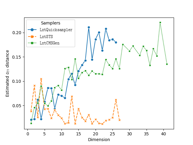
(b)      Experiment-2

Figure 3: Estimated TV distance of samplers as a function of dimension. For each dimension, we take the median $\mathsf{d_{TV}}$ over all the instances of that dimension.

The trends observed in both Figure 3(a) and Figure 3(b) consistently highlight the fact that LxtQuickSampler is significantly distant from uniform behavior and tends to perform even less effectively in scenarios involving higher dimensions. Conversely, LxtSTS demonstrates relatively satisfactory performance even as the dimensions increase.

		LxtQuickSampler			LxtSTS			LxtCMSGen
Instances	dim	Est $\mathsf{d_{TV}}$	#samples	A / R	Est $\mathsf{d_{TV}}$	#samples	A / R	Est $\mathsf{d_{TV}}$	#samples	A / R
avgdeg_3_008_0	16	0.0770	6791949	A	0.0396	6799423	A	0.1459	6755638	A
avgdeg_3_008_1	15	0.1603	6235899	A	0.0987	6384883	A	0.0916	6262721	A
avgdeg_3_008_2	19	0.1854	9986426	A	0.0205	11013078	A	0.1772	9914721	A
avgdeg_3_008_3	3	0.0241	287465	A	0.0195	285416	A	0.0774	280819	A
avgdeg_3_008_4	9	0.0474	2283299	A	0.1174	2315199	A	0.0974	2252605	A
avgdeg_3_010_0	12	0.1263	4181412	A	0.0130	4201404	A	0.1195	4197034	A
avgdeg_3_010_1	16	0.1362	7158366	A	0.0096	7127196	A	0.1050	6943720	A
avgdeg_3_010_2	30	0.1551	24537279	A	0.0155	24758147	A	0.1267	24126731	A
avgdeg_3_010_3	17	0.1096	8640869	A	0.1229	8130097	A	0.2002	8155202	A
avgdeg_3_010_4	19	0.0821	9790010	A	0.0595	9473764	A	0.0784	9408097	A
avgdeg_5_008_0	2	0.0199	130108	A	0.2822	108589	A	0.0355	130340	A
avgdeg_5_008_1	5	0.0652	754244	A	0.0693	758299	A	0.0542	743992	A
avgdeg_5_008_2	1	0.0258	38595	A	0.0832	35811	A	0.0117	39036	A
avgdeg_5_008_3	3	0.1006	288833	A	0.3098	265599	R	0.0410	293001	A
avgdeg_5_008_4	5	0.0574	791503	A	0.0578	808043	A	0.0466	783762	A
avgdeg_5_010_0	5	0.0172	712465	A	0.1637	676270	A	0.0295	705167	A
avgdeg_5_010_1	10	0.0913	2911946	A	0.0029	3002641	A	0.0751	2892695	A
avgdeg_5_010_2	10	0.0647	2989504	A	0.0117	3126246	A	0.0869	2926277	A
avgdeg_5_010_3	16	0.0976	7593533	A	0.0338	7338508	A	0.1135	7261255	A
avgdeg_5_010_4	11	0.0503	3486025	A	0.0387	3475635	A	0.1147	3412151	A
bn_andes_008_0	9	0.0546	2286676	A	0.0581	2170358	A	0.1070	2217610	A
bn_andes_008_1	5	0.0272	745159	A	0.1264	716324	A	0.0489	742531	A
bn_andes_008_2	17	0.1323	8109742	A	0.0052	8160580	A	0.0898	7913759	A
bn_andes_008_3	17	0.1027	7550199	A	0.0796	7545288	A	0.1707	7490279	A
bn_andes_008_4	6	0.0888	1118383	A	0.0000	1142299	A	0.0504	1109175	A
bn_andes_010_0	31	0.1373	26115828	A	0.0258	25906414	A	0.1441	25618332	A
bn_andes_010_1	35	0.2742	33557190	A	0.0396	33536595	A	0.1601	33235104	A
bn_andes_010_2	30	0.1615	23482099	A	0.0321	24970138	A	0.1082	24027291	A
bn_andes_010_3	22	0.1162	13214113	A	0.0323	12519139	A	0.1132	12754238	A
bn_andes_010_4	30	0.1479	24040660	A	0.0010	23654061	A	0.1344	23805848	A
bn_diabetes_008_0	5	0.0549	746520	A	0.0562	767293	A	0.0449	727519	A
bn_diabetes_008_1	10	0.0402	2776787	A	0.0278	2693513	A	0.0849	2724153	A
bn_diabetes_008_2	9	0.0233	2184696	A	0.0358	2272086	A	0.0484	2161198	A
bn_diabetes_008_3	11	0.0650	3328170	A	0.0014	3497447	A	0.1000	3275040	A
bn_diabetes_008_4	8	0.0357	1839552	A	0.0530	1850440	A	0.0754	1781282	A
bn_diabetes_010_0	4	0.0228	465532	A	0.0898	451759	A	0.0820	450749	A
bn_diabetes_010_1	9	0.0222	2245072	A	0.0080	2242919	A	0.0792	2207156	A
bn_diabetes_010_2	9	0.0536	2378066	A	0.0291	2368284	A	0.1257	2261017	A
bn_diabetes_010_3	26	0.1955	19211200	A	0.0009	18847561	A	0.1478	18539480	A
bn_diabetes_010_4	14	0.0860	5649464	A	0.0524	5691881	A	0.1639	5422008	A
bn_link_008_0	9	0.0842	2226961	A	0.0453	2277521	A	0.0691	2207517	A
bn_link_008_1	13	0.1057	4797656	A	0.1695	4703993	A	0.0921	4770505	A
bn_link_008_2	16	0.0477	6743323	A	0.1656	6598629	A	0.1030	6691303	A
bn_link_008_3	18	0.0897	9022112	A	0.0503	8548411	A	0.0966	8753456	A
bn_link_008_4	9	0.0591	2373720	A	0.0511	2327557	A	0.0596	2319283	A
bn_link_010_0	17	0.1570	8390237	A	0.0860	8460641	A	0.1657	8139453	A
bn_link_010_1	22	0.0990	14164767	A	0.0827	13518741	A	0.1213	13543042	A
bn_link_010_2	31	0.2622	27296306	A	0.0392	26956958	A	0.1870	26428380	A
bn_link_010_3	23	0.1307	14754743	A	0.0122	14717663	A	0.1057	14582464	A

Table 2: Extended table of Experiment-1: for each sampler the three columns represent the estimated $\mathsf{d_{TV}}$, number of samples consumed by $\mathsf{CubeProbeEst}$, and the output of $\mathsf{CubeProbeTester}$. “A” and “R” represents ACCEPT and REJECT respectively.

		LxtQuickSampler			LxtSTS			LxtCMSGen
Instances	dim	Est $\mathsf{d_{TV}}$	#samples	A / R	Est $\mathsf{d_{TV}}$	#samples	A / R	Est $\mathsf{d_{TV}}$	#samples	A / R
bn_link_010_4	28	0.2024	21482230	A	0.0346	22377750	A	0.1635	21161624	A
bn_munin_008_0	20	0.1772	11426488	A	0.0831	11433681	A	0.0741	11279783	A
bn_munin_008_1	17	0.1434	8322983	A	0.0223	7988525	A	0.1431	8073056	A
bn_munin_008_2	7	0.1037	1541062	A	0.1305	1541043	A	0.0524	1538649	A
bn_munin_008_3	11	0.0295	3218909	A	0.0144	3283721	A	0.0703	3169267	A
bn_munin_008_4	16	0.1046	7542041	A	0.0758	7318602	A	0.0551	7366044	A
bn_munin_010_0	22	0.1014	13317551	A	0.0031	13771779	A	0.0866	13227172	A
bn_munin_010_1	33	0.2414	30348931	A	0.0448	30693619	A	0.1230	30218998	A
bn_munin_010_2	16	0.0998	7467635	A	0.0349	7304639	A	0.0884	7302971	A
bn_munin_010_3	27	0.1035	21146390	A	0.0385	20982832	A	0.1197	20674124	A
bn_munin_010_4	31	0.2309	26817254	A	0.0068	28253865	A	0.1501	26738535	A
bn_pigs_008_0	15	0.0680	6441942	A	0.0095	6461249	A	0.1307	6396630	A
bn_pigs_008_1	17	0.1281	7774163	A	0.0191	7933187	A	0.0985	7728098	A
bn_pigs_008_2	6	0.0587	1123099	A	0.0167	1101813	A	0.0540	1110811	A
bn_pigs_008_3	19	0.0992	9948699	A	0.0618	10059015	A	0.1072	9760731	A
bn_pigs_008_4	17	0.1075	7925545	A	0.0124	8339326	A	0.1228	7944301	A
bn_pigs_010_0	25	0.1522	17232391	A	0.0194	17165983	A	0.1079	17177624	A
bn_pigs_010_1	36	0.3106	36917129	R	0.0569	36311963	A	0.1353	35978964	A
bn_pigs_010_2	26	0.0840	18271388	A	0.0379	17871066	A	0.1416	17918820	A
bn_pigs_010_3	21	0.1797	12416175	A	0.0237	12564348	A	0.0900	12311760	A
bn_pigs_010_4	33	0.1801	29035557	A	0.0425	28940748	A	0.1397	29062723	A
bipartite_0.2_008_0	27	0.1494	21251509	A	0.0009	20872703	A	0.1392	20643211	A
bipartite_0.2_008_1	24	0.1718	15831995	A	0.0773	15584683	A	0.1687	15744980	A
bipartite_0.2_008_2	24	0.2339	16551565	A	0.0524	16834575	A	0.0984	16167092	A
bipartite_0.2_008_3	26	0.2624	19225000	A	0.0490	19291040	A	0.1292	19010387	A
bipartite_0.2_008_4	25	0.3204	17761820	R	0.0073	17840945	A	0.1153	17546682	A
bipartite_0.2_010_0	42	0.1970	49798327	A	0.0326	50031620	A	0.1373	49064133	A
bipartite_0.2_010_1	41	0.3299	46244946	R	0.1528	48135745	A	0.1461	47003971	A
bipartite_0.2_010_2	38	0.2628	40290722	A	0.0050	39052923	A	0.1410	39715820	A
bipartite_0.2_010_3	39	0.1229	41908526	A	0.0089	43320033	A	0.1854	41380532	A
bipartite_0.2_010_4	37	0.2906	36887531	A	0.1144	38387209	A	0.1719	36703039	A
bipartite_0.5_008_0	20	0.2661	11163495	A	0.0466	11181243	A	0.1295	11075947	A
bipartite_0.5_008_1	21	0.2224	12195197	A	0.0090	12568389	A	0.1258	12246222	A
bipartite_0.5_008_2	19	0.1778	10323613	A	0.0327	10041072	A	0.1308	10061879	A
bipartite_0.5_008_3	18	0.1929	9157458	A	0.0253	9046275	A	0.0983	9174123	A
bipartite_0.5_008_4	22	0.2977	13144132	A	0.0528	13424946	A	0.1059	13317859	A
bipartite_0.5_010_0	31	0.2752	26488712	A	0.1396	27033012	A	0.1379	26555928	A
bipartite_0.5_010_1	36	0.3082	35875122	R	0.0037	36728064	A	0.1472	35823878	A
bipartite_0.5_010_2	30	0.2950	24656885	A	0.0318	25234171	A	0.1763	24946104	A
bipartite_0.5_010_3	35	0.2899	33364949	A	0.0041	34652088	A	0.1495	33144588	A
bipartite_0.5_010_4	34	0.2872	31701978	A	0.0136	33016841	A	0.1621	31255277	A

Table 3: Extended table of Experiment-1: for each sampler the three columns represent the estimated $\mathsf{d_{TV}}$, number of samples consumed by $\mathsf{CubeProbeEst}$, and the output of $\mathsf{CubeProbeTester}$. “A” and “R” represents ACCEPT and REJECT respectively.

		LxtQuickSampler			LxtSTS			LxtCMSGen
Instances	dim	Est dTV	#samples	A / R	Est dTV	#samples	A / R	Est dTV	#samples	A / R
avgdeg_3_008_0	16	0.1039	57780610	A	0.0138	58313012	A	0.1878	56107260	A
avgdeg_3_008_1	15	0.1131	53251513	A	0.0538	53541132	A	0.0983	53016623	A
avgdeg_3_008_2	19	0.1677	85093433	A	0.0149	93032499	A	0.2069	82702207	R
avgdeg_3_008_3	3	0.0320	2275994	A	0.0217	2256186	A	0.0679	2211866	A
avgdeg_3_008_4	9	0.0759	18789585	A	0.0365	19151573	A	0.0936	18843236	A
avgdeg_3_010_0	12	0.1042	35685841	A	0.0146	35364607	A	0.1285	35316610	A
avgdeg_3_010_1	16	0.1593	59077244	A	0.0209	59353049	A	0.1095	58577572	A
avgdeg_3_010_2	30	TLE		TLE	TLE		TLE	0.1415	207074074	A
avgdeg_3_010_3	17	0.1627	69823682	A	0.0359	72557219	A	0.2024	68938123	A
avgdeg_3_010_4	19	0.1191	82898928	A	0.0025	82544372	A	0.0983	80183214	A
avgdeg_5_008_0	2	0.0219	980431	A	0.0908	927524	A	0.0458	970055	A
avgdeg_5_008_1	5	0.0617	6124907	A	0.0429	6228781	A	0.0693	6026403	A
avgdeg_5_008_2	1	0.0209	265167	A	0.0382	258241	A	0.0133	265950	A
avgdeg_5_008_3	3	0.0923	2320436	A	0.0305	2384329	A	0.0419	2297683	A
avgdeg_5_008_4	5	0.0793	6482679	A	0.0555	6525853	A	0.0571	6389508	A
avgdeg_5_010_0	5	0.0365	5743370	A	0.0468	5674007	A	0.0243	5742673	A
avgdeg_5_010_1	10	0.1132	24020823	A	0.0404	24484289	A	0.0817	24137189	A
avgdeg_5_010_2	10	0.0699	24747864	A	0.0242	26095975	A	0.0801	24456664	A
avgdeg_5_010_3	16	0.1233	63074585	A	0.0300	62222499	A	0.1401	61604767	A
avgdeg_5_010_4	11	0.0803	29102997	A	0.0127	29124086	A	0.1333	28654516	A
bn_andes_008_0	9	0.0726	19023793	A	0.0380	18562663	A	0.1119	18506030	A
bn_andes_008_1	5	0.0426	6058830	A	0.0197	5982108	A	0.0542	6030187	A
bn_andes_008_2	17	0.1429	68238367	A	0.0085	69118136	A	0.1025	67180255	A
bn_andes_008_3	17	0.1115	64243462	A	0.0145	64199971	A	0.1758	63631988	A
bn_andes_008_4	6	0.0892	9120656	A	0.0618	9093011	A	0.0499	9081693	A
bn_andes_010_0	31	TLE		TLE	TLE		TLE	0.1722	220087159	A
bn_andes_010_1	35	TLE		TLE	TLE		TLE	0.1756	284427541	A
bn_andes_010_2	30	TLE		TLE	TLE		TLE	0.1634	204364382	A
bn_andes_010_3	22	0.1513	109527008	A	0.0184	107994462	A	0.1145	109098691	A
bn_andes_010_4	30	TLE		TLE	TLE		TLE	0.1609	204468940	A
bn_diabetes_008_0	5	0.0577	5995874	A	0.0118	6095489	A	0.0525	5932073	A
bn_diabetes_008_1	10	0.0593	22902385	A	0.0149	22847974	A	0.0971	22777546	A
bn_diabetes_008_2	9	0.0308	18512750	A	0.0117	18802383	A	0.0681	17974379	A
bn_diabetes_008_3	11	0.0654	27257434	A	0.0188	28549056	A	0.1258	27439919	A
bn_diabetes_008_4	8	0.0432	15207959	A	0.0408	15610670	A	0.0866	14831210	A
bn_diabetes_010_0	4	0.0222	3714311	A	0.1050	3476870	A	0.0898	3619811	A
bn_diabetes_010_1	9	0.0386	18423058	A	0.0448	18209476	A	0.0754	18392023	A
bn_diabetes_010_2	9	0.0478	19452405	A	0.0163	18903321	A	0.1227	18748501	A
bn_diabetes_010_3	26	0.1435	161376730	A	0.0070	156798964	A	0.1536	158995632	A
bn_diabetes_010_4	14	0.0923	46476806	A	0.0130	46569709	A	0.1460	44970096	A
bn_link_008_0	9	0.0827	18594762	A	0.0304	18563030	A	0.0825	18401170	A
bn_link_008_1	13	0.1152	40145648	A	0.0689	40033555	A	0.1033	40196470	A
bn_link_008_2	16	0.1002	56640105	A	0.0330	56536367	A	0.1264	56701124	A
bn_link_008_3	18	0.1638	74689794	A	0.0383	80407821	A	0.1170	74465855	A
bn_link_008_4	9	0.0895	19649837	A	0.0254	19991636	A	0.0913	19395181	A
bn_link_010_0	17	0.2041	70341646	A	0.0478	73798615	A	0.1548	69806129	A
bn_link_010_1	22	0.1751	119908947	A	0.0138	117058259	A	0.1135	116693457	A
bn_link_010_2	31	TLE		TLE	TLE		TLE	0.1725	221320283	A
bn_link_010_3	23	0.2078	124171660	R	0.0190	125714245	A	0.1443	124789269	A
bn_link_010_4	28	TLE		TLE	TLE		TLE	0.1759	181566146	A

Table 4: Table of Experiment-2: for each sampler the three columns represent the estimated $\mathsf{d_{TV}}$, number of samples consumed by $\mathsf{CubeProbeEst}$, and the output of $\mathsf{CubeProbeTester}$. “A” and “R” represents ACCEPT and REJECT respectively. “TLE” indicates “Time limit exceeded”.

		LxtQuickSampler			LxtSTS			LxtCMSGen
Instances	dim	Est $\mathsf{d_{TV}}$	#samples	A / R	Est $\mathsf{d_{TV}}$	#samples	A / R	Est $\mathsf{d_{TV}}$	#samples	A / R
bn_munin_008_0	20	TLE		TLE	0.0290	97911223	A	0.1058	95117302	A
bn_munin_008_1	17	0.1201	68388967	A	0.0133	70664348	A	0.1218	68691968	A
bn_munin_008_2	7	0.0856	13039482	A	0.0240	12770555	A	0.0596	12703958	A
bn_munin_008_3	11	0.0495	27026050	A	0.0103	26869725	A	0.0954	26727097	A
bn_munin_008_4	16	0.1429	63190585	A	0.0316	62557467	A	0.0671	62407076	A
bn_munin_010_0	22	0.1371	112112573	A	0.0010	115964692	A	0.1102	112190751	A
bn_munin_010_1	33	TLE		TLE	TLE		TLE	0.1314	259890442	A
bn_munin_010_2	16	0.1747	62004639	A	0.0099	61749551	A	0.0989	61675184	A
bn_munin_010_3	27	TLE		TLE	TLE		TLE	0.1327	177003733	A
bn_munin_010_4	31	TLE		TLE	TLE		TLE	0.1574	229365833	A
bn_pigs_008_0	15	0.1283	53555868	A	0.0328	53333685	A	0.1142	52302677	A
bn_pigs_008_1	17	0.1444	66393846	A	0.0272	67517048	A	0.1160	65638945	A
bn_pigs_008_2	6	0.0834	9245390	A	0.0244	9068329	A	0.0489	9090393	A
bn_pigs_008_3	19	0.1213	83142808	A	0.0111	89524401	A	0.1237	82978698	A
bn_pigs_008_4	17	0.1086	68933882	A	0.0179	70099962	A	0.1188	67407519	A
bn_pigs_010_0	25	0.1156	149629089	A	0.0323	147814237	A	0.1323	146907542	A
bn_pigs_010_1	36	TLE		TLE	TLE		TLE	0.1160	308753902	A
bn_pigs_010_2	26	TLE		TLE	0.0702	151778298	A	0.1461	153478165	A
bn_pigs_010_3	21	0.2016	106092965	A	0.0163	105320627	A	0.1058	105116805	A
bn_pigs_010_4	33	TLE		TLE	TLE		TLE	0.1747	251854250	A
bipartite_0.2_008_0	27	TLE		TLE	0.0205	177791342	A	0.1192	176767014	A
bipartite_0.2_008_1	24	0.1965	137749199	A	0.0045	135359186	A	0.1623	133916158	A
bipartite_0.2_008_2	24	0.1716	141073803	A	0.0377	141754903	A	0.1042	138303430	A
bipartite_0.2_008_3	26	0.2171	164289521	R	0.0618	163778645	A	0.1240	162976810	A
bipartite_0.2_008_4	25	0.2565	151106526	R	0.0176	153552203	A	0.1193	148516451	A
bipartite_0.2_010_0	42	TLE		TLE	TLE		TLE	TLE		TLE
bipartite_0.2_010_1	41	TLE		TLE	TLE		TLE	0.1352	396304400	A
bipartite_0.2_010_2	38	TLE		TLE	TLE		TLE	0.1523	340117827	A
bipartite_0.2_010_3	39	TLE		TLE	TLE		TLE	0.2208	356789335	R
bipartite_0.2_010_4	37	TLE		TLE	TLE		TLE	0.1666	316213957	A
bipartite_0.5_008_0	20	0.1864	96812156	A	0.0141	96811537	A	0.1245	93884621	A
bipartite_0.5_008_1	21	0.1992	104470069	A	0.0110	106252427	A	0.1244	104223715	A
bipartite_0.5_008_2	19	0.2284	85454622	R	0.0224	85876067	A	0.1181	85216406	A
bipartite_0.5_008_3	18	0.2583	77466770	R	0.0236	78003744	A	0.1074	77881493	A
bipartite_0.5_008_4	22	0.3614	112182650	R	0.0101	114351630	A	0.1150	113745999	A
bipartite_0.5_010_0	31	TLE		TLE	TLE		TLE	0.1762	226661387	A
bipartite_0.5_010_1	36	TLE		TLE	TLE		TLE	0.1490	308611030	A
bipartite_0.5_010_2	30	TLE		TLE	TLE		TLE	0.1855	212852423	A
bipartite_0.5_010_3	35	TLE		TLE	TLE		TLE	0.1506	285159013	A
bipartite_0.5_010_4	34	TLE		TLE	TLE		TLE	0.1722	267687700	A

Table 5: Table of Experiment-2: for each sampler the three columns represent the estimated $\mathsf{d_{TV}}$, number of samples consumed by $\mathsf{CubeProbeEst}$, and the output of $\mathsf{CubeProbeTester}$. “A” and “R” represents ACCEPT and REJECT respectively. “TLE” indicates “Time limit exceeded”.

References

- Andrieu et al. (2003) Andrieu, C.; De Freitas, N.; Doucet, A.; and Jordan, M. I. 2003. An introduction to MCMC for machine learning. Machine Learning.
- Ashur, De Witte, and Liu (2017) Ashur, T.; De Witte, G.; and Liu, Y. 2017. An automated tool for rotational-xor cryptanalysis of arx-based primitives. In SITB.
- Banerjee et al. (2023) Banerjee, A.; Chakraborty, S.; Chakraborty, S.; Meel, K. S.; Sarkar, U.; and Sen, S. 2023. Testing of Horn Samplers. In AISTATS.
- Bhattacharyya and Chakraborty (2018) Bhattacharyya, R.; and Chakraborty, S. 2018. Property testing of joint distributions using conditional samples. ACM Transactions on Computation Theory (TOCT).
- Blanca et al. (2023) Blanca, A.; Chen, Z.; Štefankovič, D.; and Vigoda, E. 2023. Complexity of High-Dimensional Identity Testing with Coordinate Conditional Sampling. In COLT.
- Brooks et al. (2011) Brooks, S.; Gelman, A.; Jones, G.; and Meng, X.-L. 2011. Handbook of markov chain monte carlo. Cambridge University Press.
- Buldygin and Kozachenko (1980) Buldygin, V. V.; and Kozachenko, Y. V. 1980. Sub-Gaussian random variables. Ukrainian Mathematical Journal.
- Canonne et al. (2021) Canonne, C. L.; Chen, X.; Kamath, G.; Levi, A.; and Waingarten, E. 2021. Random restrictions of high dimensional distributions and uniformity testing with subcube conditioning. In SODA.
- Canonne et al. (2020) Canonne, C. L.; Diakonikolas, I.; Kane, D. M.; and Stewart, A. 2020. Testing bayesian networks. IEEE Transactions on Information Theory.
- Canonne, Ron, and Servedio (2015) Canonne, C. L.; Ron, D.; and Servedio, R. A. 2015. Testing probability distributions using conditional samples. SIAM Journal on Computing.
- Chakraborty et al. (2016) Chakraborty, S.; Fischer, E.; Goldhirsh, Y.; and Matsliah, A. 2016. On the power of conditional samples in distribution testing. SIAM Journal on Computing.
- Chakraborty et al. (2014) Chakraborty, S.; Fremont, D.; Meel, K.; Seshia, S.; and Vardi, M. 2014. Distribution-aware sampling and weighted model counting for SAT. In AAAI.
- Chakraborty and Meel (2019) Chakraborty, S.; and Meel, K. S. 2019. On testing of uniform samplers. In AAAI.
- Chakraborty, Meel, and Vardi (2013) Chakraborty, S.; Meel, K. S.; and Vardi, M. Y. 2013. A scalable and nearly uniform generator of SAT witnesses. In ICCAD.
- Chandra and Iyengar (1992) Chandra, A. K.; and Iyengar, V. S. 1992. Constraint solving for test case generation: a technique for high-level design verification. In ICCD.
- Chen et al. (2021) Chen, X.; Jayaram, R.; Levi, A.; and Waingarten, E. 2021. Learning and testing junta distributions with sub cube conditioning. In COLT.
- Chen and Marcussen (2023) Chen, X.; and Marcussen, C. 2023. Uniformity Testing over Hypergrids with Subcube Conditioning.
- Diakonikolas et al. (2007) Diakonikolas, I.; Lee, H. K.; Matulef, K.; Onak, K.; Rubinfeld, R.; Servedio, R. A.; and Wan, A. 2007. Testing for concise representations. In FOCS.
- Dubhashi and Panconesi (2009) Dubhashi, D. P.; and Panconesi, A. 2009. Concentration of Measure for the Analysis of Randomized Algorithms. Cambridge University Press.
- Dutra et al. (2018) Dutra, R.; Laeufer, K.; Bachrach, J.; and Sen, K. 2018. Efficient sampling of SAT solutions for testing. In ICSE.
- Elidan (1998) Elidan, G. 1998. Bayesian-Network-Repository. cs.huji.ac.il/w-galel/Repository/.
- Ermon et al. (2013) Ermon, S.; Gomes, C. P.; Sabharwal, A.; and Selman, B. 2013. Embed and project: Discrete sampling with universal hashing. NeurIPS.
- Ermon, Gomes, and Selman (2012) Ermon, S.; Gomes, C. P.; and Selman, B. 2012. Uniform Solution Sampling Using a Constraint Solver As an Oracle. In UAI.
- Fotakis, Kalavasis, and Tzamos (2020) Fotakis, D.; Kalavasis, A.; and Tzamos, C. 2020. Efficient parameter estimation of truncated boolean product distributions. In COLT.
- Golia et al. (2021) Golia, P.; Soos, M.; Chakraborty, S.; and Meel, K. S. 2021. Designing samplers is easy: The boon of testers. In FMCAD.
- Gopalan et al. (2009) Gopalan, P.; O’Donnell, R.; Servedio, R. A.; Shpilka, A.; and Wimmer, K. 2009. Testing Fourier Dimensionality and Sparsity. In ICALP.
- Große, Rothe, and Wechsung (2006) Große, A.; Rothe, J.; and Wechsung, G. 2006. On computing the smallest four-coloring of planar graphs and non-self-reducible sets in P. Information Processing Letters.
- Huber (2014) Huber, M. 2014. Near-linear time simulation of linear extensions of a height-2 poset with bounded interaction. Chicago Journal of Theoretical Computer Science.
- Huber (2017) Huber, M. 2017. A Bernoulli mean estimate with known relative error distribution. Random Struct. Algorithms.
- Jerrum (1998) Jerrum, M. 1998. Mathematical foundations of the Markov chain Monte Carlo method. In Probabilistic methods for algorithmic discrete mathematics.
- Jerrum, Valiant, and Vazirani (1986) Jerrum, M. R.; Valiant, L. G.; and Vazirani, V. V. 1986. Random generation of combinatorial structures from a uniform distribution. Theoretical Computer Science.
- Khuller and Vazirani (1991) Khuller, S.; and Vazirani, V. V. 1991. Planar graph coloring is not self-reducible, assuming P NP. Theoretical Computer Science.
- Korhonen and Järvisalo (2021) Korhonen, T.; and Järvisalo, M. 2021. SharpSAT-TD Participating in Model Counting Competition 2021.
- Kumar, Meel, and Pote (2023) Kumar, G.; Meel, K. S.; and Pote, Y. 2023. Tolerant Testing of High-Dimensional Samplers with Subcube Conditioning. arXiv:2308.04264.
- Lukasiewicz, Martinez, and Simari (2014) Lukasiewicz, T.; Martinez, M. V.; and Simari, G. I. 2014. Probabilistic preference logic networks. In ECAI.
- Mahajan et al. (2023) Mahajan, G.; Kakade, S.; Krishnamurthy, A.; and Zhang, C. 2023. Learning Hidden Markov Models Using Conditional Samples. In COLT.
- Mannila and Meek (2000) Mannila, H.; and Meek, C. 2000. Global partial orders from sequential data. In SIGKDD.
- Meel, Pote, and Chakraborty (2020) Meel, K. S.; Pote, Y. P.; and Chakraborty, S. 2020. On testing of samplers. NeurIPS.
- Meel et al. (2016) Meel, K. S.; Vardi, M. Y.; Chakraborty, S.; Fremont, D. J.; Seshia, S. A.; Fried, D.; Ivrii, A.; and Malik, S. 2016. Constrained Sampling and Counting: Universal Hashing Meets SAT Solving. In Beyond NP, Papers from the 2016 AAAI Workshop, AAAI.
- Mironov and Zhang (2006) Mironov, I.; and Zhang, L. 2006. Applications of SAT solvers to cryptanalysis of hash functions. In SAT.
- Morawiecki and Srebrny (2013) Morawiecki, P.; and Srebrny, M. 2013. A SAT-based preimage analysis of reduced Keccak hash functions. Information Processing Letters.
- Morton et al. (2009) Morton, J.; Pachter, L.; Shiu, A.; Sturmfels, B.; and Wienand, O. 2009. Convex rank tests and semigraphoids. SIAM Journal on Discrete Mathematics.
- Muise, Beck, and McIlraith (2016) Muise, C.; Beck, J. C.; and McIlraith, S. A. 2016. Optimal partial-order plan relaxation via MaxSAT. Journal of Artificial Intelligence Research.
- Naveh et al. (2006) Naveh, Y.; Rimon, M.; Jaeger, I.; Katz, Y.; Vinov, M.; s Marcu, E.; and Shurek, G. 2006. Constraint-based random stimuli generation for hardware verification.
- Paninski (2008) Paninski, L. 2008. A Coincidence-Based Test for Uniformity Given Very Sparsely Sampled Discrete Data. IEEE Transactions on Information Theory.
- Peczarski (2004) Peczarski, M. 2004. New results in minimum-comparison sorting. Algorithmica.
- Pote and Meel (2022) Pote, Y.; and Meel, K. S. 2022. On Scalable Testing of Samplers. NeurIPS.
- Pote and Meel (2021) Pote, Y. P.; and Meel, K. S. 2021. Testing probabilistic circuits. NeurIPS.
- Servedio (2010) Servedio, R. A. 2010. Testing by implicit learning: a brief survey. Property Testing.
- Soos, Nohl, and Castelluccia (2009) Soos, M.; Nohl, K.; and Castelluccia, C. 2009. Extending SAT solvers to cryptographic problems. In SAT.
- Talvitie et al. (2018a) Talvitie, T.; Kangas, J.-K.; Niinimäki, T.; and Koivisto, M. 2018a. A scalable scheme for counting linear extensions. In IJCAI.
- Talvitie et al. (2018b) Talvitie, T.; Kangas, K.; Niinimäki, T.; and Koivisto, M. 2018b. Counting linear extensions in practice: MCMC versus exponential Monte Carlo. In AAAI.
- Talvitie, Vuoksenmaa, and Koivisto (2020) Talvitie, T.; Vuoksenmaa, A.; and Koivisto, M. 2020. Exact sampling of directed acyclic graphs from modular distributions. In UAI.
- Wallace, Korb, and Dai (1996) Wallace, C.; Korb, K. B.; and Dai, H. 1996. Causal discovery via MML. In ICML.
- Yuan et al. (2004) Yuan, J.; Aziz, A.; Pixley, C.; and Albin, K. 2004. Simplifying boolean constraint solving for random simulation-vector generation. IEEE Trans. Comput. Aided Des. Integr. Circuits Syst.