Data Contamination Issues in Brain-to-Text Decoding

Abstract

Decoding non-invasive cognitive signals to natural language has long been the goal of building practical brain-computer interfaces (BCIs). Recent major milestones have successfully decoded cognitive signals like functional Magnetic Resonance Imaging (fMRI) and electroencephalogram (EEG) into text under open vocabulary setting. However, how to split the datasets for training, validating, and testing in brain-to-text decoding still remains controversial. In this paper, we conduct systematic analysis on current dataset splitting methods and find data contamination largely exaggerates model performance. Specifically, first we find the leakage of test subjects’ cognitive signals corrupts the training of a robust encoder. Second, we prove the leakage of text stimuli causes the auto-regressive decoder to memorize seen information in test set. To eliminate the influence of data contamination and fairly evaluate different models’ generalization ability, we propose a new splitting method for different types of cognitive dataset (e.g. fMRI, EEG). We also test the performance of SOTA brain-to-text decoding models under the proposed dataset splitting paradigm as baselines for further research.

1 Introduction

Brain-computer interface (BCI) builds connections between human brain and external devices (e.g. computer). It has been widely researched in the field of neuroscience and has gained remarkable success like repairing damaged sight or restoring movement of disabled people (Polikov et al., 2005; Hochberg et al., 2012; Bouton et al., 2016). However, it’s still challenging in decoding cognitive signals to corresponding natural language when subjects read or hear text stimuli, especially for non-invasive cognitive signals like functional Magnetic Resonance Imaging (fMRI) or electroencephalogram (EEG) that are noisy and of low resolution (Mridha et al., 2021).

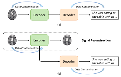
Figure 1: General frameworks of brain-to-text decoding and possible situations of data contamination.

Recent methods (Makin et al., 2020; Wang and Ji, 2022; Xi et al., 2023; Tang et al., 2023) typically viewed brain-to-text decoding as machine translation (Sutskever et al., 2014; Bahdanau et al., 2015) and adopted an encoder-decoder framework, where the encoder is responsible for converting cognitive signals into low-dimensional representations and the decoder learns to map the representations to natural language. Specifically, as shown in Figure1, the encoder usually consists of a spatial and time series feature extractor. It can be trained either in an end-to-end manner with decoder (Figure 1 a) or first pre-trained through a signal reconstruction task and then applied in decoder training (Figure 1 b). Despite recent success in model design, it still remains controversial in how to split the dataset for training, validating, and testing (Xi et al., 2023). Addressing this issue is urgent and meaningful, as fair evaluation of models is impossible without a widely recognized dataset splitting paradigm.

A cognitive dataset is usually formatted in signal-sentence pair. In most cases for brain-to-text decoding task, each sentence belongs to a certain task, so signal-sentence pair can be further divided into signal-task and task-sentence pair. Current dataset splitting methods (Wang and Ji, 2022; Xi et al., 2023) can be summarized into five categories: (1) split by subjects, (2) split by tasks, (3) split by randomly picking signal frames, (4) split by randomly picking signal frames under certain task, (5) split by randomly picking consecutive signal frames under certain task. However, all these methods suffer from data contamination on encoder side, decoder side, or both. As shown in Figure 1, to encoder if subjects’ cognitive signals in test set are mixed into training set, encoder will become overfitted and fail to well represent unseen subjects’ cognitive signals. As to decoder, situation gets worse if text stimuli are leaked. Since the decoder generates token by token in an auto-regressive manner, data contamination will cause the decoder to memorize seen paragraphs and probability distribution, which means given the first few tokens the decoder is able to predict next token regardless of encoded cognitive signal representations.

To address the above-mentioned problems, we propose a new dataset splitting method that eradicates data contamination from both encoder and decoder sides. We focus on fMRI and EEG signals in experiments, although the proposed splitting method could be applied to any cognitive signals satisfying the given format. In our method, the dataset is split according to subject-stimuli pairs with the following rules: (1) Cognitive signals collected from subjects in validation set and test set won’t appear in training set, which means the trained encoder can’t get access to any brain information belonging to subjects in test set. (2) Text stimuli in validation set and test set won’t appear in training set. The decoder learns the mapping between cognitive signal representation and token embedding instead of memorizing seen text.

Our contributions can be summarized as follows:

• We investigate current dataset splitting methods and analyze their influence on popular frameworks in brain-to-text decoding.

• We prove the existence of data contamination in current dataset splitting methods through analysis and experiments, which seriously exaggerates model performance.

• We propose the first splitting method without data contamination on public cognitive datasets. We also release a fair benchmark to evaluate different models’ generalization performance for further research in this domain.

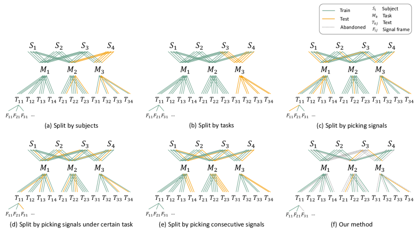
Figure 2: Different cognitive dataset splitting methods.

2 Related Work

Cognitive Signal Cognitive signals can be classified into three categories: invasive, partially invasive, and non-invasive according to how close electrodes get to brain tissue. Due to the high cost and complexity of invasive and partially invasive methods, it’s hard to apply them in building generic and practical BCIs. In this paper, we mainly focus on non-invasive signals EEG and fMRI. EEG signal is electrogram of the spontaneous electrical activity of the brain. Its frequencies usually range from 1 to 30 Hz, divided into several groups like alpha (4-13 Hz), beta (13-30 Hz), delta (0.5-4 Hz), theta (4-7 Hz). EEG is of high temporal resolution and relatively tolerant of subject movement, but its spatial resolution is low and it can’t display active areas of the brain directly. fMRI measures brain activity by detecting changes of blood flow. Blood flow of a specific region increases when this brain area is in use. The spatial resolution of fMRI is measured by the size of voxel, which is a three-dimensional rectangular cuboid ranging from 3mm to 5mm (Vouloumanos et al., 2001; Noppeney and Price, 2004). Unlike EEG which samples brain signals continuously, fMRI samples according to the smallest time period named TR, usually at second level.

Brain-to-text Decoding Previous research on brain-to-text decoding (Herff et al., 2015; Anumanchipalli et al., 2019; Zou et al., 2021; Moses et al., 2021; Défossez et al., 2023) mainly focused on word-level decoding in a restricted vocabulary with hundreds of words (Panachakel and Ramakrishnan, 2021). These models typically apply recurrent neural network or long short-term memory (Hochreiter and Schmidhuber, 1997) network to build mapping between cognitive signals and words in vocabulary. Despite relatively good accuracy, these methods fail to generalize to unseen words. Some progress (Sun et al., 2019) has been made by expanding word-level decoding to sentence-level through encoder-decoder framework, or use less noisy ECoG data (Burle et al., 2015; Anumanchipalli et al., 2019). However, these models struggle to generate accurate and fluent sentences limited by decoder ability. Wang and Ji (2022) introduced the first open vocabulary EEG-to-text decoding model by leveraging the power of pre-trained language models. Xi et al. (2023) improved the model design and proposed a unified framework for decoding both fMRI and EEG signals.

3 Methodology

In this section, we will first introduce the definition of decoding cognitive signals to text and the general description of dataset format. Then we systematically analyze current dataset splitting methods and point out that all existing methods suffer from two kinds of data contamination: cognitive signal leakage and text stimuli leakage. Finally, a new dataset splitting method is proposed to avoid the above-mentioned two kinds of data contamination.

3.1 Task Definition

Given the cognitive signal $F_{ij}$ stimulated by $i$-th subject $S_{i}$ hearing or reading certain text $T_{j}$, brain-to-text decoding aims to decode $F_{ij}$ back to text $T_{j}^{\prime}$ and make $T_{j}^{\prime}$ as similar as possible to $T_{j}$. The composition of $F_{ij}$ and $T_{j}$ is different as to fMRI and EEG. The former samples brain information discretely with a fixed time interval TR, while the latter samples continuously. To fMRI, $L$ consistent sentence segments $s_{j}$ with corresponding fMRI frames $f_{ij}$ are concatenated to form a sample pair $\left\langle F_{ij},T_{j}\right\rangle$. Here $T_{j}=concat(s_{j},s_{j+1},\ldots,s_{j+L-1})$ and $F_{ij}=concat(f_{ij},f_{i,j+1},\ldots,f_{i,j+L-1})$. To EEG, since signals corresponding to a complete sentence are available, we bond sentence (aka text stimuli) $T_{j}$ and EEG signal $F_{ij}$ together to form a sample pair $\left\langle F_{ij},T_{j}\right\rangle$. Under most circumstances, each sentence $T_{j}$ belongs to one certain task $M_{k}$. So the signal-sentence pair $\left\langle F_{ij},T_{j}\right\rangle$ can be further split into $\left\langle F_{ij},M_{k}\right\rangle$ and $\left\langle M_{k},T_{kj}\right\rangle$.

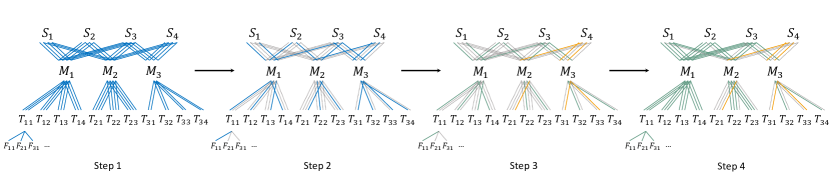
Figure 3: The process of our proposed dataset splitting method.

In brain-to-text decoding, the ultimate goal of trained BCI models is to generalize to unseen subjects with unseen text stimuli (Huang et al., 2010; Handiru and Prasad, 2016; Gao et al., 2021). As a result, if cognitive signal $F_{ij}$ appears in test set $S_{test}$, then any subject $i$’s signal $F_{i}$ should not appear in training set $S_{train}$. Similarly, text stimuli $T_{kj}$ in $S_{test}$ should not appear in $S_{train}$. So the dataset splitting rules can be formally defined as:

$$S_{train}=\{\left\langle F_{ij},T_{kj}\right\rangle|F_{i},T_{kj}\notin S_{val},S_{test}\}$$ (1)

$$S_{val}=\{\left\langle F_{ij},T_{kj}\right\rangle|F_{i},T_{kj}\notin S_{train},S_{test}\}$$ (2)

$$S_{test}=\{\left\langle F_{ij},T_{kj}\right\rangle|F_{i},T_{kj}\notin S_{train},S_{val}\}$$ (3)

3.2 Dataset Splitting Methods

Current dataset splitting methods can be summarized as five categories according to classifying objectives $S_{i},M_{k},T_{kj},F_{ij}$. More specifically, the five dataset splitting methods are characterised as (1) split by subjects, (2) split by tasks, (3) split by randomly picking signal frames, (4) split by randomly picking signal frames under certain task, (5) split by randomly picking consecutive signal frames under certain task, corresponding to image (a), (b), (c), (d), (e) in Figure 2. Figure 2 vividly displays the differences between current dataset splitting methods. For simplicity of expression, we choose four subjects with three tasks each containing four, three, four sentences. The line connecting two symbols indicates they are related to one sample. Take path $S_{1},M_{1},T_{11},F_{11}$ for example, it’s one sample where subject $S_{1}$ listens to text stimuli $T_{11}$ belonging to task $M_{1}$ and $S_{1}$’s corresponding brain signal is recorded as $F_{11}$. Some symbols are connected with several lines. For example, the four lines between $S_{1}$ and $M_{1}$ correspond to $\left\langle M_{1},T_{11}\right\rangle$, $\left\langle M_{1},T_{12}\right\rangle$, $\left\langle M_{1},T_{13}\right\rangle$, $\left\langle M_{1},T_{14}\right\rangle$ counting from left to right. Similarly, the three lines between $M_{1}$ and $T_{11}$ correspond to $\left\langle S_{1},M_{1}\right\rangle$, $\left\langle S_{2},M_{1}\right\rangle$, $\left\langle S_{3},M_{1}\right\rangle$ respectively. The same rules can be extended to other lines and symbols. The green lines and orange lines stand for training samples and testing samples. The grey dotted line means the sample is abandoned, which will be introduced in our dataset splitting method. As the splitting of validation set is similar to test set, we only consider training set and test set in this section.

We will use method (a), (b), (c), (d), (e) to represent five current dataset splitting methods in the rest of the paper. Method (a) splits the dataset according to subjects, which can be described as

$$S_{train}=\{\left\langle F_{ij},T_{kj}\right\rangle|S_{i}\notin S_{val},S_{test}\}$$ (4)

for training set. Method (b) splits the dataset according to tasks, which can be described as

$$S_{train}=\{\left\langle F_{ij},T_{kj}\right\rangle|M_{k}\notin S_{val},S_{test}\}$$ (5)

for training set. Method (c), (d), and (e) all split the dataset according to cognitive signal frames

$$S_{train}=\{\left\langle F_{ij},T_{kj}\right\rangle|F_{ij}\notin S_{val},S_{test}\}.$$ (6)

However, there are slight differences between these methods. Method (c) views all the cognitive signal frames in dataset as a whole and splits according to the default proportion (e.g. 8:1:1). Method (d) views signal frames under certain task $M_{k}$ as a whole and splits proportionally, and then union all training sets under different tasks to form a complete set for training. Method (e) is similar to method (d). They both first split training, validation, and test set under certain task proportionally and then union them. The difference lies in that method (d) randomly picks signal frames while method (e) picks consecutive signal frames.

Type	Method	Narratives / ZuCo				Average
		seed$1$	seed$2$	seed$3$	seed$4$
CSLR$(\%)$	(a)	0.00 / 0.00	0.00 / 0.00	0.00 / 0.00	0.00 / 0.00	0.00 / 0.00
	(b)	6.73 / -	6.32 / -	7.7 / -	17.93 / -	9.67 / -
	(c)	12.55 / 12.52	12.52 / 12.55	12.48 / 12.48	12.44 /12.46	12.50 / 12.50
	(d)	12.81 / 12.60	12.8 / 12.58	12.78 / 12.56	12.79 / 12.61	12.795 / 12.59
	(e)	12.28 / -	12.27 / -	12.26 / -	12.27 / -	12.27 / -
	(f)	0.00 / 0.00	0.00 / 0.00	0.00 / 0.00	0.00 / 0.00	0.00 / 0.00
TSLR$(\%)$	(a)	100.00 / 23.43	100.00 / 20.25	100.00 / 23.38	100.00 / 22.95	100.00 / 22.50
	(b)	0.00 / -	0.00 / -	0.00 / -	0.00 / -	0.00 / -
	(c)	100.00 / 13.21	100.00 / 13.06	100.00 / 12.91	100.00 / 13.1	100.00 / 13.07
	(d)	99.93 / 0.00	99.81 / 0.00	99.54 / 0.00	99.99 / 0.00	99.82 / 0.00
	(e)	9.19 / -	9.31 / -	9.36 / -	9.29 / -	9.29 / -
	(f)	0.00 / 0.00	0.00 / 0.00	0.00 / 0.00	0.00 / 0.00	0.00 / 0.00

Table 1: Results of Cognitive Signal Leakage Rate (CSLR) and Text Stimuli Leakage Rate (TSLR).

The goal of brain-to-text decoding models is to generalize to unseen subjects with unseen text stimuli, which means both subject’s brain information and received text stimuli are new to the trained model. In this sense, we define two kinds of data contamination: cognitive signal leakage and text stimuli leakage. The data contamination situation of different methods is reflected in Figure 2. If lines associated with $S_{i}$ or $T_{kj}$ are of different colours, data in test set leaks into training set. Lines between $S_{i}$ and $M_{k}$ indicate cognitive signal leakage situation and lines between $T_{kj}$ and $M_{k}$ indicate text stimuli leakage situation. Remind the composition of samples differs as to fMRI signal and EEG signal, so the dataset splitting methods are different for two cognitive signals too. Since fMRI signals need to be sampled continuously with a certain length $L$, the path of a sample shown in Figure 2 is actually the first part of one fMRI sample, with $L-1$ continuous part following. In this sense, for EEG cognitive signal leakage doesn’t exist in method (a), but method (a) suffers from text stimuli leakage. The situation of method (b) is opposite to that of method (a), where there’s no text stimuli leakage but cognitive signal leakage. Method (c) and method (d) are similar. They suffer from both cognitive signal leakage and text stimuli leakage. Method (e) is in the same situation as method (b). For fMRI, method (c), (d), and (e) which seem the same for EEG are actually different splitting ways. The situation of data contamination for different methods is similar to EEG, except for method (e) there still exists slight text stimuli leakage in the overlap between training samples and test samples.

3.3 Our Method

To eliminate data contamination from both cognitive signal leakage and text stimuli leakage, we split the dataset by $\left\langle S_{i},T_{j}\right\rangle$ pairs as shown in (f) of Figure 2. Since EEG and fMRI are different in the composition of dataset, we treat them separately and propose two dataset splitting methods. As to EEG dataset where $F_{ij}$ and $T_{j}$ form a sample, we consider a bipartite graph $\mathcal{G}_{1}=(\mathcal{U},\mathcal{V},\mathcal{E})$ where $\mathcal{U}=\{S_{i}\}_{i=1}^{N}$, $\mathcal{V}=\{T_{j}\}_{j=1}^{M}$. $\mathcal{E}$ is the edge between node in $\mathcal{U}$ and node in $\mathcal{V}$, indicating $\left\langle S_{i},T_{j}\right\rangle$ pair in the dataset. $N$ is the total number of subjects and $M$ is the total number of unique text stimuli. We assert $M>N$, so $e=(u,v)\in\mathcal{E}$ exists for every $v\in\mathcal{V}$, as each text stimuli is listened or read by at least one subject. As shown in step 2 of Figure 3, first we pick one edge for each node $v\in\mathcal{V}$ and build a new bipartite graph $\mathcal{G}_{2}=(\mathcal{U},\mathcal{V},\mathcal{E}^{\prime})$. Then we split graph $\mathcal{G}_{2}$ by subject $\mathcal{U}$ with the given splitting ratio and form three disjoint graphs $\mathcal{G}_{train},\mathcal{G}_{val},\mathcal{G}_{test}$. In step 4, some edges satisfying zero data contamination condition are not included in the graph. We add these edges to corresponding graphs, extending each graph $\mathcal{G}_{train},\mathcal{G}_{val},\mathcal{G}_{test}$ to its maximally scalable state and finishing the dataset splitting process.

$F_{ij}=concat(f_{ij},f_{i,j+1},\ldots,f_{i,j+L-1})$ and $T_{j}=concat(s_{j},s_{j+1},\ldots,s_{j+L-1})$ form a sample pair in fMRI dataset. If we follow the same process as EEG, text stimuli leakage will occur in the overlapping part of two samples, when one sample is assigned to training set and the other is assigned to validation or test set. We propose a simple solution that achieves the balance between abandoning as little data as possible and ensuring zero data contamination. Instead of $\left\langle S_{i},T_{j}\right\rangle$ pair, we consider $\left\langle S_{i},M_{k}\right\rangle$ pair and apply the above-mentioned algorithm. More details and pseudo-code are available in Appendix B.

Model	Epoch+lr+Method	BLEU-N ($\%$)				ROUGE-1 ($\%$)
		$N=1$	$N=2$	$N=3$	$N=4$	$F$	$P$	$R$
UniCoRN	10+1e-3+(a)	49.56	30.49	21.07	15.49	44.83	50.41	40.65
	10+1e-3+(b)	26.37	7.50	2.48	0.99	22.28	25.99	19.62
	10+1e-3+(c)	50.24	30.83	21.23	15.60	44.68	49.44	41.01
	10+1e-3+(d)	49.63	30.29	20.85	15.32	45.06	50.47	41.03
	10+1e-3+(e)	28.94	9.39	4.07	1.53	21.68	24.64	19.49
UniCoRN∗	20+1e-4+(a)	50.19	34.25	25.98	21.00	46.59	50.36	43.62
	30+1e-4+(a)	55.46	40.99	32.85	27.56	52.08	55.02	49.68
	20+1e-4+(b)	25.91	8.80	3.84	1.66	20.65	27.74	16.57
	30+1e-4+(b)	25.91	8.80	3.84	1.66	20.65	27.74	16.57
	20+1e-4+(c)	72.44	60.84	53.35	47.88	70.52	74.10	67.53
	30+1e-4+(c)	72.82	61.42	53.95	48.44	71.24	74.41	68.57
	20+1e-4+(d)	65.31	51.02	42.54	36.72	62.76	67.09	59.29
	30+1e-4+(d)	66.56	53.00	44.75	39.02	63.89	67.51	60.95
	20+1e-4+(e)	32.15	12.34	5.57	2.45	24.28	30.43	20.35
	30+1e-4+(e)	32.15	12.34	5.57	2.45	24.28	30.43	20.35

Table 2: Generation quality of UniCoRN model for fMRI under different training settings. Here UniCoRN^∗ indicates the encoder of UniCoRN is randomly initialized instead of pre-trained through signal reconstruction task.

4 Experiments and Analysis

We test state-of-the-art brain-to-text decoding models on two popular cognitive datasets. Comprehensive experiments are conducted to prove the existence of the following phenomena: (1) Cognitive signals and text stimuli in test set leak into training set in all current dataset splitting methods. (2) The model’s generalization ability, particularly that of the auto-regressive decoder, has been overestimated due to data contamination. Because the number of tasks in EEG dataset is too small and method (e) makes no difference to EEG as method (d), we only consider method (a), (c), (d).

4.1 Datasets

We apply the "Narratives" (Nastase et al., 2021) dataset for fMRI-to-text decoding and the ZuCo (Hollenstein et al., 2018) dataset for EEG-to-text decoding in experiments. The "Narratives" dataset contains fMRI data from 345 subjects listening to 27 diverse stories. Since the data collection process involves different machines, we only consider fMRI data with $64\times 64\times 27$ voxels. The ZuCo dataset includes 12 healthy adult native English speakers reading English text for 4 to 6 hours. It contains simultaneous EEG and Eye-tracking data. The reading tasks include Normal Reading (NR) and Task-specific Reading (TSR) extracted from movie views and Wikipedia. Both datasets are split into training, validation, and test set with a ratio of 80$\%$, 10$\%$, 10$\%$ in all experiments.

4.2 Implementation

We follow the same settings of UniCoRN (Xi et al., 2023) and EEG2Text (Wang and Ji, 2022), except the datasets are split to the ratio of 8:1:1 for fair comparison. All experiments are conducted on NVIDIA A100-SXM4-40GB GPUs. More details are shown in Appendix A.

Model	Epoch+lr+Method	BLEU-N ($\%$)				ROUGE-1 ($\%$)
		$N=1$	$N=2$	$N=3$	$N=4$	$F$	$P$	$R$
UniCoRN	50+1e-4+(a)	58.09	49.23	43.23	38.43	63.88	61.12	67.50
	80+1e-4+(a)	60.88	50.52	43.42	37.84	65.17	61.16	70.72
	50+1e-4+(c)	52.30	42.89	36.80	32.17	57.39	51.09	67.29
	80+1e-4+(c)	60.78	55.92	53.18	51.10	84.64	63.16	71.50
	50+1e-4+(d)	22.90	7.36	2.71	0.95	17.73	19.90	17.33
	80+1e-4+(d)	22.90	7.36	2.71	0.95	17.73	19.90	17.33
EEG2Text	50+1e-4+(a)	51.22	33.83	22.99	16.05	46.40	46.85	46.58
	80+1e-4+(a)	63.32	52.52	45.19	39.50	65.96	64.74	68.01
	50+1e-4+(c)	53.83	38.99	29.57	23.01	53.64	54.19	53.56
	80+1e-4+(c)	65.42	57.56	52.56	48.60	73.00	69.99	77.01
	50+1e-4+(d)	23.92	8.16	3.21	1.20	20.78	19.96	23.89
	80+1e-4+(d)	23.92	8.16	3.21	1.20	20.78	19.96	23.89

Table 3: Generation quality of UniCoRN and EEG2Text model for EEG under different training settings.

4.3 Data Contamination

We have analyzed two kinds of data contamination, cognitive signal leakage and text stimuli leakage in Methodology section. In this part, we will quantify data contamination situation through experiments.

To better illustrate the extent of data contamination across different dataset splitting methods, we design two novel evaluation metrics named Cognitive Signal Leakage Rate (CSLR) and Text Stimuli Leakage Rate (TSLR) for detecting cognitive signal leakage and text stimuli leakage. Note that the situation for validation set is similar as test set, we only consider test set in experiments. CSLR indicates the average percentage of each subject’s cognitive signals in test set appearing in training set, which could be formulated as

$$\frac{1}{N}\sum_{i=1}^{N}\min(1,\frac{|\{F_{ij}|F_{ij}\in S_{test}\cap S_{train}\}|}{|\{F_{ij}|F_{ij}\in S_{train}\}|})$$ (7)

where $N$ stands for the total number of subjects in test set. $|\cdot|$ stands for the cardinality of a set. Function $\min(\cdot,\cdot)$ is applied to make sure for each subject the data leakage rate is less than 1.

The definition of TSLR is somewhat different for EEG signal and fMRI signal. As to EEG signal where cognitive signals are sampled continuously, it’s easy to match certain sentence stimuli with corresponding signals. Its TSLR is similar to CSLR, which indicates the average percentage of certain text in test set appearing in training set. TSLR for EEG data can be calculated through

$$\frac{1}{M}\sum_{j=1}^{M}\min(1,\frac{|\{T_{ij}|T_{ij}\in S_{test}\cap S_{train}\}|}{|\{T_{ij}|T_{ij}\in S_{train}\}|})$$ (8)

where $M$ stands for the total number of unique text periods in test set and $T_{ij}$ stands for $j$-th period of text stimuli received by $i$-th subject.

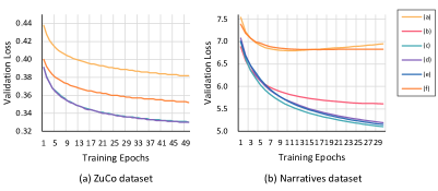
Figure 4: Validation loss of encoder under different dataset splitting methods in two datasets.

The fMRI signal is sampled discretely with a deterministic interval TR, making it hard to acquire signals corresponding to sentences. Previous methods instead concatenated continuous fMRI frames of certain length with their corresponding sentence segments as training samples. As a result, we consider the average percentage of the same sentence segments in test set appearing in training set as TSLR of fMRI signal. It can be formulated as

$$\frac{1}{M}\sum_{j=1}^{M}\tau\frac{|\{T_{ij}|T_{ij}\in S_{test}\cap S_{train}\}|}{|S_{test}|\times L}$$ (9)

where $\tau=0$ if $\{T_{ij}|T_{ij}\in S_{test}\cap S_{train}\}=\emptyset$ else

$$\tau=\min(1,\frac{|\{T_{ij}|T_{ij}\in S_{train}\}|}{|\{T_{ij}|T_{ij}\in S_{test}\cap S_{train}\}|}).$$ (10)

We test current dataset splitting methods and our method on fMRI dataset Narratives and EEG dataset ZuCo. Considering the influence of randomness in splitting, we select four seeds for experiments. The results are shown in Table 1 and are consistent with theoretical analysis. For fMRI, current methods apart from method (a) suffer from cognitive signal leakage, while method (a) has serious text stimuli leakage. Method (b) gets no text stimuli leakage but has slight cognitive signal leakage. The situation for EEG is similar to that of fMRI. Apart from our proposed method (f), there is no way to achieve zero cognitive signal leakage and text stimuli leakage at the same time.

Dataset	Model	BLEU-N ($\%$)				ROUGE-1 ($\%$)
		$N=1$	$N=2$	$N=3$	$N=4$	$F$	$P$	$R$
Narratives	UniCoRN	22.83	5.69	1.43	0.48	15.55	24.80	19.04
ZuCo	UniCoRN	23.32	7.78	3.01	1.09	18.47	20.00	17.92
	EEG2Text	24.49	7.49	2.28	0.62	23.98	23.95	25.74

Table 4: A fair benchmark for evaluating brain-to-text decoding.

4.4 Overestimated Performance

Cognitive signal leakage and text stimuli leakage affect models from encoder side and decoder side.

4.4.1 Encoder

As shown in Figure 1, encoder in current models is trained in two different ways: either jointly trained with decoder or solely trained through a reconstruction task. In the former end-to-end training scenario, it’s hard to evaluate encoder performance separately. So we mainly focus on the latter, in which case the encoder is trained through an encoder-decoder framework to reconstruct input cognitive signals. The decoder here doesn’t refer to the decoder for text generation. It’s similar to the structure of the encoder and will be abandoned once the encoder is trained. Although a proper evaluation index of the encoder’s representation ability is missing, validation loss is used to measure the influence of data contamination.

We test different splitting methods on two cognitive datasets. The validation loss of encoder is shown in Figure 4. For fMRI, influenced by leakage of cognitive signals, the validation loss of method (b), (c), (d), (e) keeps dropping even with long training epochs. The encoder is actually overfitting and degrading. For method (a) and (f) without cognitive signal leakage, the validation loss quickly rises after reaching the lowest point with a few epochs, satisfying the basic rule of machine learning. For EEG, we find validation loss keeps dropping for all methods even with very long training epochs, regardless of cognitive signal leakage or not. We think the poor spatial resolution of EEG signal might lead to this phenomenon.

4.4.2 Decoder

All state-of-the-art models choose pre-trained language model BART (Lewis et al., 2020) as decoder. On one hand, the powerful auto-regressive decoder is able to achieve fluent sentence-level open vocabulary text generation. On the other hand, if data contamination occurs, due to the feature of auto-regressive generation, the decoder will generate memorized text given the first few words, which is obviously an act of cheating.

The influence of text stimuli leakage on decoder is detected through BLEU scores (Papineni et al., 2002) and ROUGE-1 scores (Lin, 2004), which measure text similarity between generated text and ground truth. If evaluation indicators keep improving as training epochs increase, we believe part of the test set is leaked into training set and the model is overfitting. For fMRI signal, we test five current dataset splitting methods under different training settings. As shown in Table 2, we test two kinds of UniCoRN models. One is UniCoRN with finely tuned hyper-parameters claimed in the original paper, and the other is UniCoRN^∗ with a randomly initialized encoder. Empirically, the former will perform much better than the latter. However, in method (a), (c), (d), due to text stimuli leakage, if we reduce the learning rate and extend training epochs, UniCoRN^∗ performs much better than UniCoRN and its performance keeps rising with longer training epochs. As to method (b) and (e) with no text stimuli leakage, changing training epochs or learning rates makes no obvious difference to model performance. For EEG signal, the conclusion is similar as shown in Table 3. For method (a) and (c) with text stimuli leakage, model performance keeps rising with longer training epochs. For method (d) without text stimuli leakage, both models reach optimal performance after the first few rounds of training epochs.

4.5 Fair Benchmark

We evaluate current SOTA models for brain-to-text decoding under our dataset splitting method and release a fair benchmark. UniCoRN is tested for both fMRI and EEG decoding, EEG2Text model is tested for EEG decoding. The results are listed in Table 4. For EEG dataset, UniCoRN achieves higher results in BLEU-2,3,4 while EEG2Text is better in BLEU-1 and ROUGE-1.

5 Conclusion

In this paper, we explore a controversial topic: Due to the complexity of cognitive datasets, no consensus has been reached on how to split the dataset for training, validating, and testing in brain-to-text decoding. We analyze current dataset splitting methods and find serious data contamination largely exaggerates model performance and leads to poor generalization. Sufficient experiments and analysis are conducted to prove the existence of the above phenomena. Moreover, we propose a new dataset splitting method which can avoid both cognitive signal and text stimuli leakage to fix this problem. Current state-of-the-art models are reevaluated under this setting and a fair benchmark is released for further research in the domain.

Limitations

The "Narratives" dataset and the ZuCo dataset provide researchers with precise cognitive signal resources stimulated by text or voice. However, in brain-to-text decoding task, both subject’s cognitive signals and text stimuli in validation and test set need to be invisible to training set, which makes splitting these public datasets difficult. Our proposed dataset splitting method meets the above requirements at the expense of discarding some data in the dataset. We recommend future datasets in this domain follow these guidelines. The division of the training set, validation set, and test set should be provided when the dataset is released. Besides, we suggest hiring new subjects with unique stimuli for validation set and test set, which is good for testing the generalization ability of models without loss of data (Tang et al., 2023). What’s more, we find existing models rely more on the strong auto-regressive decoder to achieve good generation quality. The encoder is of limited use in all SOTA models, which might become a research point in the future.

Ethics Statement

In this paper, we introduce a new dataset splitting method to avoid data contamination for decoding cognitive signals to text task. Experiments are conducted on public accessible cognitive datasets Narratives and ZuCo1.0 with the authorization from their respective maintainers. Both datasets have been de-identified by dataset providers and used for researches only.

Appendix A Implementation Details

More details in experiments are supplemented in this section. We perform the same filtering steps to Narratives dataset as UniCoRN paper (Xi et al., 2023) and the same filtering steps to ZuCo1.0 as EEG2Text paper (Wang and Ji, 2022). In CSLR and TSLR calculation, the number of four different seeds are set as $1,2,3,4$ respectively. In signal reconstruction task for encoder of UniCoRN, the batch size of EEG and fMRI data is 512 and 320 respectively. The learning rate is set as 1e-4 and 1e-3 separately as the author claimed in the original paper. In the fair benchmark, for fMRI data, encoder of UniCoRN is trained through 1e-4 learning rate and decaying to 1e-6 finally for 30 training epochs. Decoder is trained through 1e-4 learning rate and decaying to 1e-6 finally for 10 training epochs with 90 batch size. Sample length $L$ is set as 10 for all experiments related to fMRI. For EEG data, EEG2Text model is trained with 1e-6 learning rate for 80 epochs. UniCoRN model is trained with the same settings as fMRI data.

Appendix B Our Dataset Splitting Method

In this part, we release the pseudo-code of two dataset splitting methods for EEG and fMRI signal. As shown in Figure 3, our proposed dataset splitting method consists of four steps. The blue lines stand for the situation of original dataset. The main difference between two methods lies in the how $\mathcal{G}_{2}$ is generated. We always choose the side with fewer nodes in bipartite graph $\mathcal{G}_{1}$ to perform $\mathcal{G}_{2}$ generation. For example, in Algorithm 1 where we assert $|\mathcal{U}|<|\mathcal{V}|$, the adjacency matrix is initialized as $M\times N$. In Algorithm 2 where $|\mathcal{V}|<|\mathcal{U}|$, the adjacency matrix is initialized as $N\times K$. All hypotheses are based on analysis of cognitive datasets.

One more thing to notice is that in Line 14 of both pseudo-code, the loop indicates extending training set, validation set, and test set respectively. So the names of variable should be alternated in the repeat loop and the displayed part in pseudo-cod is a case example of extending training set. We write it in this way for simplicity of expression.

1 Initialize: Bipartite graph $\mathcal{G}_{1}=(\mathcal{U},\mathcal{V},\mathcal{E})$, $\mathcal{G}_{2}=(\mathcal{U},\mathcal{V},\mathcal{E}^{\prime})$ where $\mathcal{U}=\{S_{i}\}_{i=1}^{N}$ and $\mathcal{V}=\{T_{j}\}_{j=1}^{M}$, Adjacency matrix $A_{1}$ of $\mathcal{G}_{1}$ where $A_{1}[i][j]=1$ if node $i$ and node $j$ is connected else $A_{1}[i][j]=0$, Adjacency matrix $A_{2}$ of $\mathcal{G}_{2}$ where $A_{2}[i][j]=0$, Array $C$ where $len(C)=len(\mathcal{U})$ and $C[i]=0$;

2 for $u\leftarrow U_{1}$ to $U_{N}$ do

3       $C_{copy}\leftarrow C$;

4       for $v\leftarrow A_{1}[u][0]$ to $A_{1}[u][M]$ do

5             if $v=0$ then

6                  $C_{copy}[v.index]\leftarrow\infty$;

7            

8      Minimum $=\min(C_{copy})$;

9       $A_{2}[u][$Minimum$.index]\leftarrow 1$;

10       $C[$Minimum$.index]\leftarrow C[$Minimum$.index]+1$; // Make degree of nodes balanced 

11Split by subjects $\mathcal{U}$ according to default ratio;

12 $\mathcal{G}_{2}=\mathcal{G}_{train}\cup\mathcal{G}_{val}\cup\mathcal{G}_{test},\,\mathcal{U}_{train}\cap\mathcal{U}_{val}\cap\mathcal{U}_{test}=\emptyset,\,\mathcal{V}_{train}\cap\mathcal{V}_{val}\cap\mathcal{V}_{test}=\emptyset$;

13 repeat // To three sets respectively, below is for training set

14       for $u$ in $\mathcal{U}$  do

15             for $v$ in $\mathcal{V}$ do

16                   if $e=(u,v)\in\mathcal{E}$ and $e=(u,v)\notin\mathcal{E}^{\prime}_{train}$ and $u\notin\mathcal{U}_{val}\cup\mathcal{U}_{test}$ then

17                        $\mathcal{E}_{train}^{\prime}\leftarrow\mathcal{E}_{train}^{\prime}\cup\{e\}$;

18                  

19            

20      

21until $\mathcal{G}_{train},\mathcal{G}_{val},\mathcal{G}_{test}$ are all extended;

22return $\mathcal{G}_{train},\mathcal{G}_{val},\mathcal{G}_{test}$;

Algorithm 1 Dataset splitting method for EEG signal

23 Initialize: Bipartite graph $\mathcal{G}_{1}=(\mathcal{U},\mathcal{V},\mathcal{E})$, $\mathcal{G}_{2}=(\mathcal{U},\mathcal{V},\mathcal{E}^{\prime})$ where $\mathcal{U}=\{S_{i}\}_{i=1}^{N}$, $\mathcal{V}=\{M_{k}\}_{k=1}^{K}$, Adjacency matrix $A_{1}$ of $\mathcal{G}_{1}$ where $A_{1}[i][j]=1$ if node $i$ and node $j$ is connected else $A_{1}[i][j]=0$, Adjacency matrix $A_{2}$ of $\mathcal{G}_{2}$ where $A_{2}[i][j]=0$, Array $C$ where $len(C)=len(\mathcal{V})$ and $C[i]=0$;

24 for $v\leftarrow V_{1}$ to $V_{K}$ do

25       $C_{copy}\leftarrow C$;

26       for $u\leftarrow A_{1}[v][0]$ to $A_{1}[v][K]$ do

27             if $u=0$ then

28                  $C_{copy}[u.index]\leftarrow\infty$;

29            

30      Minimum $=\min(C_{copy})$;

31       $A_{2}[v][$Minimum$.index]\leftarrow 1$;

32       $C[$Minimum$.index]\leftarrow C[$Minimum$.index]+1$; // Make degree of nodes balanced 

33Split by tasks $\mathcal{V}$ according to default ratio;

34 $\mathcal{G}_{2}=\mathcal{G}_{train}\cup\mathcal{G}_{val}\cup\mathcal{G}_{test},\,\mathcal{U}_{train}\cap\mathcal{U}_{val}\cap\mathcal{U}_{test}=\emptyset,\,\mathcal{V}_{train}\cap\mathcal{V}_{val}\cap\mathcal{V}_{test}=\emptyset$;

35 repeat // To three sets respectively, below is for training set

36       for $v$ in $\mathcal{V}$  do

37             for $u$ in $\mathcal{U}$ do

38                   if $e=(u,v)\in\mathcal{E}$ and $e=(u,v)\notin\mathcal{E}^{\prime}_{train}$ and $v\notin\mathcal{V}_{val}\cup\mathcal{V}_{test}$ then

39                        $\mathcal{E}_{train}^{\prime}\leftarrow\mathcal{E}_{train}^{\prime}\cup\{e\}$;

40                  

41            

42      

43until $\mathcal{G}_{train},\mathcal{G}_{val},\mathcal{G}_{test}$ are all extended;

44return $\mathcal{G}_{train},\mathcal{G}_{val},\mathcal{G}_{test}$;

Algorithm 2 Dataset splitting method for fMRI signal

References

- Anumanchipalli et al. (2019) Gopala K Anumanchipalli, Josh Chartier, and Edward F Chang. 2019. Speech synthesis from neural decoding of spoken sentences. Nature, 568(7753):493–498.
- Bahdanau et al. (2015) Dzmitry Bahdanau, Kyunghyun Cho, and Yoshua Bengio. 2015. Neural machine translation by jointly learning to align and translate. In 3rd International Conference on Learning Representations, ICLR 2015, San Diego, CA, USA, May 7-9, 2015, Conference Track Proceedings.
- Bouton et al. (2016) Chad E Bouton, Ammar Shaikhouni, Nicholas V Annetta, Marcia A Bockbrader, David A Friedenberg, Dylan M Nielson, Gaurav Sharma, Per B Sederberg, Bradley C Glenn, W Jerry Mysiw, et al. 2016. Restoring cortical control of functional movement in a human with quadriplegia. Nature, 533(7602):247–250.
- Burle et al. (2015) Boris Burle, Laure Spieser, Clémence Roger, Laurence Casini, Thierry Hasbroucq, and Franck Vidal. 2015. Spatial and temporal resolutions of eeg: Is it really black and white? a scalp current density view. International Journal of Psychophysiology, 97(3):210–220.
- Défossez et al. (2023) Alexandre Défossez, Charlotte Caucheteux, Jérémy Rapin, Ori Kabeli, and Jean-Rémi King. 2023. Decoding speech perception from non-invasive brain recordings. Nature Machine Intelligence, 5(10):1097–1107.
- Gao et al. (2021) Xiaorong Gao, Yijun Wang, Xiaogang Chen, and Shangkai Gao. 2021. Interface, interaction, and intelligence in generalized brain–computer interfaces. Trends in Cognitive Sciences, 25(8):671–684.
- Handiru and Prasad (2016) Vikram Shenoy Handiru and Vinod A. Prasad. 2016. Optimized bi-objective eeg channel selection and cross-subject generalization with brain–computer interfaces. IEEE Transactions on Human-Machine Systems, 46(6):777–786.
- Herff et al. (2015) Christian Herff, Dominic Heger, Adriana De Pesters, Dominic Telaar, Peter Brunner, Gerwin Schalk, and Tanja Schultz. 2015. Brain-to-text: decoding spoken phrases from phone representations in the brain. Frontiers in neuroscience, 9:217.
- Hochberg et al. (2012) Leigh R Hochberg, Daniel Bacher, Beata Jarosiewicz, Nicolas Y Masse, John D Simeral, Joern Vogel, Sami Haddadin, Jie Liu, Sydney S Cash, Patrick Van Der Smagt, et al. 2012. Reach and grasp by people with tetraplegia using a neurally controlled robotic arm. Nature, 485(7398):372–375.
- Hochreiter and Schmidhuber (1997) Sepp Hochreiter and Jürgen Schmidhuber. 1997. Long short-term memory. Neural Comput., 9(8):1735–1780.
- Hollenstein et al. (2018) Nora Hollenstein, Jonathan Rotsztejn, Marius Troendle, Andreas Pedroni, Ce Zhang, and Nicolas Langer. 2018. Zuco, a simultaneous eeg and eye-tracking resource for natural sentence reading. Scientific data, 5(1):1–13.
- Huang et al. (2010) Gan Huang, Guangquan Liu, Jianjun Meng, Dingguo Zhang, and Xiangyang Zhu. 2010. Model based generalization analysis of common spatial pattern in brain computer interfaces. Cognitive neurodynamics, 4:217–223.
- Lewis et al. (2020) Mike Lewis, Yinhan Liu, Naman Goyal, Marjan Ghazvininejad, Abdelrahman Mohamed, Omer Levy, Veselin Stoyanov, and Luke Zettlemoyer. 2020. BART: denoising sequence-to-sequence pre-training for natural language generation, translation, and comprehension. In Proceedings of the 58th Annual Meeting of the Association for Computational Linguistics, ACL 2020, Online, July 5-10, 2020, pages 7871–7880. Association for Computational Linguistics.
- Lin (2004) Chin-Yew Lin. 2004. Rouge: A package for automatic evaluation of summaries. In Text summarization branches out, pages 74–81.
- Makin et al. (2020) Joseph G Makin, David A Moses, and Edward F Chang. 2020. Machine translation of cortical activity to text with an encoder–decoder framework. Nature neuroscience, 23(4):575–582.
- Moses et al. (2021) David A Moses, Sean L Metzger, Jessie R Liu, Gopala K Anumanchipalli, Joseph G Makin, Pengfei F Sun, Josh Chartier, Maximilian E Dougherty, Patricia M Liu, Gary M Abrams, et al. 2021. Neuroprosthesis for decoding speech in a paralyzed person with anarthria. New England Journal of Medicine, 385(3):217–227.
- Mridha et al. (2021) Muhammad F Mridha, Sujoy Chandra Das, Muhammad Mohsin Kabir, Aklima Akter Lima, Md Rashedul Islam, and Yutaka Watanobe. 2021. Brain-computer interface: Advancement and challenges. Sensors, 21(17):5746.
- Nastase et al. (2021) Samuel A Nastase, Yun-Fei Liu, Hanna Hillman, Asieh Zadbood, Liat Hasenfratz, Neggin Keshavarzian, Janice Chen, Christopher J Honey, Yaara Yeshurun, Mor Regev, et al. 2021. The “narratives” fmri dataset for evaluating models of naturalistic language comprehension. Scientific data, 8(1):250.
- Noppeney and Price (2004) Uta Noppeney and Cathy J Price. 2004. An fmri study of syntactic adaptation. Journal of Cognitive Neuroscience, 16(4):702–713.
- Panachakel and Ramakrishnan (2021) Jerrin Thomas Panachakel and Angarai Ganesan Ramakrishnan. 2021. Decoding covert speech from eeg-a comprehensive review. Frontiers in Neuroscience, 15:392.
- Papineni et al. (2002) Kishore Papineni, Salim Roukos, Todd Ward, and Wei-Jing Zhu. 2002. Bleu: a method for automatic evaluation of machine translation. In Proceedings of the 40th Annual Meeting of the Association for Computational Linguistics, July 6-12, 2002, Philadelphia, PA, USA, pages 311–318. ACL.
- Polikov et al. (2005) Vadim S Polikov, Patrick A Tresco, and William M Reichert. 2005. Response of brain tissue to chronically implanted neural electrodes. Journal of neuroscience methods, 148(1):1–18.
- Sun et al. (2019) Jingyuan Sun, Shaonan Wang, Jiajun Zhang, and Chengqing Zong. 2019. Towards sentence-level brain decoding with distributed representations. In The Thirty-Third AAAI Conference on Artificial Intelligence, AAAI 2019, The Thirty-First Innovative Applications of Artificial Intelligence Conference, IAAI 2019, The Ninth AAAI Symposium on Educational Advances in Artificial Intelligence, EAAI 2019, Honolulu, Hawaii, USA, January 27 - February 1, 2019, pages 7047–7054. AAAI Press.
- Sutskever et al. (2014) Ilya Sutskever, Oriol Vinyals, and Quoc V. Le. 2014. Sequence to sequence learning with neural networks. In Advances in Neural Information Processing Systems 27: Annual Conference on Neural Information Processing Systems 2014, December 8-13 2014, Montreal, Quebec, Canada, pages 3104–3112.
- Tang et al. (2023) Jerry Tang, Amanda LeBel, Shailee Jain, and Alexander G Huth. 2023. Semantic reconstruction of continuous language from non-invasive brain recordings. Nature Neuroscience, pages 1–9.
- Vouloumanos et al. (2001) Athena Vouloumanos, Kent A Kiehl, Janet F Werker, and Peter F Liddle. 2001. Detection of sounds in the auditory stream: event-related fmri evidence for differential activation to speech and nonspeech. Journal of Cognitive Neuroscience, 13(7):994–1005.
- Wang and Ji (2022) Zhenhailong Wang and Heng Ji. 2022. Open vocabulary electroencephalography-to-text decoding and zero-shot sentiment classification. In Thirty-Sixth AAAI Conference on Artificial Intelligence, AAAI 2022, Thirty-Fourth Conference on Innovative Applications of Artificial Intelligence, IAAI 2022, The Twelveth Symposium on Educational Advances in Artificial Intelligence, EAAI 2022 Virtual Event, February 22 - March 1, 2022, pages 5350–5358. AAAI Press.
- Xi et al. (2023) Nuwa Xi, Sendong Zhao, Haochun Wang, Chi Liu, Bing Qin, and Ting Liu. 2023. Unicorn: Unified cognitive signal reconstruction bridging cognitive signals and human language. In Proceedings of the 61st Annual Meeting of the Association for Computational Linguistics (Volume 1: Long Papers), ACL 2023, Toronto, Canada, July 9-14, 2023, pages 13277–13291. Association for Computational Linguistics.
- Zou et al. (2021) Shuxian Zou, Shaonan Wang, Jiajun Zhang, and Chengqing Zong. 2021. Towards brain-to-text generation: Neural decoding with pre-trained encoder-decoder models. In NeurIPS 2021 AI for Science Workshop.