Predict and Interpret Health Risk using EHR through Typical Patients

Abstract

Predicting health risks from electronic health records (EHR) is a topic of recent interest. Deep learning models have achieved success by modeling temporal and feature interaction. However, these methods learn insufficient representations and lead to poor performance when it comes to patients with few visits or sparse records. Inspired by the fact that doctors may compare the patient with typical patients and make decisions from similar cases, we propose a Progressive Prototypical Network (PPN) to select typical patients as prototypes and utilize their information to enhance the representation of the given patient. In particular, a progressive prototype memory and two prototype separation losses are proposed to update prototypes. Besides, a novel integration is introduced for better fusing information from patients and prototypes. Experiments on three real-world datasets demonstrate that our model brings improvement on all metrics. To make our results better understood by physicians, we developed an application at http://ppn.ai-care.top. Our code is released at https://github.com/yzhHoward/PPN.

Index Terms—  Electronic health record, healthcare analysis, prototype learning, interpretability

1 Introduction

As electronic systems widely used in hospitals, electronic health records (EHR) can be used to build models to predict health risks and improve healthcare quality. In recent years, deep learning approaches have achieved early success using EHR data. Most of these works attempt to model temporal information [1, 2, 3], capture feature correlation [2, 4], and find important visits [5, 6, 7].

However, patients with few visits or highly sparse records are common in EHR data. For example, some patients may visit multiple hospitals, resulting in some records being unavailable due to privacy protection [8]; or not testing the same indicators in adjacent visits, resulting in sparse observations. In these cases, traditional representation learning methods may only capture insufficient information and learn low-discriminative representations.

To tackle this problem, we draw inspiration from the routine practices of doctors: When a doctor receives a new patient, the doctor may compare the patient with previous typical cases to understand the health status [9, 10, 11]. So, can we select typical patients and utilize their knowledge to enhance representations of patients? We attempt to build a model to select typical cases as prototypes and facilitate the representations of patients through these cases.

While learning and utilizing typical patients, there are following challenges. One the one hand, the physical status of the patient is complicated. There are many implicit subtypes among patients, and the patients belonging to the same subtype may have different outcomes [12]. Learning prototypes by outcomes like traditional methods [13, 14] ignores the subtypes and introduces bias. Besides, the clustering structure between prototypes and patients is crucial. If only use cluster centroids as prototypes at the beginning of the training, the cluster structure cannot be maintained as model updates. Some prototypes may collapse into a single point while training, thereby losing diversity and confusing doctors. On the other hand, how to use prototypes for prediction is still a challenging problem. Most works [15, 16] perform prediction using similarity or distance between prototypes and input, but these manners omit the original information from input. In health prediction, the information from patients is essential and the similarity alone is insufficient.

In this paper, we introduce prototype learning into EHR analysis on the health risk prediction and propose a Progressive Prototypical Network (PPN). PPN learns patient representation by multi-channel feature extraction, and then enhance it by prototypical feature integration with typical patients for health prediction. In selecting typical patients, PPN selects them as prototypes by novel progressive method and utilze prototype separation losses to promote diversity. PPN is enabled by the following contributions:

• A progressive prototype memory and two prototype separation losses and are proposed to obtain typical patients perceptively while ensuring cluster structure.

• An integration method of prototype features is proposed to compute the similarity between prototypes and patients and then incorporate their information.

• Experiments on three datasets verify the effectiveness of PPN. Especially, PPN performs well on data with high missing rate.

• An interactive application is built to visualize the prediction and interpretation from PPN at http://ppn.ai-care.top.

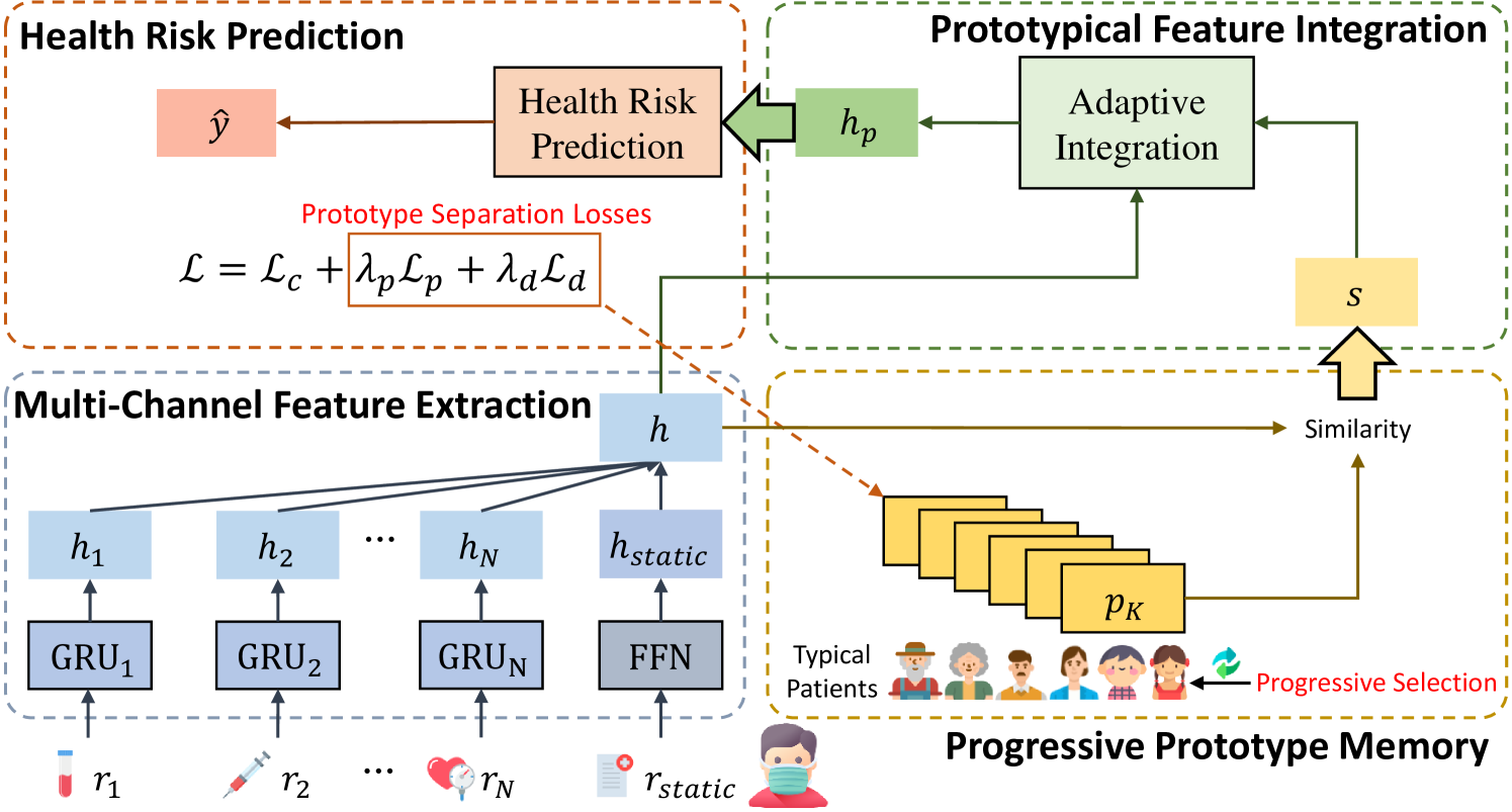
Fig. 1: The framework of PPN. For the EHR of a patient, PPN firstly extracts its health status, computes the similarity coefficient between typical patients, re-weight the health status, and predicts the health risk via the integrated feature

2 Preliminary

Formally, EHR data can be denoted by $(\mathbb{X},\mathbb{Y})$, where $\mathbb{X}\subseteq\mathbb{R}^{T\times N}\cup\mathbb{R}^{M}$ is the input space and $\mathbb{Y}=\{0,1\}$ is the output space. The EHR records $x\in\mathbb{X}$ of a patient is defined as: given a series of $N$-dimensional laboratory tests and dynamic diagnoses, then the record of $n$-th indicators can be represented by $r_{n}$. For different patients, the lengths of series can be different. Additionally, patients have $M$-dimensional demographic data and static diagnoses formulated as $r_{static}$. The health risk prediction problem is to predict whether death risk events occur in the specified time window.

3 Methodology

3.1 Overview

As depicted in Figure 1, PPN can be divided into four parts: multi-channel feature extraction module, progressive prototype memory, prototypical feature integration, and health risk prediction. In the following, each module will be described in detail.

3.2 Multi-Channel Feature Extraction

This module is developed to extract information from the input longitudinal patient matrix and static data to obtain the latent health status representations inspired by ConCare [2]. By embed each feature separately, the model can better model the changing pattern of each indicator.

Specifically, given a sequence of medical records along with a patient, the health status representation of each indicator $h_{n}=\mathrm{GRU}_{n}(r_{n})$, where GRU (Gate Recurrent Unit) is a type of RNN (Recurrent Neural Network). The demographic data embedded by a one-layer feed-forward network (FFN) can be denoted as $h_{static}=\mathrm{FFN}(r_{static})$. Then we concatenate the embedded laboratory tests and demographic data to acquire overall the patient’s health status representation $h=[h_{1},h_{2},...,h_{N},h_{static}],h\in\mathbb{R}^{(N+1)\times H}$, where $H$ denotes the dimension of latent space.

3.3 Progressive Prototype Memory

We select and store typical patients in memory as prototypes. To obtain prototypes that are unrelated to outcomes, we cluster the latent representation $h$ of all patients in the training set to obtain $K$ clusters and take the patients closest to centroids as the prototypes $\mathbb{P}=\{p_{1},p_{2},...,p_{K}\}$, where $p_{j}\in\mathbb{R}^{(N+1)\times H}$. While training, the representation of patients in latent space may shift and decrease the interpretability, so we re-select prototypes at certain epochs progressively to ensure the cluster structure. The clustering algorithm is applied to calculate centroids. The nearest patients to each centroid in the latent space will be new prototypes to replace old prototypes via $p_{j}\leftarrow\mathop{\arg\min}\limits_{i}\|h^{i}-p_{j}\|_{2}$, where $i$ denotes the patient index.

Considering new and old prototypes may represent different subtypes of patients, and replacing them would significantly impact the upper layers, we match the old and new prototypes with the closest overall distance by Jonker-Volgenant algorithm [17]. After selecting prototypes, we freeze embedding layers and the prototype layer and then train the upper network for several epochs to guarantee stability.

3.4 Prototypical Feature Integration

For composing the learned prototypes and health status representation $h$, we create prototypical feature integration that can adaptively combine information of the given patients and prototypes while providing interpretation. Here, the similarity are only adopted to re-weight the health status representation to prevent neglecting of patient information.

In the integration operation, PPN first computes the similarity coefficient $s\in\mathbb{R}^{K}$ between the prototypes and patients via cosine similarity. The coefficient $s$ enhances prototypes with strong correlation and suppresses others.

$$s=\frac{ph}{\|p\|\times\|h\|}$$ (1)

Then we calculate fusing health status $h_{p}$ associated with the coefficient $s$ by

$$h_{p}=h^{\prime\top}s,\quad h^{\prime}=W_{h}h^{\top},$$ (2)

where $W_{h}\in\mathbb{R}^{(N+1)\times K}$.

3.5 Learning Objective

With the integrated health status $h_{p}$, the prediction of health risks can be obtained by

$$\hat{y}=\sigma(f_{out}(h_{p})).$$ (3)

$\sigma$ represents the sigmoid operation, and $f_{out}$ is a one-layer feed-forward network. We use binary cross-entropy loss as the primary learning objective:

$$\mathcal{L}_{c}=-y\mathrm{log}\hat{y}-(1-y)\mathrm{log}(1-\hat{y}).$$ (4)

Though progressive prototype selection update prototypes to ensure cluster structure in certain epochs, is not enough to choose patients from different subtypes. Therefore, we propose prototype separation losses to address this issue. Since the prototypes can be regarded as particular patients, we predict the health risk $y_{j}$ of prototypes $j$ by $p_{j}$ as health status and adopt a separation loss that encourages the prototypes to represent different subtypes of patients:

$$\mathcal{L}_{p}=\sum^{K}_{j}\sum^{K}_{j^{\prime}\neq j}y_{j}\mathrm{log}y^{\prime}_{j}+(1-y_{j})\mathrm{log}(1-y^{\prime}_{j}).$$ (5)

Nevertheless, one critical question that may arise is how to avoid trivial problems of learning the prototypes [18]. For example, some prototypes may collapse into a single point in the latent space, or the prototype coefficients are assigned equally to some prototypes regardless of the input patient. These situations lead to reduced interpretability. [19] proposed two regularization terms to encourage a clustering structure in the latent space by minimizing the squared distance between an encoded sample and its closest prototype. But these terms may cause some samples closer to the cluster they do not belong to. Consequently, we introduce another separation term $\mathcal{L}_{d}$:

$$\mathcal{L}_{d}=\sum^{K}_{j}\sum^{K}_{j^{\prime}\neq j}\mathrm{max}(0,margin-\left\|p_{j}-p_{j^{\prime}}\right\|_{2}).$$ (6)

With loss terms formulated above, we can define the final objective of our model as

$$\mathcal{L}=\mathcal{L}_{c}+\lambda_{p}\mathcal{L}_{p}+\lambda_{d}\mathcal{L}_{d},$$ (7)

where $\lambda_{p}$ and $\lambda_{d}$ are hyper-parameters that control the excitation of prototype separation losses. We use a gradient descent back-propagation algorithm to minimize the loss $\mathcal{L}$ and optimize the parameters.

While training, the representations of prototypes may shift in latent space and they are not readily interpretable. Thus, we design an assigning step during training that assigns $p_{j}$ with the closest patient’ embedding $h^{i}$ of patient $i$ in the training set: $p_{j}\leftarrow\mathop{\arg\min}\limits_{i}\left\|h^{i}-p_{j}\right\|_{2}$.

4 Experiments

In this section, we introduce the datasets and our experimental setup. Then we evaluate our model compared to the state-of-the-art baselines. We conduct analyses showing the effectiveness and interpretability of our proposed modules.

4.1 Datasets

We follow experiment settings from previous works [2, 3, 6, 20]. ESRD, Cardiology, and MIMIC-III datasets are applied for evaluation. The private information are desensitized when preprocessing. ESRD dataset is an end-stage renal disease dataset, collected from diagnosis and treatment data of the peritoneal dialysis department of a hospital. Cardiology dataset [21] is collected from three U.S. ICUs for sepsis prediction. The goal of MIMIC-III dataset [22, 23] is to predict in-hospital mortality based on the first 48 hours of an ICU stay. We illustrate the statistics of these datasets in Table 1.

	ESRD	Cardiology	MIMIC-III
Patient	662	40,336	21,139
Positive outcomes	258	2,932	2,797
Indicators	17	34	17
Total Visits	13,108	1,552,210	1,014,672
Maximum visits	69	336	48
Minimum visits	1	8	48

Table 1: Statistics of datasets

4.2 Experimental Setup and Baselines

The prototypes are initialized by centroids at the beginning of the training. The hidden size $H$ of all modules is 32. We use mini-batch K-Means algorithm while computing centroids to accelerate. To reduce randomness, the old prototypes are regarded as initial centroids in the initialization of K-Means. We try different $K\in\{4,6,8,12,16,20,24,28\}$ on these datasets, and a larger $K$ does not always lead to better results. Finally, when training ESRD dataset, we choose $K=6,\lambda_{p}=0.1$ and $\lambda_{d}=0.05$. For Cardiology dataset, we set $K=16,\lambda_{p}=0.02$ and $\lambda_{d}=0.01$. For MIMIC-III dataset, we set $K=8,\lambda_{p}=0.01$ and $\lambda_{d}=0.005$. $margin=70/\sqrt{K}$ is utilized for all datasets. The progressive prototype selection will be executed in epochs 10, 30, and 50. The prototype assigning operation will be executed in every epoch. AUPRC (Area Under the Precision-Recall Curve)and AUROC (Area Under the Receiver Operating Characteristic Curve) are applied as evaluation indexes following [3, 2, 20].

We compare several state-of-the-art models as baselines: RETAIN [4], SAnD [1], StageNet [6], ConCare [2], and GRASP [20]. ConCare is adopted as the backbone of GRASP.

		ESRD		Cardiology		MIMIC-III
	Model	AUPRC	AUROC	AUPRC	AUROC	AUPRC	AUROC
Baseline	RETAIN	0.722$\pm$0.005	0.807$\pm$0.004	0.700$\pm$0.012	0.944$\pm$0.004	0.518$\pm$0.005	0.859$\pm$0.001
	SAnD	0.658$\pm$0.003	0.767$\pm$0.012	0.302$\pm$0.015	0.764$\pm$0.021	0.477$\pm$0.013	0.848$\pm$0.002
	StageNet	0.728$\pm$0.008	0.821$\pm$0.004	0.698$\pm$0.008	0.935$\pm$0.001	0.492$\pm$0.005	0.854$\pm$0.001
	AdaCare	0.722$\pm$0.007	0.811$\pm$0.005	0.710$\pm$0.022	0.939$\pm$0.008	0.493$\pm$0.004	0.855$\pm$0.001
	ConCare	0.727$\pm$0.004	0.826$\pm$0.004	0.757$\pm$0.004	0.951$\pm$0.003	0.518$\pm$0.004	0.860$\pm$0.000
	GRASP	0.733$\pm$0.005	0.830$\pm$0.003	0.774$\pm$0.002	0.955$\pm$0.002	0.525$\pm$0.002	0.863$\pm$0.001
Reduced	PPNr-	0.749$\pm$0.011	0.838$\pm$0.008	0.777$\pm$0.002	0.961$\pm$0.001	0.536$\pm$0.008	0.867$\pm$0.001
	PPNs-	0.755$\pm$0.002	0.843$\pm$0.003	0.785$\pm$0.006	0.960$\pm$0.001	0.531$\pm$0.005	0.865$\pm$0.001
	PPNa-	0.671$\pm$0.015	0.765$\pm$0.008	0.784$\pm$0.002	0.959$\pm$0.005	0.473$\pm$0.008	0.849$\pm$0.002
	PPNcluster	0.748$\pm$0.003	0.845$\pm$0.004	0.768$\pm$0.004	0.959$\pm$0.002	0.517$\pm$0.005	0.863$\pm$0.001
Proposed	PPN	0.760$\pm$0.007	0.848$\pm$0.009	0.801$\pm$0.003	0.965$\pm$0.002	0.542$\pm$0.004	0.871$\pm$0.003

Table 2: Performance results on three dataset

4.3 Experiment Results

We report the performance of PPN and other baseline models on two datasets in Table 2. PPN shows stable and outstanding performance and achieves state-of-the-art scores. Concretely, PPN achieves an average of 3.5% higher AUPRC and 1.4% AUROC than the best baseline model GRASP. SAnD cannot work well on ESRD and Cardiology dataset since it is designed for time series with a fixed length.

For further testing the performance of progressive prototype selection and prototype separation losses, we remove the progressive selection (PPN_r-) and the separation terms $\mathcal{L}_{p}$ and $\mathcal{L}_{d}$ (PPN_s-), respectively. Besides, the similarity coefficient $s$ is applied to predict instead of the prototypical feature integration to examine the power of the proposed module (PPN_a-). In Table 2, the reduced models still outperform baselines in most cases. Specifically, by comparing PPN and PPN_a-, we discover that predicting based on patients’ representation and prototypes’ information is significantly better than similarity alone. Furthermore, we evaluate the cluster losses from [24] instead of progressive selection and separation losses with prototypical feature integration in our framework (PPN_cluster), demonstrating the effectiveness of our approach.

4.4 Results on Missing Data

We evaluate whether PPN can utilize information from prototypes under patients with few visits or sparse features on the Cardiology dataset. Figure 2(a) and Figure 2(b) show the AUPRC in these scenarios, respectively. AdaCare, the CNN-based model, is not sensitive to the missing rate and performs worse. Compared to the RNN-based models (GRASP, ConCare, and StageNet), PPN performs better on low visit and observation rates, demonstrating that utilizing prototype information is fruitful. Although GRASP adopts similar patients to enhance representation, the similar patient is unreliable as the missing ratio increases. PPN achieves a 6.8% improvement in the 25% visit rate and a 5.5% improvement in the 25% observation rate compared to GRASP. Our model can adaptively select prototypes which are more credible and more robust.

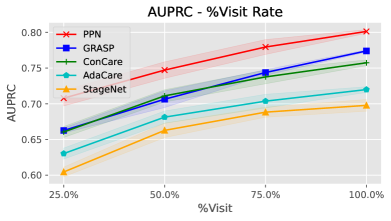
(a) Different visit rate

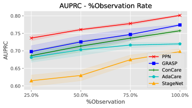
(b) Different observation rate

Fig. 2: Experiments on different visit rate and observation rate. The shadow represents the standard variance

4.5 Prototype Interpretations

To interpret the predictions, we illustrates the information about typical patients selected by PPN in Table 3. We found that each typical patient came from a different population, from young to old, male or female, diabetic or non-diabetic, showing their diversity.

For interpreting in the perspective of cohorts, we create a cohort set $\mathbb{S}_{j}$ for each typical patient $j$ containing all the patients whose most similar typical patient is $j$. Formally, $\mathbb{S}_{j}=\{i|s_{ij}>s_{ij^{\prime}},\forall j^{\prime}\neq j\}$, where $s_{ij}$ is the similarity between patient $i$ and typical patient $p_{j}$. Then we calculate the average age, male ratio, mortality rate, and diabetes rate in Table 4. The statistics among $\mathbb{S}_{j}$s are different, further confirming the diversity of prototypes learned by PPN. The similarity between patients and typical patients can be exploited for individual interpretation. We visualize the progression of the disease with the trajectory of changing cohorts of patients in the application so that physicians can understand the predictions.

Index	Age	Gender	Outcome	Diabetes	PD
#0	58.93	Male	Positive	True	DN
#1	62.07	Female	Negative	False	CIN
#2	42.28	Female	Positive	False	CGN
#3	44.94	Male	Positive	False	CGN
#4	79.44	Male	Negative	True	DN
#5	81.26	Female	Negative	True	DN

Table 3: Information of typical patients on the ESRD dataset. PD: primary disease. DN: diabetic nephropathy. CIN: chronic interstitial nephritis. CGN: chronic glomerulus nephritis.

Index	Avg. Age	Male Ratio	Mortality	Diabetes
#0	38.74	11.6%	9.5%	9.8%
#1	44.03	94.7%	18.2%	22.1%
#2	58.31	14.4%	35.1%	33.3%
#3	63.71	96.2%	42.3%	68.3%
#4	72.76	7.0%	56.3%	41.4%
#5	74.95	78.3%	76.1%	45.7%

Table 4: Statistics of $\mathbb{S}_{j}$ on the ESRD dataset

5 Conclusion

In this work, we propose a progressive prototypical network to select and incorporate information from typical patients. PPN adopts progressively selection and two separation losses to learn prototypes from the dataset while ensuring the cluster structure and diversity. We also design a prototypical feature integration to utilize their information to enhance the representation for the given patient. Experiments on three real-world datasets prove that PPN consistently outperforms state-of-the-art methods. Additional experiment demonstrate the effectiveness of PPN when handling patients with few visits and sparse records. Moreover, we develop an interactive application to illustrate the interpretable predictions for physicians. We hope our model can help physicians analyze patients through typical cases to diminish adverse outcomes.

Acknowledgement: This work was supported by the National Natural Science Foundation of China (No.82241052).

References

- [1] Huan Song, Deepta Rajan, Jayaraman Thiagarajan, and Andreas Spanias, “Attend and diagnose: Clinical time series analysis using attention models,” in Proceedings of the AAAI Conference on Artificial Intelligence, 2018, vol. 32.
- [2] Liantao Ma, Chaohe Zhang, Yasha Wang, Wenjie Ruan, Jiangtao Wang, Wen Tang, Xinyu Ma, Xin Gao, and Junyi Gao, “Concare: Personalized clinical feature embedding via capturing the healthcare context,” in Proceedings of the AAAI Conference on Artificial Intelligence, 2020, vol. 34, pp. 833–840.
- [3] Liantao Ma, Junyi Gao, Yasha Wang, Chaohe Zhang, Jiangtao Wang, Wenjie Ruan, Wen Tang, Xin Gao, and Xinyu Ma, “Adacare: Explainable clinical health status representation learning via scale-adaptive feature extraction and recalibration,” in Proceedings of the AAAI Conference on Artificial Intelligence, 2020, vol. 34, pp. 825–832.
- [4] Edward Choi, Mohammad Taha Bahadori, Joshua A Kulas, Andy Schuetz, Walter F Stewart, and Jimeng Sun, “Retain: An interpretable predictive model for healthcare using reverse time attention mechanism,” arXiv preprint arXiv:1608.05745, 2016.
- [5] Fenglong Ma, Radha Chitta, Jing Zhou, Quanzeng You, Tong Sun, and Jing Gao, “Dipole: Diagnosis prediction in healthcare via attention-based bidirectional recurrent neural networks,” in Proceedings of the 23rd ACM SIGKDD international conference on knowledge discovery and data mining, 2017, pp. 1903–1911.
- [6] Junyi Gao, Cao Xiao, Yasha Wang, Wen Tang, Lucas M Glass, and Jimeng Sun, “Stagenet: Stage-aware neural networks for health risk prediction,” in Proceedings of The Web Conference 2020, 2020, pp. 530–540.
- [7] Tian Bai, Shanshan Zhang, Brian L Egleston, and Slobodan Vucetic, “Interpretable representation learning for healthcare via capturing disease progression through time,” in Proceedings of the 24th ACM SIGKDD International Conference on Knowledge Discovery & Data Mining, 2018, pp. 43–51.
- [8] Amalia R Miller and Catherine Tucker, “Privacy protection and technology diffusion: The case of electronic medical records,” Management science, vol. 55, no. 7, pp. 1077–1093, 2009.
- [9] Jerome E Groopman and Michael Prichard, How doctors think, vol. 82, Houghton Mifflin Boston, 2007.
- [10] Alejandro Barredo Arrieta, Natalia Díaz-Rodríguez, Javier Del Ser, Adrien Bennetot, Siham Tabik, Alberto Barbado, Salvador García, Sergio Gil-López, Daniel Molina, Richard Benjamins, et al., “Explainable artificial intelligence (xai): Concepts, taxonomies, opportunities and challenges toward responsible ai,” Information Fusion, vol. 58, pp. 82–115, 2020.
- [11] Ganesh Raghu, Martine Remy-Jardin, Jeffrey L Myers, Luca Richeldi, Christopher J Ryerson, David J Lederer, Juergen Behr, Vincent Cottin, Sonye K Danoff, Ferran Morell, et al., “Diagnosis of idiopathic pulmonary fibrosis. an official ats/ers/jrs/alat clinical practice guideline,” American journal of respiratory and critical care medicine, vol. 198, no. 5, pp. e44–e68, 2018.
- [12] Hans-Joachim Anders, Tobias B Huber, Berend Isermann, and Mario Schiffer, “Ckd in diabetes: diabetic kidney disease versus nondiabetic kidney disease,” Nature Reviews Nephrology, vol. 14, no. 6, pp. 361–377, 2018.
- [13] Jake Snell, Kevin Swersky, and Richard S Zemel, “Prototypical networks for few-shot learning,” arXiv preprint arXiv:1703.05175, 2017.
- [14] Chaofan Chen, Oscar Li, Chaofan Tao, Alina Jade Barnett, Jonathan Su, and Cynthia Rudin, “This looks like that: deep learning for interpretable image recognition,” arXiv preprint arXiv:1806.10574, 2018.
- [15] Wenjia Xu, Yongqin Xian, Jiuniu Wang, Bernt Schiele, and Zeynep Akata, “Attribute prototype network for zero-shot learning,” arXiv preprint arXiv:2008.08290, 2020.
- [16] Guillaume Doras and Geoffroy Peeters, “A prototypical triplet loss for cover detection,” in ICASSP 2020-2020 IEEE International Conference on Acoustics, Speech and Signal Processing (ICASSP). IEEE, 2020, pp. 3797–3801.
- [17] David F Crouse, “On implementing 2d rectangular assignment algorithms,” IEEE Transactions on Aerospace and Electronic Systems, vol. 52, no. 4, pp. 1679–1696, 2016.
- [18] Tianqin Li, Zijie Li, Andrew Luo, Harold Rockwell, Amir Barati Farimani, and Tai Sing Lee, “Prototype memory and attention mechanisms for few shot image generation,” in International Conference on Learning Representations, 2022.
- [19] Oscar Li, Hao Liu, Chaofan Chen, and Cynthia Rudin, “Deep learning for case-based reasoning through prototypes: A neural network that explains its predictions,” in Proceedings of the AAAI Conference on Artificial Intelligence, 2018, vol. 32.
- [20] Chaohe Zhang, Xin Gao, Liantao Ma, Yasha Wang, Jiangtao Wang, and Wen Tang, “Grasp: Generic framework for health status representation learning based on incorporating knowledge from similar patients,” 2021.
- [21] Matthew A Reyna, Chris Josef, Salman Seyedi, Russell Jeter, Supreeth P Shashikumar, M Brandon Westover, Ashish Sharma, Shamim Nemati, and Gari D Clifford, “Early prediction of sepsis from clinical data: the physionet/computing in cardiology challenge 2019,” in 2019 Computing in Cardiology (CinC). IEEE, 2019, pp. Page–1.
- [22] Alistair EW Johnson, Tom J Pollard, Lu Shen, H Lehman Li-Wei, Mengling Feng, Mohammad Ghassemi, Benjamin Moody, Peter Szolovits, Leo Anthony Celi, and Roger G Mark, “Mimic-iii, a freely accessible critical care database,” Scientific data, vol. 3, no. 1, pp. 1–9, 2016.
- [23] Hrayr Harutyunyan, Hrant Khachatrian, David C Kale, Greg Ver Steeg, and Aram Galstyan, “Multitask learning and benchmarking with clinical time series data,” Scientific data, vol. 6, no. 1, pp. 1–18, 2019.
- [24] Frank Ruis, Gertjan Burghouts, and Doina Bucur, “Independent prototype propagation for zero-shot compositionality,” Advances in Neural Information Processing Systems, vol. 34, 2021.