Inducing Point Operator Transformer: A Flexible and Scalable Architecture for Solving PDEs

Abstract

Solving partial differential equations (PDEs) by learning the solution operators has emerged as an attractive alternative to traditional numerical methods. However, implementing such architectures presents two main challenges: flexibility in handling irregular and arbitrary input and output formats and scalability to large discretizations. Most existing architectures are limited by their desired structure or infeasible to scale large inputs and outputs. To address these issues, we introduce an attention-based model called an inducing-point operator transformer (IPOT). Inspired by inducing points methods, IPOT is designed to handle any input function and output query while capturing global interactions in a computationally efficient way. By detaching the inputs/outputs discretizations from the processor with a smaller latent bottleneck, IPOT offers flexibility in processing arbitrary discretizations and scales linearly with the size of inputs/outputs. Our experimental results demonstrate that IPOT achieves strong performances with manageable computational complexity on an extensive range of PDE benchmarks and real-world weather forecasting scenarios, compared to state-of-the-art methods.

Introduction

Partial differential equations (PDEs) are widely used for mathematically modeling physical phenomena by representing pairwise interactions between infinitesimal segments. Once formulated, PDEs allow us to analyze and predict the physical system, making them essential tools in various scientific fields (Strauss 2007). However, formulating accurate PDEs can be a daunting task without domain expertise where there remain numerous unknown processes for many complex systems. Moreover, traditional numerical methods for solving PDEs can require significant computational costs and may sometimes be intractable. In recent years, data-driven approaches have emerged as an alternative to the conventional procedures for solving PDEs, since they provide much faster predictions and only require observational data. In particular, operator learning, learning mapping between infinite-dimensional function spaces, generalizes well to unseen system inputs with their own flexibility in a discretization-invariant way (Lu et al. 2021, 2022; Kovachki et al. 2021; Li et al. 2020a, b, 2021b).

Observational data in solving PDEs often comes in much more diverse measurement formats, making it challenging to handle. These formats may include sparse and irregular measurements, different input and output domains, and complex geometries due to environmental conditions (Belbute-Peres, Economon, and Kolter 2020; Lienen and Günnemann 2022; Li et al. 2022; Tran et al. 2023). In addition, adaptive remeshing schemes are often deployed when different regions require different resolutions (Brenner, Scott, and Scott 2008; Huang and Russell 2010). However, most existing operator learners have their own restrictions. For instance, some require fixed discretization for the input function (Lu, Jin, and Karniadakis 2019; Lu et al. 2021), assume that input and output discretizations are the same (Lu et al. 2022; Li et al. 2020b, 2021b; Brandstetter, Worrall, and Welling 2022), assume local connectivity (Li et al. 2020a, b), or have uniform regular grids (Li et al. 2021b; Gupta, Xiao, and Bogdan 2021; Cao 2021). They can be limited when the observations have discrepancies between their own settings and given measurements. In order to be flexible to handle a variety of discretization schemes, the model should impose minimal assumptions on locality or data structure.

Our approach aims to address the challenges of handling arbitrary input and output formats by developing a mesh-agnostic architecture that treats observations as individual elements without problem-specific modifications. As flexible in processing data (Jaegle et al. 2021) and efficient in modeling long-range dependencies (Tsai et al. 2019), Transformer (Vaswani et al. 2017) can be an appropriate starting point for our approach. A core building block of the Transformers, the attention mechanism corresponds to and even outperforms the kernel integral operation of the existing operator learners due to its nature of capturing long-range interactions (Cao 2021; Liu, Xu, and Zhang 2022; Guo, Cao, and Chen 2023). However, their quadratic growth in computational complexity with input size can make it impractical for real-world applications, high-fidelity modeling, or long-term forecasting without imposing problem-specific locality.

To address the issue, we took inspiration from inducing-point methods which aim to reduce the effective number of input data points for computational efficiency (Quiñonero-Candela and Rasmussen 2005; Snelson and Ghahramani 2005; Titsias 2009; Li et al. 2020b), and from the extension of the methods to Transformer by cross-attention with a small number of learnable queries (Lee et al. 2019; Tang and Ha 2021; Jaegle et al. 2021, 2022; Rastogi et al. 2023). In this paper, we introduce a fully attention-based model called an inducing-point operator transformer (IPOT) to capture long-range interactions and provide flexibility for arbitrary input and output formats with feasible computational complexity. IPOT consists of an encoder-processor-decoder (Sanchez-Gonzalez et al. 2020; Pfaff et al. 2021), where the encoder compresses the input function into a smaller fixed number of latent bottlenecks inspired by inducing-point methods, the processor operates on the latent features, and the decoder produces solutions at any output queries from the latent features. This architecture achieves scalability by separating input and output discretizations from the latent processor. It allows the architecture to avoid quadratic complexity and decouples the depth of the processor from the size of the inputs or outputs. This approach can be used for real-world applications with large, complex systems or long-term forecasting tasks, making it feasible and practical to use.

Finally, we conducted several experiments on the extensive PDE benchmarks and a real-world dataset. Compared to state-of-the-art methods, IPOT achieves competitive performances with feasible computational complexity. It can handle uniform regular grids, irregular grids, real-world weather forecasting, and their variants with arbitrary discretization formats.

Related works

Operator learning. Based on a pioneer work (Chen and Chen 1995), deep operator networks (DeepONets) were presented to extend the architectures for operator learning with modern deep networks (Lu, Jin, and Karniadakis 2019; Lu et al. 2021). DeepONets consists of a branch network and a trunk network and can be queried out at any coordinate from the trunk network. However, they require the fixed discretization of the input functions from the branch network (Lu et al. 2022). Another promising framework is neural operators, which consist of several integral operators with parameterized kernels to map between infinite-dimensional functions (Kovachki et al. 2021; Li et al. 2020a, b, 2021b). Message passings on graphs (Li et al. 2020a, b; Pfaff et al. 2021), convolutions in the Fourier domain (Li et al. 2021b), or wavelets domain (Gupta, Xiao, and Bogdan 2021; Tripura and Chakraborty 2023) are used to approximate the kernel integral operations. However, the implemented architectures typically require having the same sampling points for input and output (Lu et al. 2022; Kovachki et al. 2021; Li et al. 2020b, 2021b). In addition, graph-based methods do not converge when problems become complex, and convolutional in the spectral domains methods are limited to the uniform regular grids due to the usage of FFT (Li et al. 2021b). To handle irregular grids, (Li et al. 2022; Tran et al. 2023) apply adaptive coordinate maps before and after FNO to make it extend to irregular meshes. Recently, Transformers have been recognized as flexible and accurate operator learners (Cao 2021). However, their quadratic scaling poses a significant challenge to their practical use. (Cao 2021) removes the softmax normalization and introduces Galerkin-type attention to achieve linear scaling. Although efficient transformers (Liu, Xu, and Zhang 2022; Li, Meidani, and Farimani 2022; Hao et al. 2023) have been proposed with preserving permutation symmetries (Lee 2022), the demand for flexibility and scalability is still not met for practical use in the real world.
Inducing-point methods. Inducing-point methods have been commonly used to approximate the Gaussian process through $m$ inducing points, where they involve replacing the entire dataset with smaller subsets that are representative of the data. These inducing points methods have been widely used in regression (Cao et al. 2013), kernel machines (Nguyen, Chen, and Lee 2021), and matrix factorizations (He and Xu 2019). A similar idea is also employed in the existing neural operator (Li et al. 2020b), which is based on graph networks and uses sub-sampled nodes from the original graph as inducing points to reduce the computational complexity of the previous graph neural operator (Li et al. 2020a). However, this approach did not converge for complex problems (Li et al. 2021b). Recently, the methods have been extended to Transformers by incorporating cross-attention with a reduced number of learnable query vectors (Lee et al. 2019; Tang and Ha 2021; Jaegle et al. 2021, 2022; Rastogi et al. 2023).

Preliminaries

Neural operators

Let us consider a set of $N$ input-output pairs, denoted by ${(a_{i},u_{i})}_{i=1}^{N}$, where $a_{i}=a_{i}|_{X}$ and $u_{i}=u_{i}|_{Y}$ are finite discretizations of the input function $a_{i}\in\mathcal{A}$ at the set of input points $X=\{x_{1},\ldots,x_{n_{x}}\}$ and output function $u_{i}\in\mathcal{U}$ at the set of output points $Y=\{y_{1},\ldots,y_{n_{y}}\}$ with the number of discretized points $n_{x}$ and $n_{y}$, respectively. Here, $\mathcal{A}$ and $\mathcal{U}$ are input and output function spaces, respectively. The objective of operator learning is to minimize the empirical loss $E_{a\sim\mu}\left[\mathcal{L}\left(\mathcal{G}_{\theta}(a),u\right)\right]\approx\frac{1}{N}\sum_{i=1}^{N}\|u_{i}-\mathcal{G}_{\theta}(a_{i})\|^{2}$ to learn a mapping $\mathcal{G}_{\theta}:\mathcal{A}\rightarrow\mathcal{U}$. The architectures of the neural operator (Kovachki et al. 2021; Li et al. 2021b), usually consist of three components, namely lifting, iterative updates, and projection, which correspond to the encoder-processor-decoder, respectively.

$$u=\mathcal{G}_{\theta}(a)=(\mathcal{Q}\circ\mathcal{G}_{L-1}\circ\dots\circ\mathcal{G}_{1}\circ\mathcal{P})(a)$$ (1)

where the lifting (encoder) $\mathcal{P}=\mathcal{G}_{enc}$ and projection (decoder) $\mathcal{Q}=\mathcal{G}_{dec}$ are local transformations that map input features to target dimensional features, implemented by point-wise feed-forward neural networks. The iterative updates $\mathcal{G}_{l}:v_{l}\mapsto v_{l+1},l\in[0,L-1]$ are global transformations that capture the interactions between the elements, implemented by a sequence of following transformations,

$$v_{l+1}(x)=\sigma\biggl{(}\mathcal{W}_{l}v_{l}(x)+\left[\mathcal{K}_{l}(v_{l})\right](x)\biggr{)},\quad x\in\Omega,$$ (2)

where $\sigma$ are nonlinear functions, $\mathcal{W}_{l}$ are point-wise linear transformations, $\mathcal{K}_{l}$ are kernel integral operations on $v_{l}(x)$. The existing implementations of the neural operators typically use the same discretizations for the input and output (Lu et al. 2022; Li et al. 2020b, 2021b; Brandstetter, Worrall, and Welling 2022), which leads to the predicted outputs only being queried at the input meshes. Our core idea is to replace the encoder $\mathcal{G}_{enc}$ and decoder $\mathcal{G}_{dec}$ to accommodate arbitrary size and structure of the input functions and output queries.

Kernel integral operation and attention mechanism

The kernel integral operations are generally implemented by integration of input values weighted by kernel values $\kappa$ representing the pairwise interactions between the elements on input domain $x\in\Omega_{x}$ and output domain $y\in\Omega_{y}$,

$$\left[\mathcal{K}(v)\right](y)=\int_{\Omega_{x}}\kappa(y,x)v(x)dx,\quad(x,y)\in\Omega_{x}\times\Omega_{y},$$ (3)

where the kernel $\kappa$ is defined on $\Omega_{y}\times\Omega_{x}$. The transform $\mathcal{K}$ can be interpreted as mapping a function $v(x)$ defined on a domain $x\in\Omega_{x}$ to the function $[\mathcal{K}(v)](y)$ defined on a domain $y\in\Omega_{y}$. Recently, it has been proved that the kernel integral operation can be successfully approximated by the attention mechanism of Transformers both theoretically and empirically (Kovachki et al. 2021; Cao 2021; Guibas et al. 2021; Pathak et al. 2022). Intuitively, let input vectors $X\in\mathbb{R}^{n_{x}\times d_{x}}$ and query vectors $Y\in\mathbb{R}^{n_{y}\times d_{y}}$, then the attention can be expressed as

$$\textsl{Attn}(Y,X,X)=\sigma(QK^{T})V\approx\int_{\Omega_{x}}(q(Y)\cdot k(x))v(x)dx,$$ (4)

where $Q=YW^{q}\in\mathbb{R}^{n_{y}\times d}$, $K=XW^{k}\in\mathbb{R}^{n_{x}\times d}$, $V=XW^{v}\in\mathbb{R}^{n_{x}\times d}$, and $\sigma$ are the query, key, value matrices, and softmax function, respectively. $W^{q}$, $W^{k}$, and $W^{v}$ are learnable weight matrices that operate in a pointwise way which makes the attention module not depend on the input and output discretizations. A brief derivation of Equation 4 can be found in the Appendix. The weighted sum of $V$ with the attention matrix $\sigma(QK^{T})$ can be interpreted as the kernel integral operation in which the parameterized kernel is approximated by the attention matrix (Tsai et al. 2019; Cao 2021; Xiong et al. 2021; Choromanski et al. 2021). This attention is also known as cross-attention, where the input vectors are projected to query embedding space by the attention, Attn$(Y,X,X)$. However, the computational complexity of the mechanism is proportional to $O(n_{x}n_{y}d)$, and it can cause quadratic complexity $O(n^{2}d)$ for large $n_{x}$ and $n_{y}$ ($n_{x},n_{y}\approx n$).

Approach

The goal of this work is to develop a mesh-agnostic architecture that can handle any input and output discretizations with reduced computational complexity. We allow for different, irregular, and arbitrary input and output formats.
Handling arbitrary input function and output queries. The output solution evaluated at output query $y$ can be expressed as $u(y)=\left[\mathcal{G}_{\theta}(a)\right](y)$ which can be viewed as the operating $\mathcal{G}:\mathcal{A}\times Y\rightarrow\mathcal{U}$ an input function $a\in\mathcal{A}$ at the corresponding output query $y\in Y$. We treat the representations of discretized input $a=a|_{X}\in\mathbb{R}^{n_{x}\times d_{a}}$, output $u=u|_{Y}\in\mathbb{R}^{n_{y}\times d_{u}}$ and corresponding output queries $Y\in\mathbb{R}^{n_{y}\times d_{y}}$ as sets of individual elements. In practice, they are represented by flattened arrays, without using structured bias to avoid our model bias toward specific data structures and flexibly process any discretization formats. The significant modifications from the existing neural operators (Equation 1) are mostly in the encoder and decoder for detaching the dependence of input and output discretizations by

$$Z_{0}=\mathcal{G}_{enc}(a),\quad Z_{l+1}=\mathcal{G}_{l}(Z_{l}),\quad\tilde{u}=\mathcal{G}_{dec}(Y,Z_{L}).$$ (5)

where the encoder projects the input function into latent space, the sequence of the processing is operated in latent space, and then the decoder predicts the output solutions from the latent representations at the corresponding output queries.
Positional encoding. In order to compensate for the positional information at each function value, we follow a common way of existing neural operators (Kovachki et al. 2021; Li et al. 2021b), which involves concatenating the position coordinates with the corresponding function values to form the input representation, $a=\{(x_{1},a(x_{1})),...,(x_{n_{x}},a(x_{n_{x}}))\}$. Additionally, instead of using raw position coordinates for both input $X=\{x_{1},...,x_{n_{x}}\}$ and outputs $Y=\{y_{1},...,y_{n_{y}}\}$, we concatenate additional Fourier embeddings for the position coordinates. This technique, which is commonly used to enrich positional information in neural networks (Vaswani et al. 2017; Mildenhall et al. 2020; Tancik et al. 2020; Sitzmann et al. 2020) involves exploiting sine and cosine functions with frequencies spanning from minimum to maximum frequencies, thereby covering the sampling rates for the corresponding dimensions.

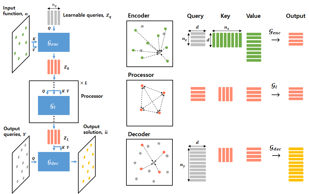
Figure 1: Inducing-point operator transformer (IPOT) uses a smaller number of inducing points, enabling it to flexibly handle any discretization formats of input and output, and significantly reduce the computational costs. IPOT encodes input function discretized on $X=\{x_{1},...,x_{n_{x}}\}$ to a fixed smaller size $n_{z}$ of learnable query vectors, and decoding them to output discretized on $Y=\{y_{1},...,y_{n_{y}}\}$. The number of size is varied as $n_{x}$ (arbitrary) → $n_{z}$ (fixed) → $n_{y}$ (arbitrary).

Inducing point operator transformer (IPOT)

We build our model with an attention-based architecture consisting of an encoder-processor-decoder, called an inducing point operator transformer (IPOT) to reduce the computational complexity of attention mechanisms (Figure 1). The key feature of IPOT is the use of a reduced number of inducing points ($n_{z}\ll n_{x},n_{y}$) (Lee et al. 2019; Jaegle et al. 2021; Rastogi et al. 2023). This is typically achieved by employing $n_{z}$ learnable query vectors into the encoder, allowing most of the attention mechanisms to be computed in the smaller latent space instead of the larger observational space. This results in a significant reduction in computational complexity. The encoder encodes the input function $a$ to the fixed smaller number of latent feature vectors (discretization number: ${n_{x}}\mapsto{n_{z}}$), the processor processes the pairwise interactions between elements of the latent features vectors (discretization number: ${n_{z}}\mapsto{n_{z}}$), and the decoder decodes the latent features to output solutions at a set of output queries $Y$ (discretization number: ${n_{z}}\mapsto{n_{y}}$).
Attention blocks. The exact form of the attention blocks Attention$(Y,X,X)$ used in the following sections are described in Appendix.The nonlinearity $\sigma$, pointwise linear transformations $\mathcal{W}_{l}$, and kernel integral operations $\mathcal{K}_{l}$ in Equation 2 are approximated by feed-forward neural networks, residual connections, and the attention modules, which are common block forms of Transformer-like architectures (Vaswani et al. 2017). In addition, layer normalization (Ba, Kiros, and Hinton 2016) is used to normalize the query, key, and values inputs, and multi-headed extensions of the attention blocks can be optionally employed to improve the model’s performance.
Encoder. We use a cross-attention block as the encoder to encode inputs $a$ with the size $n_{x}$ to a smaller fixed number $n_{z}$ of learnable query vectors (inducing points) $Z_{q}\in\mathbb{R}^{n_{z}\times d_{z}}$ (typically $n_{z}\ll n_{x}$). Then the result of the block is

$$Z_{0}=\mathcal{G}_{enc}(a)=\textsl{Attention}(Z_{q},a,a)\in\mathbb{R}^{n_{z}\times d_{z}},$$ (6)

where each learnable query vector of $Z_{q}$ is randomly initialized by a normal distribution and learned along the architectures. The encoder maps the input domain to a latent domain consisting of $n_{z}$ inducing points based on the correlations between input discretizations and inducing points. The computational complexity of the encoder is proportional to $O(n_{x}n_{z}d)$ which scales linearly with the input size $n_{x}$. Furthermore, the use of inducing points reduces the computational complexity of the subsequent attention blocks.
Processor. We use a series of self-attention blocks as the processor each of which takes $Z_{l}\in\mathbb{R}^{n_{z}\times d_{z}}$ as the input of the query, key, and value components. Then the output of each self-attention block for $l\in[0,L-1]$ is

$$Z_{l+1}=\mathcal{G}_{l}(Z_{l})=\textsl{Attention}(Z_{l},Z_{l},Z_{l})\in\mathbb{R}^{n_{z}\times d_{z}},$$ (7)

which captures global interactions of inducing points in the latent space. Since the processor is decoupled from the input and output discretizations, IPOT is not only applicable to any input and output discretization formats but also significantly reduces computational costs. Processing in the latent space rather than in observational space reduces the costs in the processor to $O(Ln_{z}^{2}d)$ from $O(Ln_{x}^{2}d)$ for the original Transformers. This decouples the depth of the processor $L$ from the size of input $n_{x}$ or output $n_{y}$, allowing the construction of deep architectures or long-term forecasting models with large $L$.
Decoder. We use a cross-attention block as the decoder to decode the latent vectors from the processor $Z_{L}\in\mathbb{R}^{n_{z}\times d_{z}}$ at output queries $Y\in\mathbb{R}^{n_{y}\times d}$. Then, the output solutions predicted by IPOT at the corresponding output queries are

$$\tilde{u}=\mathcal{G}_{dec}(Y,Z_{L})=\textsl{Attention}(Y,Z_{L},Z_{L})\in\mathbb{R}^{n_{y}\times d_{u}}.$$ (8)

The decoder maps the latent domain to the output domain based on the correlations between $n_{z}$ inducing points and output queries $Y$. Since the result from the processor is independent of the discretization format of input function $a$, the entire model is also applicable to arbitrary input discretization and can be queried out at arbitrary output queries. In addition, the computational cost of the decoder is proportional to $O(n_{z}n_{y}d)$ which also scales linearly with the output size $n_{y}$.

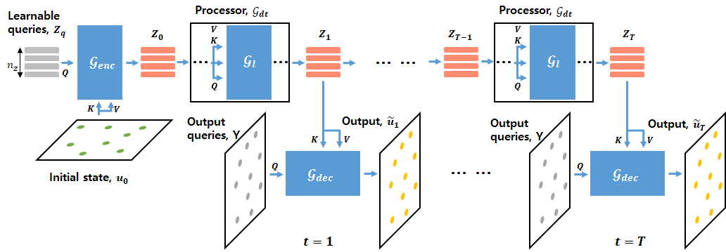
Figure 2: The state of the system at time $T$ is denoted as $u_{T}=(\mathcal{G}_{dec}\circ[\mathcal{G}_{dt}\circ\cdots\circ\mathcal{G}_{dt}]\circ\mathcal{G}_{enc})(u_{0})$, where $\mathcal{G}_{enc}$ is an encoder that maps the initial state $u_{0}$ to the latent state, $\mathcal{G}_{dec}$ is a decoder that maps the latent state back to the observational state, and $\mathcal{G}_{dt}$ is a processor that steps forward in time by $dt$ implemented by a series of self-attention blocks on latent states.

Time-stepping through latent space

We model the time-dependent PDEs as an autoregressive process. The state of the system at time $t+dt$ is described as $u_{t+dt}=(\mathcal{G}_{dec}\circ\mathcal{G}_{dt}\circ\mathcal{G}_{enc})(u_{t})$, where $\mathcal{G}_{enc}$ is an encoder that maps the current observational state to the latent state, $\mathcal{G}_{dec}$ is a decoder that maps the latent state back to the observational state, and $\mathcal{G}_{dt}$ is a processor that steps forward in time by $dt$ implemented by a series of self-attention blocks on the latent states. We assume that the processor $\mathcal{G}_{dt}$ is independent of $t$ (Sanchez-Gonzalez et al. 2020; Pfaff et al. 2021; Li et al. 2021a; Li, Meidani, and Farimani 2022). When setting the time step as $dt=1$, the predicted trajectory of the system is obtained by the following recurrent relation at each time $t\in[0,T-1]$

$$Z_{0}=\mathcal{G}_{enc}(u_{0}),\quad Z_{t+1}=\mathcal{G}_{dt}(Z_{t}),\quad\tilde{u}_{t+1}=\mathcal{G}_{dec}(Y,Z_{t+1}).$$ (9)

where $u_{0}$ is the initial state, $Y$ are output queries, and identical processor $\mathcal{G}_{dt}$ is applied at each time step. Throughout the entire trajectory, by encoding the initial state into the latent space, we can significantly reduce the computational costs of subsequent processing compared to processing in the observational space.

Computational complexity

The overall computational complexity of IPOT is proportional to $O(n_{x}n_{z}d+Ln_{z}^{2}d+n_{z}n_{y}d)$ which scales linearly to $n_{x}$ and $n_{y}$, and the depth of architecture $L$ is decoupled from the input and output size. When $n_{x},n_{y}\approx n$ and $L\gg 1$, the complexity becomes $O(Ln_{z}^{2}d+2nn_{z}d)\approx O(Ln_{z}^{2}d)$, which is significantly lower than that of standard Transformer $O(Ln^{2}d)$ (Vaswani et al. 2017), which has quadratic scaling and is coupled with $L$. Existing operator learners including Fourier neural operator $O(Ln\log{n}\,d)$ (Li et al. 2021b) or linear Transformers $O(Lnd^{2})$ (Cao 2021; Li, Meidani, and Farimani 2022) have sub-quadratic scaling with the size $n$, but they are coupled with the depth $L$. The decoupling of the depth $L$ from the size $n$ makes it practical to construct deep architectures or apply them to long-term forecasting that requires a large $L$.

Experiments

We conduct experiments on several benchmark datasets, including PDEs on regular grids (Li et al. 2021b), irregular grids (Li et al. 2022; Tran et al. 2023; Yin et al. 2022), and real-world data from the ERA5 reanalysis dataset (Hersbach et al. 2020) to investigate the flexibility and scalability of our model through various downstream tasks. Details of the equations and the problems are described in Appendix.Results for experiments already discussed on baselines were obtained from the related literature, and results for the extended tasks that have not been discussed before have been reproduced from their original codes. We provide some illustrations of the predictions of IPOT for the benchmarks on regular and irregular grids (Figure 3) and for long-term dynamics (Figure 4). The implementation details and additional results can be found in the Appendix.
Baselines. We took several representative architectures as baselines including deep operator network (DeepONet) (Lu, Jin, and Karniadakis 2019), the mesh-based learner with graph neural networks (Meshgraphnet) (Pfaff et al. 2021), Fourier neural operator (FNO) (Li et al. 2021b), Factorized-Fourier neural operator (FFNO) (Tran et al. 2023), and operator Transformer (OFormer) (Li, Meidani, and Farimani 2022).
Evaluation metric. We use relative $L_{2}$ error for the objective functions and evaluation metrics for test errors, where we follow the convention of related literature (Kovachki et al. 2021; Li et al. 2021b). When $N$ is the dataset size of input-output pairs $(a_{i},u_{i})_{i=1}^{N}$, the relative $L_{2}$ error is defined as

$$E_{a\sim\mu}[\mathcal{L}(\mathcal{G}_{\theta}(a),u)]=\frac{1}{N}\sum_{i=1}^{N}\frac{\|u-\mathcal{G}_{\theta}(a)\|_{2}}{\|u_{i}\|_{2}}.$$ (10)

Problems of PDEs solved on regular grids

We conducted experiments on benchmark problems, where the PDEs for Darcy flow, and Navier-Stokes equation were solved on regular grids from (Li et al. 2021b). Shown in Table 1, IPOT consistently demonstrates competitive or strong performances with efficient computational resources, particularly in the case of Navier-Stokes benchmarks that involve higher complexity and time-dependence, resulting in larger $n$ and requiring models with long sequences $L$ of processors or iterative updates. These achievements are obtained without using any problem-specific layers such as pooling layers or convolutional filters, which are only compatible the regular grid structures. Consequently, IPOT offers greater flexibility in handling arbitrary inputs and output formats beyond the regular grids.

Problems of PDEs solved on irregular grids

In addition, we conducted experiments on various problems, where the PDEs were solved on non-uniform and irregular grids. These problems include predicting flows around complex geometries (airfoil), estimating stresses on irregularly sampled point clouds (elasticity), and predicting displacements given initial boundary conditions for plastic forging problem (plasticity) as described in (Tran et al. 2023). The experimental results presented in Table 1 also demonstrate that our IPOT model demonstrates competitive or stronger performances with efficient computational resources, as illustrated in Figure 3.

Table 1: Performance and efficiency comparisons with baselines across various datasets. The efficiencies are compared in terms of the number of parameters, time spent per epoch (seconds), and CUDA memory consumption (GB). The missing entries occur when the methods are not able to handle the datasets or when encountering convergence issues.

Dataset	Model	Params	Runtime	Memory	Error
Darcy Flow	DeepONet	0.42M	2.73	2.40	4.61e-2
	Meshgraphnet	0.21M	9.51	5.57	9.67e–2
	FNO	1.19M	1.88	1.96	1.09e–2
	FFNO	0.41M	3.36	1.99	7.70e–3
	OFormer	1.28M	3.63	5.71	1.26e–2
	IPOT (ours)	0.15M	2.70	1.82	1.73e–2
Navier Stokes	DeepONet	-	-	-	-
	Meshgraphnet	0.29M	137.17	6.15	1.29e–1
	FNO	0.93M	53.73	3.09	1.28e–2
	FFNO	0.27M	53.82	3.40	1.32e–2
	OFormer	1.85M	70.15	9.90	1.04e–2
	IPOT (ours)	0.12M	21.05	2.08	8.85e–3
Airfoil	DeepONet	0.42M	3.13	2.75	3.85e–2
	Meshgraphnet	0.22M	10.92	6.38	5.57e–2
	FNO	1.19M	2.63	2.73	4.21e–2
	FFNO	0.41M	4.71	2.78	7.80e–3
	OFormer	1.28M	4.17	7.97	1.83e–2
	IPOT (ours)	0.12M	2.15	2.10	8.79e–3
Elasticity	DeepONet	1.03M	3.72	1.18	9.65e–2
	Meshgraphnet	0.46M	7.36	4.04	4.18e–2
	FNO	0.57M	1.04	1.68	5.08e–2
	FFNO	0.55M	2.42	2.08	2.63e–2
	OFormer	2.56M	5.58	2.98	1.83e–2
	IPOT (ours)	0.12M	1.99	1.13	1.56e–2
Plasticity	DeepONet	-	-	-	-
	Meshgraphnet	-	-	-	-
	FNO	1.85M	10.40	16.81	5.08e–2
	FFNO	0.57M	66.47	16.86	4.70e–3
	OFormer	0.49M	28.43	14.11	1.83e–2
	IPOT	0.13M	10.14	5.35	3.25e–3
ERA5	DeepONet	-	-	-	-
	Meshgraphnet	2.07M	51.75	18.45	7.16e–2
	FNO	2.37M	9.23	13.04	1.21e–2
	FFNO	1.12M	14.39	17.06	7.25e–3
	OFormer	1.85M	71.18	10.90	1.15e–2
	IPOT (ours)	0.51M	9.83	10.58	6.64e–3

Application to real-world data

Unlike the previous problems, we conducted experiments on a subset of the ERA5 reanalysis dataset from the European Centre for Medium-Range Weather Forecasts (ECMWF) (Hersbach et al. 2020), where the governing PDEs are unknown. While the ERA5 database includes extensive hourly and monthly measurements for a number of parameters at various pressure levels, our focus is specifically on predicting the daily temperature at 2m from the surface $T_{2m}$. IPOT also achieves superior accuracy compared to the baselines while maintaining comparable both time and memory costs. Using the decoupled $n_{z}$ inducing points from the observational space, our approach mitigates the computational burden associated with large $n$ and $L$, making it beneficial for complex and long-term forecasting tasks.
Generalization ability on discretizations. Furthermore, we explore the model’s generalization ability to different resolutions and to make predictions from partially observed inputs. The evaluation of different resolutions is motivated by the scenario where observations are collected at varying resolutions. The evaluation with masked inputs is motivated by situations when observations are only available for the sea surface while data from land areas are unavailable as shown in the bottom right of Figure 4. We employ bilinear interpolation methods to obtain interpolated input values corresponding to land coordinates and combine them with the masked inputs for some comparison models that necessitate a consistent grid structure for both input and output data. As shown in Table 2, IPOT consistently outperforms all the baselines in all scenarios, demonstrating stable and strong performance. These results highlight the exceptional flexibility and accuracy of IPOT, showcasing its remarkable generalization capability.

Table 2: Performance results for comparing the generalization ability on discretizations. The models are evaluated on the task of different resolutions and masked inputs for the ERA5 dataset.

Model	Different resolutions			Partial observed
	res$=4^{\circ}$	res$=1^{\circ}$	res$=0.25^{\circ}$	Masked land
FNO	1.30e–2	1.23e–2	1.24e–2	3.10e–2
OFormer	3.66e–2	1.65e–2	1.86e–2	4.37e–2
IPOT (ours)	8.96e–3	7.78e–3	8.66e–3	2.83e–2

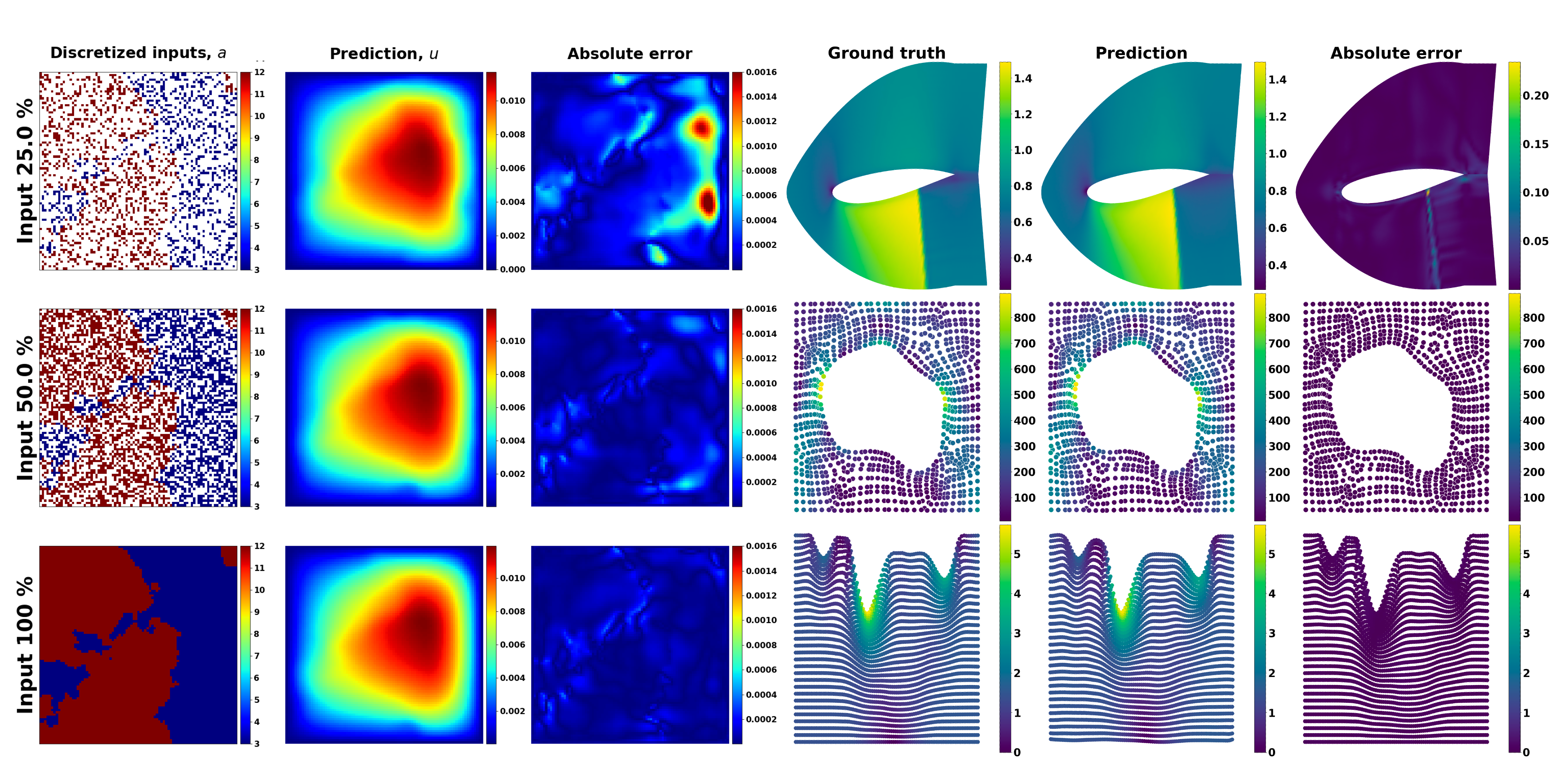
Figure 3: Predictions of IPOT on the problems of Darcy flow (left), airfoil (top right), elasticity (middle right), and plasticity (bottom right). In the case of Darcy flow, the partially observed inputs are randomly subsampled with the ratios of $\{100,50,25\}\%$.

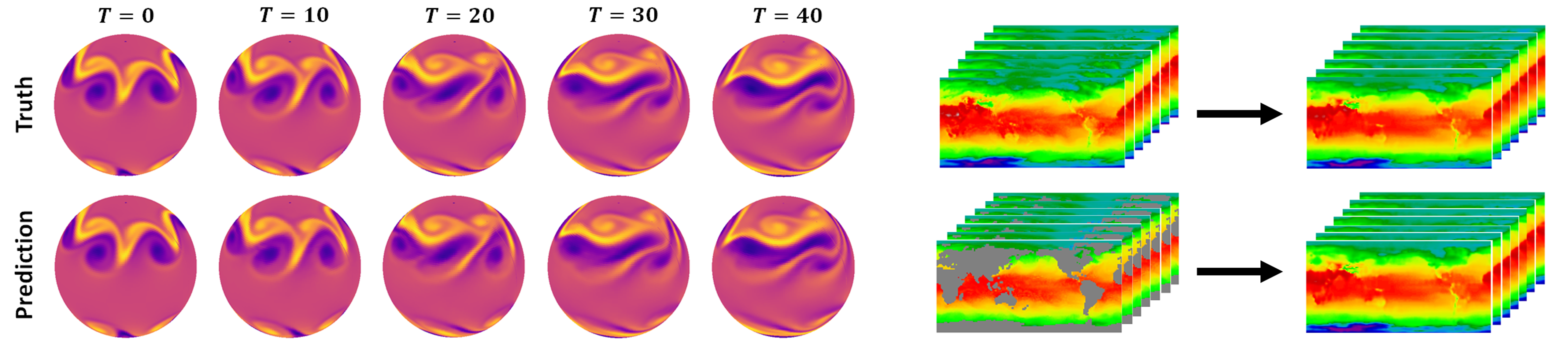
Figure 4: Long-term predictions of IPOT on spherical manifolds for the shallow-water equations (left), and on real-world weather forecasting when the inputs are spatially fully given (top right), and partially given (bottom right).

Ablation study

Effect of the number of inducing points. We conducted experiments on ERA5 data with varying numbers of latent query vectors, ranging from 64 to 512, to evaluate the effect of the number of inducing points, and to emulate the quadratic complexity in attention blocks of the standard Transformer (Vaswani et al. 2017), we also consider IPOT without inducing points. In this variant, we use self-attention where the observational input is injected into query, key, and value components instead of using cross-attention with learnable queries in the encoder. Table 3 demonstrates that increasing the number of latent query vectors improves the performance of IPOT. Notably, when the number is over 256, IPOT sufficiently outperforms other baselines. However, when the number of inducing points is too small, IPOT exhibits poor performance. Additionally, the quadratic complexity of attention in a standard Transformer hinders convergence and results in excessive computational time.

Table 3: Performance of IPOT with varying the number of inducing points. IPOT w.o ip denotes that IPOT without inducing points which emulates the standard Transformer.

Model	$n$	$n_{z}$	$L$	Runtime	Error	Complexity
OFormer	16.2K	16.2K	19	71.18	1.15e–2	$\mathcal{O}(Lnd^{2})$
IPOT w.o ip	16.2K	16.2K	28	$\gg 100$	–	$\mathcal{O}(Ln^{2}d)$
IPOT (64)	16.2K	64	28	7.44	1.45e–2	$\mathcal{O}(Ln_{z}^{2}d)$
IPOT (128)	16.2K	128	28	7.61	1.30e–2	$\mathcal{O}(Ln_{z}^{2}d)$
IPOT (256)	16.2K	256	28	7.91	6.87e–3	$\mathcal{O}(Ln_{z}^{2}d)$
IPOT (512)	16.2K	512	28	9.83	6.44e–3	$\mathcal{O}(Ln_{z}^{2}d)$

Computational complexity on different resolutions. We compared the computational complexity of different models on the ERA5 data at different resolutions, as shown in Figure 5. The time complexities were assessed by measuring the inference time in seconds for processing observational data during testing, and the memory complexities were evaluated by recording CUDA memory allocation. It is observed that IPOT without latent inducing points, which serves as a surrogate for a standard Transformer with quadratic complexity in self-attention, does not scale well in terms of both time and memory costs. IPOT with 256 or 512 inducing points scale effectively up to $n=10^{6}$, making them suitable for handling large-scale observational data due to their efficiency in both time and memory complexity.

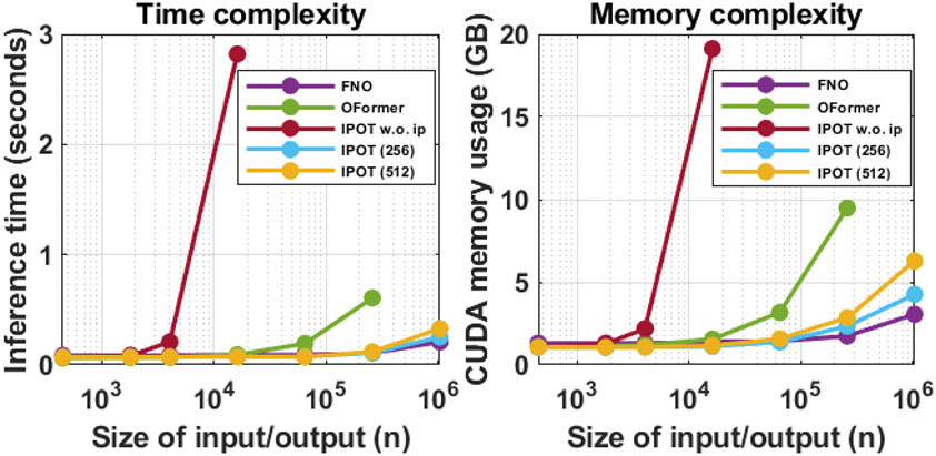
Figure 5: Complexity comparisons on different resolutions. We compare the different models in terms of inference time (left) and CUDA memory usage (right) with different sizes of input/output.

Conclusions

In this work, we raise potential issues on existing operator learning models for solving PDEs in terms of flexibility in handling irregular and arbitrary input and output discretizations, as well as the computational complexity for complex and long-term forecasting real-world problems. To address these issues, we propose IPOT, an attention-based architecture capable of handling arbitrary input and output discretizations while maintaining feasible computational complexity. This is achieved by using a reduced number of inducing points in the latent space, effectively addressing the quadratic scaling issue in the attention mechanism. Our proposed model demonstrates superior performance on a wide range of benchmark problems, including PDEs solved on both regular and irregular grids. Furthermore, we show that IPOT outperforms other baseline models on real-world data with competitive efficiency. Moreover, IPOT exhibits strong generalization ability, providing consistent performance in challenging real-life scenarios, while other models often suffer from significant performance degradation or require additional pre-processing for compatibility with the data structure.

Additional related Works

Learning-based PDE solvers. Recently, modern deep-learning techniques have shown great promise in solving PDEs. One popular direction is the physics-informed neural networks (PINNs) (Raissi, Perdikaris, and Karniadakis 2019; Karniadakis et al. 2021), which use implicit neural representations (INRs) (Sitzmann et al. 2020) to solve PDEs given boundary conditions and collocation points constrained to known governing equations. While PINNs yield mesh-agnostic and high-fidelity solutions, they require full knowledge of the PDEs and cannot be reused for new boundary conditions. Another research direction attempts to predict flow fields around various shapes using the PointNet (Qi et al. 2017) on complex irregular grids (Kashefi, Rempe, and Guibas 2021), which was later extended to include physics constraints (Kashefi and Mukerji 2022). Additionally, (Jiang et al. 2020; Bode et al. 2021) encodes low-resolution inputs to latent contexts and feeds them to decoding networks to predict solutions at output queries. While these methods were originally formulated for super-resolution problems and use physics constraints, our proposed approach is designed for operator learning problems. Similar to our work, mesh-agnostic approaches without any physics constraints have been achieved by (Pan, Brunton, and Kutz 2022; Yin et al. 2022) using INRs conditioned on hypernetworks (Ha, Dai, and Le 2016). They built their architecture upon INRS, whereas our approach is built upon Transformers.

Derivation of equation 4

Here is a brief explanation of the approximation with the integral for the cross-attention mechanism, where the softmax for the attention matrix is ignored for simplicity.

$$\textsl{Attn}(Y,X,X)=\begin{bmatrix}\textsl{Attn}(y_{1},X,X)\\ \vdots\\ \textsl{Attn}(y_{n_{y}},X,X)\end{bmatrix}$$ (11)

$$=\begin{bmatrix}q(y_{1})\\ \vdots\\[15.0pt] q(y_{n_{y}})\end{bmatrix}\begin{bmatrix}k_{1}(x_{1})&\ldots&k_{1}(x_{n_{x}})\\ \vdots&\ddots&\vdots\\[15.0pt] k_{d_{q}}(x_{1})&\ldots&k_{d_{q}}(x_{n_{x}})\end{bmatrix}\begin{bmatrix}v(x_{1})\\ \vdots\\ v(x_{n_{x}})\end{bmatrix}$$

$$=\begin{bmatrix}q(y_{1})\cdot k(x_{1})&\ldots&q(y_{1})\cdot k(x_{n_{x}})\\ \vdots&\ddots&\vdots\\ q(y_{n_{y}})\cdot k(x_{1})&\ldots&q(y_{n_{y}})\cdot k(x_{n_{x}})\end{bmatrix}\begin{bmatrix}v(x_{1})\\ \vdots\\ v(x_{n_{x}})\end{bmatrix}$$

$$=\begin{bmatrix}\sum_{i=1}^{n_{x}}(q(y_{1})\cdot k(x_{i}))v(x_{i})\\ \vdots\\ \sum_{i=1}^{n_{x}}(q(y_{n_{y}})\cdot k(x_{i}))v(x_{i})\end{bmatrix}$$

$$\approx\begin{bmatrix}\int_{\Omega_{x}}(q(y_{1})\cdot k(x))v(x)dx\\ \vdots\\ \int_{\Omega_{x}}(q(y_{n_{y}})\cdot k(x))v(x)dx\end{bmatrix}=\int_{\Omega_{x}}(q(Y)\cdot k(x))v(x)dx.$$

Here, the discretization of input is $\{x_{1},...,x_{n_{x}}\}$ (as key and value vectors), and it can be changed to the discretization of output $\{y_{1},...,y_{n_{y}}\}$ (as query vectors) with cardinality changed from $n_{x}$ to $n_{y}$. Using this mechanism, we can detach the dependences of discretization formats of input and output from the processor, by encoding arbitrary discretization $\{x_{1},...,x_{n_{x}}\}$ to a fixed size ($n_{z}$) of learnable latent set vectors, and decoding the latent set vectors to output arbitrary discretization $\{y_{1},...,y_{n_{y}}\}$. The discretization number is varied as $n_{x}$ (arbitrary) $\rightarrow$ $n_{z}$ (fixed) $\rightarrow$ $n_{y}$ (arbitrary).

Attention blocks

Mesh-independent neural operator (IPOT) consists of two types of attention blocks, cross- and self-attention blocks, which implement the respective attention mechanisms. The attention blocks have the shared structures following the Transformer-style architectures (Vaswani et al. 2017; Jaegle et al. 2021, 2022), which takes two input arrays, a query input $Y\in\mathbb{R}^{n_{y}\times d_{y}}$ and a key-value input $X\in\mathbb{R}^{n_{x}\times d_{x}}$,

$$O=Y+\textsl{Attn}(\textsl{LN}(Y),\textsl{LN}(X),\textsl{LN}(X)),$$ (12)

$$\textsl{Attention}(Y,X,X)=O+\textsl{FF}(\textsl{LM}(O)),$$

where LN is layer normalization (Ba, Kiros, and Hinton 2016), FF consists of two point-wise feedforward neural networks with a GELU nonlinearity (Hendrycks and Gimpel 2016), and the exact calculation of attention Attn is

$$\textsl{Attn}(X^{q},X^{k},X^{v})=\textsl{Softmax}\left(\frac{QK^{T}}{\sqrt{d_{q}}}\right)V,$$ (13)

where $Q=X^{q}W^{q}\in\mathbb{R}^{n_{y}\times d_{q}}$, $K=X^{k}W^{k}\in\mathbb{R}^{n_{x}\times d_{q}}$, and $V=X^{v}W^{v}\in\mathbb{R}^{n_{x}\times d_{v}}$ for a single headed attention. In the case of multi-headed attention, several outputs from different learnable parameters are concatenated and projected with the linear transformation.

Datasets

In this section, we present an overview of the datasets and describe the corresponding equations and tasks along with the details of inputs and outputs. Table 4 presents a summary of the datasets for easy reference across different domains, including problems of PDEs solved on regular grids, irregular grids, and real-world data. The footnotes of each problem set are the corresponding URL addresses for the datasets, which are publicly available. The train/test split settings are also directly taken from respective benchmark datasets.

Table 4: Overview of datasets and the corresponding tasks in terms of size of input and output.

Dataset	Problem	Input	Output	Input size	Output size
Burgers	1D regular grid	$u(\cdot,0)$	$u(\cdot,1)$	1,024$\times$1	1024$\times$1
Darcy flow	2D regular grid	$a$	$u$	7,225$\times$1	7,225$\times$1
Navier-Stokes, $\nu{=}$1e–3	2D regular grid	$w(\cdot,t)|_{t\in[0,10]}$	$w(\cdot,t)|_{t\in(10,50]}$	4,096$\times$10	4,096$\times$1$\times$40
Navier-Stokes, $\nu{=}$1e–4	2D regular grid	$w(\cdot,t)|_{t\in[0,10]}$	$w(\cdot,t)|_{t\in(10,30]}$	4,096$\times$10	4,096$\times$1$\times$20
Navier-Stokes, $\nu{=}$1e–5	2D regular grid	$w(\cdot,t)|_{t\in[0,10]}$	$w(\cdot,t)|_{t\in(10,20]}$	4,096$\times$10	4,096$\times$1$\times$10
Airfoil	Transonic flow	Mesh point	Velocity	11,271$\times$2	11,271$\times$1
Elasticity	Hyper-elastic material	Point cloud	Stress	972$\times$2	972$\times$1
Plasticity	Plastic forging	Boundary condition	Displacement	62,620$\times$1	62,620$\times$4
Spherical shallow water	Spherical manifold	$u(\cdot,0)$	$u(\cdot,t)|_{t\in(0,20]}$	8,192$\times$2	8,192$\times$2$\times$19
ERA5	[Train] $T_{2m}$ forecasting	$u(\cdot,t)|_{t\in[-6,0]}$	$u(\cdot,t)|_{t\in[1,7]}$	16,200$\times$7	16,200$\times$1$\times$7
ERA5	[Test] Masked land	$u(\cdot,t)|_{t\in[-6,0]}$	$u(\cdot,t)|_{t\in[1,7]}$	11,105$\times$7	16,200$\times$1$\times$7
ERA5	[Test] Masked sea	$u(\cdot,t)|_{t\in[-6,0]}$	$u(\cdot,t)|_{t\in[1,7]}$	5,095$\times$7	16,200$\times$1$\times$7

Problems of PDEs solved on regular grids

Burgers’ equation. Burgers’ equation is a non-linear parabolic PDE combining the terms of convection and diffusion. The benchmark problem of 1D Burgers’ equation with periodic boundary conditions is defined as

$$\partial_{t}u(x,t)+\partial_{x}(u^{2}(x,t)/2)=\nu\partial_{xx}u(x,t),$$

$$\qquad\qquad\!\!\ u(x,0)=u_{0}(x),$$

where $u_{0}\sim\mu$ is the initial state generated from $\mu=\mathcal{N}(0,625(-\Delta+25I)^{-2})$ and $\nu=0.1$ is the viscosity coefficient. The goal of operator learning is to learn mapping the initial state to the solution at $t=1$, $\mathcal{G}:u(\cdot,0)\mapsto u(\cdot,1)$. During training, the input and output discretizations are given at 1,024 equispaced grids.
Darcy flowregular. Darcy flow is a second-order elliptic PDE describing the flow of fluid through a porous medium. The benchmark problem of 2D steady-state Darcy flow on unit cell is defined as

$$-\nabla\cdot(a(x)\nabla u(x))=f(x),$$

$$u(x)=0,$$

where $u$ is density of the fluid, $a\sim\mu$ is the diffusion field generated from $\mu=\mathcal{N}(0,(-\Delta+9I)^{-2})$ with fixed forcing function $f=1$. The goal of operator learning is to learn mapping the diffusion field to the solution of the density, $\mathcal{G}:a\mapsto u$. During training, the discretizations of input and output are sampled at 85${\times}$85${=}$7,225 regular grids.
Navier-Stokes equationregular. Navier-Stokes equation describes the dynamics of a viscous, incompressible fluid. The benchmark problem of the 2D Navier-Stokes equation in vorticity form on the unit torus is defined as

$$\ \partial_{t}w(x,t)+u(x,t)\cdot\nabla w(x,t)=\nu\Delta w(x,t)+f(x),$$

$$\nabla\cdot u(x,t)=0,$$

$$w(x,0)=w_{0}(x),$$

where $u$ is the velocity field, $w=\nabla\times u$ is the vorticity field, $w_{0}\sim\mu$ denotes the initial vorticity field generated from $\mu=\mathcal{N}(0,7^{3/2}(-\Delta+49I)^{-2.5})$ with periodic boundary conditions, and the forcing function is kept $f(x)=0.1\left(\sin\left(2\pi\left(x_{1}+x_{2}\right)\right)+\cos\left(2\pi\left(x_{1}+x_{2}\right)\right)\right)$. The goal of operator learning is to learn the mapping from the initial times $t\in[0,10]$ of the vorticity fields to further trajectories up to $t=T$, defined by $w(\cdot,t)|_{t\in[0,10]}\mapsto w(\cdot,t)|_{t\in(10,T]}$. The time total duration of each trajectory is $T{=}$50, 30, and 10 corresponding to the viscosity coefficients $\nu{=}$1e–3, 1e–4, and 1e–5, respectively, for each dataset (Li et al. 2021b). 1,000 instances are used for training and 100 for testing. During both training and testing, the spatial discretizations of input and output are sampled at 65${\times}$65${=}$4,096 regular grids.

Problems of PDEs solved on irregular grids

Airfoil. The benchmark problem of the airfoil is based on the transonic flow over an airfoil, which is governed by Euler’s equation. The equation is defined as

$$\partial_{t}\rho+\nabla\cdot(\rho^{f}v)=0,$$ (14)

$$\partial_{t}(\rho u)+\nabla\cdot(\rho u\otimes u+pI)=0,$$

$$\partial_{t}E+\nabla\cdot\big{(}(E+p)u\big{)}=0,$$

where $\rho$ is the density, $u$ is the velocity field, $p$ is the pressure, and $E$ is the total energy. The far-field boundary conditions are $\rho_{\infty}=1,p_{\infty}=1$, and Mach number $M_{\infty}=0.8$, with no penetration imposed at the airfoil. The shape and mesh grids of the datasets used in this study are adopted from (Li et al. 2022), which consists of variations of the NACA-0012 airfoils. The dataset is split into 1,000 instances for training and 200 instances for testing. The inputs and outputs are given as the mesh grids and the corresponding velocities in terms of Mach number.
Elasticityirregular. The benchmark problem of elasticity involves hyper-elastic material, which is governed by constitutive equations. The equation on the bounded unit cell $\Omega\in[0,1]^{2}$ is defined as

$$\rho\frac{\partial^{2}u}{\partial t^{2}}+\nabla\cdot\sigma=0,$$ (15)

where $\rho$ is mass density, $u$ is the displacement vector, and $\sigma$ is the stress tensor, respectively. The random-shaped cavity at the center has a radius that is sampled as $r=0.2+\frac{0.2}{1+\exp(\tilde{r})}$, where $\tilde{r}$ is drawn from a distribution $\tilde{r}\sim\mathcal{N}(0,4^{2}(-\nabla+3^{2})^{-1})$. The unit cell is fixed on the bottom edges and a tension traction of $t=[0,100]$ is applied on the top edge. The hyper-elastic material used is the incompressible Rivlin-Saunders material. The dataset and split setting are also directly taken from (Li et al. 2022), where 1,000 instances are for training and 200 for testing. The inputs and outputs are given as coordinates of point clouds and the corresponding stress.
Plasticityirregular. The plasticity benchmark problem involves 3D plastic forging, where the governing constitutive equation is the same as Equation 15 over time. The objective is to learn a mapping from the initial boundary condition to the mesh grids and displacement vectors over time. The target solution has the dimension of 62,620${\times}$4, where the output queries are structured on a 101${\times}$31 mesh grid over 20 time steps. This results in a total of 62,620 output queries, each consisting of 2 mesh grids and 2 displacement vectors, thus yielding 4 dimensions. The dataset and split setting are also directly taken from (Li et al. 2022), where 900 instances are for training and 80 for testing.
Spherical shallow water. We consider another PDE problem of the 3D spherical shallow water equation (Galewsky, Scott, and Polvani 2004; Yin et al. 2022). The shallow water equation is

$$\partial_{t}u=-fk\times u-g\nabla h+\nu\Delta u,\quad\partial_{t}h=-h\nabla\cdot u+\nu\Delta h,$$ (16)

where $k$ is the unit normal vector to the spherical surface, $u$ is the velocity field tangent to the spherical surface, $w=\nabla\times u$ is the vorticity field, and $h$ is the thickness of the sphere. The observational data at time $t$ is given as $v_{t}=(w_{t},h_{t})$. $f,g,\nu,\Omega$ are the parameters of the Earth, which can be found in (Galewsky, Scott, and Polvani 2004). We follow (Yin et al. 2022) to create symmetric phenomena on the northern and southern hemispheres for the initial conditions. $u_{0}(\phi,\theta)$ is the initial zonal velocity written as:

$$u_{0}(\phi,\theta)=\begin{cases}\left(\frac{u_{max}}{e_{n}}e^{\frac{1}{(\phi-\phi_{0})(\phi-\phi_{1})}},0\right)&\text{if $\phi\in(\phi_{0},\phi_{1})$},\\ \left(\frac{u_{max}}{e_{n}}e^{\frac{1}{(\phi+\phi_{0})(\phi+\phi_{1})}},0\right)&\text{if $\phi\in(-\phi_{1},-\phi_{0})$},\\ (0,0)&\text{otherwise}.\end{cases}$$

where latitude and longitude $\phi,\theta\in\left[-\frac{\pi}{2},\frac{\pi}{2}\right]\times[-\pi,\pi]$, $u_{max}\sim\mathcal{U}(60,80)$ is the maximum velocity sampled from uniform distribution range from 60 to 80, $\phi_{0}=\frac{\pi}{7}$, $\phi_{1}=\frac{\pi}{2}-\phi_{0}$, and $e_{n}=\exp{\left(-\frac{4}{(\phi_{1}-\phi_{0})^{2}}\right)}$. We also follow (Yin et al. 2022) to initialize the perturbed water height $h_{0}(\phi,\theta)$ from the original one:

$$h_{0}(\phi,\theta)=\hat{h}\cos{\phi}e^{-\left(\frac{\theta}{\alpha}\right)^{2}}\left[e^{-\left(\frac{\phi_{2}-\phi}{\beta}\right)^{2}}+e^{-\left(\frac{\phi_{2}+\phi}{\beta}\right)^{2}}\right]$$

where $\phi_{2}=\frac{\pi}{4}$, $\hat{h}=120m$, $\alpha=\frac{1}{3}$, $\beta=\frac{1}{15}$ are constants from (Galewsky, Scott, and Polvani 2004).

Problem of real-world data

ERA5 reanalysis. The ERA5 reanalysis database, provided by the European Centre for Medium-Range Weather Forecasts (ECMWF) (Hersbach et al. 2020), offers extensive hourly and monthly measurements for various parameters, including temperature, precipitation, and wind speed at different pressure levels. For our experiments, we downloaded a subset of the ERA5 database, specifically for the 2m temperatures at 00:00 UTC from January 1st, 2018 to March 31st, 2023. We divided our dataset into non-overlapping segments of 7 consecutive days. The goal is to map the temperature field of the previous 7 days to the temperature field of the next 7 days, $u(\cdot,t)|_{t\in[-6,0]}\mapsto u(\cdot,t)|_{t\in[1,7]}$. The dataset comprised a total of 275 input-output pairs, where 250 instances were used for training and 25 instances were used for testing. We downsampled each frame by a factor of 8, resulting in a resolution of 2^∘ (90$\times$180) for training, and we tested the pre-trained models on various resolutions, ranging from 0.25^∘ to 4^∘, as well as on masked input scenarios. Masked input with a land mask leads to 11,105 points, while the sea region contains 5,095 points.

Implementation details

Table 5: Architecture details of IPOT.

Dataset	Regular			Irregular				Real
Problem	Burgers	Darcy flow	Navier-Stokes	Airfoil	Elasticity	Plasticity	Shallow water	ERA5
Positional encoding
Frequency bins	64	[32, 32]	[12, 12]	[8, 8]	[16, 16]	[3, 3, 3]	[20, 20, 20]	[64, 64]
Max frequency	64	[32, 32]	[20, 20]	[16, 16]	[16, 16]	[12, 12, 12]	[32, 32, 32]	[64, 128]
Positional encoding	1,024${\times}$129	7,225${\times}$130	4,096${\times}$50	11,271${\times}$34	972${\times}$132	62,620${\times}$21	8,192${\times}$123	16,200${\times}$258
Encoder
Input function values	1,024${\times}$1	7,225${\times}$1	4,096${\times}$1	11,271${\times}$1	972${\times}$1	62,620${\times}$1	8,192${\times}$1	16,200${\times}$1
Latent channels	64	64	128	64	64	64	128	128
Number of heads	8	1	1	1	1	1	2	1
Inputs	1,024${\times}$130	7,225${\times}$131	4,096${\times}$51	11,271${\times}$35	972${\times}$133	62,620${\times}$22	8,192${\times}$124	16,200${\times}$259
Processor
Learnable queries	256${\times}$64	256${\times}$64	512${\times}$128	128${\times}$64	512${\times}$64	256${\times}$64	256${\times}$128	512${\times}$128
Latent channels	64	64	128	64	64	64	128	128
Number of heads	8	8	4	4	4	2	8	8
Number of blocks	1	4	2	2	4	2	2	4
Decoder
Output queries	1,024${\times}$1	7,225${\times}$2	4,096${\times}$2	11,271${\times}$2	972${\times}$4	62,620${\times}$3	8,192${\times}$3	16,200${\times}$2
Latent channels	64	64	128	64	64	64	128	128
Number of heads	8	1	1	1	1	1	2	1
Outputs	1,024${\times}$1	7,225${\times}$1	4,096${\times}$1	11,271${\times}$1	972${\times}$1	62,620${\times}$4	8,192${\times}$2	16,200${\times}$1

Table 6: Training details for IPOT.

Data type	Regular			Irregular				Real
Problem	Burgers	Darcy flow	Navier-Stokes	Airfoil	Elasticity	Plasticity	Shallow water	ERA5
Batch size	20	10	100	20	10	10	64	10
Epochs	2,000	1,000	5,000	1,600	1,600	1,600	3,000	5,000
Learning rate	0.001	0.001	0.001	0.001	0.001	0.001	0.001	0.001
Learning rate decay	0.5	0.5	0.5	0.5	0.5	0.5	0.5	0.5
Step decay	250	200	250	200	200	200	500	500

Training.

The experiments are conducted on a 24GB NVIDIA GeForce RTX 3090 GPU and use AdamW optimizer (Loshchilov and Hutter 2019) with an initial learning rate of 1e–3. The implemented architectures and corresponding training hyperparameters for each problem are summarized in Table 5 and Table 6, respectively.

Baselines

The results for the problems on regular grids and irregular grids were obtained from the related literature, including DeepONet (Lu, Jin, and Karniadakis 2019), the mesh-based learner with graph neural networks (Meshgraphnet) (Pfaff et al. 2021), Fourier neural operator (FNO) (Li et al. 2021b), Factorized-Fourier neural operator (FFNO) (Tran et al. 2023), and operator Transformer (OFormer) (Li, Meidani, and Farimani 2022). For the evaluation of baselines on real data (ERA5), we produced the results using their original codes of FNO and OFormer. Since the problem is formulated as a time-stepping system similar to the Navier-Stokes equation, we adopted almost the same architectures that were used in the Navier-Stokes problem for the temperature forecasting task. However, due to the requirement of having the input and output share the same regular grid structure in FNO (Kovachki et al. 2021; Li et al. 2021b), incorporating interpolated values on the masked region is necessary for masked input tasks. To adopt FNO to masked inputs, we use cubic interpolation methods to obtain interpolated input values for land or sea coordinates. These interpolated values are then combined with the masked inputs, as shown in Figure 6. However, due to the masked regions being irregular and complex, the interpolated input values may not accurately represent the real temperature fields. As a result, this leads to significant performance degradation for FNO in forecasting the output temperature fields. On the other hand, IPOT does not require such problem-specific pre-processing.

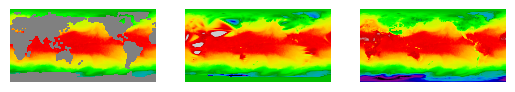
Figure 6: Land regions are masked which is motivated by situations when observations are only available for the sea surface (left). In order to adopt FNO to masked input tasks, we incorporated interpolated values (middle). However, there can be a large gap between the real temperature field (right) and the interpolated inputs.

Additional results

Long-term predictions

We conducted experiments with extended long-term predictions with IPOT and DINO (Yin et al. 2022) (state-of-the-art comparison) in Table 7. The original test set from (Yin et al. 2022) consists of long trajectories (160 frames) each of which is divided into 8 short trajectories (20 frames). We modified the slicing scheme so that each long trajectory is divided into 4 short trajectories (40 frames). Table 7 includes extended predictions on both approaches on $t=20-30$ and $t=30-40$. The result supports our model’s stability in producing accurate long-term predictions. Also, we provide the visualization of predictions of IPOT on $t=0,10,20,30$, and $40$ in Figure 4 (left) in the main text.

Table 7: Long-term predictions of DINO and IPOT on spherical shallow water.

Model	Shallow water
	$t$=0-10	$t$=10-20	$t$=20-30	$t$=30-40
DINO	1.06e–4	6.47e–4	1.37e–3	1.52e–03
IPOT	1.74e–4	5.12e–4	1.00e–3	1.11e–03

Compared with Perceiver IO

We conducted experiments with long-term predictions with IPOT and perceiver io (Jaegle et al. 2022) in Table 8.

Table 8: Performance comparisons with Perceiver IO on Navier-Stokes equations.

Model	Navier Stokes
	$\nu$=1e–3	$\nu$=1e–4	$\nu$=1e–5
Perceiver IO	1.83e–2	2.59e–1	2.76e–1
IPOT	8.85e–3	1.22e–1	1.48e–1

References

- Ba, Kiros, and Hinton (2016) Ba, J. L.; Kiros, J. R.; and Hinton, G. E. 2016. Layer normalization. arXiv preprint arXiv:1607.06450.
- Belbute-Peres, Economon, and Kolter (2020) Belbute-Peres, F. D. A.; Economon, T.; and Kolter, Z. 2020. Combining differentiable PDE solvers and graph neural networks for fluid flow prediction. In international conference on machine learning, 2402–2411. PMLR.
- Bode et al. (2021) Bode, M.; Gauding, M.; Lian, Z.; Denker, D.; Davidovic, M.; Kleinheinz, K.; Jitsev, J.; and Pitsch, H. 2021. Using physics-informed enhanced super-resolution generative adversarial networks for subfilter modeling in turbulent reactive flows. Proceedings of the Combustion Institute, 38(2): 2617–2625.
- Brandstetter, Worrall, and Welling (2022) Brandstetter, J.; Worrall, D. E.; and Welling, M. 2022. Message Passing Neural PDE Solvers. In International Conference on Learning Representations.
- Brenner, Scott, and Scott (2008) Brenner, S. C.; Scott, L. R.; and Scott, L. R. 2008. The mathematical theory of finite element methods, volume 3. Springer.
- Cao (2021) Cao, S. 2021. Choose a transformer: Fourier or galerkin. Advances in Neural Information Processing Systems, 34.
- Cao et al. (2013) Cao, Y.; Brubaker, M. A.; Fleet, D. J.; and Hertzmann, A. 2013. Efficient optimization for sparse Gaussian process regression. Advances in Neural Information Processing Systems, 26.
- Chen and Chen (1995) Chen, T.; and Chen, H. 1995. Universal approximation to nonlinear operators by neural networks with arbitrary activation functions and its application to dynamical systems. IEEE Transactions on Neural Networks, 6(4): 911–917.
- Choromanski et al. (2021) Choromanski, K. M.; Likhosherstov, V.; Dohan, D.; Song, X.; Gane, A.; Sarlos, T.; Hawkins, P.; Davis, J. Q.; Mohiuddin, A.; Kaiser, L.; Belanger, D. B.; Colwell, L. J.; and Weller, A. 2021. Rethinking Attention with Performers. In International Conference on Learning Representations.
- Galewsky, Scott, and Polvani (2004) Galewsky, J.; Scott, R. K.; and Polvani, L. M. 2004. An initial-value problem for testing numerical models of the global shallow-water equations. Tellus A: Dynamic Meteorology and Oceanography, 56(5): 429–440.
- Guibas et al. (2021) Guibas, J.; Mardani, M.; Li, Z.; Tao, A.; Anandkumar, A.; and Catanzaro, B. 2021. Adaptive Fourier Neural Operators: Efficient Token Mixers for Transformers. arXiv preprint arXiv:2111.13587.
- Guo, Cao, and Chen (2023) Guo, R.; Cao, S.; and Chen, L. 2023. Transformer Meets Boundary Value Inverse Problems. In The Eleventh International Conference on Learning Representations.
- Gupta, Xiao, and Bogdan (2021) Gupta, G.; Xiao, X.; and Bogdan, P. 2021. Multiwavelet-based Operator Learning for Differential Equations. In Beygelzimer, A.; Dauphin, Y.; Liang, P.; and Vaughan, J. W., eds., Advances in Neural Information Processing Systems.
- Ha, Dai, and Le (2016) Ha, D.; Dai, A.; and Le, Q. V. 2016. Hypernetworks. arXiv preprint arXiv:1609.09106.
- Hao et al. (2023) Hao, Z.; Ying, C.; Wang, Z.; Su, H.; Dong, Y.; Liu, S.; Cheng, Z.; Zhu, J.; and Song, J. 2023. GNOT: A General Neural Operator Transformer for Operator Learning. arXiv preprint arXiv:2302.14376.
- He and Xu (2019) He, J.; and Xu, J. 2019. MgNet: A unified framework of multigrid and convolutional neural network. Science china mathematics, 62: 1331–1354.
- Hendrycks and Gimpel (2016) Hendrycks, D.; and Gimpel, K. 2016. Gaussian error linear units (gelus). arXiv preprint arXiv:1606.08415.
- Hersbach et al. (2020) Hersbach, H.; Bell, B.; Berrisford, P.; Hirahara, S.; Horányi, A.; Muñoz-Sabater, J.; Nicolas, J.; Peubey, C.; Radu, R.; Schepers, D.; et al. 2020. The ERA5 global reanalysis. Quarterly Journal of the Royal Meteorological Society, 146(730): 1999–2049.
- Huang and Russell (2010) Huang, W.; and Russell, R. D. 2010. Adaptive moving mesh methods, volume 174. Springer Science & Business Media.
- Jaegle et al. (2022) Jaegle, A.; Borgeaud, S.; Alayrac, J.-B.; Doersch, C.; Ionescu, C.; Ding, D.; Koppula, S.; Zoran, D.; Brock, A.; Shelhamer, E.; Henaff, O. J.; Botvinick, M.; Zisserman, A.; Vinyals, O.; and Carreira, J. 2022. Perceiver IO: A General Architecture for Structured Inputs & Outputs. In International Conference on Learning Representations.
- Jaegle et al. (2021) Jaegle, A.; Gimeno, F.; Brock, A.; Vinyals, O.; Zisserman, A.; and Carreira, J. 2021. Perceiver: General perception with iterative attention. In International Conference on Machine Learning, 4651–4664. PMLR.
- Jiang et al. (2020) Jiang, C. M.; Esmaeilzadeh, S.; Azizzadenesheli, K.; Kashinath, K.; Mustafa, M.; Tchelepi, H. A.; Marcus, P.; Prabhat; and Anandkumar, A. 2020. MeshfreeFlowNet: A Physics-Constrained Deep Continuous Space-Time Super-Resolution Framework. In Proceedings of the International Conference for High Performance Computing, Networking, Storage and Analysis.
- Karniadakis et al. (2021) Karniadakis, G. E.; Kevrekidis, I. G.; Lu, L.; Perdikaris, P.; Wang, S.; and Yang, L. 2021. Physics-informed machine learning. Nature Reviews Physics, 3(6): 422–440.
- Kashefi and Mukerji (2022) Kashefi, A.; and Mukerji, T. 2022. Physics-Informed PointNet: A Deep Learning Solver for Steady-State Incompressible Flows and Thermal Fields on Multiple Sets of Irregular Geometries. J. Comput. Phys., 468.
- Kashefi, Rempe, and Guibas (2021) Kashefi, A.; Rempe, D.; and Guibas, L. J. 2021. A point-cloud deep learning framework for prediction of fluid flow fields on irregular geometries. Physics of Fluids, 33(2): 027104.
- Kovachki et al. (2021) Kovachki, N.; Li, Z.; Liu, B.; Azizzadenesheli, K.; Bhattacharya, K.; Stuart, A.; and Anandkumar, A. 2021. Neural operator: Learning maps between function spaces. arXiv preprint arXiv:2108.08481.
- Lee et al. (2019) Lee, J.; Lee, Y.; Kim, J.; Kosiorek, A.; Choi, S.; and Teh, Y. W. 2019. Set transformer: A framework for attention-based permutation-invariant neural networks. In International Conference on Machine Learning, 3744–3753. PMLR.
- Lee (2022) Lee, S. 2022. Mesh-Independent Operator Learning for Partial Differential Equations. In ICML 2022 2nd AI for Science Workshop.
- Li et al. (2022) Li, Z.; Huang, D. Z.; Liu, B.; and Anandkumar, A. 2022. Fourier neural operator with learned deformations for pdes on general geometries. arXiv preprint arXiv:2207.05209.
- Li et al. (2020a) Li, Z.; Kovachki, N.; Azizzadenesheli, K.; Liu, B.; Bhattacharya, K.; Stuart, A.; and Anandkumar, A. 2020a. Neural operator: Graph kernel network for partial differential equations. arXiv preprint arXiv:2003.03485.
- Li et al. (2021a) Li, Z.; Kovachki, N.; Azizzadenesheli, K.; Liu, B.; Bhattacharya, K.; Stuart, A.; and Anandkumar, A. 2021a. Markov neural operators for learning chaotic systems. arXiv preprint arXiv:2106.06898.
- Li et al. (2020b) Li, Z.; Kovachki, N.; Azizzadenesheli, K.; Liu, B.; Stuart, A.; Bhattacharya, K.; and Anandkumar, A. 2020b. Multipole graph neural operator for parametric partial differential equations. Advances in Neural Information Processing Systems, 33: 6755–6766.
- Li et al. (2021b) Li, Z.; Kovachki, N. B.; Azizzadenesheli, K.; liu, B.; Bhattacharya, K.; Stuart, A.; and Anandkumar, A. 2021b. Fourier Neural Operator for Parametric Partial Differential Equations. In International Conference on Learning Representations.
- Li, Meidani, and Farimani (2022) Li, Z.; Meidani, K.; and Farimani, A. B. 2022. Transformer for partial differential equations’ operator learning. arXiv preprint arXiv:2205.13671.
- Lienen and Günnemann (2022) Lienen, M.; and Günnemann, S. 2022. Learning the Dynamics of Physical Systems from Sparse Observations with Finite Element Networks. In International Conference on Learning Representations.
- Liu, Xu, and Zhang (2022) Liu, X.; Xu, B.; and Zhang, L. 2022. HT-Net: Hierarchical Transformer based Operator Learning Model for Multiscale PDEs. arXiv preprint arXiv:2210.10890.
- Loshchilov and Hutter (2019) Loshchilov, I.; and Hutter, F. 2019. Decoupled Weight Decay Regularization. In International Conference on Learning Representations.
- Lu, Jin, and Karniadakis (2019) Lu, L.; Jin, P.; and Karniadakis, G. E. 2019. Deeponet: Learning nonlinear operators for identifying differential equations based on the universal approximation theorem of operators. arXiv preprint arXiv:1910.03193.
- Lu et al. (2021) Lu, L.; Jin, P.; Pang, G.; Zhang, Z.; and Karniadakis, G. E. 2021. Learning nonlinear operators via DeepONet based on the universal approximation theorem of operators. Nature Machine Intelligence, 3(3): 218–229.
- Lu et al. (2022) Lu, L.; Meng, X.; Cai, S.; Mao, Z.; Goswami, S.; Zhang, Z.; and Karniadakis, G. E. 2022. A comprehensive and fair comparison of two neural operators (with practical extensions) based on fair data. Computer Methods in Applied Mechanics and Engineering, 393: 114778.
- Mildenhall et al. (2020) Mildenhall, B.; Srinivasan, P. P.; Tancik, M.; Barron, J. T.; Ramamoorthi, R.; and Ng, R. 2020. Nerf: Representing scenes as neural radiance fields for view synthesis. In European conference on computer vision, 405–421. Springer.
- Nguyen, Chen, and Lee (2021) Nguyen, T.; Chen, Z.; and Lee, J. 2021. Dataset Meta-Learning from Kernel Ridge-Regression. In International Conference on Learning Representations.
- Pan, Brunton, and Kutz (2022) Pan, S.; Brunton, S. L.; and Kutz, J. N. 2022. Neural Implicit Flow: a mesh-agnostic dimensionality reduction paradigm of spatio-temporal data. arXiv preprint arXiv:2204.03216.
- Pathak et al. (2022) Pathak, J.; Subramanian, S.; Harrington, P.; Raja, S.; Chattopadhyay, A.; Mardani, M.; Kurth, T.; Hall, D.; Li, Z.; Azizzadenesheli, K.; et al. 2022. FourCastNet: A Global Data-driven High-resolution Weather Model using Adaptive Fourier Neural Operators. arXiv preprint arXiv:2202.11214.
- Pfaff et al. (2021) Pfaff, T.; Fortunato, M.; Sanchez-Gonzalez, A.; and Battaglia, P. 2021. Learning Mesh-Based Simulation with Graph Networks. In International Conference on Learning Representations.
- Qi et al. (2017) Qi, C. R.; Su, H.; Mo, K.; and Guibas, L. J. 2017. Pointnet: Deep learning on point sets for 3d classification and segmentation. In Proceedings of the IEEE conference on computer vision and pattern recognition, 652–660.
- Quiñonero-Candela and Rasmussen (2005) Quiñonero-Candela, J.; and Rasmussen, C. E. 2005. A Unifying View of Sparse Approximate Gaussian Process Regression. Journal of Machine Learning Research, 6(65): 1939–1959.
- Raissi, Perdikaris, and Karniadakis (2019) Raissi, M.; Perdikaris, P.; and Karniadakis, G. E. 2019. Physics-informed neural networks: A deep learning framework for solving forward and inverse problems involving nonlinear partial differential equations. Journal of Computational physics, 378: 686–707.
- Rastogi et al. (2023) Rastogi, R.; Schiff, Y.; Hacohen, A.; Li, Z.; Lee, I.; Deng, Y.; Sabuncu, M. R.; and Kuleshov, V. 2023. Semi-Parametric Inducing Point Networks and Neural Processes. In The Eleventh International Conference on Learning Representations.
- Sanchez-Gonzalez et al. (2020) Sanchez-Gonzalez, A.; Godwin, J.; Pfaff, T.; Ying, R.; Leskovec, J.; and Battaglia, P. 2020. Learning to simulate complex physics with graph networks. In International conference on machine learning, 8459–8468. PMLR.
- Sitzmann et al. (2020) Sitzmann, V.; Martel, J.; Bergman, A.; Lindell, D.; and Wetzstein, G. 2020. Implicit neural representations with periodic activation functions. Advances in Neural Information Processing Systems, 33.
- Snelson and Ghahramani (2005) Snelson, E.; and Ghahramani, Z. 2005. Sparse Gaussian Processes using Pseudo-inputs. In Weiss, Y.; Schölkopf, B.; and Platt, J., eds., Advances in Neural Information Processing Systems, volume 18. MIT Press.
- Strauss (2007) Strauss, W. A. 2007. Partial differential equations: An introduction. John Wiley & Sons.
- Tancik et al. (2020) Tancik, M.; Srinivasan, P.; Mildenhall, B.; Fridovich-Keil, S.; Raghavan, N.; Singhal, U.; Ramamoorthi, R.; Barron, J.; and Ng, R. 2020. Fourier features let networks learn high frequency functions in low dimensional domains. Advances in Neural Information Processing Systems, 33.
- Tang and Ha (2021) Tang, Y.; and Ha, D. 2021. The sensory neuron as a transformer: Permutation-invariant neural networks for reinforcement learning. Advances in Neural Information Processing Systems, 34.
- Titsias (2009) Titsias, M. 2009. Variational Learning of Inducing Variables in Sparse Gaussian Processes. In van Dyk, D.; and Welling, M., eds., Proceedings of the Twelth International Conference on Artificial Intelligence and Statistics, volume 5 of Proceedings of Machine Learning Research, 567–574. Hilton Clearwater Beach Resort, Clearwater Beach, Florida USA: PMLR.
- Tran et al. (2023) Tran, A.; Mathews, A.; Xie, L.; and Ong, C. S. 2023. Factorized Fourier Neural Operators. In The Eleventh International Conference on Learning Representations.
- Tripura and Chakraborty (2023) Tripura, T.; and Chakraborty, S. 2023. Wavelet Neural Operator for solving parametric partial differential equations in computational mechanics problems. Computer Methods in Applied Mechanics and Engineering, 404: 115783.
- Tsai et al. (2019) Tsai, Y.-H. H.; Bai, S.; Yamada, M.; Morency, L.-P.; and Salakhutdinov, R. 2019. Transformer Dissection: A Unified Understanding of Transformer’s Attention via the Lens of Kernel. arXiv preprint arXiv:1908.11775.
- Vaswani et al. (2017) Vaswani, A.; Shazeer, N.; Parmar, N.; Uszkoreit, J.; Jones, L.; Gomez, A. N.; Kaiser, Ł.; and Polosukhin, I. 2017. Attention is all you need. Advances in neural information processing systems, 30.
- Xiong et al. (2021) Xiong, Y.; Zeng, Z.; Chakraborty, R.; Tan, M.; Fung, G.; Li, Y.; and Singh, V. 2021. Nyströmformer: A Nystöm-based Algorithm for Approximating Self-Attention. In Proceedings of the… AAAI Conference on Artificial Intelligence. AAAI Conference on Artificial Intelligence, volume 35, 14138. NIH Public Access.
- Yin et al. (2022) Yin, Y.; Kirchmeyer, M.; Franceschi, J.-Y.; Rakotomamonjy, A.; and Gallinari, P. 2022. Continuous PDE Dynamics Forecasting with Implicit Neural Representations. arXiv preprint arXiv:2209.14855.