Robust Node Representation Learning via Graph Variational Diffusion Networks

Abstract

Node representation learning by using Graph Neural Networks (GNNs) has been widely explored. However, in recent years, compelling evidence has revealed that GNN-based node representation learning can be substantially deteriorated by delicately-crafted perturbations in a graph structure. To learn robust node representation in the presence of perturbations, various works have been proposed to safeguard GNNs. Within these existing works, Bayesian label transition has been proven to be more effective, but this method is extensively reliant on a well-built prior distribution. The variational inference could address this limitation by sampling the latent node embedding from a Gaussian prior distribution. Besides, leveraging the Gaussian distribution (noise) in hidden layers is an appealing strategy to strengthen the robustness of GNNs. However, our experiments indicate that such a strategy can cause over-smoothing issues during node aggregation. In this work, we propose the Graph Variational Diffusion Network (GVDN), a new node encoder that effectively manipulates Gaussian noise to safeguard robustness on perturbed graphs while alleviating over-smoothing issues through two mechanisms: Gaussian diffusion and node embedding propagation. Thanks to these two mechanisms, our model can generate robust node embeddings for recovery. Specifically, we design a retraining mechanism using the generated node embedding to recover the performance of node classifications in the presence of perturbations. The experiments verify the effectiveness of our proposed model across six public datasets.

Introduction

Various web data can be represented as attributed graphs, such as citation networks (Sen et al. 2008), co-purchase networks (Shchur et al. 2018), and online social networks (OSNs) (Hamilton, Ying, and Leskovec 2017); the entities in these networks can be characterized as vertices, whereas the relationship between two entities can be depicted as a link. As a powerful Artificial Intelligence (AI) technique for learning node representations in attributed graphs, Graph Neural Networks (GNNs) (Bruna et al. 2013; Defferrard, Bresson, and Vandergheynst 2016; Kipf and Welling 2016a) are widely explored in numerous scenarios, such as user profiling in OSNs (Chen et al. 2019; Zhuang and Hasan 2022), community detection (Breuer, Eilat, and Weinsberg 2020), community-based question answering (Fang et al. 2016), recommendation systems (Ying et al. 2018), etc. A capstone of GNNs is the message-passing mechanism, which propagates the topology-based hidden representation by aggregating the node and features layer by layer. In recent years, however, compelling evidence reveals that this mechanism may substantially deteriorate by delicately-crafted perturbations in a graph structure (Sun et al. 2018a; Jin et al. 2020a), raising concerns about the reliability and robustness of GNNs. For instance, in OSNs, non-malicious users may randomly connect with many other users for business promotion purposes (Zhuang and Al Hasan 2022b). On the other extreme, the message-passing mechanism may perform poorly on new OSN users who lack sufficient connections with other users (edges) or profile information (feature) (Tam and Dunson 2020; Ye and Ji 2021). Third, adversarial attacks may significantly deteriorate the performance of GNNs with unnoticeable modification of graphs (Zügner, Akbarnejad, and Günnemann 2018; Dai et al. 2018).

Many recent works have been proposed to learn robust node representation against the above-mentioned perturbations. We categorize these works from the perspective of processing stages as follows. Topological denoising methods (Wu et al. 2019b; Entezari et al. 2020; Rong et al. 2019) preprocess the poisoned graphs by eliminating suspicious edges before node aggregation in the pre-processing stage. However, these kinds of methods may fail to prune suspicious edges when the graph structure is sparse. Mechanism design methods generally propose mechanisms, such as node aggregators (Feng et al. 2020; Jin et al. 2021), and regularization (Chang et al. 2021; Liu et al. 2021), to strengthen the robustness of node classifications in the inter-processing stage. Nevertheless, these methods heavily rely on heuristic explorations of topological structures of graphs and may perform worse under severe perturbations. Bayesian label transition methods (Zhuang and Al Hasan 2022b, a) tackle the perturbation issues in the post-processing stage by aligning the inferred labels to the original labels as closely as possible through MCMC-based sampling. The post-processing inference is proved to yield better accuracy on perturbed graphs, but this inference highly depends on the quality of predictions on the training data because MCMC methods indirectly sample the labels from the prior distribution, which is built on the training set (Van Ravenzwaaij, Cassey, and Brown 2018). Such a limitation could be addressed by variational inference (Kingma and Welling 2013) that samples from a robust prior distribution, e.g., Gaussian distribution, which is parameterized by mean $\mu$ and standard deviation $\sigma$. Besides, leveraging the Gaussian distribution, a.k.a. Gaussian noise, to strengthen the robustness of GNNs is an appealing strategy (Zhu et al. 2019; Godwin et al. 2021; Bo et al. 2021). To verify the effectiveness of this strategy, we conduct ablation experiments by adjusting the weight of Gaussian noise in the hidden layers of GNNs. The results suggest that simply increasing the percentage of Gaussian noise in the hidden layers tends to deteriorate the node classification accuracy. We argue that injecting Gaussian noise indiscriminately would cause over-smoothing issues in node aggregation. Based on this hypothesis, we face a core challenge: How to take advantage of Gaussian noise to enhance robustness against perturbations while simultaneously alleviating over-smoothing issues?

To embrace this challenge, we propose the Graph Variational Diffusion Network (GVDN), a novel node encoder that dynamically regulates the magnitude of noise and further safeguards robustness via two mechanisms: Gaussian diffusion and node embedding propagation. The first mechanism draws inspiration from variational diffusion models, which are commonly used in image synthesis (Ho, Jain, and Abbeel 2020). The motivation for Gaussian diffusion is that the strategy of leveraging Gaussian noise may require less help from the noise as training progresses (the model becomes stronger). Gaussian diffusion linearly decreases the extent of Gaussian noise at each successive iteration to help train a robust model. Our experiments unearth that applying diffusion to $\mu$ and $\sigma$ before variational sampling via reparameterization can affirmatively help generalize the robustness of recovery on perturbed graphs. The second mechanism is motivated by a recent study (Zhuang and Al Hasan 2022c), which empirically verifies that label propagation can alleviate node vulnerability. Such propagation is based on the assumption of the graph homophily property (Zhu et al. 2020) that adjacent vertices tend to have similar class labels. Experiments indicate that propagating adjacent node embeddings of inaccurately predicted nodes, whose adjacent neighbors are selected by a topology-based sampler, during training can further strengthen the robustness.

Owing to the two mechanisms, our model can generate robust node embedding for downstream tasks. One benefit is that in real-world web applications, node embedding can be generated by an offline-trained GNN and further used for online downstream tasks, such as recommendation (Sun et al. 2018b) or search (Xiong, Power, and Callan 2017). In this study, our downstream task is to recover the performance of node classifications on perturbed graphs; specifically, we design a retraining mechanism to recover the performance by retraining the GNN-based node classifier on perturbed graphs using the previously generated node embedding. One advantage of our model over MCMC methods, such as GraphSS (Zhuang and Al Hasan 2022a), is that our model doesn’t require a well-built prior distribution from the training data. Besides, the experiments verify that our proposed retraining mechanism outperforms all competing methods in accuracy on perturbed graphs across all datasets. Overall, our contributions can be summarized as follows:

• We propose a new node encoder, namely the Graph Variational Diffusion Network (GVDN), to generate node embedding for robust node representation learning. To the best of our knowledge, our work is the first model that leverages variational diffusion with node embedding propagation to safeguard robustness against perturbations while alleviating over-smoothing issues on GNNs.

• We design a retraining mechanism using the generated node embedding to recover the performance of node classifications on perturbed graphs. Experiments validate the effectiveness of our model across six public datasets.

Methodology

In this section, we first briefly introduce the notations. Most importantly, we introduce our proposed model in detail from the perspectives of frameworks, optimization, training procedure, retraining mechanism, and time complexity.

Notations. We denote an undirected attributed graph as $\mathcal{G}$, which consists of a set of vertices $\mathcal{V}$ = $\{v_{1},v_{2},...,v_{N}\}$ and edges $\mathcal{E}\subseteq\mathcal{V}\times\mathcal{V}$, where $N$ is the number of vertices in $\mathcal{G}$. The topological relationship among vertices can be represented by a symmetric adjacency matrix $\mathbf{A}\in\mathbb{R}^{N\times N}$. We preprocess the adjacency matrix as follows:

$$\mathbf{\hat{A}}=\mathbf{\tilde{D}}^{-\frac{1}{2}}\mathbf{\tilde{A}}\mathbf{\tilde{D}}^{-\frac{1}{2}},$$ (1)

where $\mathbf{\tilde{A}}=\mathbf{A}+I_{N}$, $\mathbf{\tilde{D}}=\mathbf{D}+I_{N}$. $I_{N}$ is an identity matrix. $\mathbf{D}_{i,i}=\sum_{j}\mathbf{A}_{i,j}$ is a diagonal degree matrix.

In an attributed graph, each vertex contains a feature vector. All feature vectors constitute a feature matrix $\mathbf{X}\in\mathbb{R}^{N\times d}$, where $d$ is the number of features for each vertex. Given $\mathbf{\hat{A}}$ and $\mathbf{X}$, a layer-wise message-passing mechanism of GNNs can be formulated as follows:

$$\textit{f}_{\mathbf{W}^{(l)}}\left(\mathbf{\hat{A}},\mathbf{H}^{(l)}\right)=\mathbf{\hat{A}}\mathbf{H}^{(l)}\mathbf{W}^{(l)},$$ (2)

where $\mathbf{H}^{(l)}$ is a node hidden representation in the $l$-th layer. The dimension of $\mathbf{H}^{(l)}$ in the input layer, middle layer, and output layer is the number of features $d$, hidden units $h$, and classes $K$, respectively. $\mathbf{H}^{(0)}=\mathbf{X}$. $\mathbf{W}^{(l)}$ is the weight matrix in the $l$-th layer.

In this work, we aim to develop a node encoder to generate robust node embedding, a.k.a. node hidden representation, for the downstream node classification task on perturbed graphs. In general node classification tasks, a GNN takes both $\mathbf{\hat{A}}$ and $\mathbf{X}$ as inputs and is trained with ground-truth labels $\mathbf{Y}\in\mathbb{R}^{N\times 1}$. Besides, we denote the predicted labels as $\mathbf{\hat{Y}}\in\mathbb{R}^{N\times 1}$ (pronounced as ”Y hat”) and the sampled labels as $\mathbf{\bar{Y}}\in\mathbb{R}^{N\times 1}$ (pronounced as ”Y bar”). We formally state the problem that we aim to address as follows:

Problem 1

Given a graph $\mathcal{G}=(\mathbf{\hat{A}},\mathbf{X})$ and the ground-truth labels $\mathbf{Y}$, we train our proposed node encoder on unperturbed $\mathcal{G}_{train}$ to generate node embedding for recovering the node classification performance of the GNN on perturbed $\mathcal{G}_{test}$.

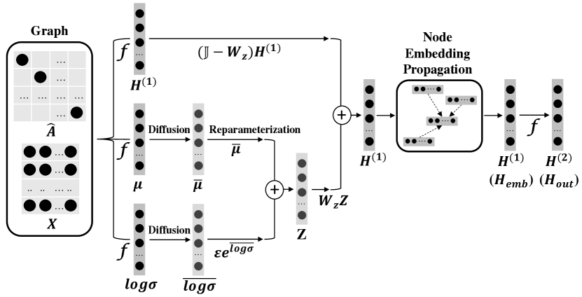
Figure 1: The overall framework of our proposed model. Given a preprocessed adjacency matrix $\mathbf{\hat{A}}$ and a feature matrix $\mathbf{X}$, we first generate the first-layer node hidden representation $\mathbf{H}^{(1)}$, mean matrix $\mathbf{\mu}$, and log standard deviation matrix $\mathbf{log\sigma}$ by node aggregation $f$ with RELU activation function in this layer. Then, we apply Gaussian diffusion to get diffused $\overline{\mu}$ and $\overline{log\sigma}$. Furthermore, we sample the posterior $\mathbf{Z}$ by reparameterization, where $\epsilon\sim\mathcal{N}(0,I)$. After sampling, we add up two terms of element-wise multiplication, $\left(\mathbb{J}-\mathbf{W}_{z}\right)\mathbf{H}^{(1)}$ and $\mathbf{W}_{z}\mathbf{Z}$. During the training, we apply node embedding propagation to further strengthen robustness. In the end, we output the $\mathbf{H}^{(1)}$ as the node embedding $\mathbf{H}_{emb}$ and obtain the output node representation $\mathbf{H}_{out}$ by aggregating nodes to the second-layer node hidden representation $\mathbf{H}^{(2)}$. Note that the solid arrows denote the directions of the forward propagation, whereas the dashed arrows denote the node embedding propagation.

The Proposed Model. Variational sampling is widely used in variational graph auto-encoders to generate node representation for graph reconstructions (Kipf and Welling 2016b; Pan et al. 2018). We apply Gaussian diffusion to variational sampling along with node embedding propagation to mitigate the above issues in our model. The overall framework is briefly introduced in Fig. 1. Specifically, given a graph $\mathcal{G}$=$(\mathbf{\hat{A}},\mathbf{X})$, our model first generates the node hidden representation $\mathbf{H}^{(1)}$, the matrix of mean $\mu$, and the matrix of log standard deviation $log\sigma$ by Eq. 2 as follows:

$$\left\{\begin{array}[]{lr}\mathbf{H}^{(1)}=ReLU\left(\textit{f}_{\mathbf{W}_{h}^{(0)}}\left(\mathbf{\hat{A}},\mathbf{X}\right)\right),&\\ \mu=ReLU\left(\textit{f}_{\mathbf{W}_{\mu}}\left(\mathbf{\hat{A}},\mathbf{X}\right)\right),&\\ log\sigma=ReLU\left(\textit{f}_{\mathbf{W}_{\sigma}}\left(\mathbf{\hat{A}},\mathbf{X}\right)\right),\end{array}\right.$$ (3)

where $\mathbf{W}_{h}^{(0)}\in\mathbb{R}^{d\times h}$, $\mathbf{W}_{\mu}\in\mathbb{R}^{d\times h}$, and $\mathbf{W}_{\sigma}\in\mathbb{R}^{d\times h}$ represent the corresponding weight matrix for $\mathbf{H}^{(1)}$, $\mu$, and $log\sigma$. $ReLU(\cdot)$ is a non-linear activation function.

Inspired by the variational diffusion models (Ho, Jain, and Abbeel 2020; Kingma et al. 2021), we apply Gaussian diffusion to the $\mu$ and $log\sigma$ matrices with the decreasing diffusion rate $\gamma$ as follows:

$$\left\{\begin{array}[]{lr}\overline{\mu}=\sqrt{\Gamma_{t}}\mu,&\\ \overline{log\sigma}=\sqrt{(1-\Gamma_{t})}log\sigma,\end{array}\right.$$ (4)

where $\overline{\mu}$ and $\overline{log\sigma}$ are denoted as the diffused $\mu$ and $log\sigma$, respectively; $\Gamma_{t}=\prod_{i=1}^{t}\gamma_{i}$ is the accumulated production of previous diffusion rates in the $t$-th iteration. The $\gamma$ linearly decreases with each iteration. Such a decrease simulates the process that a drop of ink spreads on the water.

To ensure that the gradient can be back-propagated, we sample the node hidden representation $\mathbf{Z}$ from $\overline{\mu}$ and $\overline{log\sigma}$ using a reparameterization trick.

$$\mathbf{Z}=\overline{\mu}+\epsilon e^{\overline{log\sigma}},\ \ \epsilon\sim\mathcal{N}(0,I).$$ (5)

After sampling, we add up two terms of element-wise multiplication, $\left(\mathbb{J}-\mathbf{W}_{z}\right)\mathbf{H}^{(1)}$ and $\mathbf{W}_{z}\mathbf{Z}$, where $\mathbb{J}\in\mathbb{R}^{|\mathbf{Z}|\times h}$ denotes the unit matrix (a.k.a. all-ones matrix) and the weight matrix $\mathbf{W}_{z}\in\mathbb{R}^{|\mathbf{Z}|\times h}$ can be automatically learned through back-propagation. Our experiments empirically verify that such an approach can mitigate the deterioration of GNNs that we presented in the ablation study.

$$\mathbf{H}^{(1)}=\left(\mathbb{J}-\mathbf{W}_{z}\right)\mathbf{H}^{(1)}+\mathbf{W}_{z}\mathbf{Z}.$$ (6)

To further strengthen robustness, we apply node embedding propagation during the training on inaccurately predicted nodes, whose neighbors are sampled in the preceding iteration. Algo. 1 presents the procedure by which we find the neighbors of the nodes with inaccurately predicted labels $\mathbf{\hat{Y}}^{t}$, s.t., $\mathbf{\hat{Y}}^{t}\neq\mathbf{Y}^{t}$, in the $t$-th iteration. To ascertain the neighbors of each inaccurately predicted node, we first sample a node label $\mathbf{\bar{y}}^{t}_{i}$ of the $i$-th node $v_{i}$ using a topology-based label sampler (line 3) and then select the neighbors with the same label of $\mathbf{\bar{y}}^{t}_{i}$ (line 4).

Algorithm 1 Topology-based sampling for selecting neighbors of inaccurate nodes in the $t$-th iteration.

Input: Predicted labels $\mathbf{\hat{Y}}^{t}$, The number of train nodes $N_{tr}$, Topology-based label sampler.

1:  for $i\leftarrow 0$ to $N_{tr}$ do

2:     if $\mathbf{\hat{y}}^{t}_{i}$ is inaccurate then

3:        Sample $\mathbf{\bar{y}}^{t}_{i}$ with the topology-based label sampler;

4:        Select the neighbors of $v_{i}$ based on $\mathbf{\bar{y}}^{t}_{i}$.

5:     end if

6:  end for

In the next iteration, for each inaccurately predicted node, we compute the mean matrix of the node embedding from its selected neighbors and then replace the node embedding of this node with the mean matrix. The benefit is that training the model with the propagated node embedding can effectively mitigate the vulnerability of these inaccurate nodes.

In the end, our model outputs $\mathbf{H}^{(1)}$ as the node embedding $\mathbf{H}_{emb}$ and $\mathbf{H}^{(2)}$ as the output node representation $\mathbf{H}_{out}$ for the downstream node classification. We compute $\mathbf{H}^{(2)}$ by:

$$\mathbf{H}^{(2)}=\textit{f}_{\mathbf{W}_{h}^{(1)}}\left(\mathbf{\hat{A}},\mathbf{H}^{(1)}\right),$$ (7)

where $\mathbf{W}_{h}^{(1)}\in\mathbb{R}^{h\times K}$ denotes the weight matrix for $\mathbf{H}_{out}$.

Optimization. We optimize our model with the following loss functions. First, we compute the cross entropy between predicted labels and ground-truth labels in the train graph.

$$\mathcal{L}_{ce}=-\frac{1}{N_{tr}}\sum_{i=1}^{N_{tr}}\sum_{k=1}^{K}y_{i,k}log(\hat{y}_{i,k}),$$ (8)

where $y_{i,k}$ denotes a ground-truth label of the $i$-th node in the $k$-th class; $\hat{y}_{i,k}$ denotes a predicted label of the $i$-th node in the $k$-th class; $N_{tr}$ denotes the number of train nodes; $K$ denotes the number of classes. In this work, we compute the $i$-th predicted label $\hat{y}_{i}$ by selecting the maximum probability of the corresponding categorical distribution, which is computed by employing a softmax function on the $i$-th $\mathbf{H}_{out}$.

To obtain the $\mu$ and $log\sigma$ for subsequent sampling, we apply the Kullback-Leibler divergence between the posterior distribution $\mathcal{Q}(\mu,\sigma^{2})$ before diffusion, where $\sigma=e^{log\sigma}$, and the prior distribution $\mathcal{N}(0,I)$ to ensure that these two distributions are as close as possible.

$$\mathcal{L}_{kl}=KL\left[\mathcal{Q}(\mu,\sigma^{2})\|\mathcal{N}(0,I)\right].$$ (9)

After applying diffusion by Eq. 4, we further match the sampled distribution $\mathbf{Z}\sim\mathcal{Q}(\overline{\mu},\overline{\sigma}^{2})$ with the Gaussian noise $\epsilon\sim\mathcal{N}(0,I)$ for preserving the Markovian property, where $\overline{\sigma}=e^{\overline{log\sigma}}$.

$$\mathcal{L}_{df}=\mathbb{E}\left[\|\epsilon-\mathbf{Z}\|^{2}\right].$$ (10)

During the retraining process, we match the predicted node embedding $\mathbf{\hat{H}}_{emb}$ (on the perturbed graphs) with the given pre-trained node embedding $\mathbf{H}_{emb}$ (on the unperturbed graphs) to enforce $\mathbf{\hat{H}}_{emb}$ as identically as $\mathbf{H}_{emb}$.

$$\mathcal{L}_{nm}=\mathbb{E}\left[\|\mathbf{H}_{emb}-\mathbf{\hat{H}}_{emb}\|^{2}\right].$$ (11)

Overall, we formulate the total objective function as:

$$\mathcal{L}_{GVDN}=\lambda^{T}\mathcal{L},$$ (12)

where $\mathcal{L}=[\mathcal{L}_{ce},\mathcal{L}_{kl},\mathcal{L}_{df},\mathcal{L}_{nm}]$ is a vector of losses; $\lambda^{T}\in\mathbb{R}^{|\mathcal{L}|\times 1}$ is a transposed vector of the balanced parameters, which is used for balancing the scale of each loss. Note that we only utilize the first three loss functions, $\mathcal{L}_{ce}$, $\mathcal{L}_{kl}$, and $\mathcal{L}_{df}$, during the training process and further include the last one, $\mathcal{L}_{nm}$, for retraining purposes.

Training. The procedure is summarized in Algo. 2. As an input, we use the ground-truth labels $\mathbf{Y}$ as the train labels during training, whereas, for retraining, we use the pseudo labels $\mathbf{\hat{Y}}_{pseudo}$. In each iteration, we compute losses, $\mathcal{L}_{ce}$, $\mathcal{L}_{kl}$, and $\mathcal{L}_{df}$ after the forward propagation during the training (line 2-5) and additionally compute the node-embedding matching loss $\mathcal{L}_{nm}$ for retraining purposes (line 6-7). Note that node embedding $\mathbf{H}_{emb}$ is used in both Eq. 11 and Algo. 3 during retraining. Besides, we select the neighbors of inaccurately predicted nodes with the topology-based sampler using Algo. 1 for node embedding propagation in the next iteration (line 9). At the end of each iteration, we apply backward propagation to compute the gradient (line 10) and then update all necessary weights (line 11). This procedure repeats $N_{epo}$ times until the loss has converged.

Algorithm 2 Training procedure of our model.

Input: Graph $\mathcal{G}_{train}=(\mathbf{\hat{A}}_{train},\mathbf{X}_{train})$, train labels, Node aggregator, Topology-based sampler, The number of training epochs $N_{epo}$.

1:  for $t\leftarrow 1$ to $N_{epo}$ do

2:     $\mathbf{H}_{out}\leftarrow$ Forward propagation;

3:     $\mathcal{L}_{ce}\leftarrow$ Compute the cross entropy loss by Eq. 8;

4:     $\mathcal{L}_{kl}\leftarrow$ Compute the KL-divergence by Eq. 9;

5:     $\mathcal{L}_{df}\leftarrow$ Compute the diffusion loss by Eq. 10;

6:     if Retraining then

7:        $\mathcal{L}_{nm}\leftarrow$ Compute the node-embedding matching loss by Eq. 11;

8:     end if

9:     Select the neighbors of inaccurately predicted nodes with the topology-based sampler by Algo. 1;

10:     Backward propagation using Eq. 12;

11:     Update the weights $\mathbf{W}_{h}^{(0)}$, $\mathbf{W}_{\mu}$, $\mathbf{W}_{\sigma}$, $\mathbf{W}_{z}$, and $\mathbf{W}_{h}^{(1)}$.

12:  end for

Algorithm 3 Retraining mechanism.

Input: A trained model, Node embedding $\mathbf{H}_{emb}$, Graph $\mathcal{G}_{pert}=(\mathbf{\hat{A}}_{pert},\mathbf{X}_{pert})$.

1:  $\mathbf{\hat{Y}}_{pseudo}=\mathop{\arg\max}\text{Softmax}\left(\textit{f}_{\mathbf{W}_{h}^{(1)}}\left(\mathbf{\hat{A}}_{pert},\mathbf{H}_{emb}\right)\right)$;

2:  Retrain the model with $\mathbf{\hat{Y}}_{pseudo}$ by Algo. 2.

Retraining Mechanism. In this work, we design a retraining mechanism for recovering the performance of the GNN on perturbed graphs. As presented in Algo. 3, we first generate pseudo labels $\mathbf{\hat{Y}}_{pseudo}$ using the given node embedding $\mathbf{H}_{emb}$ on perturbed graphs (line 1) and then retrain the model with $\mathbf{\hat{Y}}_{pseudo}$ by Algo. 2 (line 2). Overall, we train the model to generate robust node embedding $\mathbf{H}_{emb}$, which can be used for recovering the performance of GNNs on perturbed graphs via our retraining mechanism.

Time Complexity. During the training, we train our model with $N_{epo}$ epochs. For each epoch, our model traverses the number of train nodes $N_{tr}$ for forward and backward propagation. Besides, our model traverses the number of inaccurately predicted nodes $N_{ip}$ in the training nodes to sample the corresponding neighbors for node embedding propagation in the next iteration, where $N_{ip}\leq N_{tr}$. Thus, the node-level time complexity is $\mathcal{O}(N_{epo}\cdot N_{tr})$. To consider the time complexity at the element level, we can further multiply by $f_{l}$, where $f_{l}$ is the dimensionality of the $l^{th}$ hidden layer. So, the element-level time complexity is $\mathcal{O}(N_{epo}\cdot N_{tr}\cdot f_{l})$.

Experiments

In this section, we conduct ablation studies, generalization tests, comparison of competing methods, visualizations of node embeddings, analysis of convergence and parameters, and further discuss limitations and future directions.

Experimental Settings. We validate our model over six public graph datasets and follow the setting from (Zhuang and Al Hasan 2022c) to split the train, validation, and test graph to 10%, 20%, and 70% of the nodes, respectively. We compare our model with nine competing methods and evaluate the performance in accuracy (Acc.) and average normalized entropy (Ent.). Details are described in the Appendix.

Ablation Study. We conducted three experiments to examine our model architecture. First, we investigate how GNNs behave as the weight of the Gaussian noise $\mathbf{W}_{ns}$ (scalar) in the hidden layers increases and also compare the performance on Cora over four representative GNN models, including GCN (Kipf and Welling 2016a), GraphSAGE (Hamilton, Ying, and Leskovec 2017), SGC (Wu et al. 2019a), and GAT (Veličković et al. 2018), with our model. Specifically, we add standard Gaussian noise $\mathcal{N}(0,I)$ in the $l$-th hidden layer of four GNNs with the weight as follows:

$$\mathbf{H}^{(l)}=\left(1-\mathbf{W}_{ns}\right)\mathbf{H}^{(l)}+\mathbf{W}_{ns}\mathcal{N}(0,I).$$ (13)

We adjust the weights of four GNNs and present the trends in Fig. 2. The trends show that the accuracy decreases as the percentage of the weight increases and even drops dramatically when the percentage is higher than 90%. The normalized entropy has a similar pattern, which increases as the percentage of the weight increases.

$\bullet$ Observation: Simply increasing the percentage of the Gaussian noise in the hidden layer of GNNs by Eq. 13 will deteriorate the performance of node classifications, i.e., lead to lower accuracy and higher normalized entropy.

$\bullet$ Understanding: Node aggregation by Eq. 2 can be regarded as a kind of low-pass filtering (a.k.a. Gaussian filtering) because the message-passing mechanism aggregates the node features from local neighbors (Nt and Maehara 2019). Increasing the percentage of Gaussian noise in the hidden space tends to over-smooth the hidden representation and thus make node embeddings less distinct, which is well-known as an over-smoothing issue, i.e., distinct nodes have similar node embeddings in hidden spaces (Bo et al. 2021). This observation motivates us to explore a sophisticated approach that not only addresses over-smoothing issues but also leverages Gaussian noise against perturbation.

On the other hand, in the vanilla architecture of our model, we only concatenate both $\mathbf{H}^{(1)}$ and $\mathbf{Z}$ with the weight $\mathbf{W}_{z}$ by Eq. 6 without applying Gaussian diffusion and node embedding propagation. In our model, adjusting the weight of $\mathbf{Z}$ could be equivalent to changing the percentage of Gaussian noise in the hidden layers. The results in Fig. 2 show that our vanilla architecture can effectively maintain the performance, i.e., higher Acc. and lower Ent., as the percentage of the weight increases. This is possible since our model can learn the weight and adjust the values of noise to different nodes instead of assigning the same value to all nodes.

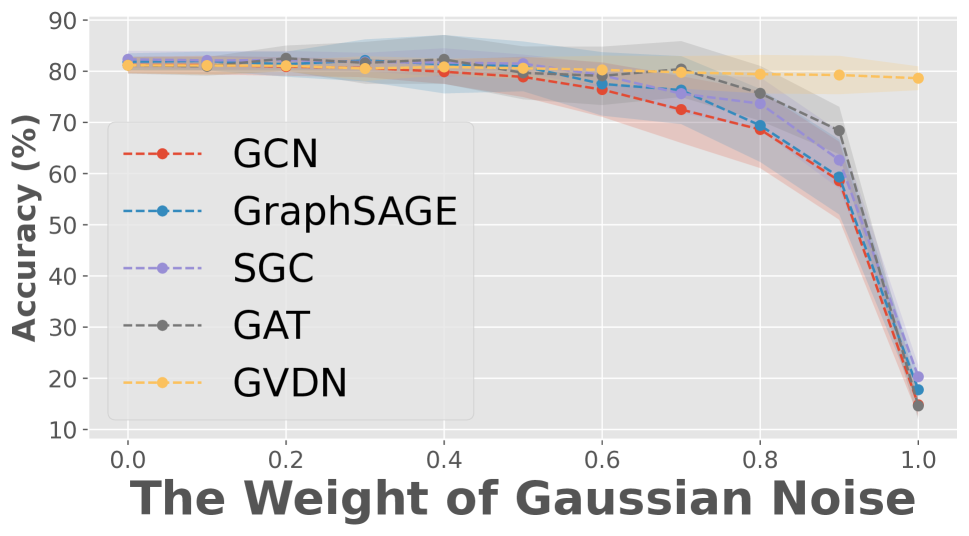
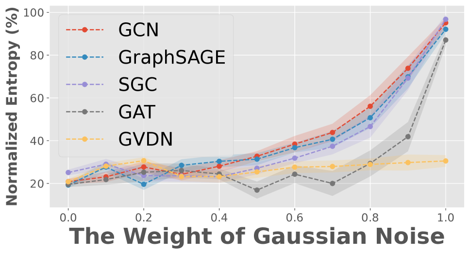
Figure 2: Verification of effectiveness on our vanilla model architecture by investigating how Gaussian noise affects the performance of the node classifications.

$p_{rdm}=1\%$ $p_{rdm}=5\%$

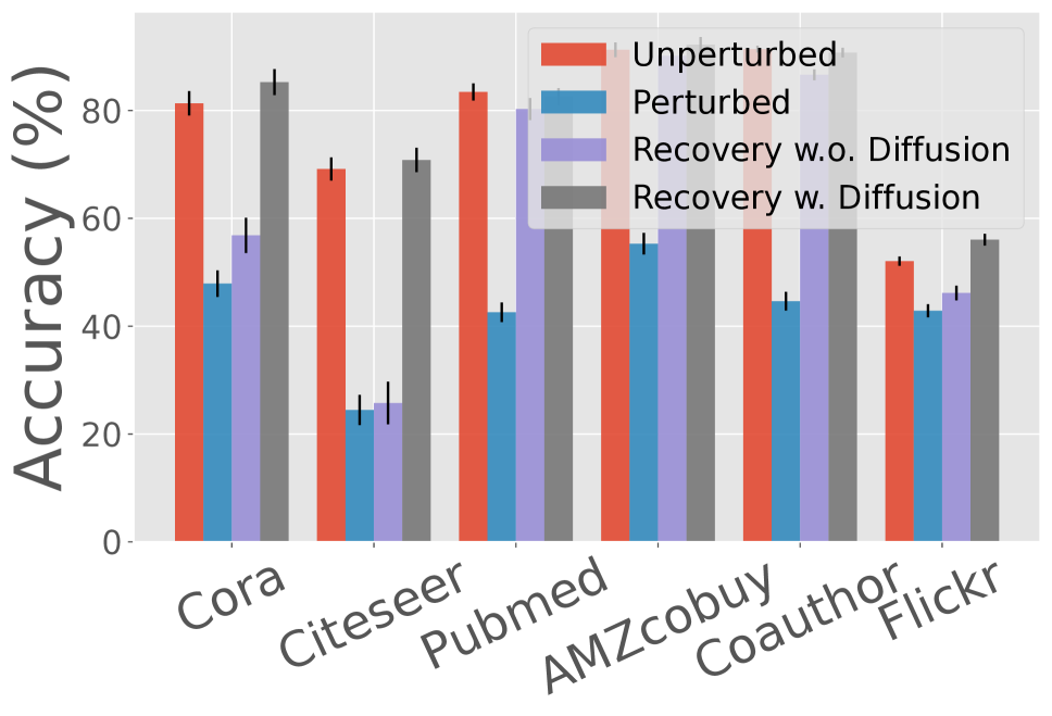
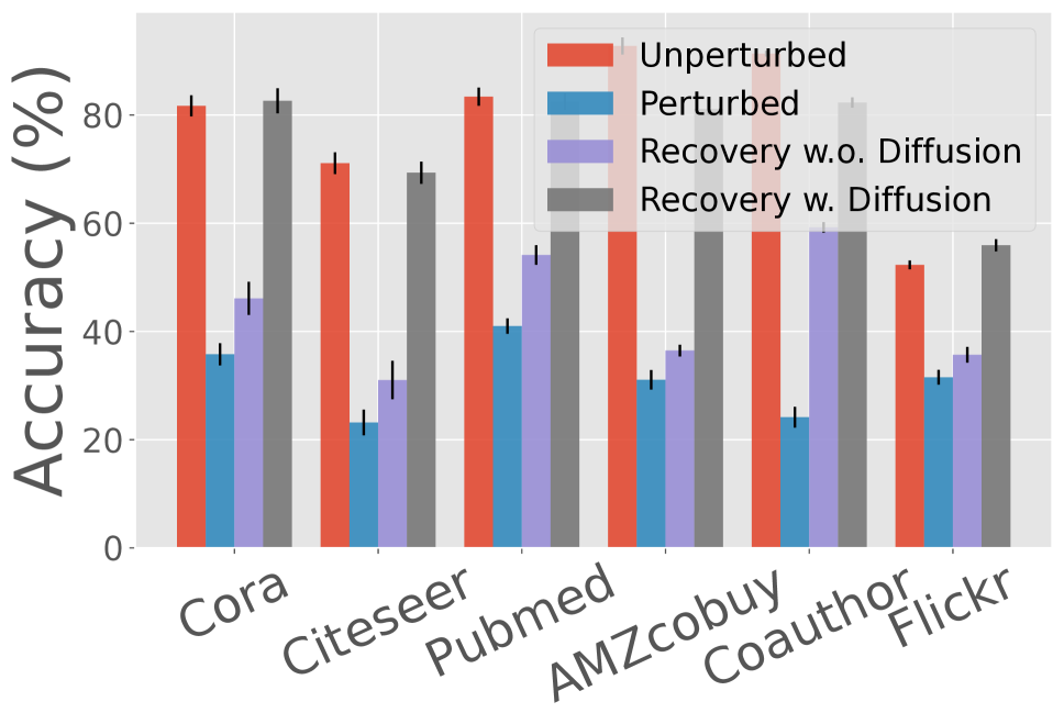
Figure 3: Ablation study of Gaussian diffusion. $p_{rdm}$ denotes the percentage of random-perturbator nodes over victim nodes. “Unperturbed” and “Perturbed” denote the accuracy on corresponding graphs, whereas “Recovery” denotes the recovered accuracy on perturbed graphs. Results affirm that applying Gaussian diffusion can generalize robust recovery to all perturbed graphs.

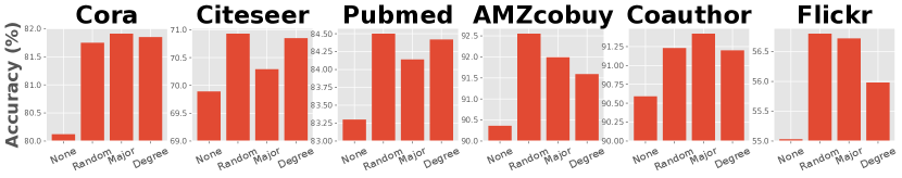
Figure 4: Investigation on the node embedding propagation with three types of samplers (random, major, and degree). “None” denotes the performance without using node embedding propagation.

Based on the vanilla architecture, we further examine whether Gaussian diffusion can generalize robust recovery on six perturbed graphs (random perturbations) under two different percentages of random-perturbator nodes over victim nodes (1% and 5%). As shown in each sub-figure of Fig. 3, the first two bars display the accuracy on unperturbed and perturbed graphs, whereas the last two bars present the recovered accuracy without/with applying Gaussian diffusion. This ablation study validates the effectiveness of Gaussian diffusion. Even in a gentle case, e.g., $p_{rdm}$=1%, our vanilla model cannot generalize robust recovery on Cora and Citeseer without applying Gaussian diffusion. In brief, the results indicate that applying Gaussian diffusion to the vanilla architecture can enhance the generalization capability of robust recoveries. Moreover, we dive deeper into the node embedding propagation with three types of samplers (Zhuang and Al Hasan 2022c) based on our previous architecture, applying Gaussian diffusion to the vanilla architecture. According to Fig. 4, propagating node embedding during training can further strengthen robustness. All three samplers are effective in node embedding propagation.

Methods	Cora		Citeseer		Pubmed		AMZcobuy		Coauthor		Flickr
	Acc.	Ent.	Acc.	Ent.	Acc.	Ent.	Acc.	Ent.	Acc.	Ent.	Acc.	Ent.
clean	81.43 (0.78)	26.47 (2.35)	71.06 (0.54)	61.53 (3.64)	84.34 (0.63)	37.49 (2.56)	92.75 (0.97)	14.22 (2.07)	91.50 (0.89)	8.82 (1.11)	52.06 (0.85)	66.29 (3.50)
rdmPert	48.42 (2.99)	5.98 (1.14)	24.46 (2.66)	6.06 (1.34)	42.80 (1.94)	1.81 (0.75)	55.29 (2.86)	21.85 (1.17)	44.24 (1.85)	17.21 (2.99)	42.86 (1.22)	69.66 (3.91)
retrain	82.63 (2.35)	29.04 (2.27)	69.96 (2.50)	55.11 (3.01)	82.11 (1.41)	35.44 (2.85)	92.17 (1.19)	10.82 (1.11)	89.80 (1.25)	10.28 (1.86)	56.80 (1.09)	7.96 (1.20)
infoSparse	72.26 (2.27)	36.49 (2.94)	64.10 (2.73)	68.11 (3.50)	76.58 (1.61)	47.37 (3.33)	90.34 (1.37)	17.19 (1.47)	86.91 (1.52)	16.33 (2.71)	46.33 (1.01)	76.53 (3.70)
retrain	73.42 (2.04)	29.77 (2.75)	64.46 (2.81)	32.74 (2.11)	77.56 (1.53)	35.99 (2.12)	91.39 (1.45)	9.36 (1.30)	87.58 (1.65)	7.42 (1.33)	49.71 (1.44)	6.99 (1.18)
advAttack	29.44 (2.60)	6.06 (1.59)	4.05 (1.53)	12.50 (1.19)	1.77 (0.81)	2.37 (0.94)	76.05 (1.02)	29.98 (2.16)	61.03 (1.98)	11.84 (1.82)	45.20 (2.13)	63.98 (2.80)
retrain	83.33 (2.54)	13.68 (2.49)	59.64 (2.28)	32.02 (2.67)	79.20 (1.60)	25.31 (3.35)	77.17 (1.81)	17.29 (1.64)	63.38 (1.52)	6.69 (0.97)	48.77 (2.09)	10.66 (2.31)

Table 1: Generalization test on our proposed model under three types of perturbations across six datasets. “clean” denotes the performance on the clean (unperturbed) graphs. “rdmPert”, “infoSparse”, and “advAttack” denote the performances on the corresponding perturbed graphs. “retrain” denotes the recovery in the corresponding scenario. We evaluate the performance five times “mean (std)” by classification accuracy (Acc.) and average normalized entropy (Ent.) on victim nodes.

Methods	Cora			Citeseer			Pubmed			AMZcobuy			Coauthor			Flickr
	Acc.	Ent.	Time	Acc.	Ent.	Time	Acc.	Ent.	Time	Acc.	Ent.	Time	Acc.	Ent.	Time	Acc.	Ent.	Time
GCN-Jaccard (Wu et al. 2019b)	69.47	88.91	2.41	57.94	89.83	2.28	67.13	77.29	5.63	89.15	91.32	8.87	86.99	96.23	9.38	49.37	95.19	53.15
GCN-SVD (Entezari et al. 2020)	47.89	88.95	2.66	34.33	88.34	2.96	73.28	80.89	8.16	82.85	91.94	10.12	75.78	95.51	16.56	50.13	96.45	71.22
DropEdge (Rong et al. 2019)	78.42	90.40	1.36	46.61	93.35	2.51	67.29	62.22	3.20	52.52	94.55	3.18	54.83	97.66	4.80	41.50	99.09	11.69
GRAND (Feng et al. 2020)	51.26	89.69	4.76	31.45	92.29	3.74	49.32	89.47	11.06	40.09	95.38	11.30	58.02	96.69	129.82	41.58	95.99	233.41
RGCN (Zhu et al. 2019)	66.32	98.02	10.78	60.94	98.15	10.96	83.20	87.05	32.95	76.53	96.82	32.35	89.25	97.88	184.21	50.11	96.33	290.10
ProGNN (Jin et al. 2020b)	47.37	87.17	202.01	34.89	77.19	340.68	49.25	85.93	3081.02	88.75	89.78	2427.02	82.16	95.85	3122.50	48.67	95.10	6201.90
MC Dropout (Gal 2016)	77.37	32.46	5.16	66.52	70.27	7.81	79.80	59.44	14.37	89.91	19.65	8.66	89.49	16.91	34.79	50.60	60.53	11.81
GraphSS (Zhuang et al. 2022a)	80.43	13.74	24.04	46.78	18.28	22.87	81.34	24.56	118.43	84.68	9.58	50.81	89.41	6.76	112.12	51.25	58.92	274.17
LInDT (Zhuang et al. 2022c)	83.68	20.40	33.32	70.53	57.26	66.61	83.64	32.55	145.76	91.89	8.58	76.05	90.58	7.44	155.46	52.01	57.55	319.42
Ours	84.01	29.57	21.30	71.49	53.75	21.60	84.25	34.16	105.44	92.56	10.06	40.96	91.22	9.85	95.01	57.15	8.91	211.01

Table 2: Comparison between competing methods and our model under the random perturbations scenario. Acc. (%) denotes classification accuracy. Ent. (%) denotes average normalized entropy. Time (s) denotes total runtime.

Generalization Test. We examine the generalization of our model (using the GCN aggregator with random sampler) under three types of perturbations, random perturbations (rdmPert), information sparsity (infoSparse), and adversarial attacks (advAttack), over six graphs, and present results in Tab. 1. We group the performance before/after retraining by the types of perturbations and highlight the highest Acc. and lowest Ent. on the results among these three groups. The results indicate that our model can help recover the accuracy in all datasets. However, the recovery may get a lower margin on extremely sparse graphs. This is possible because node aggregators and node embedding propagation may fail to capture the information when the graph structure and the features are extremely sparsified. Note that we sparsify the graph before applying adversarial attacks on AMZcobuy, Coauthor, and Flickr. For uncertainty, our model can reduce the normalized entropy (Ent.) in most cases compared to the Ent. on the clean graphs. In general, lower Ent. indicates lower uncertainty on the categorical distribution. However, this property is not always true when the graph is under severe perturbations. Worse prediction also leads to lower Ent., such as the results on Pubmed under advAttack (Acc.=1.77%, Ent.=2.37%). Overall, our goal is to achieve higher accuracy with relatively lower normalized entropy.

Comparison with Competing Methods. Tab. 2 compares performance between competing methods and our model under rdmPert ($p_{rdm}$=1%). The backbone model here is GCN. Both LInDT and our model use the random sampler. According to Tab. 2, our model outperforms all competing methods in Acc. and achieves low Ent. comparable to the state-of-the-art post-processing MCMC methods, LInDT. Compared among the post-processing methods (GraphSS, LInDT, and our model), MCMC methods (GraphSS and LInDT) can significantly decrease the Ent., whereas our model maintains a lower runtime than MCMC methods. Note that the main difference between MCMC methods and our model is that MCMC methods aim to approximate inferred labels to original labels as closely as possible on perturbed graphs, whereas our model is designed for generating node embedding for downstream tasks, which implies that our model has higher efficiency in the setting of streaming graphs (Further experiments are presented in Appendix).

Cora
Citeseer

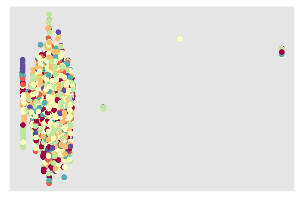
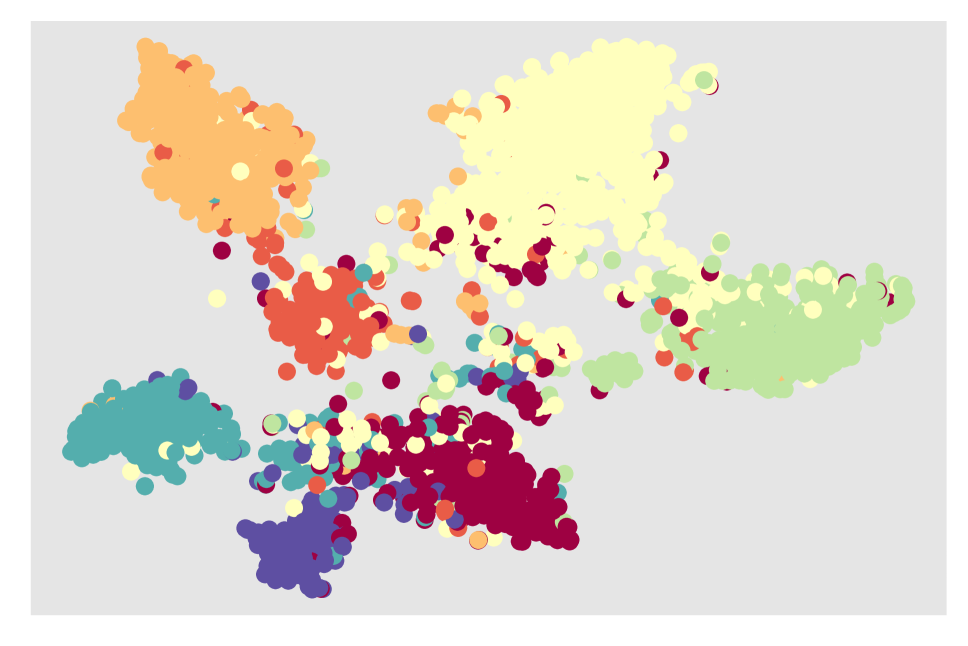
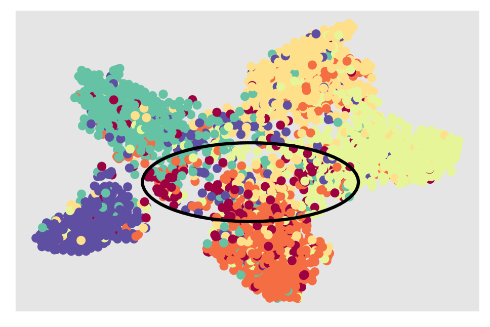
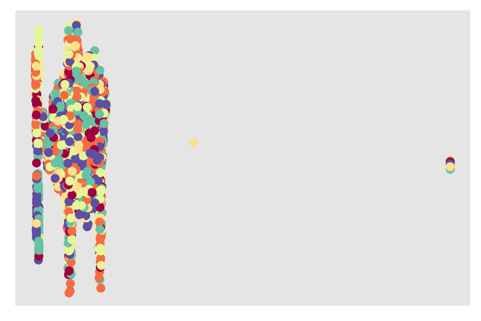
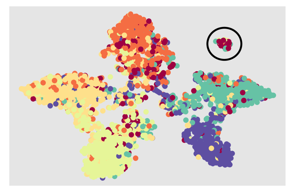
Figure 5: Visualization of node embedding on an unperturbed graph ($1^{st}$ column), a perturbed graph under 1% $p_{rdm}$ random perturbations ($2^{nd}$ column), and a perturbed graph after retraining ($3^{rd}$ column). Embeddings are colored by ground-truth labels.

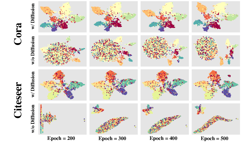
Figure 6: Visualization of the node embedding during the retraining process on two randomly perturbed graphs. “w/ Diffusion” and “w/o Diffusion” denote whether we apply Gaussian diffusion. “Epoch” denotes the retraining epoch.

Visualization. We visualize the node embedding via t-SNE on Cora and Citeseer as examples in Fig. 5. The visualization indicates that the retraining mechanism can help recover better node hidden representations in latent spaces on perturbed graphs. For example, in Citeseer (six classes), the nodes in the red class are mixed in the center ($1^{st}$ column) after initial training. Our proposed retraining mechanism can still partially classify these nodes in the upper-right corner ($3^{rd}$ column) under random perturbations. To better understand the retraining process, we visualize node embeddings during retraining on two randomly perturbed graphs ($p_{rdm}$=1%), Cora and Citeseer. The $1^{st}$ and $3^{rd}$ rows present results of applying Gaussian diffusion, whereas the $2^{nd}$ and $4^{th}$ rows present results without applying Gaussian diffusion. The retraining starts at the best checkpoint in the initial training process and stops by 500 epochs in total. We display a snapshot in the $200^{th}$, $300^{th}$, $400^{th}$, and $500^{th}$ epochs. The visualization validates the effectiveness of Gaussian diffusion.

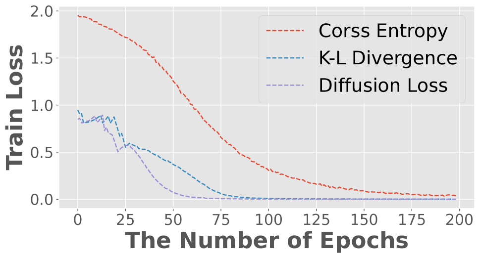
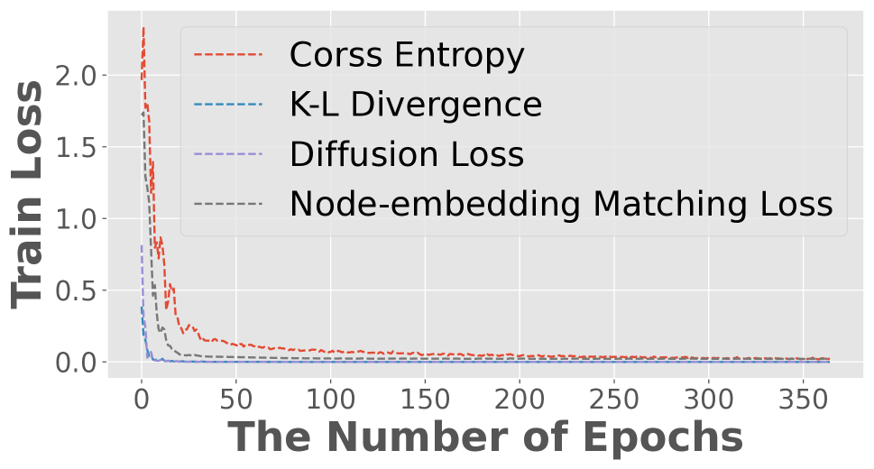
Figure 7: Convergence verification for each loss function during training (left) and retraining (right).

Convergence. We present loss curves during training (left) and retraining (right) for verifying the convergence of each loss on Cora as an example in Fig. 7. For better presentation, we rescale the loss of K-L divergence and diffusion to the same magnitude of cross entropy. The results verify that all losses can eventually converge. Note that the retraining starts from the best checkpoint in the training stage and ends in 500 epochs (including the first 200 training epochs).

Parameters. We tune the diffusion rate $\gamma$ within a given range on the validation set. The maximum value of the range $\gamma_{max}$ is 0.9999. The minimum value of the range $\gamma_{min}$ changes from 0.5 to 0.99. As displayed in Fig. 8, we select the $\gamma_{min}$ as 0.6, 0.98, 0.99, 0.84, 0.96, and 0.96 on six datasets. Besides, we follow the same setting as that in Tab. 2 and analyze the coefficient sensitivity for each loss by control variables on Cora as an example in Fig. 9. Cross-entropy is crucial to classification as accuracy drops dramatically after muting $\mathcal{L}_{ce}$. Increasing the percentage of $\mathcal{L}_{nm}$ can boost recovery. Choosing appropriate $\mathcal{L}_{kl}$ and $\mathcal{L}_{df}$ can help achieve higher accuracy. We assign equal weight to each loss and verify that our model can generalize to these public datasets without further tuning the coefficient.

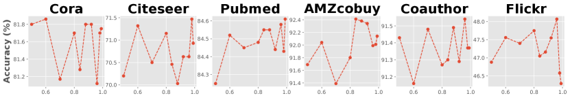
Figure 8: Analysis of diffusion rate (x-axis: minimum values of a range for diffusion rate; y-axis: validation accuracy).

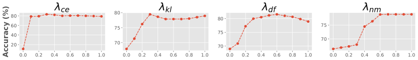
Figure 9: Investigation of coefficient sensitivity for each loss on Cora (x-axis: the value of $\lambda$; y-axis: validation accuracy).

Limitation. Though we release dependency on a well-predicted prior compared to MCMC methods, our model still gets a lower margin on extremely sparse graphs due to a lack of information for node aggregation and propagation. In the future, we could utilize the inverse diffusion process to complete graph structures. Besides, node embedding propagation may not perform strongly on heterogeneous graphs due to the assumption of graph homophily property.

Related Work

Besides discussing background in Introduction, we further introduce related works as follows: Variational diffusion models have achieved great impact as a kind of generative model in recent two years (Song, Meng, and Ermon 2020; Li et al. 2020; Rey, Menkovski, and Portegies 2019). Following this impact, an increasing number of studies have started exploring how variational diffusion can contribute to graph structural data (Zhou et al. 2020; Ling et al. 2022). Learning robust node representation via variational diffusion is a promising direction in the early stage. Label propagation techniques have been widely used in the semi-supervised learning paradigm (Zhu and Ghahramani 2002; Wang and Zhang 2007; Ugander and Backstrom 2013; Gong et al. 2016; Iscen et al. 2019). Recent studies utilize this technique to learn robust GNNs (Huang et al. 2020; Wang and Leskovec 2020).

Conclusion

We aim to learn robust node representations for recovering node classifications on perturbed graphs. While infusing Gaussian noise in hidden layers is an appealing strategy for enhancing robustness, our experiments show that this strategy may result in over-smoothing issues during node aggregation. Thus, we propose the Graph Variational Diffusion Network (GVDN), a new node encoder that effectively manipulates Gaussian noise to improve robustness while alleviating over-smoothing issues by two mechanisms: Gaussian diffusion and node embedding propagation. We also design a retraining mechanism using generated node embeddings for recovery. Extensive experiments validate the effectiveness of our proposed model across six public graph datasets.

Broader Impact

We confirm that we fulfill the author’s responsibilities. As an indispensable component of AI algorithms, GNNs are extensively utilized to learn node representations in graph-structure data. Thus, it is significant to improve the robustness of GNNs against perturbations. From a social perspective, our model can be applied to enhance the robustness in downstream node classification tasks in real-world scenarios, such as user profiling in online social networks. From a technical perspective, our model can benefit other research fields, such as robust node classifications in noise-label or sparse-label environments (Appendix).

Appendix A APPENDIX

In the appendix, we first describe the details of datasets, implementation of perturbations, hyper-parameters for both our model and competing methods, evaluation metrics, and hardware/software. We further present supplementary experiments in the second section.

Appendix B Experimental Settings

Datasets

Tab. 3 presents statistics of six public node-labeled graph datasets. Cora, Citeseer, and Pubmed are famous citation graph data (Sen et al. 2008). AMZcobuy comes from the photo segment of the Amazon co-purchase graph (Shchur et al. 2018). Coauthor is co-authorship graphs of computer science based on the Microsoft Academic Graph from the KDD Cup 2016 challenge . Flickr is a image-relationship graph dataset (Zeng et al. 2019). The first five graphs are widely used in the study of robust node representation learning. We additionally select Flickr to validate that our proposed model can achieve robust performance on a graph with a larger size and lower EHR.

Dataset	$\left|\mathcal{V}\right|$	$\left|\mathcal{E}\right|$	$\left|F\right|$	$\left|C\right|$	Avg.D	EHR(%)
Cora	2,708	10,556	1,433	7	4.99	81.00
Citeseer	3,327	9,228	3,703	6	3.72	73.55
Pubmed	19,717	88,651	500	3	5.50	80.24
AMZcobuy	7,650	287,326	745	8	32.77	82.72
Coauthor	18,333	327,576	6,805	15	10.01	80.81
Flickr	89,250	899,756	500	7	11.07	31.95

Table 3: Statistics of datasets. $\left|\mathcal{V}\right|$, $\left|\mathcal{E}\right|$, $\left|F\right|$, and $\left|C\right|$ denote the number of nodes, edges, features, and classes, respectively. Avg.D denotes the average degree of test nodes. EHR denotes the edge homophily ratio.

Implementation of Perturbations

We examine the generalization of our model under three scenarios of perturbations, whose settings follow (Zhuang and Al Hasan 2022c).
1) Random perturbations (rdmPert) simulate a non-malicious perturbator in OSNs that randomly connects with many other normal users for commercial purposes. In the experiments, we denote the percentage of random-perturbator nodes over validation/test nodes (a.k.a. victim nodes) as $p_{rdm}$ and restrict the number of connections from each perturbator to $\frac{1}{p_{rdm}}$. Except for specific statements, we select $p_{rdm}=1\%$ in this paper. Note that rdmPert doesn’t apply gradient-based attacks, such as FGSM (Goodfellow, Shlens, and Szegedy 2014), PGD (Madry et al. 2017), etc.
2) Information sparsity (infoSparse) sparsifies 90% links and 100% features of the victim nodes ($L\&F$) on validation/test graphs.
3) Adversarial attacks (advAttack) execute node-level direct evasion non-targeted attacks (Zügner, Akbarnejad, and Günnemann 2018) on both links and features ($L\&F$) of the victim nodes on sparse graphs as such kind of attacks may fail on denser graphs. To ensure the sparsity, we sparse the denser graphs (AMZcobuy and Coauthor) and select the victim nodes whose total degrees are within (0, 10) for attacks. The intensity of perturbation $n_{pert}$ is set as 2 for all datasets. The ratio of $n_{pert}$ between applying on links and applying on features is 1: 10.

Hyper-parameters and Settings of Our Model

Our experiments involve four two-layer classic GNNs (GCN (Kipf and Welling 2016a), GraphSAGE (Hamilton, Ying, and Leskovec 2017), SGC (Wu et al. 2019a), and GAT (Veličković et al. 2018)) with 200 hidden units and a ReLU activation function. Their hyper-parameters are summarized in Tab. 4. Within these GNNs, we select GCN as the backbone node aggregator for our model. Both these four GNNs and our model are trained by the Adam optimizer with a $1\times 10^{-3}$ learning rate and converged within 200 epochs of training on all datasets. The weights of these node aggregators are initialized by Glorot initialization. Only the weight $\mathbf{W}_{z}$ in our model is initialized by He initialization. The size of weights is summarized in Tab. 5. We set all $\lambda$ values as 1.0 in the experiments. We select the $\gamma_{min}$ based on the best validation accuracy. For retraining, our model is retrained to 500 epochs in total. In the ablation study, generalization test, and comparison of competing methods (including the inference runtime), we run experiments five times and report the mean values (some cases are reported as “mean (std)”). For convergence verification, analysis of parameters, and further explorations, we only run the experiment once.

Model	#Hops	Aggregator	#Heads	Activation	Dropout
$\mathbf{GCN}$	$\times$	$\times$	$\times$	ReLU	0.5
$\mathbf{SGC}$	2	$\times$	$\times$	$\times$	0.5
$\mathbf{GraphSAGE}$	$\times$	gcn	$\times$	ReLU	0.5
$\mathbf{GAT}$	$\times$	$\times$	3	ReLU	0.5

Table 4: Model architecture of four classic GNNs.

$\mathbf{Weights}$	$\mathbf{W}_{h}^{(0)}$	$\mathbf{W}_{\mu}$	$\mathbf{W}_{\sigma}$	$\mathbf{W}_{z}$	$\mathbf{W}_{h}^{(1)}$
$\mathbf{Size}$	$d\times h$	$d\times h$	$d\times h$	$|\mathbf{Z}|\times h$	$h\times K$

Table 5: Size of weights in our model. d, h, $|\mathbf{Z}|$, and K denote the number of features, hidden units, nodes in $\mathbf{Z}$, and classes, respectively.

Hyper-parameters	Cora	Citeseer	Pubmed	AMZcobuy	Coauthor	Flickr
Hidden units	200	200	200	200	200	200
Dropout rate	0.8	0.8	0.5	0.5	0.5	0.3
Learning rate	1e-2	9e-3	1e-2	1e-2	1e-2	1e-2
Weight decay	5e-3	1e-3	1e-3	1e-2	1e-3	1e-3
Use BN	$\times$	$\times$	$\times$	$\checkmark$	$\times$	$\times$

Table 6: Hyper-parameters of DropEdge in this paper.

Hyper-parameters	Cora	Citeseer	Pubmed	AMZcobuy	Coauthor	Flickr
Propagation step	8	2	5	5	5	5
Data augmentation times	4	2	4	3	3	4
CR loss coefficient	1.0	0.7	1.0	0.9	0.9	1.0
Sharpening temperature	0.5	0.3	0.2	0.4	0.4	0.3
Learning rate	0.01	0.01	0.2	0.2	0.2	0.2
Early stopping patience	200	200	100	100	100	200
Input dropout	0.5	0.0	0.6	0.6	0.6	0.6
Hidden dropout	0.5	0.2	0.8	0.5	0.5	0.5
Use BN	$\times$	$\times$	$\checkmark$	$\checkmark$	$\checkmark$	$\checkmark$

Table 7: Hyper-parameters of GRAND in this paper.

Hyper-parameters of Competing Methods

We compare our model with nine competing methods. GCN-Jaccard, GCN-SVD, and DropEdge belong to pre-processing methods. GRAND, RGCN, and ProGNN are categorized as inter-processing methods. GraphSS and LInDT are classified as post-processing methods. Both MC Dropout and post-processing methods are used for measuring the uncertainty purposes. We present hyper-parameters of competing methods for reproducibility purposes. All models are trained by Adam optimizer. Note that GCN-Jaccard, GCN-SVD, DropEdge, ProGNN, MC Dropout, GraphSS, and LInDT also select GCN as the backbone model.

• GCN-Jaccard (Wu et al. 2019b) preprocesses the graph by eliminating suspicious connections, whose Jaccard similarity of node’s features is smaller than a given threshold. The similarity threshold is 0.01. Hidden units are 200. The dropout rate is 0.5. Training epochs are 300.

• GCN-SVD (Entezari et al. 2020) proposes another preprocessing approach with low-rank approximation on the perturbed graph to mitigate the negative effects from high-rank attacks, such as Nettack (Zügner, Akbarnejad, and Günnemann 2018). The number of singular values is 15. Hidden units are 200. The dropout rate is 0.5. Training epochs are 300.

• DropEdge (Rong et al. 2019) randomly removes several edges from the input graph in each training epoch. We choose 1 base block layer and train this model with 300 epochs. Other parameters are mentioned in Tab. 6.

• GRAND (Feng et al. 2020) proposes random propagation and consistency regularization strategies to address the issues of over-smoothing and non-robustness of GCNs. The model is trained with 200 epochs. The hidden units, drop node rate, and L2 weight decay are 200, 0.5, and $5\times 10^{-4}$. Other parameters are reported in Tab. 7.

• RGCN (Zhu et al. 2019) adopts Gaussian distributions as hidden representations of nodes to mitigate the negative effects of adversarial attacks. We set up $\gamma$ as 1, $\beta_{1}$ and $\beta_{2}$ as $5\times 10^{-4}$ on all datasets. The hidden units for each dataset are 64, 64, 128, 1024, 1024, and 2014, respectively. The dropout rate is 0.6. The learning rate is 0.01. The training epochs are 400.

• ProGNN (Jin et al. 2020b) jointly learns the structural graph properties and iteratively reconstructs the clean graph to reduce the effects of adversarial structure. We select $\alpha$, $\beta$, $\gamma$, and $\lambda$ as $5\times 10^{-4}$, 1.5, 1.0, and 0.0, respectively. The hidden units are 200. The dropout rate is 0.5. The learning rate is 0.01. Weight decay is $5\times 10^{-4}$. The training epochs are 100.

• MC Dropout (Gal and Ghahramani 2016) develops a dropout framework that approximates Bayesian inference in deep Gaussian processes. We follow the same settings as our proposed model except for selecting the optimal dropout rate for each dataset as 0.7, 0.3, 0.9, 0.6, 0.8, and 0.3, respectively. Note that MC Dropout will apply dropout in test data.

• GraphSS (Zhuang and Al Hasan 2022a) approximates inferred labels to original labels on perturbed graphs as closely as possible by iterative Bayesian label transition. We follow the same settings as GraphSS. The number of epochs for inference, retraining, and warm-up steps is 100, 60, and 40, respectively. The $\alpha$ is fixed as 1.0.

• LInDT (Zhuang and Al Hasan 2022c) proposes a new topology-based label sampling method with dynamic Dirichlet prior to boost the performance of Bayesian label transition against topological perturbations. We follow the same settings as LInDT. The number of inference epochs is 100, 200, 80, 100, 90, and 100 for each dataset. The number of retraining epochs and warm-up steps remains at 60 and 40, respectively. The $\alpha$ value is 0.1, 0.3, 1.0, 0.7, 0.1, and 0.1 for each dataset in the beginning and will be dynamically updated during the inference.

Evaluation Metrics

In this work, we evaluate the performance by classification accuracy (Acc.) and average normalized entropy (Ent.), which is formulated in Eq. 14. Acc. is a classic metric to evaluate the performance of node classifications. Higher Acc. indicates better node classification. We use Ent. to evaluate the uncertainty. Lower Ent. portrays lower uncertainty on the nodes’ categorical distributions.

$$\mathbf{Ent}(\mathbf{X})=-\frac{1}{N}\sum_{i=1}^{N}\sum_{j=1}^{d}\frac{p(x_{i,j})\ln{(p(x_{i,j}))}}{\ln{(d)}}.$$ (14)

Hardware and Software

All experiments are conducted on the server with the following configurations:

• Operating System: Ubuntu 18.04.5 LTS

• CPU: Intel(R) Xeon(R) Gold 6258R CPU @ 2.70 GHz

• GPU: NVIDIA Tesla V100 PCIe 16GB

• Software: Python 3.8, PyTorch 1.7.

Appendix C Supplementary Experiments

Comparison of Inference Runtime

Tab. 8 presents the average inference runtime among MCMC methods and our model in ten streaming sub-graphs. Our model has a significantly lower runtime over all datasets as our retraining mechanism only retrains the model once for the same type of perturbations, whereas MCMC methods must run the inference model on top of GNNs to output the inferred labels for each sub-graph. This advantage implies that our model can be applied to various online downstream tasks for robust inference.

	Cora	Citeseer	Pubmed	AMZcobuy	Coauthor	Flickr
GraphSS	23.66	24.71	113.59	51.33	109.82	276.50
LInDT	32.04	66.50	143.88	76.10	156.08	318.33
Ours	2.02	3.29	10.78	4.19	9.31	21.35

Table 8: The average inference runtime (in seconds) among MCMC methods and our model in streaming settings.

Discussion on Other Competing Methods

Besides comparing the inference runtime, we have several observations in other competing methods, as follows: First, both post-processing methods and MC Dropout can help decrease the Ent. on all datasets. Second, RGCN obtains higher accuracy on larger graphs. We argue that adopting Gaussian distributions in hidden layers can reduce the negative impacts on larger perturbed graphs. Third, ProGNN performs better on denser graphs. This is possible because ProGNN utilizes the properties of the graph structure to mitigate perturbations while denser graphs preserve the plentiful topological relationships. From the perspective of runtime (in seconds), we observe that GCN-Jaccard, GCN-SVD, DropEdge, and MC dropout consume much less time than other methods. These are reasonable because these methods mainly process the graph structure by dropping edges or hidden units. However, these methods may not be effective on real-world social graphs as the graph structure of OSNs is dynamically changing. On the contrary, ProGNN consumes much more time as the size of graphs increases because it preserves low rank and sparsity properties via iterative reconstructions.

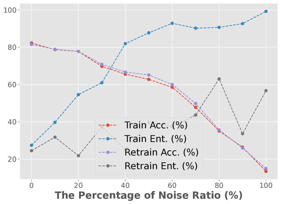
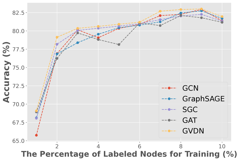
Figure 10: Further explorations under the setting of noise labeling (left side) and sparse labeling (right side).

Further Explorations

Besides recovering the performance on the perturbed graphs, we explore whether our model can benefit other research fields on Cora. We first investigate the performance of our model under the noisy labels setting (left side of Fig. 10). In this experiment, we inject the noises into the train labels by randomly replacing the ground-truth labels with another label, chosen uniformly. We denote the percentage of the noises as noise ratio, $nr$, and adjust this ratio from 0% to 100%. As expected, the accuracy decreases as the $nr$ increases. However, our proposed retraining mechanism can maintain the normalized entropy at a relatively low level compared to the result before retraining. This result indicates that our model could contribute to the uncertainty estimation on the graphs with noisy labeling. Furthermore, we examine whether our model can work under the sparse labeling setting (right side of Fig. 10). In this setting, the percentage of the labeled train nodes changes from 1% to 10%. The results reveal that our model can maintain robust performance when the labeling rate is not less than 2% and slightly outperforms the other four popular GNNs without retraining.

References

- Bo et al. (2021) Bo, D.; Wang, X.; Shi, C.; and Shen, H. 2021. Beyond low-frequency information in graph convolutional networks. In Proceedings of the AAAI Conference on Artificial Intelligence, volume 35, 3950–3957.
- Breuer, Eilat, and Weinsberg (2020) Breuer, A.; Eilat, R.; and Weinsberg, U. 2020. Friend or Faux: Graph-Based Early Detection of Fake Accounts on Social Networks. In Proceedings of The Web Conference 2020, 1287–1297.
- Bruna et al. (2013) Bruna, J.; Zaremba, W.; Szlam, A.; and LeCun, Y. 2013. Spectral networks and locally connected networks on graphs. arXiv preprint arXiv:1312.6203.
- Chang et al. (2021) Chang, H.; Rong, Y.; Xu, T.; Bian, Y.; Zhou, S.; Wang, X.; Huang, J.; and Zhu, W. 2021. Not All Low-Pass Filters are Robust in Graph Convolutional Networks. Advances in Neural Information Processing Systems, 34.
- Chen et al. (2019) Chen, W.; Gu, Y.; Ren, Z.; He, X.; Xie, H.; Guo, T.; Yin, D.; and Zhang, Y. 2019. Semi-supervised User Profiling with Heterogeneous Graph Attention Networks. In IJCAI, volume 19, 2116–2122.
- Dai et al. (2018) Dai, H.; Li, H.; Tian, T.; Huang, X.; Wang, L.; Zhu, J.; and Song, L. 2018. Adversarial attack on graph structured data. In International conference on machine learning, 1115–1124. PMLR.
- Defferrard, Bresson, and Vandergheynst (2016) Defferrard, M.; Bresson, X.; and Vandergheynst, P. 2016. Convolutional neural networks on graphs with fast localized spectral filtering. In Advances in neural information processing systems, 3844–3852.
- Entezari et al. (2020) Entezari, N.; Al-Sayouri, S. A.; Darvishzadeh, A.; and Papalexakis, E. E. 2020. All you need is low (rank) defending against adversarial attacks on graphs. In Proceedings of the 13th International Conference on Web Search and Data Mining, 169–177.
- Fang et al. (2016) Fang, H.; Wu, F.; Zhao, Z.; Duan, X.; Zhuang, Y.; and Ester, M. 2016. Community-based question answering via heterogeneous social network learning. In Proceedings of the AAAI conference on artificial intelligence, volume 30.
- Feng et al. (2020) Feng, W.; Zhang, J.; Dong, Y.; Han, Y.; Luan, H.; Xu, Q.; Yang, Q.; Kharlamov, E.; and Tang, J. 2020. Graph Random Neural Networks for Semi-Supervised Learning on Graphs. Advances in Neural Information Processing Systems, 33.
- Gal and Ghahramani (2016) Gal, Y.; and Ghahramani, Z. 2016. Dropout as a bayesian approximation: Representing model uncertainty in deep learning. In international conference on machine learning, 1050–1059. PMLR.
- Godwin et al. (2021) Godwin, J.; Schaarschmidt, M.; Gaunt, A. L.; Sanchez-Gonzalez, A.; Rubanova, Y.; Veličković, P.; Kirkpatrick, J.; and Battaglia, P. 2021. Simple gnn regularisation for 3d molecular property prediction and beyond. In International conference on learning representations.
- Gong et al. (2016) Gong, C.; Tao, D.; Liu, W.; Liu, L.; and Yang, J. 2016. Label propagation via teaching-to-learn and learning-to-teach. IEEE transactions on neural networks and learning systems, 28(6): 1452–1465.
- Goodfellow, Shlens, and Szegedy (2014) Goodfellow, I. J.; Shlens, J.; and Szegedy, C. 2014. Explaining and harnessing adversarial examples. arXiv preprint arXiv:1412.6572.
- Hamilton, Ying, and Leskovec (2017) Hamilton, W.; Ying, Z.; and Leskovec, J. 2017. Inductive representation learning on large graphs. In Advances in neural information processing systems, 1024–1034.
- Ho, Jain, and Abbeel (2020) Ho, J.; Jain, A.; and Abbeel, P. 2020. Denoising diffusion probabilistic models. Advances in Neural Information Processing Systems, 33: 6840–6851.
- Huang et al. (2020) Huang, Q.; He, H.; Singh, A.; Lim, S.-N.; and Benson, A. R. 2020. Combining label propagation and simple models out-performs graph neural networks. arXiv preprint arXiv:2010.13993.
- Iscen et al. (2019) Iscen, A.; Tolias, G.; Avrithis, Y.; and Chum, O. 2019. Label propagation for deep semi-supervised learning. In Proceedings of the IEEE/CVF Conference on Computer Vision and Pattern Recognition, 5070–5079.
- Jin et al. (2021) Jin, W.; Derr, T.; Wang, Y.; Ma, Y.; Liu, Z.; and Tang, J. 2021. Node similarity preserving graph convolutional networks. In Proceedings of the 14th ACM International Conference on Web Search and Data Mining.
- Jin et al. (2020a) Jin, W.; Li, Y.; Xu, H.; Wang, Y.; Ji, S.; Aggarwal, C.; and Tang, J. 2020a. Adversarial Attacks and Defenses on Graphs: A Review, A Tool and Empirical Studies. arXiv preprint arXiv:2003.00653.
- Jin et al. (2020b) Jin, W.; Ma, Y.; Liu, X.; Tang, X.; Wang, S.; and Tang, J. 2020b. Graph structure learning for robust graph neural networks. In Proceedings of the 26th ACM SIGKDD International Conference on Knowledge Discovery & Data Mining, 66–74.
- Kingma et al. (2021) Kingma, D.; Salimans, T.; Poole, B.; and Ho, J. 2021. Variational diffusion models. Advances in neural information processing systems, 34: 21696–21707.
- Kingma and Welling (2013) Kingma, D. P.; and Welling, M. 2013. Auto-encoding variational bayes. arXiv preprint arXiv:1312.6114.
- Kipf and Welling (2016a) Kipf, T. N.; and Welling, M. 2016a. Semi-supervised classification with graph convolutional networks. arXiv preprint arXiv:1609.02907.
- Kipf and Welling (2016b) Kipf, T. N.; and Welling, M. 2016b. Variational graph auto-encoders. arXiv preprint arXiv:1611.07308.
- Li et al. (2020) Li, H.; Lindenbaum, O.; Cheng, X.; and Cloninger, A. 2020. Variational diffusion autoencoders with random walk sampling. In European Conference on Computer Vision, 362–378. Springer.
- Ling et al. (2022) Ling, C.; Jiang, J.; Wang, J.; and Liang, Z. 2022. Source Localization of Graph Diffusion via Variational Autoencoders for Graph Inverse Problems. In Proceedings of the 28th ACM SIGKDD Conference on Knowledge Discovery and Data Mining, 1010–1020.
- Liu et al. (2021) Liu, X.; Jin, W.; Ma, Y.; Li, Y.; Liu, H.; Wang, Y.; Yan, M.; and Tang, J. 2021. Elastic graph neural networks. In International Conference on Machine Learning. PMLR.
- Madry et al. (2017) Madry, A.; Makelov, A.; Schmidt, L.; Tsipras, D.; and Vladu, A. 2017. Towards deep learning models resistant to adversarial attacks. arXiv preprint arXiv:1706.06083.
- Nt and Maehara (2019) Nt, H.; and Maehara, T. 2019. Revisiting graph neural networks: All we have is low-pass filters. arXiv preprint arXiv:1905.09550.
- Pan et al. (2018) Pan, S.; Hu, R.; Long, G.; Jiang, J.; Yao, L.; and Zhang, C. 2018. Adversarially regularized graph autoencoder for graph embedding. arXiv preprint arXiv:1802.04407.
- Rey, Menkovski, and Portegies (2019) Rey, L. A. P.; Menkovski, V.; and Portegies, J. W. 2019. Diffusion variational autoencoders. arXiv preprint arXiv:1901.08991.
- Rong et al. (2019) Rong, Y.; Huang, W.; Xu, T.; and Huang, J. 2019. Dropedge: Towards deep graph convolutional networks on node classification. arXiv preprint arXiv:1907.10903.
- Sen et al. (2008) Sen, P.; Namata, G.; Bilgic, M.; Getoor, L.; Galligher, B.; and Eliassi-Rad, T. 2008. Collective classification in network data. AI magazine.
- Shchur et al. (2018) Shchur, O.; Mumme, M.; Bojchevski, A.; and Günnemann, S. 2018. Pitfalls of Graph Neural Network Evaluation. Relational Representation Learning Workshop, NeurIPS 2018.
- Song, Meng, and Ermon (2020) Song, J.; Meng, C.; and Ermon, S. 2020. Denoising diffusion implicit models. arXiv preprint arXiv:2010.02502.
- Sun et al. (2018a) Sun, L.; Dou, Y.; Yang, C.; Wang, J.; Yu, P. S.; and Li, B. 2018a. Adversarial attack and defense on graph data: A survey. arXiv preprint arXiv:1812.10528.
- Sun et al. (2018b) Sun, Z.; Yang, J.; Zhang, J.; Bozzon, A.; Huang, L.-K.; and Xu, C. 2018b. Recurrent knowledge graph embedding for effective recommendation. In Proceedings of the 12th ACM conference on recommender systems, 297–305.
- Tam and Dunson (2020) Tam, E.; and Dunson, D. 2020. Fiedler regularization: Learning neural networks with graph sparsity. In International Conference on Machine Learning, 9346–9355. PMLR.
- Ugander and Backstrom (2013) Ugander, J.; and Backstrom, L. 2013. Balanced label propagation for partitioning massive graphs. In Proceedings of the sixth ACM international conference on Web search and data mining, 507–516.
- Van Ravenzwaaij, Cassey, and Brown (2018) Van Ravenzwaaij, D.; Cassey, P.; and Brown, S. D. 2018. A simple introduction to Markov Chain Monte–Carlo sampling. Psychonomic bulletin & review, 25(1): 143–154.
- Veličković et al. (2018) Veličković, P.; Cucurull, G.; Casanova, A.; Romero, A.; Liò, P.; and Bengio, Y. 2018. Graph Attention Networks. In International Conference on Learning Representations.
- Wang and Zhang (2007) Wang, F.; and Zhang, C. 2007. Label propagation through linear neighborhoods. IEEE Transactions on Knowledge and Data Engineering, 20(1): 55–67.
- Wang and Leskovec (2020) Wang, H.; and Leskovec, J. 2020. Unifying graph convolutional neural networks and label propagation. arXiv preprint arXiv:2002.06755.
- Wu et al. (2019a) Wu, F.; Zhang, T.; Souza Jr, A. H. d.; Fifty, C.; Yu, T.; and Weinberger, K. Q. 2019a. Simplifying graph convolutional networks. arXiv preprint arXiv:1902.07153.
- Wu et al. (2019b) Wu, H.; Wang, C.; Tyshetskiy, Y.; Docherty, A.; Lu, K.; and Zhu, L. 2019b. Adversarial examples on graph data: Deep insights into attack and defense. arXiv preprint arXiv:1903.01610.
- Xiong, Power, and Callan (2017) Xiong, C.; Power, R.; and Callan, J. 2017. Explicit semantic ranking for academic search via knowledge graph embedding. In Proceedings of the 26th international conference on world wide web, 1271–1279.
- Ye and Ji (2021) Ye, Y.; and Ji, S. 2021. Sparse graph attention networks. IEEE Transactions on Knowledge and Data Engineering.
- Ying et al. (2018) Ying, R.; He, R.; Chen, K.; Eksombatchai, P.; Hamilton, W. L.; and Leskovec, J. 2018. Graph convolutional neural networks for web-scale recommender systems. In Proceedings of the 24th ACM SIGKDD international conference on knowledge discovery & data mining, 974–983.
- Zeng et al. (2019) Zeng, H.; Zhou, H.; Srivastava, A.; Kannan, R.; and Prasanna, V. 2019. Graphsaint: Graph sampling based inductive learning method. arXiv preprint arXiv:1907.04931.
- Zhou et al. (2020) Zhou, F.; Yang, Q.; Zhong, T.; Chen, D.; and Zhang, N. 2020. Variational graph neural networks for road traffic prediction in intelligent transportation systems. IEEE Transactions on Industrial Informatics, 17(4): 2802–2812.
- Zhu et al. (2019) Zhu, D.; Zhang, Z.; Cui, P.; and Zhu, W. 2019. Robust graph convolutional networks against adversarial attacks. In Proceedings of the 25th ACM SIGKDD International Conference on Knowledge Discovery & Data Mining.
- Zhu et al. (2020) Zhu, J.; Yan, Y.; Zhao, L.; Heimann, M.; Akoglu, L.; and Koutra, D. 2020. Beyond homophily in graph neural networks: Current limitations and effective designs. Advances in Neural Information Processing Systems, 33: 7793–7804.
- Zhu and Ghahramani (2002) Zhu, X.; and Ghahramani, Z. 2002. Learning from labeled and unlabeled data with label propagation.
- Zhuang and Al Hasan (2022a) Zhuang, J.; and Al Hasan, M. 2022a. Defending Graph Convolutional Networks against Dynamic Graph Perturbations via Bayesian Self-Supervision. Proceedings of the AAAI Conference on Artificial Intelligence, 36(4): 4405–4413.
- Zhuang and Al Hasan (2022b) Zhuang, J.; and Al Hasan, M. 2022b. Deperturbation of Online Social Networks via Bayesian Label Transition. In Proceedings of the 2022 SIAM International Conference on Data Mining (SDM), 603–611. SIAM.
- Zhuang and Al Hasan (2022c) Zhuang, J.; and Al Hasan, M. 2022c. Robust Node Classification on Graphs: Jointly from Bayesian Label Transition and Topology-based Label Propagation. In Proceedings of the 31st ACM International Conference on Information & Knowledge Management, 2795–2805.
- Zhuang and Hasan (2022) Zhuang, J.; and Hasan, M. A. 2022. How Does Bayesian Noisy Self-Supervision Defend Graph Convolutional Networks? Neural Processing Letters, 1–22.
- Zügner, Akbarnejad, and Günnemann (2018) Zügner, D.; Akbarnejad, A.; and Günnemann, S. 2018. Adversarial attacks on neural networks for graph data. In Proceedings of the 24th ACM SIGKDD International Conference on Knowledge Discovery & Data Mining, 2847–2856.