Deep Learning-based MRI Reconstruction with Artificial Fourier Transform (AFT)-Net

Abstract

The deep complex-valued neural network provides a powerful way to leverage complex number operations and representations, which has succeeded in several phase-based applications. However, most previously published networks have not fully accessed the impact of complex-valued networks in the frequency domain. Here, we introduced a unified complex-valued deep learning framework - artificial Fourier transform network (AFT-Net) - which combined domain-manifold learning and complex-valued neural networks. The AFT-Net can be readily used to solve the image inverse problems in domain-transform, especially for accelerated magnetic resonance imaging (MRI) reconstruction and other applications. While conventional methods only accept magnitude images, the proposed method takes raw k-space data in the frequency domain as inputs, allowing a mapping between the k-space domain and the image domain to be determined through cross-domain learning. We show that AFT-Net achieves superior accelerated MRI reconstruction and is comparable to existing approaches. Also, our approach can be applied to different tasks like denoised MRS reconstruction and different datasets with various contrasts. The AFT-Net presented here is a valuable preprocessing component for different preclinical studies and provides an innovative alternative for solving inverse problems in imaging and spectroscopy.

1 Introduction

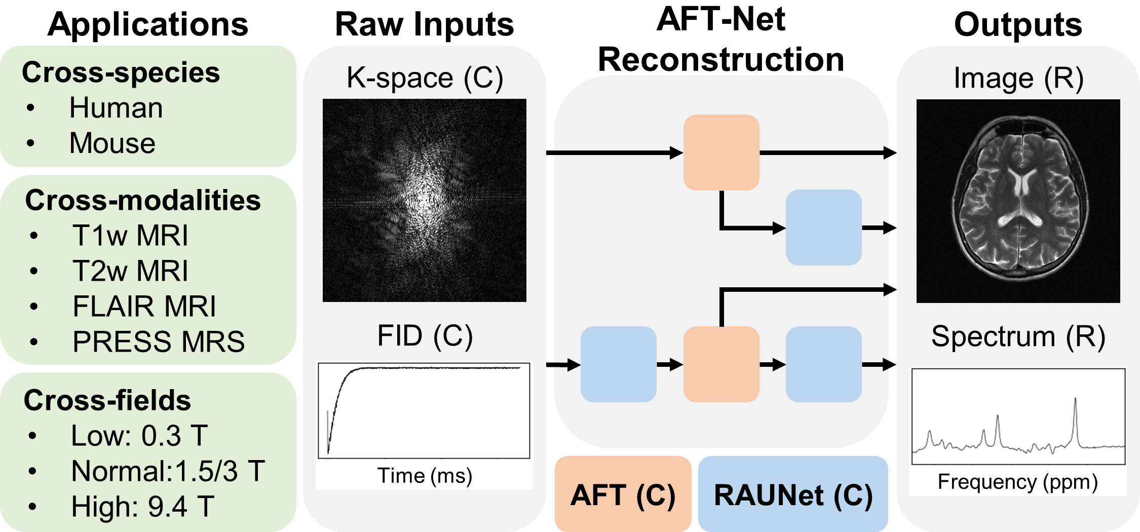
Figure 1: Schematics of general deep-learning MR imaging/spectroscopy reconstruction based on AFT-Net. The generality of AFT-Net is evaluated on the human normal-field MRI dataset (fastMRI [1]), human low-field MRI dataset (M4Raw [2]), mouse high-field MRI dataset (ours), and human normal-field MRI dataset (Big GABA [3]). The inputs of AFT-Net can be 2D MRI k-space data or 1D MRS FID data. The outputs are reconstructed MR images or spectra. Different structures of AFT-Net are developed by appending front-end and/or back-end convolutional layers to the AFT block. Here we show the human T2w 1.5T MRI and human 3T PRESS MRS reconstruction results, respectively. C: complex-valued and R: real-valued.

The domain shift from real coordinate space to complex coordinate space in the context of deep neural networks has uncovered the potential of utilizing the rich representational capacity of complex numbers and boosted the development of complex-valued neural architectures [4, 5, 6]. A similar but inverse domain shift is mirrored in the preprocessing of magnetic resonance imaging (MRI), where the raw data is acquired and stored in complex-valued k-space with each pixel representing the spatial frequency information in two or three dimensions of an object. Following the data acquisition, the raw k-space data is transformed into images that can be interpreted by the MR operator, physician, radiologist, or data scientist through the image reconstruction process, which shows to be an essential step in the preprocessing pipeline and lays the foundation for the overall image quality. Proper image reconstruction methods could increase the signal-to-noise ratio (SNR) by removing the thermal noise [7, 8], improve spatial inhomogeneous affected by point spread functions (PSFs), and fix unexpected signal artifacts [9].

Theoretically, image data is reconstructed by domain transforms (for example, Fourier transform, for fully sampled Cartesian data [10]. While under the setting of signal nonideality, which is normally presented in clinical acquisition, numerical and machine-learning methods are required where human experts are involved in selecting task-related features and establishing models that highly represent the mapping between the k-space domain and the image domain [11], including Fast Fourier Transform (FFT) [12], noise pre-whitening [9], digital signal processing (DSP), interpolation and coil combination. However, due to the significant variation in pathology and the possible oversight of human experts [13], a consistent and unbiased diagnosis cannot be guaranteed. In recent years, it has been shown that k-space, as a low-dimensional feature space, can be leveraged in deep neural networks to determine the between-manifold mapping of domain transforms in low signal-to-noise settings [14]. This image reconstruction process can be recast as a data-driven supervised learning task that determines the mapping between the k-space and image domains, which shows superior immunity to noise and reconstruction artifacts. The conventional discrete Fourier transform algorithm can be substituted by neural networks [15], which is derived mathematically and not based on learning. Thus, a fundamental neural network is presented that avoids the difficulties of network structure finding and algorithm optimization. A similar idea is adopted in domain-transform manifold learning in the phase-encoding direction [16] where front-end convolutional layers, intermediate global transform, and back-end convolutional layers are combined to perform data restoration in both k-space domain and image domain. Modern score-based diffusion models provide a powerful way to sample data from a conditional distribution given the measurements in the k-space domain, which can be used to solve inverse problems in imaging [17].

While most of the deep learning-based MR image reconstruction algorithms have applied the concept of domain-transform learning that directly learns a low-dimensional joint manifold between the k-space domain and the image domain, few works have fully leveraged the complex-valued neural network, which forces the neural network to implement learning-based frequency selection [18]. Some early works have proposed complex-valued neural networks (CVNNs) but mainly focus on solving the basics of learning [19, 20]. An extensive study on complex-valued CNNs has been conducted in recent years. A generalization of the real-valued CNN model has shown to be significantly less vulnerable to overfitting [5]. Mathematical argument and implementation are also discussed [21, 6], enabling the practical application of CVNNs. A combination of CVNNs and vision deep learning models (e.g. U-Net [22]) has recently emerged and is being exploited for MR image reconstruction [23, 24], demonstrating superior reconstruction and accelerated reconstruction compared to real-valued neural networks. However, the main drawback of previous CVNN works is that the potential of leveraging CVNN in domain-manifold learning is not fully investigated.

In this study, we combine domain-manifold learning with complex-valued neural networks to develop a unified end-to-end complex-valued image reconstruction approach for MRI. The framework we describe in this study is the artificial Fourier transform network (AFT-Net), as shown in Figure 1, which aims to get rid of any non-deep learning method in the preprocessing workflow and incorporate data processing into deep learning frameworks. It consists of trainable FC layers that approximate discrete Fourier transform (DFT) and complex-valued convolutional encoder-decoder networks to extract higher features in the k-space/image domain. Through the modular design, the proposed AFT-Net can be extended to any dimension (e.g. 1D MR spectroscopy data). We use the AFT-Net to accelerate/denoise MRI acquisition. In accelerated MRI reconstruction, the k-space data is under-sampled in the data acquisition direction (the phase-encoding direction). In denoised MRI reconstruction, a complex-valued Gaussian distribution is added to k-space data which approximates the thermal noise. We further applied the extended AFT-Net to denoised MRS acquisition, where the free induction decay (FID) data is under-sampled by decreasing repetition numbers. Comprehensive experiments are conducted under various species, modalities, system field strength, acceleration ratios, and noise levels.

In summary, AFT-Net incorporates domain-manifold learning and complex-valued neural networks with artificial Fourier transform blocks and convolutional encoder-decoder networks. The architecture learns the mapping between the k-space domain and the image domain while removing k-space/image artifacts through front-end/back-end convolutional networks. In the results section, we demonstrate that AFT-Net provides superior accelerated MRI reconstruction and denoised MRS reconstruction with an extended study under various datasets and low SNR settings.

2 Background

2.1 Complex-valued neural network

The definition of the conventional real-valued neural network can be extended to the complex domain. We denote a complex operator as $\mathrm{W}=\mathrm{W}_{real}+i\mathrm{W}_{imag}$, where $\mathrm{W}_{real}$ and $\mathrm{W}_{imag}$ are real-valued operators. The input complex vector can the represented as $x=x_{real}+ix_{imag}$. The output of complex operator $\mathrm{W}$ acting on $x$ is derived by multiplication:

$$\begin{split}y&=\mathrm{W}*x\\ &=(\mathrm{W}_{real}*x_{real}-\mathrm{W}_{imag}*x_{imag})\\ &+i(\mathrm{W}_{imag}*x_{real}+\mathrm{W}_{real}*x_{imag}).\end{split}$$ (1)

As the linear operator and convolution operator are distributive [6], we obtain:

$$\begin{split}\mathbb{C}\mathrm{Linear}(z)&=(\mathrm{Linear}_{1}(\Re(z))-\mathrm{Linear}_{2}(\Im(z)))\\ &+i(\mathrm{Linear}_{2}(\Re(z))+\mathrm{Linear}_{1}(\Im(z)))\end{split}$$ (2)

and

$$\begin{split}\mathbb{C}\mathrm{Conv}(z)&=(\mathrm{Conv}_{1}(\Re(z))-\mathrm{Conv}_{2}(\Im(z)))\\ &+i(\mathrm{Conv}_{2}(\Re(z))+\mathrm{Conv}_{1}(\Im(z)))\end{split}$$ (3)

where $z\in\mathbb{C}$ and we use subscripts $1$ and $2$ instead of $real$ and $imag$ to avoid misleading.

The complex version of the ReLU activation function we used in this study simply applies separate ReLU on both the real and the imaginary part of the input as follows:

$$\begin{split}\mathbb{C}\mathrm{ReLU}(z)&=\mathrm{ReLU}(\Re(z))+i\mathrm{ReLU}(\Im(z)))\end{split}$$ (4)

which satisfies Cauchy–Riemann equations when both the real and the imaginary parts have the same sign or $\theta_{z}\in[0,\frac{1}{2}\pi]\cup[\pi,\frac{3}{2}\pi]$.

Normalization is a common technique widely used in deep learning to accelerate training and reduce statistical covariance shift [25, 26, 27]. This is also mirrored in the complex-valued neural network, where we want to ensure that both the real and the imaginary parts have equal variance. Extending the normalization equation to matrix notation we have:

$$\tilde{z}=V^{-\frac{1}{2}}(z-\mathbb{E}(z))$$ (5)

where $x-\mathbb{E}(x)$ simply zero centers the real and the imaginary parts separately

$$z-\mathbb{E}(z)=\begin{bmatrix}\Re(z)-\mathrm{Mean}(\Re(z))\\ \Im(z)-\mathrm{Mean}(\Im(z))\end{bmatrix}$$ (6)

and $V$ is the covariance matrix

$$\begin{split}V&=\begin{bmatrix}V_{rr}&V_{ri}\\ V_{ir}&V_{ii}\end{bmatrix}+\epsilon I\\ &=\begin{bmatrix}\mathrm{Cov}(\Re(z),\Re(z))&\mathrm{Cov}(\Re(z),\Im(z))\\ \mathrm{Cov}(\Im(z),\Re(z))&\mathrm{Cov}(\Im(z),\Im(z))\end{bmatrix}+\epsilon I.\end{split}$$ (7)

$V$ is a $2\times 2$ matrix, and the existence of the inverse square root is guaranteed by the addition of $\epsilon I$ (Tikhonov regularization). Therefore, the solution of the inverse square root can be expressed analytically as

$$V=\begin{bmatrix}A&B\\ C&D\end{bmatrix}\Rightarrow V^{-\frac{1}{2}}=\begin{bmatrix}(D+s)/d&-B/d\\ -C/d&(A+s)/d\end{bmatrix}$$ (8)

where $s=\sqrt{AD-BC}$, $t=\sqrt{A+D+2s}$ and $d=st$.

The complex normalization is defined as

$$\mathrm{Norm}(z)=\gamma\tilde{z}+\beta=\begin{bmatrix}\gamma_{rr}&\gamma_{ri}\\ \gamma_{ri}&\gamma_{ii}\end{bmatrix}\tilde{z}+\begin{bmatrix}\Re(\beta)\\ \Im(\beta)\end{bmatrix}.$$ (9)

Considering the limitation of GPU RAM and large memory consumption of complex-valued networks, we use the complex group normalization in our framework to avoid possible inaccurate batch statistics estimation caused by a small batch size.

Algorithm 1 Complex group normalization

Input: $z$, $\gamma$, $\beta$, $G$ (number of groups), $\epsilon$

Shape of $z$ is $(B,C,H,W)$

Reshape $z$ to $(B,G,C//G,H,W)$

for each group do

     $\tilde{z}\leftarrow V^{-\frac{1}{2}}(z-\mathbb{E}(z))$ based on Equations 6, 7 and 8.

end for

Reshape $\tilde{z}$ to $(B,C,H,W)$

return $\gamma\tilde{z}+\beta$

3 Methods

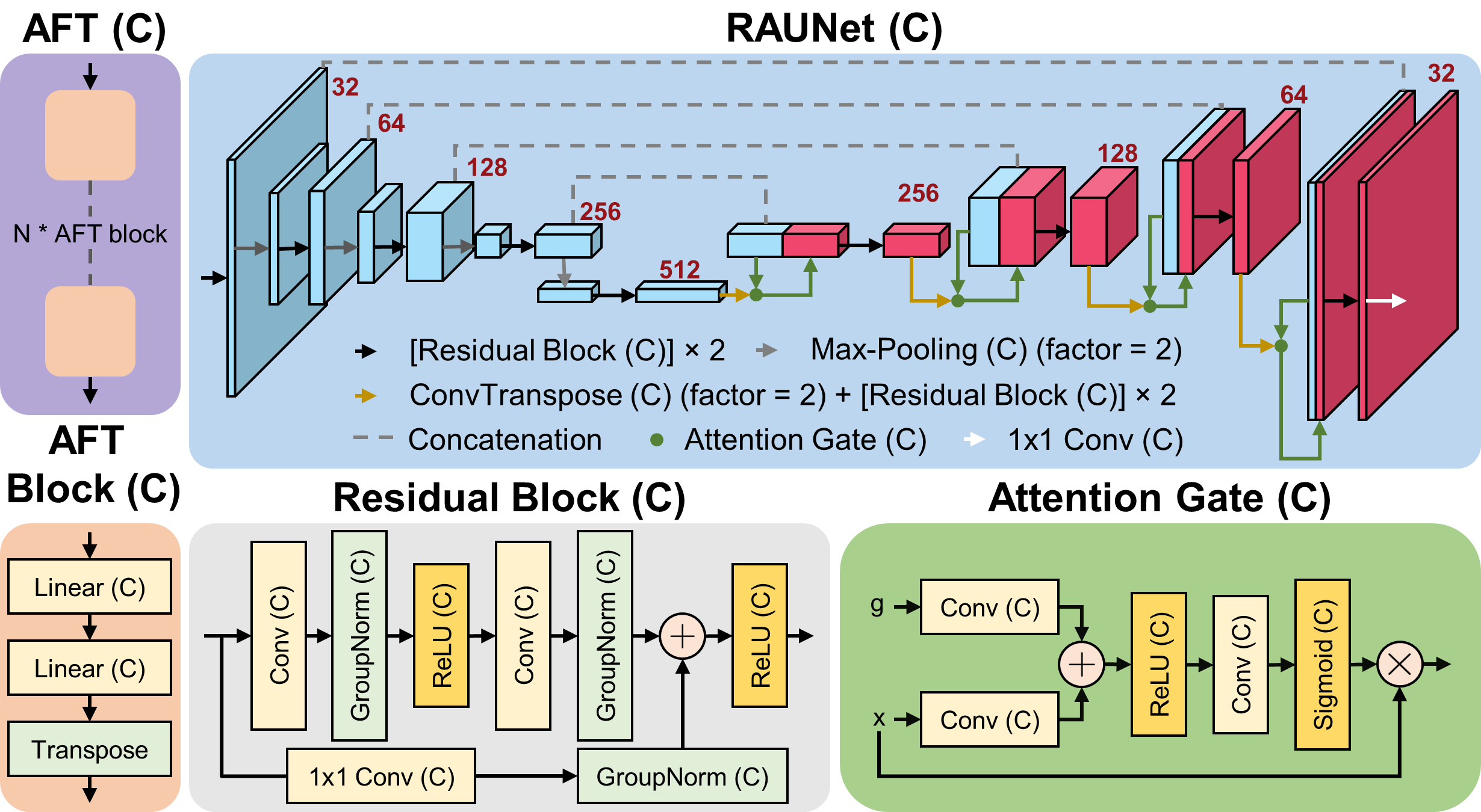
Figure 2: Structure of N-dimensional AFT-Net (N can be 1, 2, or 3). Components include the complex-valued AFT block, the complex-valued residual attention U-Net, the complex-valued residual block, and the complex-valued attention gate. All convolutional layers have a kernel size of 3, except those pointed out specifically. C: complex-valued. Red numbers indicate the number of channels produced by each layer.

3.1 Artificial Fourier Transform

Since 2D discrete Fourier transform (DFT) is a linear operation and can be represented by two successive 1D DFTs as

$$\begin{split}\mathcal{F}_{x,y}\{f(x,y)\}&=\mathcal{F}_{x}\{\mathcal{F}_{y}\{f(x,y)\}\}\\ &=\mathcal{F}_{y}\{\mathcal{F}_{x}\{f(x,y)\}\},\end{split}$$ (10)

each dimension of 2D DFT can be modeled as a single-hidden-layer neural network with a linear activation function[15]. We further implemented this idea with complex-valued neural networks and proposed AFT with two repeated blocks. Each block consists of two complex linear layers followed by a transpose operation as shown in Figure 2.

From the definition of the discrete Fourier transform of a sequence of $N$ complex numbers which can be represented in the real and imaginary parts as

$$Z_{k}=\sum_{n=0}^{N-1}z_{n}\left[\cos\left(\frac{2\pi}{N}kn\right)-i\sin\left(\frac{2\pi}{N}kn\right)\right],$$ (11)

rewrite Equation 11 as

$$Z_{k}=W_{real}z+iW_{imag}z,$$ (12)

where $W_{real}$ and $W_{imag}$ are the real and the imaginary coefficients. Use matrix notation to represent real and imaginary parts of the DFT operation. We have:

$$\begin{bmatrix}\Re(Z_{k})\\ \Im(Z_{k})\end{bmatrix}=\begin{bmatrix}W_{real}&-W_{imag}\\ W_{imag}&W_{real}\end{bmatrix}\begin{bmatrix}\Re(z)\\ \Im(z)\end{bmatrix}.$$ (13)

Compare Equation 13 with Equation 1, a multi-layer complex-valued neural network with linear activation function can represent 1D DFT with appropriate weights. We use $AFT_{N}$ to denote the complex-valued Fourier transform deep learning block on the input vector with $N$ elements. The Fourier transform of the input data with dimension $H\times W$ can be represented as

$$Z=\mathrm{AFT}_{H}(\mathrm{AFT}_{W}(z)^{\intercal})^{\intercal}.$$ (14)

3.2 Network framework

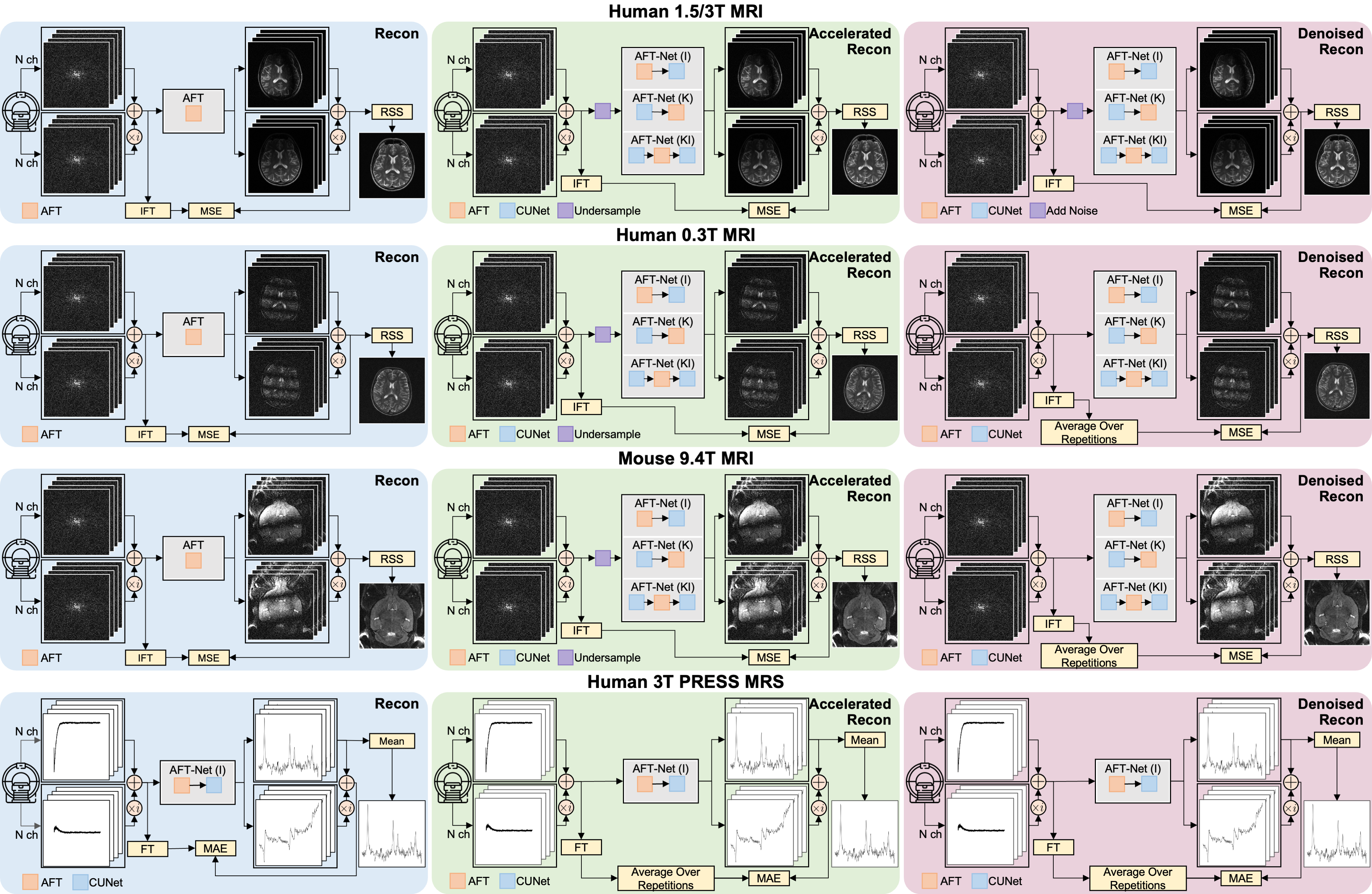
Figure 3: The workflows of experiments on each dataset.

The network structure and general workflow are shown in Figure 2 and Figure 3. We apply our AFT to the multi-coil k-space data acquired directly from the scanner for the reconstruction task. The target is derived from the inverse fast Fourier transform on the input data. The AFT does not compress the coil channel so that the input and output shapes/sizes are the same. The network performance is evaluated within magnitude images obtained by the Fourier application and coil compression. For the reconstruction plus denoising task, we combine our AFT with an entirely complex-valued U-Net [23], which extracts higher features in the k-space and/or image domain and forces the network to represent sparsely in those domains. Multiple network architectures are evaluated to verify the effectiveness of both AFT and CUNet in different domains. We refer each of them to AFT, AFT-Net (I), AFT-Net (K), and AFT-Net (KI), respectively as shown in Figure 3. We first train an AFT-only network to see if, without a non-linear activation function, the AFT can remove noise and enhance quality. Then a network with the AFT followed by the CUNet is trained to simulate a typical deep learning workflow where conventional numerical methods are used to preprocess the image, and CNNs are utilized to map the input domain to the target domain. We also evaluate the network with CUNet first implemented directly on the k-space domain. Given that each position in k-space contains the information of the whole image, CNNs implemented in k-space can leverage the complete information of all space, even if they have a fixed field of view. Finally, a CUNet-AFT-CUNet structure is evaluated with the first CUNet extracts k-space domain features and the second CUNet extracts image domain features.

The architecture of the CUNet presented in Figure 2 is generally based on the residual attention U-Net but with all the real-valued components replaced by complex-valued components as shown in Figure 2, including complex-valued convolutional layers and complex-valued ReLU layers introduced in Section 2.1. We further optimize the network for smaller batch sizes by replacing batch normalization with group normalization. Other complex components are implemented in the same way. For example, the complex transposed convolution operator can be mirrored from Equation 3, complex sigmoid is applied like complex ReLU, and complex max pooling is almost the same as the real-valued version with indices inferred from absolute values.

3.3 Implementation details

We construct a batch size of 1 and optimize the network using the ADAM[28] optimizer. The initial learning rate is set to $10^{-3}$, and we used a learning rate scheduler based on the SSIM in the validation set. When the metric has stopped improving, the learning rate is reduced by a factor of $\sqrt{10}$. We set patience to 2 and the lower bound of the learning rate to $10^{-6}$. The training will stop early once learning stagnates and the learning rate reaches the lower bound. All experiments are done using PyTorch 1.11.0 and a Quadro RTX 6000 GPU.

In the context of image reconstruction and processing, the impact of the loss function is vital if the final results are to be evaluated by human observers. One common and safe choice is $\ell_{2}$ loss which works under the assumption of white Gaussian noise. For training AFT for MRI reconstruction, the loss value is determined in the frequency domain as

$$\mathcal{L}^{recon}=\mathcal{L}^{\ell_{2}}(\Re(x),\Re(y))+\mathcal{L}^{\ell_{2}}(\Im(x),\Im(y))$$ (15)

so that both real and imaginary outputs are optimized to match the conventional Fourier transformation. For training AFT-Net for accelerated MRI reconstruction, we only want to minimize the error of magnitude images. Therefore, the loss value for accelerated MRI reconstruction is determined in the image domain after coil combination. The root-sum-of-squares (RSS) approach [29] is applied to complex-valued output from the model to generate to optimal, unbiased estimate of magnitude image which is used for loss calculation.

3.4 Experimental data

Three brain MRI datasets and one brain MRS dataset were used in this study: a complex-valued normal-field human brain MRI dataset from the fastMRI dataset [1], a complex-valued low-field human brain MRI dataset from the [2], a complex-valued high-field mouse brain dataset from our lab (Small Animal Imaging Lab, Zuckerman Institute, Columbia University), a complex-valued human brain MRS dataset from the Big GABA dataset [3]. The proposed methods were trained on these datasets separately.

The normal-field human brain MRI dataset contains fully sampled brain MRIs obtained on 3 and 1.5 Tesla magnets. We selected 4-channels axial T1-weighted and T2-weighted scans from the raw fastMRI dataset. A total number of 993 scans were used with 794, 99, and 100 each for the training, validation, and test set. All the scans were first normalized to the max intensity value of one and cropped to $640\times 320$ matrix size.

The low-field human brain MRI dataset contains fully sampled brain MRIs obtained on 0.3 Tesla magnets. We selected 4-channels axial T1-weighted, T2-weighted, and FLAIR scans from the raw M4Raw dataset. A total number of 1264 scans were used with 1024, 122, and 118 each for the training, validation, and test set. All the scans were first normalized to the max intensity value of one and cropped to $256\times 256$ matrix size.

The high-field mouse brain MRI dataset contains fully sampled brain MRIs obtained on 9.4 Tesla magnets using the Bruker Biospec 94/30 scanner and ParaVision 6.0.1. Each subject was scanned for 4 repetitions with a 4-channel CryoProbe. A total number of 960 scans were acquired from 240 subjects with 192, 24, and 24 each for the training, validation, and test set. All the scans were first normalized to the max intensity value of one and cropped to $416\times 224$ matrix size.

The human brain MRS dataset contains GABA-edited MEGA-PRESS data obtained on 3T Philips scanners from different sites. Each subject was scanned for 320 averages (160 ON and 160 OFF repetitions). The data points acquired by each repetition is 2048. A total number of 101 scans were selected from the Big GABA dataset with 80, 10, and 11 each for the training, validation, and test set. All the scans were first normalized to the max spectra magnitude value of one.

During the accelerated MRI reconstruction, all the k-space data was undersampled from the fully sampled k-space by applying a mask in the phase-encoding direction. We use the acceleration rate (or acceleration factor), to denote the level of scan time reduced for the undersampled k-space data, which is defined as the ratio of the amount of k-space data required for a fully sampled image to the amount collected in an undersampled k-space data [30]. The sampling ratio, SR, is also used to denote the information retained in the undersampled k-space data, which is defined as the inverse of the acceleration rate. An equispaced mask with approximate acceleration matching is used to undersample the k-space data. The fraction of low-frequency columns to be retained for acceleration rates 2x, 4x, 8x, and 16x are 16%, 8%, 4%, and 2% respectively.

During the denoised MRI reconstruction, complex-valued Gaussian noise is added to the k-space data with different levels. For the human normal-field MRI dataset, the standard deviation (or scale) was chosen to be 0.005, 0.01, and 0.02. For the human low-field MRI dataset, the scale was chosen to be 4.8. For the mouse high-field MRI dataset, the noisy scans could be chosen to be a single repetition or manually added Gaussian noise with a scale of 0.4.

During the denoised MRS reconstruction, we use the reduction rate, R, to denote the noise level, which is defined as the ratio of the number of total repetitions (160 for this study) to the number of repetitions retained for a noisy input. We generate the noisy FIDs with 5 reduction rates of 10, 20, 40, 80, and 160.

3.5 Measurement of Reconstruction Quality

Three metrics were adopted for the quantitative evaluation of the image quality compared with the ground truth: structural similarity (SSIM) [31], peak signal-to-noise ratio (PSNR), and normalized root mean squared error (NRMSE). For the quality measurement of the 1D spectra, another three metrics were used: Pearson correlation coefficient (PCC), Spearman’s rank correlation coefficient (SCC), and goodness-fitting coefficient (GFC) [32]. The GFC is introduced to evaluate the goodness of the mathematical reconstruction with a value ranging from 0 to 1, where 1 indicates a perfect reconstruction. If $\hat{y}_{i}$ is the predicted value of the $i$-th sample and $y_{i}$ is the corresponding true value, then the GFC estimated over $n_{\text{samples}}$ is defined as

$$\text{GFC}(y,\hat{y})=\frac{|\sum_{i=0}^{n_{\text{samples}}-1}y_{i}\hat{y}_{i}|}{|\sum_{i=0}^{n_{\text{samples}}-1}y_{i}^{2}|^{1/2}|\sum_{i=0}^{n_{\text{samples}}-1}\hat{y}_{i}^{2}|^{1/2}}.$$ (16)

4 Results

4.1 Comparison of score-MRI and AFT-Net

Metrics	Zero Filling	score-MRI	AFT-Net (KI)
SSIM	0.747 ± 0.033	0.853 ± 0.022	0.895 ± 0.027 (****)
PSNR (dB)	27.2 ± 1.8	30.2 ± 1.8	32.2 ± 1.6 (****)
NRMSE	0.203 ± 0.039	0.143 ± 0.029	0.113 ± 0.026 (****)

Table 1: Comparison between score-MRI and AFT-Net (KI) in terms of SSIM, PSNR, and NRMSE. Numbers are presented as mean value ± standard deviation. p-values indicate results from two-sided t-tests for paired samples. (ns: $p>0.05$, *: $p\leq 0.05$, **: $p\leq 0.01$, ***: $p\leq 0.001$, ****: $p\leq 0.0001$)

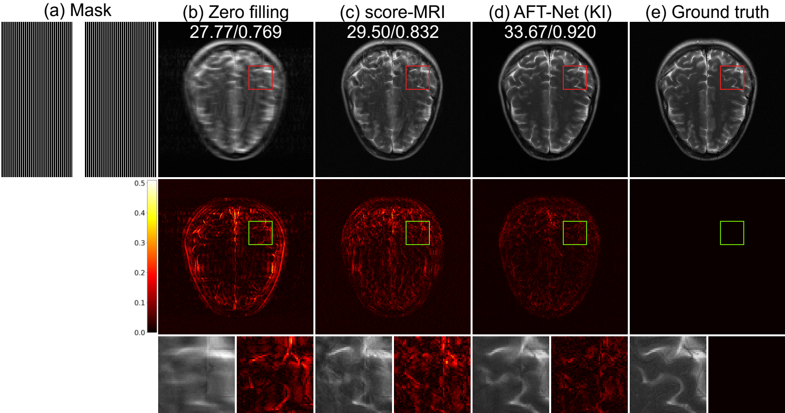
Figure 4: Comparison between score-MRI and AFT-Net. (a) The sub-sampling mask used to generate the under-sampled image, (b) zero filling, (c) score-MRI, (d) AFT-Net (KI), and (e) ground truth. 1st row: 1D 4x equal-spaced sampling (8% of low-frequency columns are retained), 2nd row: difference magnitude against (e) (in Hot colormap), 3rd row: zoomed-in version of the indicated box in 1st row and 2nd row. White numbers in the upper center location indicate PSNR (dB), and SSIM, respectively.

The effectiveness of the AFT-Net was evaluated through a comparative study. We compare the performance of AFT-Net (KI) with score-MRI, which solves the image reconstruction inverse problem based on score-based generative models. The score-MRI does not incorporate a complex-valued neural network to calculate the score function. Because the score-MRI iterates between the numerical SDE solver and data consistency step to achieve reconstruction at the inference stage which takes 3h for each image, we evaluate the models over a subset of the human normal-field MRI dataset with 445 images. The quantitative metrics demonstrate the superior performance of AFT-Net over score-MRI, as shown in Table 1, including the mean ± standard deviation of SSIM, PSNR, and NRMSE values. The statistical t-test between the metrics of score-MRI and AFT-Net also shows the superior accelerated reconstruction of the proposed method with a p-value under 0.0001. Qualitatively, AFT-Net outperformed score-MRI, as can be seen from the difference magnitude map and zoomed-in area in Figure 4.

4.2 Generality of AFT-Net

Different structures of AFT-Net, as mentioned in Section 3.2, were compared under various MRI datasets with different field strengths, different species, and different modalities to verify the stability and generality of the AFT-Net. In addition, the effectiveness of the front-end/back-end convolutional networks is also evaluated in this section. To validate the robustness of AFT-Net to k-space artifacts, these proposed AFT-Net structures were compared on the image reconstruction, accelerated reconstruction, and denoised reconstruction as described in Section 3.4. Furthermore, the extended AFT-Net was compared with numerical methods using 1-dimensional MRS FID data on the denoised reconstruction.

4.2.1 Human normal-field MRI study

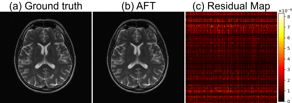
Figure 5: Human 1.5/3T MRI reconstruction results. (a) Ground truth, (b) proposed method, (c) difference magnitude of (a) and (b) (in Hot colormap).

First, we show the results of human 1.5/3T MRI reconstruction using raw fully-sampled fastMRI k-space data in Figure 5. All the images shown here and in the following sections are cropped so that the anti-aliasing placed outside the field of view (FOV) in phase-encoding directions is removed. The ground truth image is derived by applying conventional Fourier transformation to the k-space data. It can be seen that the ground truth image obtained from FT is identical to the AFT prediction, which human observers can not distinguish. The results adhere to the mathematical description we discussed in Section 2.1. The residual map (pixel-wise difference between the ground truth image and the AFT prediction) shows that no brain structural information is presented. The grid-like remaining error is mainly caused by precision loss during floating-point calculation in matrix multiplication.

In LABEL:fig:4211_fastMRI_acc_recon, we show the results of human 1.5/3T accelerated reconstruction using under-sampled fastMRI k-space data. In the first row, we see the reconstructions from 1D 4x equal-spaced sampling, in which 8% of low-frequency columns are retained. Here, we compare different AFT-Net structures with the zero-filling method. AFT-Net (KI) performs outstanding reconstruction, where less structural difference can be seen from the residual map in the second row. The third row shows zoomed-in areas of both images and residual maps. AFT-Net (I) produces a more blurry reconstruction which loses the structural details. Reconstruction through AFT-Net (K) induces foggy artifacts, which is reflected in terms of SSIM. LABEL:fig:4212_fastMRI_acc_recon_box1 shows the accelerated reconstruction results by comparing AFT-Net (I, K, and KI) and zero filling in terms of SSIM across acceleration rates 2x, 4x, 8x, and 16x. The performance of zero filling drops linearly as the acceleration rate increases while the AFT-Net methods are more robust to the acceleration scale. The t-test between each AFT-Net structure indicates that the AFT-Net (KI) overcomes all other AFT-Net structures significantly. The results of AFT-Net on different acquisition types and system field strength in LABEL:fig:4213_fastMRI_acc_recon_box2 demonstrate that AFT-Net is robust to contrast difference and image quality.

Next, we illustrate the results of human 1.5/3T denoised reconstruction using fastMRI k-space data with added Gaussian noise in LABEL:fig:4214_fastMRI_denoise_recon. Unlike the results of accelerated reconstruction, AFT-Net (I) performs the best across all three proposed AFT-Net structures, which can be proved from the t-test results in LABEL:fig:4215_fastMRI_denoise_recon_box1. It is also demonstrated in LABEL:fig:4215_fastMRI_denoise_recon_box1 that AFT-Net (KI) only shows comparable performance against AFT-Net (K) when the noise scale is 0.02 and underperforms other AFT-Net structures in noise scale 0.005 and 0.01, indicating that increasing the depth of AFT-Net does not necessarily increase the overall performance especially for denoised reconstruction task. The second row shows the pixel-wise difference between AFT-Net output and noiseless ground truth. It can be indicated that the noise in the background is attenuated significantly. Although the brain structure can be seen from the residual map, the zoomed-in version of the image shows that the AFT-Net reconstruction preserves the anatomy structure. The results of AFT-Net on different acquisition types and system field strength in LABEL:fig:4216_fastMRI_denoise_recon_box2 also demonstrate the generality of AFT-Net against different imaging modalities.

A comprehensive comparison of quantitative metrics on the test set is provided in LABEL:tab:fastMRI_recon, LABEL:tab:fastMRI_acc_recon and LABEL:tab:fastMRI_denoise_recon for reconstruction, accelerated reconstruction, and denoised reconstruction accordingly. AFT-Net (KI) significantly outperforms other AFT-Net structures on all the different acceleration rates. On all the different noise scales, AFT-Net (I) performs significantly better than other AFT-Net structures. More detailed quantitative metrics of human 1.5/3T MRI accelerated reconstruction and denoised reconstruction results are provided in the appendix, which is grouped by image contrast and system field strength.

It is worth mentioning that although AFT-Net (K) does not outperform other AFT-Net structures in both accelerated reconstruction and denoised reconstruction tasks, it demonstrates the ability to learn in a sparse frequency domain and its sparse representations with a complex-valued convolutional network.

4.2.2 Human low-field MRI study

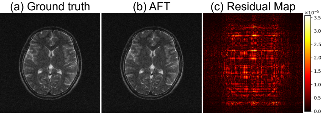
Figure 6: Human 0.3T MRI reconstruction results. (a) Ground truth, (b) proposed method, (c) difference magnitude of (a) and (b) (in Hot colormap).

First, we show above the results of human 0.3T MRI reconstruction using raw fully-sampled M4Raw k-space data in Figure 6. All images were processed at the size of 256 x 256, with phase encoding in the X (LR) direction, and no cropping or reshaping was done due to it having been done already by the original M4Raw authors. The ground truth image was derived from the raw k-space data using a conventional Fourier transform method. From the image, we note that the image generated by AFT-Net is essentially identical to the Ground Truth. The results adhere to the mathematical description discussed in Section 2.1. The residual map shows minor brain structural information around the edges of the brain. Most of the remaining grid error is from floating point errors during matrix multiplication.

In LABEL:fig:4221_M4Raw_acc_recon, we show the results of human 0.3T accelerated reconstruction using under-sampled M4Raw k-space data. In the first row, we see the reconstructions from 1D 4x equal-spaced sampling, in which 8% of low-frequency columns are retained. We compare different AFT-Net structures against the Zero-Filling method. AFT-Net (KI) performs the best reconstruction, where the least structural difference can be seen from the residual map in the second row. The third row shows zoomed-in areas of both images and residual maps. AFT-Net (K) produces a more blurry reconstruction which loses the structural details. Reconstruction through AFT-Net (I) produces somewhat similar results to AFT-Net (KI) but loses some structural detail. LABEL:fig:4222_M4Raw_acc_recon_box1 shows the accelerated reconstruction results by comparing AFT-Net (I, K and KI) and zero filling in terms of SSIM across acceleration rates 2x, 4x, 8x and 16x. The performance of zero filling drops linearly as the acceleration rate increases while the AFT-Net methods are more robust to the acceleration scale. The t-test between each AFT-Net structure indicates that the AFT-Net (KI) clearly performs better than all other AFT-Net structures. The results of AFT-Net on different acquisition types and system field strength in LABEL:fig:4223_M4Raw_acc_recon_box2 demonstrate that AFT-Net performs better on T1w images at 0.3T, but is robust in terms of image quality and retains excellent performance on other contrasts.

Next, we illustrate the results of human 0.3T denoised reconstruction using M4Raw k-space data with added Gaussian noise in LABEL:fig:4224_M4Raw_denoise_recon at a scale of 4.8. The noise scale was determined using the averaged maximum values of the dataset to stay in line with noise scales used for 1.5/3T tests. Unlike the results of accelerated reconstruction, AFT-Net (I) performs slightly better among three proposed AFT-Net structures, which can be seen in the t-test results in LABEL:fig:4225_M4Raw_denoise_recon_box1. Note that AFT-Net (I) does not hold a very significant advantage in SSIM, PSNR, or NRMSE compared to AFT-Net (KI) as demonstrated in LABEL:tab:M4Raw_denoise_recon. The second row shows the pixel-wise difference between AFT-Net output and noiseless ground truth. It can be indicated that the noise in the background is attenuated significantly. Although the brain structure can be seen from the residual map, the zoomed-in version of the image shows that the AFT-Net reconstruction preserves the anatomical structure. The results of AFT-Net on different acquisition types and system field strength in LABEL:fig:4226_M4Raw_denoise_recon_box2 also demonstrate that AFT-Net performs better on T1w images at 0.3T, but has good generality against different imaging modalities.

A comprehensive comparison of quantitative metrics on the test set is provided in LABEL:tab:M4Raw_recon, LABEL:tab:M4Raw_acc_recon and LABEL:tab:M4Raw_denoise_recon for reconstruction, accelerated reconstruction and denoised reconstruction accordingly. AFT-Net (KI) significantly outperforms other AFT-Net structures on all the different acceleration rates. On denoised reconstruction, AFT-Net (I) performs slightly better than other AFT-Net structures. More detailed quantitative metrics of human 0.3T MRI accelerated reconstruction and denoised reconstruction results are provided in the appendix, which is grouped by image contrast and system field strength.

It is worth mentioning that although AFT-Net (K) does not outperform other AFT-Net structures in both accelerated reconstruction and denoised reconstruction tasks, it demonstrates the ability to learn in a sparse frequency domain and its sparse representations with a complex-valued convolutional network.

4.2.3 Mouse high-field MRI study

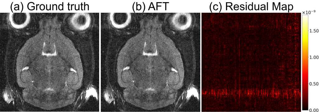
Figure 7: Mouse 9.4T MRI reconstruction results. (a) Ground truth, (b) proposed method, (c) difference magnitude of (a) and (b) (in Hot colormap).

First, we show the results of mouse 9.4T MRI reconstruction using fully-sampled k-space data acquired with a Bruker Biospec 94/30 scanner in Figure 7. The scanner is equipped with state-of-the-art MRI imaging RF coils, including a 1H mouse-head-only Cryogenic RF coil designed for boosted signal sensitivity with a proven factor at 3̃ for in vivo brain imaging. The reconstructed images are cropped so that the anti-aliasing placed outside the field of view (FOV) in phase-encoding directions is removed. The residual map (pixel-wise difference between the ground truth image and the AFT prediction) shows that no brain structural information is presented. The grid-like remaining error is mainly caused by precision loss during floating-point calculation in matrix multiplication.

In Figure 8, we show the results of mouse 9.4T accelerated reconstruction using under-sampled mouse MRI k-space data. In the first row, we see the reconstructions from 1D 4x equal-spaced sampling, in which 8% of low-frequency columns are retained. We compare different AFT-Net structures against the Zero-Filling method. AFT-Net (KI) performs the best reconstruction, where the least structural difference can be seen from the residual map in the second row. The third row shows zoomed-in areas of both images and residual maps. AFT-Net (K) produces a more blurry reconstruction which loses the structural details. Reconstruction through AFT-Net (I) produces somewhat similar results to AFT-Net (KI) but loses some structural detail. Figure 9 shows the accelerated reconstruction results by comparing AFT-Net (I, K, and KI) and zero filling in terms of SSIM across acceleration rates 2x, 4x, 8x, and 16x. The performance of zero filling drops linearly as the acceleration rate increases while the AFT-Net methods are more robust to the acceleration scale. The t-test between each AFT-Net structure indicates that the AFT-Net (KI) performs better than all other AFT-Net structures.

Next, we illustrate the results of mouse 9.4T denoised reconstruction using mouse MRI k-space data with added Gaussian noise in Figure 10 at a scale of 0.8. Unlike the results of accelerated reconstruction, AFT-Net (I) performs slightly better among three proposed AFT-Net structures, which can be seen in the t-test results in Figure 11. Note that AFT-Net (I) does not hold a very significant advantage in SSIM, PSNR, or NRMSE compared to AFT-Net (KI) as demonstrated in Table 3. The second row shows the pixel-wise difference between AFT-Net output and noiseless ground truth. It can be indicated that the noise in the background is attenuated significantly. Although the brain structure can be seen from the residual map, the zoomed-in version of the image shows that the AFT-Net reconstruction preserves the anatomical structure.

A comprehensive comparison of quantitative metrics on the test set is provided in Table 2 and Table 3 for accelerated reconstruction and denoised reconstruction accordingly. AFT-Net (KI) significantly outperforms other AFT-Net structures on all the different acceleration rates. On denoised reconstruction, AFT-Net (I) performs slightly better than other AFT-Net structures.

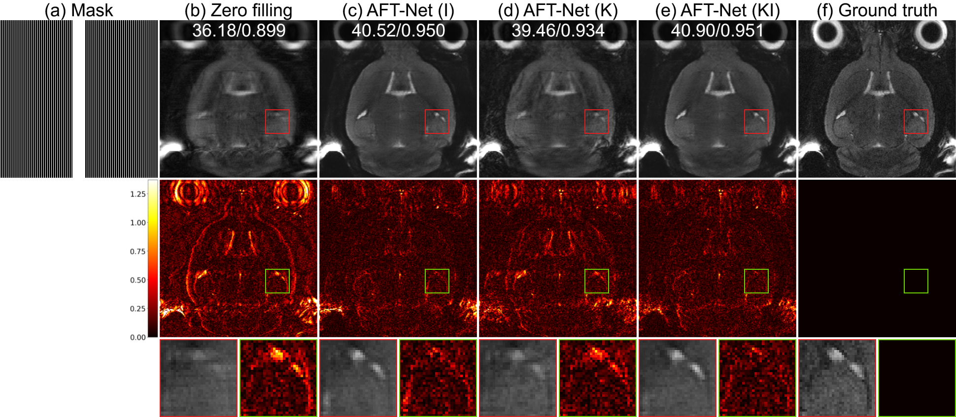
Figure 8: Mouse 9.4T MRI accelerated reconstruction results. (a) Sub-sampling mask used to generate under-sampled image, (b) zero filling, (c)-(e) proposed methods, and (f) ground truth. 1st row: 1D 4x equal-spaced sampling (8% of low-frequency columns are retained), 2nd row: difference magnitude against (f) (in Hot colormap), 3rd row: zoomed-in version of the indicated box in 1st row and 2nd row. White numbers in the upper center location indicate PSNR (dB), and SSIM, respectively.

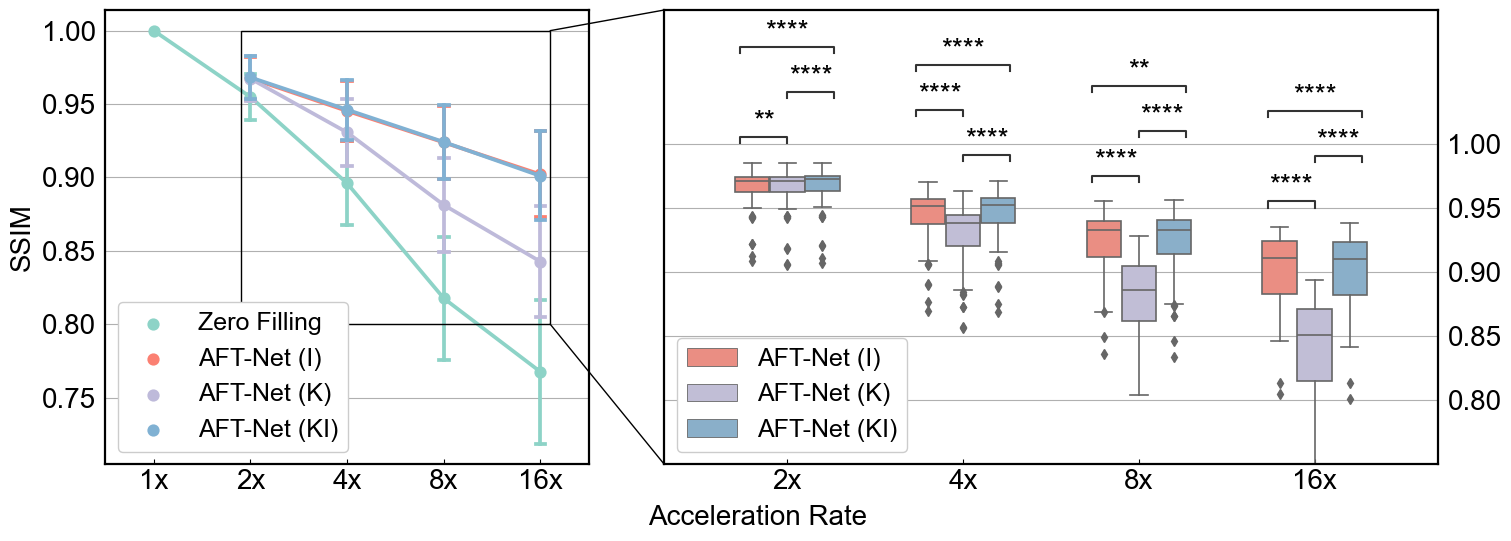
Figure 9: Results of mouse 9.4T MRI accelerated reconstruction by comparing AFT-Net (I Model, K Model, and KI Model) in terms of SSIM, PSNR, and NRMSE. p-values indicate results from two-sided t-tests for paired samples. (ns: $p>0.05$, *: $p\leq 0.05$, **: $p\leq 0.01$, ***: $p\leq 0.001$, ****: $p\leq 0.0001$)

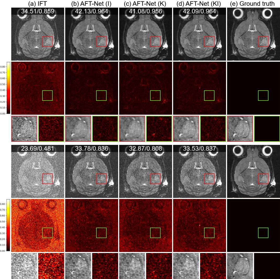
Figure 10: Mouse 9.4T MRI denoised reconstruction results. (a) Input, (b)-(d) proposed methods, and (e) ground truth. 1st row: Single repetition denoise, 4th row: Randomly added Gaussian noise in k-space (scale = 0.4), 2nd and 5th row: difference magnitude against (e) (in Hot colormap), 3rd and 6th row: zoomed-in version of the indicated box in 1st row and 2nd row. White numbers in the upper center location indicate PSNR (dB), and SSIM, respectively.

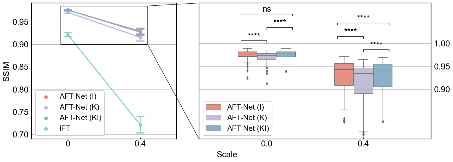
Figure 11: Results of mouse 9.4T MRI denoised reconstruction by comparing AFT-Net (I Model, K Model, and KI Model) in terms of SSIM, PSNR, and NRMSE. p-values indicate results from two-sided t-tests for paired samples. (ns: $p>0.05$, *: $p\leq 0.05$, **: $p\leq 0.01$, ***: $p\leq 0.001$, ****: $p\leq 0.0001$)

			AFT-Net
Acceleration Rate	Metrics	Zero Filling	I Model	K Model	KI Model
2x (SR = 50%)	SSIM	0.955 ± 0.016	0.968 ± 0.014	0.967 ± 0.015	0.968 ± 0.015
	PSNR (dB)	40.7 ± 2.0	43.1 ± 2.1	43.3 ± 2.1	43.3 ± 2.1
	NRMSE	0.162 ± 0.016	0.123 ± 0.012	0.122 ± 0.014	0.121 ± 0.013
4x (SR = 25%)	SSIM	0.896 ± 0.029	0.945 ± 0.020	0.931 ± 0.023	0.946 ± 0.020
	PSNR (dB)	36.1 ± 1.9	40.3 ± 1.9	39.3 ± 1.9	40.6 ± 1.9
	NRMSE	0.276 ± 0.015	0.170 ± 0.009	0.192 ± 0.011	0.165 ± 0.010
8x (SR = 12.5%)	SSIM	0.818 ± 0.042	0.924 ± 0.025	0.881 ± 0.032	0.924 ± 0.025
	PSNR (dB)	32.8 ± 1.8	38.3 ± 1.8	35.9 ± 1.8	38.5 ± 1.8
	NRMSE	0.403 ± 0.019	0.214 ± 0.017	0.284 ± 0.022	0.211 ± 0.016
16x (SR = 6.25%)	SSIM	0.767 ± 0.049	0.902 ± 0.029	0.843 ± 0.038	0.901 ± 0.030
	PSNR (dB)	31.1 ± 1.8	36.8 ± 1.8	34.1 ± 1.8	36.9 ± 1.8
	NRMSE	0.489 ± 0.028	0.257 ± 0.027	0.349 ± 0.032	0.253 ± 0.024

Table 2: Quantitative metrics of mouse 9.4T MRI accelerated reconstruction and evaluation on the dataset with various acceleration rates. Numbers are presented as mean value ± standard deviation. Numbers in boldface indicate the lowest NRMSE and the highest PSNR/SSIM values.

			AFT-Net
		IFT	I Model	K Model	KI Model
T2w	SSIM	0.921 ± 0.024	0.976 ± 0.010	0.971 ± 0.011	0.976 ± 0.009
	PSNR (dB)	38.2 ± 2.0	43.8 ± 2.2	42.7 ± 2.0	43.7 ± 2.2
	NRMSE	0.211 ± 0.041	0.112 ± 0.025	0.126 ± 0.023	0.112 ± 0.024
T2w with	SSIM	0.722 ± 0.097	0.929 ± 0.036	0.915 ± 0.042	0.927 ± 0.036
added noise	PSNR (dB)	29.9 ± 3.0	39.2 ± 2.8	38.3 ± 2.8	38.9 ± 2.8
	NRMSE	0.564 ± 0.179	0.192 ± 0.053	0.214 ± 0.059	0.198 ± 0.055

Table 3: Quantitative metrics of mouse 9.4T MRI denoised reconstruction and evaluation on the dataset with added Gaussian noise (scale = 0.4). Numbers are presented as mean value ± standard deviation. Numbers in boldface indicate a significant difference against all other metrics, derived from paired two-sample t-tests under the null hypothesis.

4.2.4 Human normal-field MRS study

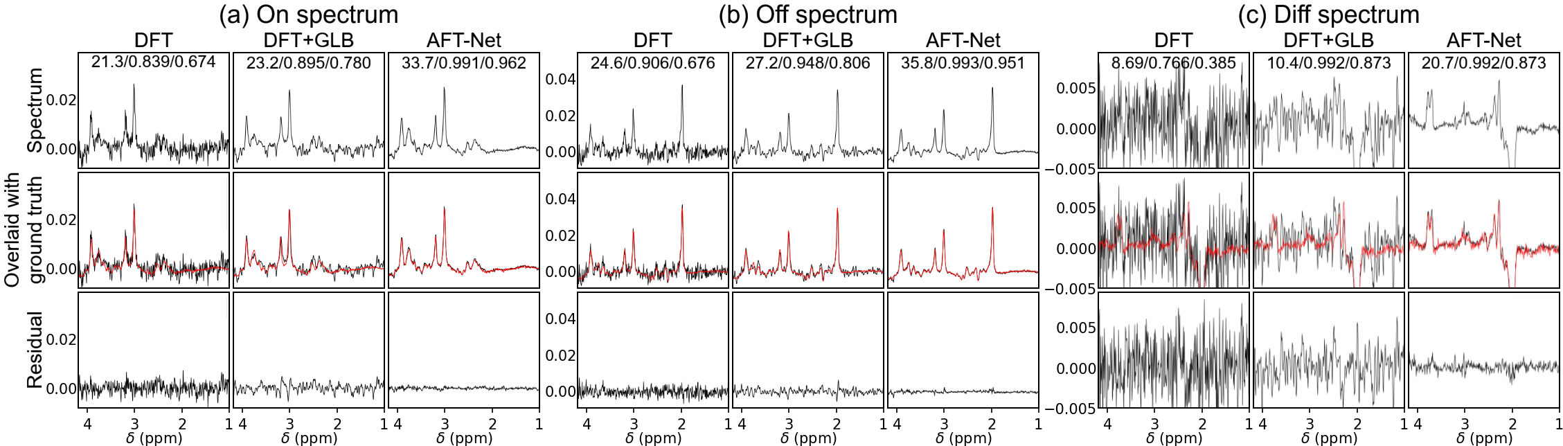
Figure 12: Human 3T MRS denoised reconstruction results. The acceleration rate is 80 for each spectrum. (a) Reconstruction results for the ON spectrum, (b) reconstruction results for the OFF spectrum, and (c) results for the DIFF spectrum derived from (a) and (b). 1st row: reconstructed spectra, 2nd row: reconstructed spectra overlaid with ground truth (in red line), 3rd row: Difference of reconstructed spectra against ground truth. Black numbers in the upper center location indicate PSNR (db), PCC, and SCC, respectively.

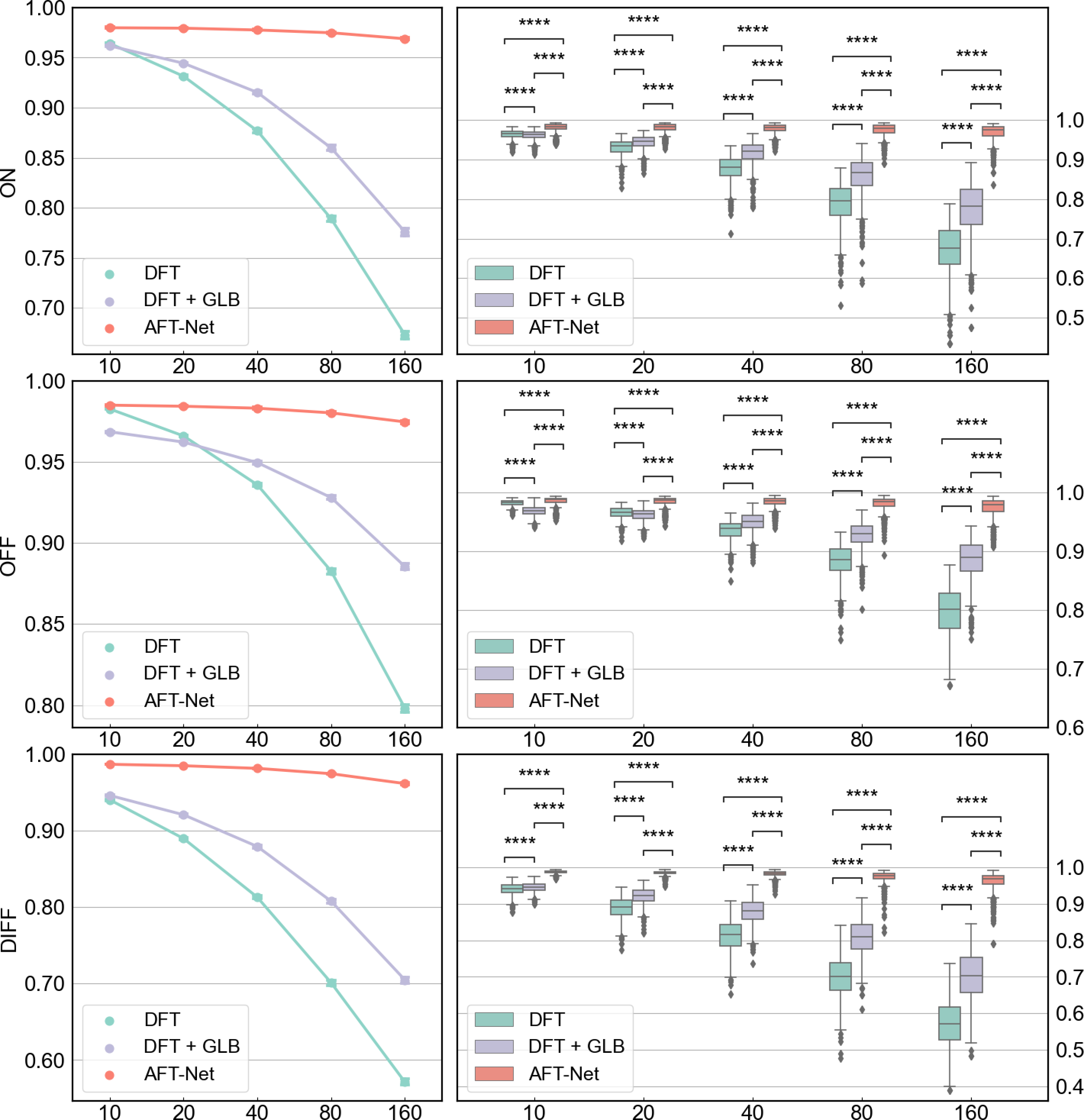
Figure 13: Results of human 3T MRS denoised reconstruction by comparing AFT-Net (I Model), DFT, and DFT with Gaussian line broadening in terms of GFC. p-values indicate results from two-sided t-tests for paired samples. (ns: $p>0.05$, *: $p\leq 0.05$, **: $p\leq 0.01$, ***: $p\leq 0.001$, ****: $p\leq 0.0001$)

Magnetic resonance spectroscopy, namely MRS, is widely used for measuring human metabolism. While MRS has the potential to be highly valuable in clinical practice, it poses several challenges such as low signal-to-noise ratio, overlapping metabolite signals, experimental artifacts, and long acquisition times. Here, the AFT-Net is leveraged as a unified MRS reconstruction approach, which aims to reconstruct and process the FID in parallel, as shown in Figure 12.

We trained our model on the MEGA-PRESS spectra from the Big GABA dataset for two reasons. First, as a proof of concept study, to guarantee the convergence of the supervised learning task, we need the dataset to be sufficient in the number of samples, good in data quality, and publicly available. Thus the Big GABA dataset perfectly meets our requirements. Second, the smaller targeted signals are revealed by the subtraction of 2 spectra containing strong signals (OFF and ON), which provide a good way to verify the performance of the proposed method by measuring the subtraction artifacts. A total number of 101 subjects acquired by the Philips scanners were used in the training. For each subject, a standard GABA ON/OFF edited MRS acquisition was run, where ON editing pulses were placed at 1.9 ppm and OFF editing pulses were placed at 7.46 ppm. The acquisition number is 320 (160 ON and 160 OFF transients) per subject. The AFT-Net was trained with an input size of 2048. The ground truth of the ON/OFF spectra is derived by taking the average over 160 acquisitions. We denote the ground truth as noiseless signals. For the training, we combined randomly sampled acquisitions of each subject to retrieve a noisy signal. By decreasing/increasing the number of sampled acquisitions, we can generate signals with higher/lower noise. We use the reduction rate (R) to denote the level of noise, which is defined as the ratio of the total acquisition number and the number of acquisitions sampled. This quantity is very handy to assess the power of denoising methods in practical terms. Retrieving accurate denoised signals at a high R has implications for the potential reduction of total experimental time.

The results of the AFT-Net approach and conventional numerical methods with Gaussian line broadening are illustrated in Figure 13. The first row shows the reconstructed spectrum from the numerical methods and the proposed AFT-Net. The second row indicates the reconstructed spectrum overlaid with the ground truth. The third row plots the difference between the reconstructed spectrum and the ground truth. Under a reduction rate of 80, where only 2 acquisitions were used over all 160 acquisitions, the AFT-Net shows excellent performance at high reduction rates. The AFT-Net outperforms other methods for the DIFF spectra, indicating that the AFT-Net removes the noise in the FIDs while preserving the subject-level features. We used the Goodness-of-Fit Coefficient (GFC) to measure the similarity between the reconstructed spectra and the ground truth, as shown in the Table 4. The metric value increases as the reduction rate decreases, but the absolute difference between high and low reduction rates is tiny (0.9798 for OFF spectra under a reduction rate of 10 vs. 0.9688 for OFF spectra under a reduction rate of 160). In addition, AFT-Net outperforms the DFT+GLB (Gaussian Line Broadening) method across all metrics in the table.

R	Spectrum	DFT	DFT+GLB	AFT-Net
10	ON	0.9827 ± 0.0047	0.9686 ± 0.0086	0.9850 ± 0.0085
	OFF	0.9641 ± 0.0104	0.9617 ± 0.0108	0.9798 ± 0.0124
	DIFF	0.9403 ± 0.0164	0.9461 ± 0.0126	0.9868 ± 0.0037
20	ON	0.9660 ± 0.0090	0.9622 ± 0.0111	0.9843 ± 0.0092
	OFF	0.9314 ± 0.0192	0.9443 ± 0.0170	0.9794 ± 0.0127
	DIFF	0.8897 ± 0.0283	0.9208 ± 0.0206	0.9849 ± 0.0055
40	ON	0.9359 ± 0.0162	0.9496 ± 0.0155	0.9831 ± 0.0098
	OFF	0.8768 ± 0.0318	0.9152 ± 0.0281	0.9776 ± 0.0139
	DIFF	0.8129 ± 0.0418	0.8792 ± 0.0325	0.9815 ± 0.0078
80	ON	0.8826 ± 0.0280	0.9280 ± 0.0214	0.9803 ± 0.0120
	OFF	0.7890 ± 0.0486	0.8598 ± 0.0452	0.9748 ± 0.0160
	DIFF	0.7010 ± 0.0566	0.8077 ± 0.0480	0.9745 ± 0.0154
160	ON	0.7981 ± 0.0403	0.8854 ± 0.0325	0.9747 ± 0.0160
	OFF	0.6730 ± 0.0619	0.7759 ± 0.0638	0.9688 ± 0.0200
	DIFF	0.5710 ± 0.0654	0.7047 ± 0.0662	0.9616 ± 0.0245

Table 4: GFC metric of human 3T MRS denoised reconstruction. Numbers are presented as mean value ± standard deviation. Numbers in boldface indicate the best metric out of all the methods.

5 Discussion

In this study, a unified MR image reconstruction framework is proposed, which is composed of two main components: artificial Fourier transform block and complex-valued residual attention U-Net. The AFT block is used to approximate the conventional DFT, which is demonstrated in LABEL:tab:fastMRI_recon and LABEL:tab:M4Raw_recon and proofed in Section 3.1. The front-end/back-end convolutional layers are used to extract higher features in the k-space/image domains and play different roles in various tasks. As shown in LABEL:tab:fastMRI_acc_recon, LABEL:tab:M4Raw_acc_recon and 2, both front-end and back-end convolutional layers show superior accelerated reconstruction performance under all sampling ratios compared with single front-end/back-end convolutional layers. This is potentially because the undersampling is performed in k-space where the artifacts are separated from the non-artifact. While in the image domain, it is converted to aliasing overlapped over the whole image. The artifacts removal task can be recast as an image inpainting problem in the k-space domain which can be done more easily by the front-end convolutional layers. The superiority of front-end convolutional layers does not always hold for all tasks, as can be seen in LABEL:tab:fastMRI_denoise_recon, LABEL:tab:M4Raw_denoise_recon and 3, where back-end only convolutional layers outperform the front-end and back-end convolutional layers on the denoised reconstruction task. Although the linearity of the Fourier transform and the property that the Fourier transform of Gaussian noise is still Gaussian noise guarantee the possible workaround of denoising in both k-space and image domain, the sparse representation of k-space data makes it harder for a convolutional network to extract noise information in the low-frequency areas. Therefore, all the structures with front-end convolutional layers show lower performance, indicating that k-space noise removal with a convolutional network may not be a preferable approach.

Domain-transform manifold learning has been introduced for years and several deep learning frameworks were developed based on this idea. The first model, AUTOMAP [14], proposed the simple FC-Conv structure which can only be applied to images with small matrix size due to its redundant FC layers. DOTA-MRI [16] extended AUTOMAP to Conv-FC-Conv structure and applied FC layers to only one dimension (phase-encoding direction). However, it only applied to 1D undersampling and did not work on 2D undersampling (e.g. 2D Gaussian random sampling or 2D Poisson sampling). The AFT-Net we proposed in this study solves the problem mentioned above through a modular-designed AFT block. We also demonstrated that the extended AFT-Net can also be applied to 1D data in Section 4.2.4. In addition, previous works define the loss in the magnitude image, while we calculate the loss in the complex-valued image domain, which preserves the relations between the real and imaginary parts. The phase is then derived from the output of AFT-Net, which is essential for several phase-based applications, such as flow quantification and fat–water separation.

Complex-valued neural networks, especially complex-valued convolutional networks [24, 23], have been studied for MRI reconstruction but they mainly focused on simple tasks or only applied it to the image domain. We investigate the different impacts of complex-valued convolutional networks on the k-space and image domain and extend the application to accelerated reconstruction and denoised reconstruction, which are more clinically important. We also incorporate domain-manifold learning by adding domain transform blocks which determine the mapping between the k-space and image domain instead of conventional discrete Fourier transform. It is more robust to noise and signal nonideality due to imperfect acquisition. We also extend the application of complex-valued convolutional networks to 1D MRS denoised reconstruction, which has not been studied in previous work.

One remaining methodological limitation is that the FC layers used by AFT-Net narrow the application to datasets with various image matrix sizes. Although the convolutional layers are not sensitive to the image matrix sizes and cropping/padding can be applied to match the desired sizes, the features of FC layers need to be selected carefully which requires further investigation. Another parameter that needs to be taken into account is the coil number. In this study, we selected especially 4-channel MRI data for convenience of data preprocessing. While deep learning-based coil combinations could be incorporated into the framework in future work. Furthermore, diffusion models are shown to be a powerful tool for image reconstruction across body regions and coil numbers [17]. However, the score-MRI we compared in this study does not demonstrate superior performance compared with AFT-Net and the inference stage time is extremely long. This is potentially because the backbone of the score-MRI is still a real-valued U-Net like structure and the relation between the real and imaginary part is not considered during the calculation of the score function. For future works, the AFT-Net could be further extended by leveraging diffusion-based models with complex-valued convolutional networks as the backbone and careful optimization to reduce the inference time.

6 Conclusion

In conclusion, we propose AFT, a novel artificial Fourier transform framework that determines the mapping between k-space and image domain as conventional DFT while having the ability to be fine-tuned/optimized with further training. The flexibility of AFT allows it to be easily incorporated into any existing deep learning network as learnable or static blocks. We then utilized AFT to design our AFT-Net, which implements complex-valued U-Net to extract higher features in the k-space and/or image domain. We aim to combine reconstruction and acceleration/denoising tasks into a unified network that simultaneously enhances the image quality by removing artifacts directly from the k-space and/or image domain. The proposed methods are evaluated on datasets with additional artifacts, different contrasts, and different modalities. Our AFT-Net achieves competitive results compared with other methods and proves to be more robust to noise and contrast differences. An extensive study on various system fields, various species, various modalities, various input dimensions, and various tasks demonstrates the effectiveness and generality of AFT-Net.

References

- [1] J. Zbontar, F. Knoll, A. Sriram, T. Murrell, Z. Huang, M. J. Muckley, A. Defazio, R. Stern, P. Johnson, M. Bruno, et al., “fastmri: An open dataset and benchmarks for accelerated mri,” arXiv preprint arXiv:1811.08839, 2018.
- [2] M. Lyu, L. Mei, S. Huang, S. Liu, Y. Li, K. Yang, Y. Liu, Y. Dong, L. Dong, and E. X. Wu, “M4raw: A multi-contrast, multi-repetition, multi-channel mri k-space dataset for low-field mri research,” Scientific Data, vol. 10, no. 1, p. 264, 2023.
- [3] M. Mikkelsen, P. B. Barker, P. K. Bhattacharyya, M. K. Brix, P. F. Buur, K. M. Cecil, K. L. Chan, D. Y.-T. Chen, A. R. Craven, K. Cuypers, et al., “Big gaba: Edited mr spectroscopy at 24 research sites,” Neuroimage, vol. 159, pp. 32–45, 2017.
- [4] G. Georgiou and C. Koutsougeras, “Complex domain backpropagation,” IEEE Transactions on Circuits and Systems II: Analog and Digital Signal Processing, vol. 39, no. 5, pp. 330–334, 1992.
- [5] N. Guberman, “On complex valued convolutional neural networks,” arXiv preprint arXiv:1602.09046, 2016.
- [6] C. Trabelsi, O. Bilaniuk, Y. Zhang, D. Serdyuk, S. Subramanian, J. F. Santos, S. Mehri, N. Rostamzadeh, Y. Bengio, and C. J. Pal, “Deep complex networks,” in International Conference on Learning Representations, 2018.
- [7] J. B. Johnson, “Thermal agitation of electricity in conductors,” Physical review, vol. 32, no. 1, p. 97, 1928.
- [8] H. Nyquist, “Thermal agitation of electric charge in conductors,” Physical review, vol. 32, no. 1, p. 110, 1928.
- [9] M. S. Hansen and P. Kellman, “Image reconstruction: an overview for clinicians,” Journal of Magnetic Resonance Imaging, vol. 41, no. 3, pp. 573–585, 2015.
- [10] J. A. Fessler, “Model-based image reconstruction for mri,” IEEE signal processing magazine, vol. 27, no. 4, pp. 81–89, 2010.
- [11] M. De Bruijne, “Machine learning approaches in medical image analysis: From detection to diagnosis,” 2016.
- [12] J. W. Cooley and J. W. Tukey, “An algorithm for the machine calculation of complex fourier series,” Mathematics of computation, vol. 19, no. 90, pp. 297–301, 1965.
- [13] D. Shen, G. Wu, and H.-I. Suk, “Deep learning in medical image analysis,” Annual review of biomedical engineering, vol. 19, pp. 221–248, 2017.
- [14] B. Zhu, J. Z. Liu, S. F. Cauley, B. R. Rosen, and M. S. Rosen, “Image reconstruction by domain-transform manifold learning,” Nature, vol. 555, no. 7697, pp. 487–492, 2018.
- [15] J. López-Randulfe, T. Duswald, Z. Bing, and A. Knoll, “Spiking neural network for fourier transform and object detection for automotive radar,” Frontiers in Neurorobotics, vol. 15, p. 688344, 2021.
- [16] T. Eo, H. Shin, Y. Jun, T. Kim, and D. Hwang, “Accelerating cartesian mri by domain-transform manifold learning in phase-encoding direction,” Medical Image Analysis, vol. 63, p. 101689, 2020.
- [17] H. Chung and J. C. Ye, “Score-based diffusion models for accelerated mri,” Medical image analysis, vol. 80, p. 102479, 2022.
- [18] K. Xu, M. Qin, F. Sun, Y. Wang, Y.-K. Chen, and F. Ren, “Learning in the frequency domain,” in Proceedings of the IEEE/CVF conference on computer vision and pattern recognition, pp. 1740–1749, 2020.
- [19] A. Hirose, Complex-valued neural networks, vol. 400. Springer Science & Business Media, 2012.
- [20] A. Hirose and S. Yoshida, “Generalization characteristics of complex-valued feedforward neural networks in relation to signal coherence,” IEEE Transactions on Neural Networks and learning systems, vol. 23, no. 4, pp. 541–551, 2012.
- [21] M. Tygert, J. Bruna, S. Chintala, Y. LeCun, S. Piantino, and A. Szlam, “A mathematical motivation for complex-valued convolutional networks,” Neural computation, vol. 28, no. 5, pp. 815–825, 2016.
- [22] O. Ronneberger, P. Fischer, and T. Brox, “U-net: Convolutional networks for biomedical image segmentation,” in Medical Image Computing and Computer-Assisted Intervention–MICCAI 2015: 18th International Conference, Munich, Germany, October 5-9, 2015, Proceedings, Part III 18, pp. 234–241, Springer, 2015.
- [23] D. Sikka, N. Igra, S. Gjerwold-Sellec, C. Gao, E. Wu, and J. Guo, “Cu-net: A completely complex u-net for mr k-space signal processing,” in ISMRM (International Society of Magnetic Resonance Imaging) Virtual Conference & Exhibition, 2021, Internationala Society of Magnetic Resonance Imaging (ISMRM)., 2021.
- [24] E. Cole, J. Cheng, J. Pauly, and S. Vasanawala, “Analysis of deep complex-valued convolutional neural networks for mri reconstruction and phase-focused applications,” Magnetic resonance in medicine, vol. 86, no. 2, pp. 1093–1109, 2021.
- [25] S. Ioffe and C. Szegedy, “Batch normalization: Accelerating deep network training by reducing internal covariate shift,” in International conference on machine learning, pp. 448–456, pmlr, 2015.
- [26] Y. Wu and K. He, “Group normalization,” in Proceedings of the European conference on computer vision (ECCV), pp. 3–19, 2018.
- [27] J. L. Ba, J. R. Kiros, and G. E. Hinton, “Layer normalization,” arXiv preprint arXiv:1607.06450, 2016.
- [28] D. P. Kingma and J. Ba, “Adam: A method for stochastic optimization,” arXiv preprint arXiv:1412.6980, 2014.
- [29] P. B. Roemer, W. A. Edelstein, C. E. Hayes, S. P. Souza, and O. M. Mueller, “The nmr phased array,” Magnetic resonance in medicine, vol. 16, no. 2, pp. 192–225, 1990.
- [30] A. Deshmane, V. Gulani, M. A. Griswold, and N. Seiberlich, “Parallel mr imaging,” Journal of Magnetic Resonance Imaging, vol. 36, no. 1, pp. 55–72, 2012.
- [31] Z. Wang, E. P. Simoncelli, and A. C. Bovik, “Multiscale structural similarity for image quality assessment,” in The Thrity-Seventh Asilomar Conference on Signals, Systems & Computers, 2003, vol. 2, pp. 1398–1402, Ieee, 2003.
- [32] J. Romero, A. Garcıa-Beltrán, and J. Hernández-Andrés, “Linear bases for representation of natural and artificial illuminants,” JOSA A, vol. 14, no. 5, pp. 1007–1014, 1997.