Low-latency Space-time Supersampling for Real-time Rendering

Abstract

With the rise of real-time rendering and the evolution of display devices, there is a growing demand for post-processing methods that offer high-resolution content in a high frame rate. Existing techniques often suffer from quality and latency issues due to the disjointed treatment of frame supersampling and extrapolation. In this paper, we recognize the shared context and mechanisms between frame supersampling and extrapolation, and present a novel framework, Space-time Supersampling (STSS). By integrating them into a unified framework, STSS can improve the overall quality with lower latency. To implement an efficient architecture, we treat the aliasing and warping holes unified as reshading regions and put forth two key components to compensate the regions, namely Random Reshading Masking (RRM) and Efficient Reshading Module (ERM). Extensive experiments demonstrate that our approach achieves superior visual fidelity compared to state-of-the-art (SOTA) methods. Notably, the performance is achieved within only 4ms, saving up to 75% of time against the conventional two-stage pipeline that necessitates 17ms.

Introduction

Recently, the rendered contents have been a spotlight in Human-Computer Interaction (HCI) applications, spanning personal computers, mobile devices, and VR/AR hardware. Notably, the Meta Quest 2 VR headset supports an impressive 90 Hz frame rate with 1832x1920 resolution per eye. Meanwhile, Unreal Engine 5 can create photorealistic 3D environments using real-time ray tracing and physically-based shading. However, these advances pose a significant challenge for the limited hardware. Low resolution (LR) and low frame rate (LFR) significantly affect the user’s immersion, as users are sensitive to both the details and the smoothness of rendered frames, which lies over 90Hz (Shi et al. 2023). The post-processing methods provide a plausible solution to increase resolution and frame rate.

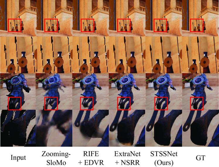
Figure 1: Visual comparison with the state-of-the-arts. The input has the aliasing caused by low-resolution rendering (Up) and the warping hole by frame extrapolation (Down). Our method can address them well in a unified pipeline.

Neural networks have demonstrated remarkable performance in enhancing video resolution and frame rate before their application to rendered content. Existing literature has explored video super-resolution (Liang et al. 2022; Li et al. 2023), frame interpolation (Huang et al. 2022; Plack et al. 2023) and space-time video super-resolution (Geng et al. 2022; Hu et al. 2023). Nonetheless, simply transferring these video processing methods to real-time rendering reveals two evident shortcomings, as shown in Fig. 2(a): (1) Not effective in addressing aliasing. The aliasing in rendered content is caused by a low point sampling rate, while the pixels in photographic images are formed by integrating light rays. The fragmented object, such as the spear, can not be adequately compensated using conventional video methods. (2) High processing latency. The video methods primarily emphasize interpolation over extrapolation, which implies that the future frame ($T+1$) is needed first before generating the current frame ($T$). The methods unavoidably introduce extra display delay and spoil the user experience. Consequently, addressing these major drawbacks requires more effective methodologies tailored for real-time rendering.

Existing rendering techniques (Akeley 1993; Lottes 2009; Karis 2014) enhance rendering quality by leveraging G-buffers and the motion vectors (MV). In real-time rendering, the engine first generates the G-buffers by fast preprocessing passes before the time-consuming frame rendering, as illustrated in Fig. 2(b). G-buffer contains the intrinsic details about objects before shading with light. We can generate base color, roughness, metallic, world normal, world position, scene depth, and many other results, covering from material to position. Also, the motion vectors (MV) can be calculated analytically from the 3D point displacements ahead of the rendering. MV facilitates warping and aligning the frames, akin to the role of optical flow in video processing. Consequently, G-buffer and motion vector provide practical information for post-processing.

Recent state-of-the-art methods employ neural networks for learned rendering post-processing. Frame supersampling (Xiao et al. 2020) and frame extrapolation (Guo et al. 2021) approaches are proposed to address the LR and LFR problems separately, as depicted in Fig. 2(b1). Though frame extrapolation has low latency, it introduces warping holes because of the occlusion. Meanwhile, supersampling methods still have problems with the aliasing. Previous methods fall short in terms of performance and efficiency without considering the shared context and mechanism in solving the aliasing and warping holes, as in Fig. 1.

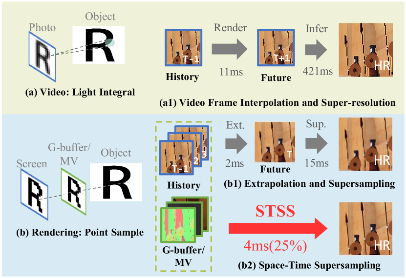
Figure 2: Comparison of different architectures in video and rendered content processing. We show the inference time targeting 1080P. Our framework can achieve better quality at a much faster inferencing speed.

Overall, the rendering post-processing calls for a unified approach to address the low resolution and low frame rate problem. Inspired by recent advancements in space-time video super-resolution(STVSR) works (Xiang et al. 2020), we introduce the concept of the space-time supersampling (STSS) problem. Specifically, a frame should be supersampled if it is rendered by the engine and, conversely, should be generated from previous frames if not rendered. Different from STVSR, STSS utilizes the G-buffer and MV provided by the rendering engines to meet the demand for higher resolution and frame rate (usually 1080P at 60Hz). Our contribution to the problem can be summarized as:

1. To our best knowledge, we propose the first unified space-time supersampling (STSS) framework for real-time rendering, exploiting the common context and mechanism of frame extrapolation and supersampling. Our method achieves state-of-the-art performance among STSS pipelines.

2. Our framework streamlines the workflow by adopting a unified context and a shared neural network. It only requires 4ms per frame at 1080P settings, compared to 17ms by previous methods, saving up to 75% time.

3. We introduce a novel reshading mechanism that uniformly addresses the aliasing and warping holes as reshading regions. To achieve better reshading performance, we propose the Reshading Random Masking (RRM) and Efficient Reshading Module (ERM).

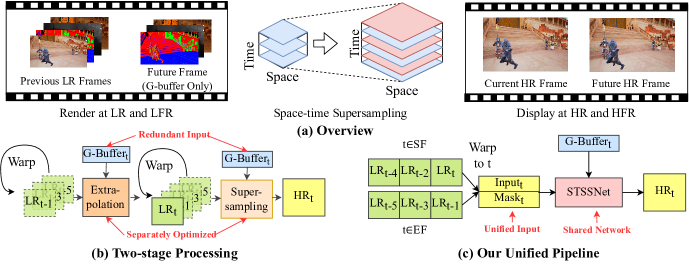
Figure 3: Overview of the space-time supersampling (STSS) pipeline. The pipeline generates the supersampled frame and the future frame, and users get HR results with a double frame rate. Previous works (b) separately execute frame extrapolation and supersampling with redundancy, while we exploit the common context and mechanism to build a unified pipeline (c).

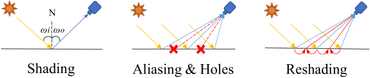
Figure 4: Illustration of shading and reshading mechanism. Aliasing and holes are not shaded in LR and LFR rendering.

Related Work

Spatial and Temporal Supersampling

The rendering content suffers aliasing because the content is undersampled in low resolution. One straightforward solution is supersampling antialiasing (SSAA), which downsamples the target frame rendered in a larger resolution. It will effectively reduce the aliasing but at a very high cost. Then, MSAA (Akeley 1993), MLAA (Reshetov 2009), FXAA (Lottes 2009) are proposed to improve the efficiency. Nevertheless, the spatial antialiasing methods ignore temporal coherence and may produce artifacts in large motion. TAA (Karis 2014) is a widely-adopted algorithm that uses history frames to suppress flicker. TAAU (EpicGames 2020) and FSR (GPUOpen-Effects 2022) can further upsample the results while preserving consistency.

Recently, neural networks have been applied to real-time rendering. For supersampling, (Xiao et al. 2020; Thomas et al. 2020; Guo et al. 2022) exploit the temporal feature to upscale the low-resolution frames and (Thomas et al. 2022; Li et al. 2022) can also handle noisy LR renderings. For frame generation, (Briedis et al. 2021, 2023) interpolates the offline rendered content, and (Guo et al. 2021) is the first to extrapolate the future frame for a lower latency. There are also device-specific post-processing products for neural supersampling, such as DLSS (Andrew Edelsten and Patney 2019) and XeSS (Chowdhury et al. 2022). DLSS3 (Lin and Burnes 2022) further introduces a separate network for frame generation. Since most codes are unavailable, we compare with two open-sourced baselines via training, NSRR (Xiao et al. 2020) and ExtraNet (Guo et al. 2021), and compare other methods through provided software. Unlike previous works, our model has unified supersampling and extrapolation to achieve better quality and lower latency.

Video Super-resolution and Frame Interpolation

Video super-resolution (VSR) (Wang et al. 2019; Liang et al. 2022; Li et al. 2023) aims to increase the spatial resolution of the video. In contrast, video frame interpolation (VFI) (Ding et al. 2021; Huang et al. 2022; Plack et al. 2023) increases the temporal resolution, i.e., predicting the unknown frame between existing frames. Other than addressing the problems separately, the space-time video super-resolution (STVSR) (Xiang et al. 2020; Geng et al. 2022; Hu et al. 2023) aims to expand the space and time resolution simultaneously, which is joint processing of VSR and VFI. We also notice existing video prediction and extrapolation methods (Oprea et al. 2020; Wu, Wen, and Chen 2022). However, the video methods fail to consider the rendering intrinsic mechanism, leading to the aliasing problem and significant latency.

Methodology

Unified Space-time Supersampling Framework

The low-resolution and low-frame-rate problems are pivotal concerns in real-time rendering and lead to poor user experience. Fig. 3(a) illustrates the ideal prospect of rendering at LR and LFR and displaying at HR and HFR. Existing post-processing techniques have been proposed to address these issues individually. NSRR (Xiao et al. 2020) utilizes convolutional neural networks for spatial supersampling, while ExtraNet (Guo et al. 2021) extrapolates future frames to achieve reduced display latency.

An intuitive approach involves integrating current supersampling and extrapolation methods into a two-stage pipeline, as depicted in Figure 3(b). However, this approach introduces significant redundancy in context and mechanism. The frame extrapolation and supersampling are executed independently with similar input of the previous frames and the G-buffer of the current frame. Then, both methods employ motion vectors to warp historical frames and leverage G-buffer for frame reconstruction. The only difference is the time step of input data. Consequently, the pipeline results in notable latency and poor performance.

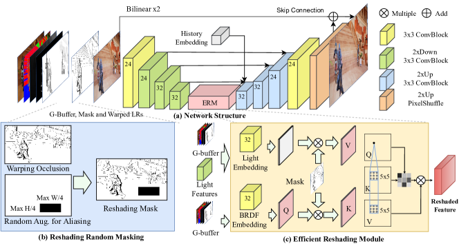
Figure 5: Network architecture of our unified space-time supersampling framework with RRM(b) and ERM(c). The numbers on the block denote the output channels of the convolution layer.

In this paper, we first formulate our space-time supersampling(STSS) framework, as shown in Fig. 3(c). Given the different time step $t$, the output $HR_{t}$ can be expressed as:

$$HR_{t}=\left\{\begin{matrix}\Phi(LR_{t-5,t-3,t-1},G_{t},MV_{t-5,...,t}),&t\in EF\\ \Phi(LR_{t-4,t-2,t},G_{t},MV_{t-4,...,t}),&t\in SF\end{matrix}\right.$$ (1)

where $\Phi$ is the shared network for STSS. $G_{t}$ and $MV_{t}$ stand for G-buffer and MV at frame $t$. We denote the rendered frames as Supersampling Frames(SF) and the others as Extrapolation Frames (EF). We use three successive frames for SF, noted as $LR_{t}$, $LR_{t-2}$, and $LR_{t-4}$. Their G-buffer and MV are generated from $t$ to $t-4$ for every frame. The LR frames are all warped to $LR_{t}$ using the MV and producing warping masks. The warped LR frames, their warping mask, and the G-buffer are provided to the model to predict $HR_{t}$. On the other hand, we use $LR_{t-1}$ to $LR_{t-5}$ for EF. They are all warped to the future frame $LR_{t}$ using the motion vector from $t$ to $t-5$. STSS aims to minimize the perceptual difference between the generated and ground truth HR frames. So far, we unify the form to reduce the context redundancy.

Reshading Mechanism

The primary challenges of STSS comprise the aliasing resulting from low-resolution sampling and the warping holes due to frame extrapolation. Here, we dig deeper into the rendering principles for reducing the mechanism redundancy of addressing these two regions. The render engine performs shading (to calculate colors for every pixel) using the following equation(Kajiya 1986):

$$L_{o}(p,\omega_{o})=\int_{\Omega^{+}}L_{i}(p,\omega_{i})f_{r}(p,\omega_{i},\omega_{o})\cos\theta_{i}\mathrm{d}\omega_{i}$$ (2)

where, $L_{o}(p,\omega_{o})$ is the outgoing light at a shading point $p$ with direction $\omega_{o}$. $L_{i}$ is the incoming light from all possible directions, $\Omega^{+}$ and $\theta_{i}$ is the angle to the normal vector. $f_{r}(p,\omega_{i},\omega_{o})$ is the bidirectional reflectance distribution function (BRDF) describing the relation of incoming and outgoing radiance. BRDF and relative positions can be described with the G-buffer. We observe that a shared, significant characteristic between the aliasing regions and the warping holes is the absence of correct shading due to low rendering sampling rate in space and time.

As shown in Fig. 4, we propose reshading mechanism (to re-calculate colors from shaded pixels) to treat these two regions unified as the reshading regions. The reshading mechanism involves a similar process as shading, which uses the BRDF and the light to calculate the reshaded feature, and an aggregation of adjacent regions. Specifically, we propose to replace the BRDF and the light in Eqa. 2 with G-buffer and predicted light features. Then, we reshade the color in the feature space, formulated as follows:

$$\phi(p)=\int_{\Omega_{p}}(L(p+\delta)*G(p+\delta))R(p,p+\delta)\mathrm{d}\delta$$ (3)

where $\phi(p)$ is the reshaded feature for the point $p$. $L$ is the light feature extracted from inputs, $G$ is the G-buffer and $*$ is a reshading function. We aggregate the reshaded feature in the adjacent region $\Omega_{p}$. $R(p,p+\delta)$ describes the similarity of $p$ and $p+\delta$, which serves as a normalization weight. Since the local shading depends on the BRDF and the visibility, we can infer $R(p,p+\delta)$ from the G-buffer and the mask. The reshading unifies the mechanism in the STSS problem and shows a feasible and efficient design.

Network Architecture

Fig. 5(a) shows the structure of our proposed STSSNet. We adopt a U-Net (Ronneberger, Fischer, and Brox 2015) structure as our backbone. Our network takes as input the warped LRs (including $LR_{t-5,t-3,t-1}$), the G-buffer and the masks. The G-buffer includes base color, normal, depth, metallic, and roughness, which describes the BRDF and position in pixels. The input is first augmented with Reshading Random Masking (RRM). The mask is applied to the input and concatenated with the original one to feed into the network. Subsequently, we extract the features by several convolutional layers, followed by the Efficient Reshading Module (ERM). To capture temporal context, we utilize the history embedding(Guo et al. 2021), which encodes the previous frames and their warping mask. Then the features are fused with the history embedding and upsampled to get the final output.

Random Reshading Masking.

To handle both the warping holes and the aliasing regions, we propose the concept of Random Reshading Masking (RRM), as depicted in Fig. 5(b). Though previous applications of random masking have been observed in tasks like classification (Zhong et al. 2020) and optical flow estimation (Teed and Deng 2020), RRM has a distinctive function.

According to Eqa. 3, the mask affects how the reshading mechanism aggregates from adjacent regions. But the input mask is limited to warping holes. Therefore, we use random augmentation to bring aliasing regions into the mask and make the model more robust. Concretely, we add randomly sized rectangles smaller than 1/4 of the frame’s width and height at random positions to the occlusion mask. Then, we concatenate the modified LR images and G-buffers with the unaltered ones across channels for the network input. Also, we punish the masked areas with a larger loss.

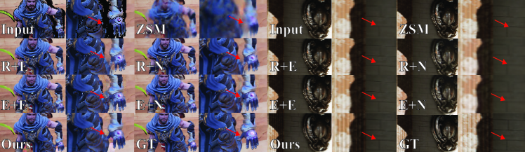
Figure 6: Qualitative comparison with SOTA methods. From left to right and up to down: Input, Zooming-SloMo, RIFE+EDVR, RIFE+NSRR, ExtraNet+EDVR, ExtraNet+NSRR, Ours, GT. The black regions are the warping holes and the red arrows are indicating the interested regions. Please zoom in for better view.

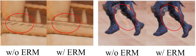
Figure 7: Effect of ERM. The module can recover the details in both the aliasing regions and warping holes.

Efficient Reshading Module.

Fig. 5(c) shows the structure of ERM. While the backbone has partially addressed reshading problems through convolution layers, the awareness of G-buffer is lacking and the problems of the aliasing and warping holes still exist. To address the problems, our module incorporates a local attention mechanism to fuse features from nearby regions of the similar G-buffer.

Initially, we concatenate the downsampled G-buffer with the light features from the backbone, encoding them as the Light Embedding. Meanwhile, the G-buffer is encoded into the BRDF Embedding. Then, we take the BRDF Embedding as Q map and multiply the Mask to the BRDF/Light Embedding as K/V map for attention. $\textbf{Q}(p)$ is the attention query for every point $p$, including warping holes. We mask the value in the warping holes as zero, and get $\textbf{K}(p+\delta)$, which is the attention key for points $p+\delta$ in the local window $\Omega_{p}$ of the $p$:

$$\textbf{K}(p+\delta)=\left\{\begin{array}[]{ll}\textbf{Q}(p+\delta)&\text{ if }\mathbf{ValidMask}(p+\delta)=1\\ 0&\text{ otherwise }\end{array}\right..$$ (4)

It means that $\textbf{Q}(p)\textbf{K}^{T}(p+\delta)$ of warping holes $p+\delta$ in the local window is zero. Therefore, $\textbf{V}(p+\delta)$ of the warping holes (including the query point $p$ itself) will be ignored, and the only features from nearby valid regions are fused.

Finally, the attention computation employs linear units (Zhang, Titov, and Sennrich 2021) within a sliding window:

$$\phi(p)=\sum_{\Omega_{p}}\operatorname{Relu}(\textbf{Q}(p)\textbf{K}^{T}(p+\delta))\textbf{V}(p+\delta)$$ (5)

where the attention is calculated only in the local $5\times 5$ window $\Omega_{p}$ of each shading point $p$, so ERM has a small amount of computation (only 10% of the backbone). Fig. 7 shows that ERM gathers light embeddings from adjacent regions with similar BRDF and recovers the details.

	Scene	RIFE+EDVR	RIFE+NSRR	ExtraNet+EDVR	ExtraNet+NSRR	ZoomingSloMo	STSSNet(Ours)
PSNR$\uparrow$	LE	30.38/29.57	34.28/32.28	30.45/30.29	34.29/33.87	30.39/28.51	35.02/34.72
	ST	30.97/28.46	31.41/28.7	31.03/30.02	31.45/30.24	31.00/27.35	32.18/30.25
	SW	28.32/26.05	29.93/27.01	28.71/28.32	30.18/29.88	28.17/24.79	31.00/30.35
	AR*	31.52/28.95	33.26/29.59	31.52/31.42	33.14/31.97	31.36/25.86	33.36/32.40
SSIM$\uparrow$	LE	0.912/0.891	0.953/0.927	0.910/0.910	0.953/0.951	0.913/0.891	0.957/0.956
	ST	0.918/0.862	0.921/0.864	0.920/0.909	0.923/0.911	0.920/0.851	0.926/0.913
	SW	0.876/0.795	0.892/0.814	0.880/0.877	0.899/0.892	0.874/0.780	0.908/0.899
	AR*	0.940/0.889	0.942/0.886	0.932/0.937	0.940/0.923	0.937/0.809	0.943/0.934
LPIPS$\downarrow$	LE	0.135/0.131	0.090/0.097	0.132/0.135	0.080/0.089	0.050/0.054	0.018/0.020
	ST	0.138/0.165	0.149/0.188	0.136/0.159	0.148/0.179	0.059/0.091	0.048/0.059
	SW	0.195/0.201	0.213/0.250	0.185/0.195	0.185/0.204	0.188/0.267	0.140/0.162
	AR*	0.097/0.102	0.107/0.134	0.100/0.100	0.111/0.144	0.037/0.055	0.021/0.027
VMAF$\uparrow$	LE	56.33	69.66	59.38	73.41	59.25	78.85
	ST	60.98	64.30	68.17	71.60	58.80	75.71
	SW	54.79	64.47	64.48	76.87	49.98	81.16
	AR*	72.60	78.84	80.37	86.05	63.59	85.15

Table 1: Quantitative comparison on PSNR, SSIM, LPIPS, VMAF. We show the indicators separately for the supersampling frames (SF)/ the extrapolated frames (EF). Lewis (LE), SunTemple (ST), Subway (SW), and Arena (AR) are the names of different scenes. The evaluation on AR (marked with *) follows the cross-scene setting. Bold text indicates the best results.

Loss Function.

Our loss function can be separated into two parts: weighted L1 loss and perceptual loss. First, we use the L1 loss to constrain the photometric consistency and punish the reshading regions for a larger weight. Our weighted L1 loss can be described as follows.

$$L_{l1}(I,\hat{I})=\frac{1}{mn}\sum_{i=1}^{m}\sum_{j=1}^{n}w_{i,j}|I_{i,j}-\hat{I}_{i,j}|$$ (6)

where $(i,j)$ represents the point in the output $\hat{I}$ and the ground truth $I$. $m,n$ represents the height and width. $w_{i,j}$ is the loss weight, which is 2 in the reshading mask and 1 for other regions. Second, we add a perceptual loss (Zhang et al. 2018) to improve perceptual fidelity. This work adopts a pre-trained VGG (Simonyan and Zisserman 2014) network and calculates the per-layer similarity as the metric. Finally, our total loss function can be represented as $L(I,\hat{I})=L_{l1}(I,\hat{I})+w_{p}L_{p}(I,\hat{I})$, where $L_{p}$ is the perceptual loss, and $w_{p}$ is the weight. Empirically, we set $w_{i,j}=1$ and $w_{p}=0.01$.

Datasets and Preprocessing

In order to evaluate models for the novel STSS task, we propose a high-quality rendering dataset with LR-LFR and HR-HFR pairs. We combine the dataset construction protocol of the previous supersampling(Xiao et al. 2020) and extrapolation works (Guo et al. 2021). (1) Dataset Generation: We construct scenes and actions, render them using Unreal Engine, and extract the G-buffer and motion vector. We turn on ray tracing and shadows for more realistic effects. It contains four scenes, Lewis(LE), SunTemple(ST), Subway(SW), and Arena(AR), each with 6000 frames for training and 1000 for testing. (2) Resolution Configuration: For LR-LFR frames, we turn off antialiasing and render at $960\times 540$ resolution at 30FPS. For HR-HFR frames, we first render at $3840\times 2160$ resolution at 60FPS and then downsample it to $1920\times 1080$ resolution as a $16\times$ supersampling ground truth. Therefore, supersampling frames (SF) take up 50% of the frames and extrapolation frames (EF) for the other 50%. (3) Preprocessing: The extrapolation motion vectors (Zeng et al. 2021) are used to warp the frames. The motion vector, stencil, world position, normal, and NoV (dot product of the world normal and view vector) in G-buffer are used for generating warping masks following (Guo et al. 2021), while base color, metallic, roughness, depth, and normal for network input.

Models	Edges		Warping Holes
	PSNR $\uparrow$	SSIM $\uparrow$	PSNR $\uparrow$	SSIM $\uparrow$
RIFE+EDVR	17.65	0.524	19.11	0.618
ExtraNet+NSRR	23.36	0.853	25.40	0.849
ZoomingSloMo	18.02	0.543	19.05	0.618
Ours w/o ERM	23.84	0.850	26.44	0.872
Ours	23.95	0.853	26.52	0.874

Table 2: Comparison on different reshading regions.

Models	Time(ms)$\downarrow$		Param(M)$\downarrow$
	Stage1	Stage2	Stage1	Stage2
RIFE+EDVR	19.2	402.2	9.8	20.7
ExtraNet+NSRR	10.3(1.8)	20.4(15.4)	0.3	0.8
ZoomingSloMo	821.1		11.1
STSSNet(Ours)	9.0(4.4)		0.4

Table 3: Comparison of time cost and parameters. The bracket means a reimplementation with TensorRT.

Size	1.LR	2.GB	3.Warp	4.Network	Total	HR
720p	3.56	0.57	0.69	3.86	8.68	19.57
1080p	5.69	0.63	0.81	4.35	11.51	38.38
2160p	19.19	0.97	2.64	17.19	39.99	69.66

Table 4: Time analysis on different resolutions in ms.

Components	Parameters	Computation	Time
Backbone	141.00 K	20.53 GFLOPS	3.39 ms
HistoryEmbedding	120.70 K	8.78 GFLOPS	0.12 ms
ERM	155.54 K	2.20 GFLOPS	0.83 ms
Full	417.24 K	31.50 GFLOPS	4.35 ms

Table 5: Cost analysis for each component.

Experiments

Experimental Settings

We use Pytorch to implement our model. We trained our model for 100 epochs on the training set with the Adam optimizer, and the learning rate was set to 1e-4. The learning rate optimizer is StepLR, with a step size of 50 and a gamma of 0.9. We use RandomCrop for augmentation, and each time we slice the input image into patches of size 256x256, repeat four times and feed them into the network. Following previous work (Guo et al. 2021), we evaluate for single-scene (train and test on LE, ST, and SW) and cross-scene (train on LE, ST, and SW, test on AR) settings.

We compare various SOTA video and rendering methods in two folds. First, for two-stage methods, we combine four baseline models: RIFE (Huang et al. 2022) for VFI, EDVR (Wang et al. 2019) for VSR, NSRR (Xiao et al. 2020) for rendering supersampling, and ExtraNet (Guo et al. 2021) for rendering extrapolation. Next, we also compared the STVSR method ZoomingSloMo (Xiang et al. 2020). We trained the models for 100 epochs in single-scene setting and 50 epochs in cross-scene setting. We then tested them with an RTX 3090 GPU. The latest video methods (Zhou et al. 2021; Geng et al. 2022; Liang et al. 2022) could not be tested because of the large GPU memory footprint over 24G.

Comparison Against the State-of-the-arts

Space-time Supersampling. Tab. 1 shows that our method has a significant advantage on PSNR, SSIM (Wang et al. 2004), LPIPS (Zhang et al. 2018), and most VMAF (Li et al. 2018) indicators. LPIPS is widely used for perceptual image quality assessment, and VMAF is a famous perceptual video quality assessment algorithm developed by Netflix. Moreover, our method has more stable quality for both SFs and EFs, while other methods have a performance drop in EFs. The video processing methods have inferior performance, mainly because of ignoring the G-buffer and MV.

Reshading Regions. Tab. 2 demonstrates the effectiveness of our method on different reshading regions. We compare PSNR and SSIM metrics on the canny edge (thresholds set to 100 and 200) and the warping mask (interpolated from LR input) of EF. Fig. 9 also shows the qualitative comparison in the reshading regions on Lewis dataset. Our method can better handle edges and warping holes than previous methods.

Efficiency Analysis

Inferencing Time Comparison. Our tests run at 540P, targeting 1080P and on RTX 3090 GPU. All models run at half-precision for inference. We follow previous work (Xiao et al. 2020; Guo et al. 2021) to reimplement the rendering models using the TensorRT and show the results in the brackets. Tab. 3 shows that our method only has 0.4M parameters and needs 4.4ms per frame when inferencing, which saves 75% of time for two-stage methods. In particular, the video methods need the future frame, further increasing the latency.

Time Analysis for Different Resolutions. Our pipeline involves LR rendering, G-buffer generation, warping, and network inference. The LR rendering time is halved because we only render SF frames. Tab. 4 shows that we only need 30% time compared to HR rendering of 1080P resolution. For instance, the Lewis scene runs at 26FPS for 1080P in the HR settings, and our method will increase the frame rate to 87FPS ($3.3\times$) while preserving a high visual fidelity.

Cost Analysis of Each Component. Tab. 5 presents parameters, computational complexity, and runtime. The backbone network exhibits the highest computation, followed by the history embedding, while ERM has the lowest computation as it only operates features and performs locally.

Settings	PSNR $\uparrow$	SSIM $\uparrow$
Separately Optimized	34.39/34.29	0.952/0.951
No G-buffer Input	34.32/33.52	0.951/0.946
No RRM	34.18/33.98	0.948/0.945
No ERM	34.91/34.62	0.956/0.954
STSSNet(Ours)	35.02/34.72	0.957/0.957

Table 6: Ablation study on designs and modules.

Ablation Study

Tab. 6 shows the ablation experiments on the Lewis scene. The results are evaluated separately for SF and EF using PSNR and SSIM. (1) To validate the unified framework, we independently trained our model on SF and EF. The performance dropped by 0.63dB because of not considering the common context and mechanism. (2) Removing G-buffer impacts performance by 0.7dB because it provides the BRDF information. (3) RRM has an average 0.7 dB impact because it greatly extends the reshading ability for both warping holes and the aliasing. (4) ERM can effectively exploit the similarity of BRDF and reshade the colors. It can improve an average of 0.1 dB on PSNR. Tab. 2 also shows the effectiveness of ERM on edges and warping holes.

Comparison Against Off-the-shelf Methods

Fig. 8(a) shows the comparison with off-the-shelf super-sampling methods. We compare FXAA (Lottes 2009), TAA (Karis 2014) and DLSS (Andrew Edelsten and Patney 2019). They are optimized for different metric targets, so we compare them qualitatively. We use the rendering resolution of 540P for input and call them directly in the Unreal Engine through plugins. Our method can recover more details than previous methods while maintaining smooth edges.

We also conduct a user study in Fig. 8(b). 23 participants are provided with 32 random pairs of video sequences from the test set of the four scenes, with 250 frames each. Then, they are asked to choose the preferred one with higher rendering quality and less aliasing. We show the average preference and the variance. As a result, our method achieves higher preference than other methods.

Limitation and Discussion.

Our method may produce artifacts, and incorrect predictions for extreme motion and light conditions. Also, other techniques(GPUOpen-Effects 2023; Schneider 2020), offer many features to accelerate the rendering and displaying. Our method can be integrated with these techniques in the future to achieve better performance.

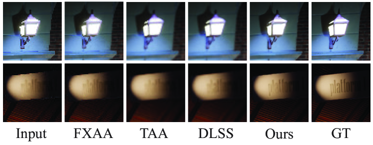
(a) Qualitative comparison.

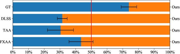
(b) User study results of preference.

Figure 8: Comparison against off-the-shelf methods.

Conclusion

In this paper, we propose a novel unified Space-Time Super-Sampling (STSS) framework to improve the resolution and frame rate. We handle aliasing and occluded regions unified as reshading regions and propose Random Reshading Masking and Efficient Reshading Module. Extensive experiments demonstrate that our method can generate better results and inference much faster than previous methods. It can inspire future research on the STSS problem.

Appendix

Comparison on Single Tasks

To demonstrate the benefit of a unified framework, we perform a conceptual experiment which ignores the pipeline and compares supersampling (Sup.) methods only on SFs and frame generation (Gen.) only on EFs. The frame generation methods are evaluated on the original 540P for a fair comparison. Tab. 7 shows that we have an average 0.76dB PSNR advantage on each task.

Sup.	PSNR $\uparrow$	SSIM $\uparrow$	Gen.	PSNR $\uparrow$	SSIM $\uparrow$
EDVR	30.45	0.911	RIFE	32.21	0.931
NSRR	34.29	0.953	ExtraNet	33.88	0.950
Ours	35.02	0.957	Ours	34.67	0.955

Table 7: Quantitative comparison on single tasks.

Comparison with Two Stage Swapped

In the main paper, we experiment with the assumption that the two stages of supersampling and interpolation/extrapolation have fixed order. The interpolation/extrapolation must be performed before supersampling. Therefore, we further swapped the two stages’ order and showed the average metrics on the Lewis scene in Tab. 8. The performance of two-stage methods is even more degraded than in the previous setting. One possible reason is that the HR G-buffers are unavailable in the second stage, and only the LR G-buffers can be used instead, which is unfavorable for extrapolation. The generated artifacts will accumulate when a frame is supersampled and then interpolated.

Model	PSNR $\uparrow$	SSIM $\uparrow$	LPIPS $\downarrow$
EDVR+RIFE	29.66	0.8986	0.1349
NSRR+RIFE	33.25	0.9400	0.0847
EDVR+ExtraNet	32.13	0.9297	0.1110
NSRR+ExtraNet	34.05	0.9508	0.0848
STSSNet(Ours)	34.87	0.9559	0.0190

Table 8: Quantitative comparison of two-phase exchange. We swap the two stages to demonstrate the effect of stage order.

Comparison with Fine-tuned Models

Since the video-based methods are usually pretrained on a larger dataset, we also compare the performance of finetuned models on Lewis in Tab. 9. We use the official models of RIFE, EDVR, and ZoomingSloMo as base models and finetune them for 100 epochs. Since NSRR and ExtraNet lack pre-trained models of large datasets, we train them from scratch to align with our method. Our method maintains the performance advantage.

Model	PSNR $\uparrow$	SSIM $\uparrow$	LPIPS $\downarrow$
RIFE+EDVR	34.47/32.73	0.949/0.923	0.023/0.032
RIFE+NSRR	34.14/32.35	0.951/0.924	0.022/0.037
ExtraNet+EDVR	34.49/34.30	0.949/0.947	0.023/0.024
ExtraNet+NSRR	34.29/33.87	0.953/0.951	0.080/0.089
ZoomingSloMo	34.50/31.51	0.944/0.917	0.024/0.039
Ours	35.02/34.72	0.957/0.955	0.018/0.020

Table 9: Quantitative comparison with fine-tuned video methods.

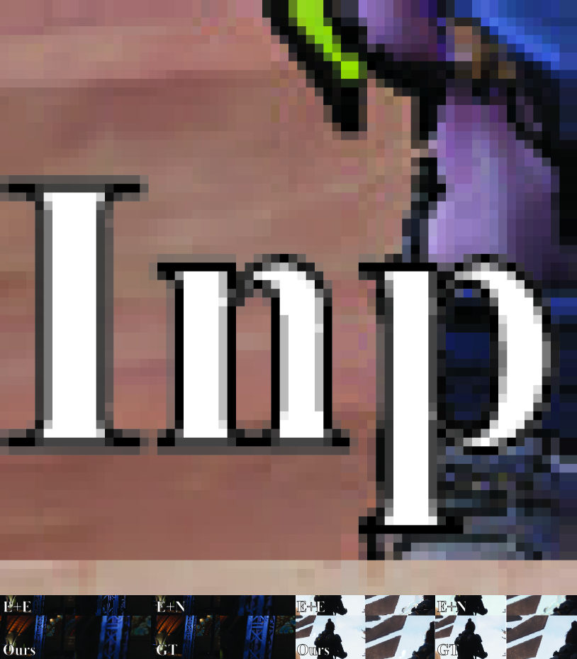
Figure 9: Qualitative comparison with SOTA methods. The first row is the example frames from the different scenes, and the following rows are cropped from the red triangle. From up to down and left to right: Input, Zooming-SloMo, RIFE+EDVR, RIFE+NSRR, ExtraNet+EDVR, ExtraNet+NSRR, Ours, GT. The black region in the input is the warping occlusion. Please zoom in for a better view.

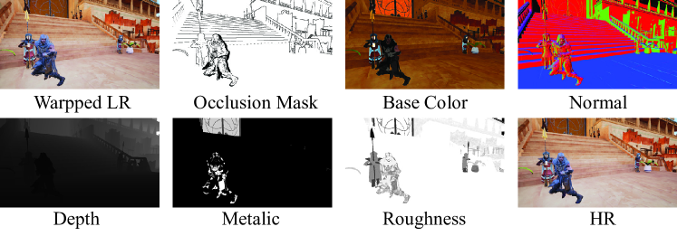
Figure 10: Visualization of the generated dataset. The G-buffer is composed of base color, normal, depth, metallic, and roughness. The warped LRs differ for extrapolating frames(EF) and supersampling frames(SF). EFs are warped in the future frame by motion vectors, but the SFs are warped to the present frame.

More Visualization

Fig. 9 shows more qualitative comparison in Lewis, SunTemple, Subway, and Arena scenes. Our method achieves better quality in the details.

Fig. 10 show the visualization of the datasets. G-buffer for network input comprises base color, metallic, roughness, depth, and normal.

References

- Akeley (1993) Akeley, K. 1993. Reality engine graphics. In Proceedings of the 20th annual conference on Computer graphics and interactive techniques, 109–116.
- Andrew Edelsten and Patney (2019) Andrew Edelsten, P. J.; and Patney, A. 2019. Truly next-gen: Adding deep learning to games and graphics.
- Briedis et al. (2021) Briedis, K. M.; Djelouah, A.; Meyer, M.; McGonigal, I.; Gross, M.; and Schroers, C. 2021. Neural frame interpolation for rendered content. ACM Transactions on Graphics (TOG), 40(6): 1–13.
- Briedis et al. (2023) Briedis, K. M.; Djelouah, A.; Ortiz, R.; Meyer, M.; Gross, M. H.; and Schroers, C. 2023. Kernel-Based Frame Interpolation for Spatio-Temporally Adaptive Rendering. ACM SIGGRAPH 2023 Conference Proceedings.
- Chowdhury et al. (2022) Chowdhury, H.; Kawiak; Robert, R.; de Boer; Ferreira, G.; ; and Xavier, L. 2022. Intel XeSS – an AI based Super Sampling solution for Real-time Rendering.
- Ding et al. (2021) Ding, T.; Liang, L.; Zhu, Z.; and Zharkov, I. 2021. Cdfi: Compression-driven network design for frame interpolation. In Proceedings of the IEEE/CVF Conference on Computer Vision and Pattern Recognition, 8001–8011.
- EpicGames (2020) EpicGames. 2020. Temporal Anti-Aliasing Upsample.
- Geng et al. (2022) Geng, Z.; Liang, L.; Ding, T.; and Zharkov, I. 2022. RSTT: Real-time Spatial Temporal Transformer for Space-Time Video Super-Resolution. In Proceedings of the IEEE/CVF Conference on Computer Vision and Pattern Recognition, 17441–17451.
- GPUOpen-Effects (2022) GPUOpen-Effects. 2022. FidelityFX-FSR2. https://github.com/GPUOpen-Effects/FidelityFX-FSR2.
- GPUOpen-Effects (2023) GPUOpen-Effects. 2023. FidelityFX-FSR2. https://github.com/GPUOpen-Effects/FidelityFX-FSR2.
- Guo et al. (2021) Guo, J.; Fu, X.; Lin, L.; Ma, H.; Guo, Y.; Liu, S.; and Yan, L.-Q. 2021. ExtraNet: real-time extrapolated rendering for low-latency temporal supersampling. ACM Transactions on Graphics (TOG), 40(6): 1–16.
- Guo et al. (2022) Guo, Y.-X.; Chen, G.; Dong, Y.; and Tong, X. 2022. Classifier Guided Temporal Supersampling for Real-time Rendering. In Computer Graphics Forum, volume 41, 237–246. Wiley Online Library.
- Hu et al. (2023) Hu, M.; Jiang, K.; Nie, Z.; Zhou, J.; and Wang, Z. 2023. Store and fetch immediately: Everything is all you need for space-time video super-resolution. In Proceedings of the AAAI Conference on Artificial Intelligence, volume 37, 863–871.
- Huang et al. (2022) Huang, Z.; Zhang, T.; Heng, W.; Shi, B.; and Zhou, S. 2022. Real-Time Intermediate Flow Estimation for Video Frame Interpolation. In Proceedings of the European Conference on Computer Vision (ECCV).
- Kajiya (1986) Kajiya, J. T. 1986. The rendering equation. In Proceedings of the 13th annual conference on Computer graphics and interactive techniques, 143–150.
- Karis (2014) Karis, B. 2014. High-quality Temporal Supersampling. SIGGRAPH (Advances in Real-Time Rendering).
- Li et al. (2023) Li, G.; Ji, J.; Qin, M.; Niu, W.; Ren, B.; Afghah, F.; Guo, L.; and Ma, X. 2023. Towards High-Quality and Efficient Video Super-Resolution via Spatial-Temporal Data Overfitting. arXiv preprint arXiv:2303.08331.
- Li et al. (2018) Li, Z.; Bampis, C.; Novak, J.; Aaron, A.; Swanson, K.; Moorthy, A.; and Cock, J. 2018. VMAF: The journey continues. Netflix Technology Blog, 25.
- Li et al. (2022) Li, Z.; Marshall, C. S.; Vembar, D. S.; and Liu, F. 2022. Future Frame Synthesis for Fast Monte Carlo Rendering. In Graphics Interface 2022.
- Liang et al. (2022) Liang, J.; Cao, J.; Fan, Y.; Zhang, K.; Ranjan, R.; Li, Y.; Timofte, R.; and Van Gool, L. 2022. Vrt: A video restoration transformer. arXiv preprint arXiv:2201.12288.
- Lin and Burnes (2022) Lin, H. C.; and Burnes, A. 2022. NVIDIA DLSS 3: AI-Powered Performance Multiplier Boosts Frame Rates By Up To 4X.
- Lottes (2009) Lottes, T. 2009. Fxaa. White paper, Nvidia, Febuary, 2.
- Oprea et al. (2020) Oprea, S.; Martinez-Gonzalez, P.; Garcia-Garcia, A.; Castro-Vargas, J. A.; Orts-Escolano, S.; Garcia-Rodriguez, J.; and Argyros, A. 2020. A review on deep learning techniques for video prediction. IEEE Transactions on Pattern Analysis and Machine Intelligence.
- Plack et al. (2023) Plack, M.; Briedis, K. M.; Djelouah, A.; Hullin, M. B.; Gross, M.; and Schroers, C. 2023. Frame Interpolation Transformer and Uncertainty Guidance. In Proceedings of the IEEE/CVF Conference on Computer Vision and Pattern Recognition, 9811–9821.
- Reshetov (2009) Reshetov, A. 2009. Morphological antialiasing. In Proceedings of the Conference on High Performance Graphics 2009, 109–116.
- Ronneberger, Fischer, and Brox (2015) Ronneberger, O.; Fischer, P.; and Brox, T. 2015. U-net: Convolutional networks for biomedical image segmentation. In International Conference on Medical image computing and computer-assisted intervention, 234–241. Springer.
- Schneider (2020) Schneider, S. 2020. Introducing NVIDIA Reflex: Optimize and Measure Latency in Competitive Games.
- Shi et al. (2023) Shi, X.; Wang, L.; Wu, J.; Ke, W.; and Lam, C.-T. 2023. Locomotion-aware Foveated Rendering. In 2023 IEEE Conference Virtual Reality and 3D User Interfaces (VR), 471–481. IEEE.
- Simonyan and Zisserman (2014) Simonyan, K.; and Zisserman, A. 2014. Very deep convolutional networks for large-scale image recognition. arXiv preprint arXiv:1409.1556.
- Teed and Deng (2020) Teed, Z.; and Deng, J. 2020. Raft: Recurrent all-pairs field transforms for optical flow. In Computer Vision–ECCV 2020: 16th European Conference, Glasgow, UK, August 23–28, 2020, Proceedings, Part II 16, 402–419. Springer.
- Thomas et al. (2022) Thomas, M. M.; Liktor, G.; Peters, C.; Kim, S.; Vaidyanathan, K.; and Forbes, A. G. 2022. Temporally Stable Real-Time Joint Neural Denoising and Supersampling. Proceedings of the ACM on Computer Graphics and Interactive Techniques, 5(3): 1–22.
- Thomas et al. (2020) Thomas, M. M.; Vaidyanathan, K.; Liktor, G.; and Forbes, A. G. 2020. A reduced-precision network for image reconstruction. ACM Transactions on Graphics (TOG), 39: 1 – 12.
- Wang et al. (2019) Wang, X.; Chan, K. C.; Yu, K.; Dong, C.; and Change Loy, C. 2019. Edvr: Video restoration with enhanced deformable convolutional networks. In Proceedings of the IEEE/CVF Conference on Computer Vision and Pattern Recognition Workshops, 0–0.
- Wang et al. (2004) Wang, Z.; Bovik, A. C.; Sheikh, H. R.; and Simoncelli, E. P. 2004. Image quality assessment: from error visibility to structural similarity. IEEE transactions on image processing, 13(4): 600–612.
- Wu, Wen, and Chen (2022) Wu, Y.; Wen, Q.; and Chen, Q. 2022. Optimizing Video Prediction via Video Frame Interpolation. In Proceedings of the IEEE/CVF Conference on Computer Vision and Pattern Recognition, 17814–17823.
- Xiang et al. (2020) Xiang, X.; Tian, Y.; Zhang, Y.; Fu, Y.; Allebach, J. P.; and Xu, C. 2020. Zooming slow-mo: Fast and accurate one-stage space-time video super-resolution. In Proceedings of the IEEE/CVF conference on computer vision and pattern recognition, 3370–3379.
- Xiao et al. (2020) Xiao, L.; Nouri, S.; Chapman, M.; Fix, A.; Lanman, D.; and Kaplanyan, A. 2020. Neural supersampling for real-time rendering. ACM Transactions on Graphics (TOG), 39(4): 142–1.
- Zeng et al. (2021) Zeng, Z.; Liu, S.; Yang, J.; Wang, L.; and Yan, L.-Q. 2021. Temporally Reliable Motion Vectors for Real-time Ray Tracing. In Computer Graphics Forum, volume 40, 79–90. Wiley Online Library.
- Zhang, Titov, and Sennrich (2021) Zhang, B.; Titov, I.; and Sennrich, R. 2021. Sparse attention with linear units. arXiv preprint arXiv:2104.07012.
- Zhang et al. (2018) Zhang, R.; Isola, P.; Efros, A. A.; Shechtman, E.; and Wang, O. 2018. The Unreasonable Effectiveness of Deep Features as a Perceptual Metric. In 2018 IEEE/CVF Conference on Computer Vision and Pattern Recognition, 586–595.
- Zhong et al. (2020) Zhong, Z.; Zheng, L.; Kang, G.; Li, S.; and Yang, Y. 2020. Random erasing data augmentation. In Proceedings of the AAAI conference on artificial intelligence, volume 34, 13001–13008.
- Zhou et al. (2021) Zhou, C.; Lu, Z.; Li, L.; Yan, Q.; and Xue, J.-H. 2021. How Video Super-Resolution and Frame Interpolation Mutually Benefit. In Proceedings of the 29th ACM International Conference on Multimedia, 5445–5453.