Age-Threshold Slotted ALOHA for Optimizing Information Freshness in Mobile Networks

Abstract

We optimize the Age of Information (AoI) in mobile networks using the age-threshold slotted ALOHA (TSA) protocol. The network comprises multiple source-destination pairs, where each source sends a sequence of status update packets to its destination over a shared spectrum. The TSA protocol stipulates that a source node must remain silent until its AoI reaches a predefined threshold, after which the node accesses the radio channel with a certain probability. Using stochastic geometry tools, we derive analytical expressions for the transmission success probability, mean peak AoI, and time-average AoI. Subsequently, we obtain closed-form expressions for the optimal update rate and age threshold that minimize the mean peak and time-average AoI, respectively. In addition, we establish a scaling law for the mean peak AoI and time-average AoI in mobile networks, revealing that the optimal mean peak AoI and time-average AoI increase linearly with the deployment density. Notably, the growth rate of time-average AoI under TSA is half of that under conventional slotted ALOHA. When considering the optimal mean peak AoI, the TSA protocol exhibits comparable performance to the traditional slotted ALOHA protocol. These findings conclusively affirm the advantage of TSA in reducing higher-order AoI, particularly in densely deployed networks.

I Introduction

Timeliness has emerged as a fundamental prerequisite for Internet-of-Things (IoT) services, encompassing various applications such as autonomous driving, smart factory operations, and intelligent healthcare. Acquiring timely updates from massively deployed sensors is crucial for making prompt and accurate decisions in these applications[1].

To assess the timeliness of delivered messages, the notion of Age of Information (AoI) has been proposed in [2], where the authors showed that minimizing AoI is fundamentally different from optimizing conventional metrics such as delay or throughput. As a result, plenty of research efforts have been devoted to ensuring timely information delivery over communication networks. This paper employs the age-threshold slotted ALOHA (TSA), a variant of the classic ALOHA protocol, to enhance AoI in random access networks. We study the minimization of AoI through the lens of the signal-to-interference-plus-noise ratio (SINR) model, by optimally adjusting the parameters of TSA according to the network configuration. The resultant scheme has low complexity and is particularly relevant to large-scale wireless systems.

I-A Related Works

In the early stages of AoI analysis for large-scale networks, many researchers adopted the traditional analytical framework of slotted ALOHA. For example, [3] characterized and optimized the average AoI by optimal tuning the channel access probability. [4] optimized the peak AoI using First-Come-First-Serve (FCFS) and Last-Come-First-Serve (LCFS) strategies, showing that with optimal packet arrival rate and channel access probability, the peak AoI scales linearly with the number of access nodes. [5] considered a multi-channel ALOHA network, enhancing AoI performance via joint radio access control and resource allocation. [6] explores the average AoI performance in a heterogeneous random access network where stochastic arrival nodes coexist with generate-at-will nodes. These efforts have alleviated the performance bottlenecks of the AoI metric in large-scale networks. However, the primary objective behind the conventional slotted ALOHA was to mitigate channel contention, thereby enhancing transmission success probability or throughput. It was not explicitly designed to cater to the distinct attributes of the AoI metric. Hence, it becomes essential to explore random access protocols that closely align with the attributes of the AoI metric.

When reconsidering the design of an age-aware random access network, it becomes essential to (a) mitigate network interference, (b) minimize the waiting time for information packets within the transmitter system, and (c) ensure equalization of the update packet reception intervals. A straightforward strategy to address these needs is to prioritize nodes with lower timeliness for updates, allowing nodes with higher information freshness to remain silent temporarily. Based on this idea, several works [7, 8, 9, 10, 11] extended the slotted ALOHA (SA) into an age-aware variant. Specifically, a threshold-based age-dependent random access protocol was proposed in [7, 8, 11, 12], where each node accesses the channel only when its instantaneous AoI exceeds a predetermined threshold. A distributed transmission strategy was proposed in [9] based on the age gain, defined as the reduction of instantaneous AoI when packets are successfully delivered. An Index-Prioritized Random Access scheme was proposed in [10], where nodes access the channel according to their indices that reflect the urgency of the update. The function of irregular repetition slotted ALOHA (IRSA) on various AoI performance metrics has been demonstrated in [12].

The aforementioned research endeavors predominantly concentrate on the single-cell setting, where multiple nodes transmit data to a central access point. However, it is imperative to consider the ad-hoc network scenario for a more comprehensive understanding. Another noteworthy aspect is that the interference in the above references is modeled by the collision model[13], wherein concurrent transmissions always lead to communication failures. Such a model neglects essential physical elements in wireless channels, such as fading, path loss, and spatial network topology, oversimplifying the co-channel interference effects. In contrast, the SINR model is preferable to the update packet verdict on the receiver end, as it can adequately account for these critical features in the ad-hoc network scenario.

Consequently, a line of recent studies has been carried out, analyzing and optimizing AoI in wireless networks on the basis of the SINR model[14, 15, 16, 17, 18, 19, 20, 21, 22, 23, 24, 25, 26]. Specifically, the upper and lower bounds of the time-average AoI in Poisson bipolar networks are provided in [14] based on the favorable/dominant system argument, and the upper bound is improved by reconstruction of the dominant system in [15]. The authors in [16] derived the average peak AoI with different packet arrival patterns, i.e., the time-triggered and event-triggered traffic for large-scale wireless networks, while the authors in [17] and [18] analyze the AoI statistics under different buffer sizes and package management disciplines. The authors in [19] present a comprehensive study on the interplay between throughput and AoI in a cellular-based IoT network. Explicit optimal expression of peak AoI of slotted ALOHA, and its optimal parameters are derived in [20], the distinctions and similarities between the optimal parameters for the peak AoI and average AoI are extensively discussed in [21]. The energy-AoI tradeoff is further explored in [22]. The authors in [23] examine the AoI performance of random access networks under frame-slotted ALOHA protocol. Locally adaptive strategies for optimizing AoI have been studied in [24], [25], and [26], where the channel access probability, update rate, and transmit power at each node are adjusted according to the local communication environment to minimize AoI.

The existing results primarily pertain to the conventional slotted ALOHA protocol, whilst the effects of the age threshold remain unexplored. Although a recent work [27] has investigated the effect of TSA on AoI performance in static Poisson bipolar networks, the analysis involve complicated expressions of the SINR meta distribution, prohibiting it from optimizing TSA to reap the full potential of this protocol. In this paper, we consider the AoI optimization under TSA in a high mobility case, with which we can establish tractable analysis and obtain closed-form results that provide insights into network designs.

I-B Contributions

The main contributions of this paper are summarized below.

• We develop a mathematical framework for analyzing the impact of the TSA protocol on the AoI performance of random access networks. We establish a fixed-point equation to characterize the transmission success probability, encompassing key features such as the update rate, age threshold, channel fading, deployment density, and co-channel interference.

• We derive analytical expressions of the mean peak AoI and time-average AoI over the typical link. Our analysis culminates in an optimization strategy to minimize these AoI metrics, achieved by a joint optimization of the update rate and age threshold. Specifically, we investigate the performance limits of the mean peak AoI under TSA protocol and identify the corresponding parameter pairs that enable its minimization. We also propose an alternative iterative algorithm to achieve the optimal parameter configuration that minimizes the time-average AoI. Additionally, we derive closed-form approximations for these optimal parameters, which are asymptotically accurate.

• We establish a scaling law of AoI in random access networks. Notably, it reveals that although the optimal mean peak AoI and time-average AoI increase linearly with the deployment density, the growth rate of time-average AoI under TSA protocol is only half of that under conventional slotted ALOHA.

• Considering the inherent instability of ALOHA-like networks, especially under conditions of high interference levels and traffic load, we propose parameter tuning strategies for both mean peak AoI and time-average AoI in the presence of a bistable region, aiming to bolster the robustness of the TSA protocol network.

TABLE I: key notations

Notations	Definition	Notations	Definition
$\lambda$	Spatial deployment density	$\hat{\Delta}_{0}$	Mean peak AoI of typical link
$r$	Transceiver distance	$\bar{\Delta}_{0}$	Time-average AoI of typical link
$\eta$	Update rate	$\hat{\eta}^{*}_{|A}$	Optimal update rate (Fixed $A$, mean peak AoI)
$A$	Age-threshold	$\hat{A}^{*}_{|\eta}$	Optimal age-threshold (Fixed $\eta$, mean peak AoI)
$\alpha$	Path-loss fading coefficient	$(\hat{A}^{*},\hat{\eta}^{*})$	Optimal age-threshold $\&$ update rate (mean peak AoI)
$\rho$	SNR	$\bar{\eta}^{*}_{|A}$	Optimal update rate (Fixed $A$, time-average AoI)
$\theta$	Decoding SINR threshold	$\bar{A}^{*}_{|\eta}$	Optimal update rate (Fixed $\eta$, time-average AoI)
$p_{\mathrm{s}}$	Transmission success probability	$(\bar{A}^{*},\bar{\eta}^{*})$	Optimal age-threshold $\&$ update rate (time-average AoI)
$p_{\mathrm{s}}^{L}$	$p_{\mathrm{s}}$ in low efficiency state	$\hat{\Delta}_{0}^{*}$	Optimal mean peak AoI
$p_{\mathrm{s}}^{H}$	$p_{\mathrm{s}}$ in high efficiency state	$\bar{\Delta}_{0}^{*}$	Optimal time-average AoI

II system model

II-A Spatial Configuration

We consider a random access network comprised of source-destination pairs. The source nodes are scattered according to a homogeneous Poisson point process (HPPP) $\Phi_{\mathrm{s}}=\{X_{i}\}_{i=1}^{\infty}$ of density $\lambda$. The main notations used throughout this article are summarized in Table I. Each source is paired with a destination situated in distance $r$ and oriented in a random direction. According to the displacement theorem[28][29], locations of the destination nodes constitute an independent HPPP $\Phi_{\mathrm{d}}$ of the same density. We add a receiver at the origin to the point process $\Phi_{\mathrm{d}}$. We also add its tagged transmitter, denoted by $X_{0}$, to the point process $\Phi_{\mathrm{s}}$. We refer to this link pair as the typical one. Based on Slivnyak’s theorem[28][29], we can concentrate on analyzing the performance of the typical link. A sequence of status information is generated at each source, encapsulated into information packets, and transmitted over a shared spectrum. When a source node sends out information packets, it transmits at a fixed power. We assume the channel between any pair of nodes is affected by the Rayleigh fading with a unit mean, which varies independently across time slots, and path loss that follows the power law. We also assume the received signal is subjected to white Gaussian thermal noise.

II-B Temporal Pattern

In this network, the time is slotted into equal-length intervals, and the transmission of each packet occupies one slot. We assume the network is synchronized. Each source adopts the generate-at-will policy for the status updating. Particularly, if a node decides to transmit, it will generate a new sample at the beginning of the time slot and send the information packet to the destination immediately. By the end of the same time slot, the packet is successfully decoded if the received SINR exceeds a decoding threshold; otherwise, the transmission fails, and in that case, the packet is dropped. The delivery of packets, therefore, incurs a delay of one time slot. Additionally, the positions of the links vary according to the high mobility random walk model[20, 30], i.e., spatial locations of the link pairs are (re)generated independently in each time slot according to the same Poisson bipolar network model.

II-C Transmission Protocol

This work employs the TSA protocol for status updating. Specifically, every source node stays inactive until its AoI reaches a predefined threshold, denoted by $A$, upon which the source node turns on the status updating mode: it generates a fresh sample with probability $\eta$ at the beginning of each time slot, encapsulates that information into a packet, and immediately sends it to the destination. If the received SINR surpasses a decoding threshold $\theta$, the transmission succeeds; the receiver then feeds back an ACK to the source and the age is reset to one. Otherwise, the source will generate a new sample in the next time slot with probability $\eta$. This probability is usually referred to as the update rate.

II-D Performance Metric

We put the main focus on the notion of AoI in this paper. As depicted in Fig. 1, AoI grows linearly with time in the absence of new updates at the destination, and it drops to the time elapsed since the generation of the latest packet received. Formally, the age evolution process over the typical link can be written as follows

$$\Delta_{0}(t)=t-G_{0}(t),$$ (1)

where $G_{0}(t)$ denotes the generation time of the latest packet successfully delivered over this link.

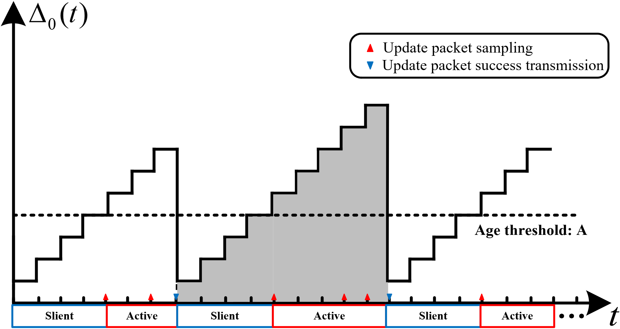
Figure 1: An illustration of the time evolution of the age of information over the link under consideration.

In this paper, we use the mean peak AoI and time-average AoI over the typical link as our performance metrics, defined respectively as

$$\hat{\Delta}_{0}=\lim_{N\rightarrow\infty}\frac{1}{N}\sum_{n=1}^{N}\Delta_{0}(T_{0}(n))$$ (2)

where $T_{0}(n)$ denotes the time slot at which the $n$-th packet is successfully delivered, and

$$\bar{\Delta}_{0}=\lim_{T\to\infty}\frac{1}{T}\sum_{t=1}^{T}\Delta_{0}(t).$$ (3)

Since the point processes formed by the TSA protocol still exhibit ergodicity and stationarity, the statistical characteristics of AoI performance for the typical link are identical to those of the other links.

III AoI Analysis

III-A SINR at the Typical Receiver

Since all the source nodes use the same spectrum for packet delivery, each transmission would be affected by others owing to co-channel interference. As such, at the typical destination, the received SINR at time slot $t$ is

$$\mathrm{SINR}_{0}(t)=\frac{h_{00}(t)r^{-\alpha}}{\sum_{i\neq 0}h_{i0}(t)v_{i}(t)||X_{i}||^{-\alpha}+\rho^{-1}},$$ (4)

where $h_{i0}(t)\sim\exp(1)$ represents the small-scale fading between transmitter $i$ and the typical receiver, $\alpha$ is the path-loss exponent, $\|\cdot\|$ stands for the Euclidean norm, $\rho$ denotes the signal-to-noise ratio (SNR), and $v_{i}(t)$ is a binary function, where $v_{i}(t)=1$ indicates that transmitter $i$ initiates a packet transmission at time slot $t$, and $v_{i}(t)=0$ otherwise.

III-B Transmission Success Probability

According to the transmission policy, an information packet is successfully delivered if the received SINR exceeds a decoding threshold $\theta$. Therefore, the probability of successfully transmitting a packet from the typical source node can be written as

$$p_{\mathrm{s}}(t)=\mathbb{P}\left(\mathrm{SINR}_{0}(t)>\theta\right).$$ (5)

Under the high mobility random walk model, the received $\text{SINR}_{i}(t)$ of each transmitter $i$, $i\in\mathbb{N}$, is independent and identically distributed (i.i.d.) across time $t$. By symmetry, the transmission success probability is also identical across the transmitters. As such, we drop the time index from $p_{\mathrm{s}}(t)$ in the sequel. The following theorem provides a formal characterization of this quantity.

Theorem 1.

The transmission success probability under TSA is given by the following fixed-point equation

$$p_{\mathrm{s}}=\exp\left(-\frac{\lambda c\eta r^{2}}{1+A\eta p_{\mathrm{s}}}-\frac{\theta r^{\alpha}}{\rho}\right),$$ (6)

in which

$$c=\pi\theta^{\frac{2}{\alpha}}\Gamma\left(1-\frac{2}{\alpha}\right)\Gamma\left(1+\frac{2}{\alpha}\right),$$ (7)

where $\Gamma(\cdot)$ denotes the Gamma function [31].

Proof:

Please see Appendix A. ∎

The parameter $c$ in (6) reflects the level of spatial contention [32], measuring the network’s capability of spatial reuse by quantifying how fast the transmission success probability deteriorates when the interferers’ density increases.

Remark 1.

In the static deployment case [27], the transmission success probability of each source differs from node to node. Consequently, it requires deriving the SINR meta distribution to characterize the link performance. Although this approach provides a fine-grained perspective for network analysis, it often leads to complex analytical expressions that hinder the exploration of AoI limits. In contrast, the mobile network model considered by this paper mitigates the influence of spatial correlations among the nodes, enabling tractable results that provide useful network design guidelines, which will be detailed in the subsequent sections.

The fixed-point equation (6) captures the spatial-temporal interactions amongst the source nodes across the network. And solutions to such an equation can be obtained via fixed-point iterations. Next, we investigate the conditions of different distributions of roots of (6).

Corollary 1.

The fixed-point equation in (6) has three non-zero roots, $0<p_{\mathrm{s}}^{L}<p_{\mathrm{s}}^{M}<p_{\mathrm{s}}^{H}<1$, if

$$\lambda cr^{2}>\frac{4}{\eta}$$ (8)

and

$$A_{l}<A<A_{h},$$ (9)

where $A_{l}$ and $A_{h}$ are given respectively as follows

$$A_{l}=\frac{\lambda cr^{2}\left(\frac{1}{2}+\sqrt{\frac{1}{4}-\frac{1}{\lambda cr^{2}\eta}}\right)-\frac{1}{\eta}}{\exp\left(-\frac{\theta r^{\alpha}}{\rho}-\frac{1}{\frac{1}{2}+\sqrt{\frac{1}{4}-\frac{1}{\lambda cr^{2}\eta}}}\right)},$$ (10)

$$A_{h}=\frac{\lambda cr^{2}\left(\frac{1}{2}-\sqrt{\frac{1}{4}-\frac{1}{\lambda cr^{2}\eta}}\right)-\frac{1}{\eta}}{\exp\left(-\frac{\theta r^{\alpha}}{\rho}-\frac{1}{\frac{1}{2}-\sqrt{\frac{1}{4}-\frac{1}{\lambda cr^{2}\eta}}}\right)}.$$ (11)

When $A=A_{l}$ or $A=A_{h}$, (6) has two solutions; otherwise, (6) has a unique solution.

Proof:

Please see Appendix B. ∎

Remark 2.

In the scenario that (6) has three non-zero roots, the feasible ranges of $p_{\mathrm{s}}^{L}$ and $p_{\mathrm{s}}^{H}$ are given respectively as follows:

$$p_{\mathrm{s}}^{L}\in\left(0,~{}\exp\left(-\tfrac{\theta r^{\alpha}}{\rho}-\tfrac{1}{\frac{1}{2}-\sqrt{\frac{1}{4}-\frac{1}{\lambda cr^{2}\eta}}}\right)\right),$$ (12)

$$p_{\mathrm{s}}^{H}\in\left(\exp\left(-\tfrac{\theta r^{\alpha}}{\rho}-\tfrac{1}{\frac{1}{2}+\sqrt{\frac{1}{4}-\frac{1}{\lambda cr^{2}\eta}}}\right),~{}1\right).$$ (13)

To determine whether all the roots of the fixed-point equation are steady-state points, we need the trajectory analysis of the transmission success probability $p_{\mathrm{s}}$. We take an approximate approach similar to the one proposed in [33].

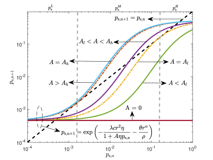
Figure 2: Approximate trajectory of $p_{\mathrm{s,n}}$. Spatial deployment density $\lambda=0.15$, update rate $\eta=1$, decoding threshold $\theta=0~{}\text{dB}$, SNR $\rho=20~{}\text{dB}$, path-loss exponent $\alpha=3.8$, and transceiver distance $r=3$.

Specifically, we denote by $p_{\mathrm{s},n}$ the estimation of transmission success probability after the $n$th iteration, which is the input of the $(n+1)$th iteration. More precisely, the iteration process can be expressed as follows

$$p_{\mathrm{s},n+1}=\exp\left(-\frac{\lambda c\eta r^{2}}{1+A\eta p_{\mathrm{s},n}}-\frac{\theta r^{\alpha}}{\rho}\right).$$ (14)

A pictorial example is provided in Fig. 2, where we set the parameters that satisfy $\lambda cr^{2}>\frac{4}{\eta}$ and showcase six distinct curves, arranged based on the value of the age threshold. Specifically, they are: $(i)$ $A=0$, $(ii)$ $A=10\in(0,A_{l})$, $(iii)$ $A=A_{l}\approx 31$, $(iv)$ $A=50\in(A_{l},A_{h})$, $(v)$ $A=A_{h}\approx 135$, and $(vi)$ $A=150\in(A_{h},+\infty)$.

Let us take the case of $A=50\in(A_{l},A_{h})$ as an example to demonstrate the analytical approach. In this case, the region of $p_{\mathrm{s},n}$ has four possible scenarios: (1) $0<p_{\mathrm{s},n}<p_{\mathrm{s}}^{L}$; (2) $p_{\mathrm{s}}^{L}<p_{\mathrm{s},n}<p_{\mathrm{s}}^{M}$; (3) $p_{\mathrm{s}}^{M}<p_{\mathrm{s},n}<p_{\mathrm{s}}^{H}$; and (4) $p_{\mathrm{s}}^{H}<p_{\mathrm{s},n}<1$. In the first and second scenarios, $p_{\mathrm{s},n}$ will gradually approach $p_{\mathrm{s}}^{L}$. In contrast, $p_{\mathrm{s},n}$ tends toward $p_{\mathrm{s}}^{H}$ in the third and fourth cases. As such, in this example, there are two candidate points, namely, $p_{\mathrm{s}}^{L}$ and $p_{\mathrm{s}}^{H}$, that $p_{\mathrm{s},n}$ can converge to. In a similar vein, we can show that $p_{\mathrm{s},n}$ only converges to $p_{\mathrm{s}}^{H}$ (or $p_{\mathrm{s}}^{L}$) in other cases.

Correspondingly, we define the following stable regions for the solutions:

• Bistable region:

  $$\mathcal{B}=\left\{\left(\lambda,\theta,r,\alpha,\rho,A,\eta\right)\big{|}\lambda cr^{2}>\frac{4}{\eta},A_{l}<A<A_{h}\right\},$$

  in which the network has two steady-state points $p_{\mathrm{s}}^{L}$ and $p_{\mathrm{s}}^{H}$.

• Monostable region: $\mathcal{M}=\bar{\mathcal{B}}$ (i.e., the complement of set $\mathcal{B}$); in this case, the network has one steady state point $p_{\mathrm{s}}^{H}$(or $p_{\mathrm{s}}^{L}$).

The following corollary summarizes the properties of the steady-state points in terms of the configuration parameters.

Corollary 2.

The steady-state transmission success probabilities $p_{\mathrm{s}}^{L}$ and $p_{\mathrm{s}}^{H}$are increasing functions of the age threshold $A$, while they decrease in terms of the spatial deployment density $\lambda$ and update rate $\eta$.

Proof:

Please see Appendix C. ∎

It is intuitive that in densely deployed networks, the transmission success probability will benefit (more) from the TSA protocol due to its capability in mitigating channel contention. This can also be observed from Fig. 2 by comparing the value of transmission success probability at $A=0$ with those at $A>0$.

III-C AoI Statistics

Using the transmission success probability, we can derive closed-form expressions for the mean peak AoI and time-average AoI as follows.

Theorem 2.

Under the TSA protocol, the mean peak AoI over the typical link is

$$\hat{\Delta}_{0}=A+\frac{1}{\eta p_{\mathrm{s}}},$$ (15)

and the time-average AoI is

$$\bar{\Delta}_{0}=\frac{A+1}{2}+\frac{1}{\eta p_{\mathrm{s}}}-\frac{A+1}{2\left(1+A\eta p_{\mathrm{s}}\right)},$$ (16)

where $p_{\mathrm{s}}$ is given in (6).

Proof:

Please see Appendix D. ∎

Leveraging the above theorem, we can investigate different regimes of the age threshold to demystify its influence on the AoI performance. Firstly, if we set the age threshold $A$ to be zero, the results in Theorem 2 reduce to the mean peak AoI and time-average AoI in large-scale networks under the conventional slotted ALOHA (SA) protocol, i.e.,

$$\hat{\Delta}^{\mathrm{SA}}_{0}=\bar{\Delta}^{\mathrm{SA}}_{0}=\frac{\exp\left(\lambda cr^{2}\eta+\theta r^{\alpha}\rho^{-1}\right)}{\eta}.$$ (17)

Consequently, we can compare the AoI achieved under the SA and TSA protocols to identify the operating regimes where TSA outperforms SA.

We first compare the mean peak AoI attained under the SA and TSA protocols for $A>0$, which yields

$$\hat{\Delta}_{0}^{\mathrm{SA}}-\hat{\Delta}_{0}^{\mathrm{TSA}}=\frac{1}{\eta p_{\mathrm{s}}^{\mathrm{SA}}}-\left(A+\frac{1}{\eta p_{\mathrm{s}}^{\mathrm{TSA}}}\right)$$

$$=\frac{\left(\exp\left(\lambda cr^{2}\eta\right)-\exp\left(\frac{\lambda cr^{2}\eta}{1+A\eta p_{\mathrm{s}}^{\mathrm{TSA}}}\right)\right)}{\eta\exp\left(\rho/\theta r^{\alpha}\right)}-A$$

$$\overset{(a)}{=}\left(\lambda cr^{2}\left(\frac{A\eta p_{\mathrm{s}}^{\mathrm{TSA}}}{1+A\eta p_{\mathrm{s}}^{\mathrm{TSA}}}\right)\exp\left(\lambda cr^{2}\eta\xi_{\mathrm{p}}+\frac{\theta r^{\alpha}}{\rho}\right)\right)-A$$

$$\geq{\lambda cr^{2}\left(\frac{A\eta}{1+A\eta p_{\mathrm{s}}^{\mathrm{TSA}}}\right)}-A,$$ (18)

where (a) follows from the mean value theorem, in which $\xi_{\mathrm{p}}\in[\frac{1}{1+A\eta p_{\mathrm{s}}},1]$. As such, when $\lambda cr^{2}\geq\frac{1+A\eta p_{\mathrm{s}}^{\mathrm{TSA}}}{\eta}$, we have

$$\hat{\Delta}_{0}^{\mathrm{SA}}-\hat{\Delta}_{0}^{\mathrm{TSA}}=\lambda cr^{2}\left(\frac{A\eta}{1+A\eta p_{\mathrm{s}}^{\mathrm{TSA}}}\right)-A\geq 0.$$ (19)

Following similar steps, we can compare the time-average AoI attained under the SA and TSA protocols as follows:

$$\bar{\Delta}_{0}^{\mathrm{SA}}-\bar{\Delta}_{0}^{\mathrm{TSA}}>\frac{1}{\eta p_{\mathrm{s}}^{\mathrm{SA}}}-\left(\frac{A+1}{2}+\frac{1}{\eta p_{\mathrm{s}}^{\mathrm{TSA}}}\right)$$

$$=\frac{\left(\exp\left(\lambda cr^{2}\eta\right)-\exp\left(\frac{\lambda cr^{2}\eta}{1+A\eta p_{\mathrm{s}}^{\mathrm{TSA}}}\right)\right)}{\eta\exp\left(\rho/\theta r^{\alpha}\right)}-\frac{A+1}{2}$$

$$\overset{(a)}{=}\left(\lambda cr^{2}\left(\frac{A\eta p_{\mathrm{s}}^{\mathrm{TSA}}}{1+A\eta p_{\mathrm{s}}^{\mathrm{TSA}}}\right)\exp\left(\lambda cr^{2}\eta\xi_{\mathrm{a}}+\frac{\theta r^{\alpha}}{\rho}\right)\right)-\frac{A+1}{2}$$

$$\geq{\lambda cr^{2}\left(\frac{A\eta}{1+A\eta p_{\mathrm{s}}^{\mathrm{TSA}}}\right)}-{\vphantom{\lambda cr^{2}\left(\frac{A\eta}{1+A\eta p_{\mathrm{s}}^{\mathrm{TSA}}}\right)}\frac{A+1}{2}},$$ (20)

where (a) follows from the mean value theorem, in which $\xi_{\mathrm{a}}\in[\frac{1}{1+A\eta p_{\mathrm{s}}},1]$. When $\lambda cr^{2}\geq\frac{(1+A)(1+A\eta p_{\mathrm{s}}^{\mathrm{TSA}})}{2A\eta}$, we have

$$\bar{\Delta}_{0}^{\mathrm{SA}}-\bar{\Delta}_{0}^{\mathrm{TSA}}>\lambda cr^{2}\left(\frac{A\eta}{1+A\eta p_{\mathrm{s}}^{\mathrm{TSA}}}\right)-\frac{A+1}{2}\geq 0.$$ (21)

The inequalities (19) and (21) demonstrate that the TSA has the potential of outperforming SA in reducing AoI.

However, if we raise the age threshold to an excessively large value, i.e., $A\to\infty$, then we have

$$\hat{\Delta}_{0}\sim A\rightarrow+\infty,$$ (22)

$$\bar{\Delta}_{0}\sim\frac{A}{2}\rightarrow+\infty,$$ (23)

implying that a large age threshold will be detrimental to the AoI.

To this end, it is apparent that the age threshold, as well as the update rate, shall be adequately tuned to reveal the full potential of TSA. We will detail the approaches to obtain the optimal parameters in the following sections. The flow is shown in Fig. 3. For ease of exposition, we start our derivations without considering the influence of the bi-stable region. In Section VI, we will demonstrate how to adjust the parameters to ensure network stability while concurrently optimizing the AoI performance in the presence of a bi-stable region.

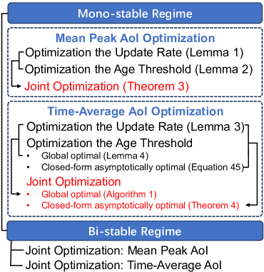
Figure 3: The logical flow in optimizing information freshness.

IV Mean Peak AoI Optimization

This section optimizes the mean peak AoI by adjusting the age threshold and update rate. The optimization problem can be formulated as

$$\begin{split}&\underset{\eta,A}{\min}\quad\hat{\Delta}_{0}\\ &~{}\mathrm{s.t.}\quad\eta\in(0,1],\\ &\quad~{}~{}~{}~{}~{}A\in\mathbb{N}.\end{split}$$ (24)

The age threshold is usually set as an integer, leading to a mixed integer programming problem in (24), which is non-trivial to solve. As such, we first convert the problem into a continuous one by relaxing the age threshold to a continuous variable and then round the result to an integer. More precisely, the relaxed optimization problem can be written as the following

$$\begin{split}&\underset{\eta,A}{\min}\quad\hat{\Delta}_{0}\\ &~{}\mathrm{s.t.}\quad\eta\in(0,1],\\ &\quad~{}~{}~{}~{}~{}A\in\mathbb{R^{+}}.\end{split}$$ (25)

This optimization problem can be decomposed into two subproblems: 1) optimizing the update rate $\eta$ given an age threshold $A$, and 2) optimizing the age threshold $A$ given an update rate $\eta$.

In the following, we will first investigate the solutions to these subproblems respectively to obtain a comprehensive understanding of the differences and similarities between the optimal parameters. Then, we solve (25) by jointly tuning the update rate and age threshold.

IV-A Optimizing the Update Rate

The following theorem presents the optimal update rate for a given age threshold.

Lemma 1.

Given an age threshold $A$, the optimal mean peak AoI $\hat{\Delta}_{0}^{\eta=\hat{\eta}^{*}_{A}}$ is given by

$$\hat{\Delta}_{0}^{\eta=\hat{\eta}^{*}_{|A}}=\begin{cases}\lambda cr^{2}\exp\left(1+\theta r^{\alpha}\rho^{-1}\right),&\text{if}~{}\lambda cr^{2}>1+Ap_{s,*}\\ A+\left(p_{\mathrm{s},*}\right)^{-1},&\text{otherwise}\end{cases}$$ (26)

which is achieved when the update rate $\eta$ is set to be

$$\hat{\eta}^{*}_{|A}=\begin{cases}\dfrac{1}{\lambda cr^{2}-A\exp\left(-1-\theta r^{\alpha}\rho^{-1}\right)},&\text{if}~{}\lambda cr^{2}>1+Ap_{s,*}\\ 1,&\text{otherwise}\end{cases}$$ (27)

where $p_{\mathrm{s},*}$ is the root of the following equation

$$p_{\mathrm{s},*}=\exp\left(-\frac{\lambda cr^{2}}{1+Ap_{\mathrm{s},*}}-\frac{\theta r^{\alpha}}{\rho}\right).$$ (28)

Proof:

Please see Appendix E. ∎

Lemma 1 shows that the optimal update rate shall be tuned to the maximum, i.e., $\hat{\eta}^{*}_{|A}=1$, when the $\lambda cr^{2}\leq 1+Ap_{\mathrm{s},*}$. This is because when the nodes are sparsely deployed, each receiver has a high chance of successfully receiving updates. As such, the AoI performance can be effectively improved by increasing update rates. In contrast, when the nodes are deployed densely, each source shall decrease its update rate to circumvent channel contention and promote timely information delivery across the network.

IV-B Optimizing the Age Threshold

The following theorem characterizes the optimal age threshold for a given update rate.

Lemma 2.

Given an update rate $\eta$, the optimal mean peak AoI $\hat{\Delta}_{0}^{A=\hat{A}^{*}_{\eta}}$ is given by

$$\hat{\Delta}_{0}^{A=\hat{A}^{*}_{|\eta}}=\begin{cases}\lambda cr^{2}\exp\left(1+\frac{\theta r^{\alpha}}{\rho}\right),&\text{if}~{}~{}\lambda cr^{2}>\dfrac{1}{\eta}\\ \frac{1}{\eta}\exp\left(\lambda cr^{2}\eta+\frac{\theta r^{\alpha}}{\rho}\right),&\text{otherwise}\end{cases}$$ (29)

which is achieved when the age threshold $A$ is set to be

$$\hat{A}^{*}_{|\eta}=\begin{cases}\left(\lambda cr^{2}-\dfrac{1}{\eta}\right)\exp\left(1+\dfrac{\theta r^{\alpha}}{\rho}\right),&\text{if}~{}~{}\lambda cr^{2}>\dfrac{1}{\eta}\\ 0,&\text{otherwise}.\end{cases}$$ (30)

Proof:

Please see Appendix F. ∎

Lemma 2 indicates that when the interference level is high, i.e., $\lambda cr^{2}\eta>1$, imposing an age threshold to the ALOHA-like protocol is beneficial for reducing mean peak AoI. Conversely, when the interference level is low, the conventional SA protocol is more preferable in decreasing the mean peak AoI.

IV-C Joint Optimization

By integrating results from the above, the theorem below presents a joint optimization of the update rate and age threshold that minimizes the mean peak AoI.

Theorem 3.

The optimal mean peak AoI is given by

$$\hat{\Delta}_{0}^{*}=\begin{cases}\lambda cr^{2}\exp\left(1+\theta r^{\alpha}\rho^{-1}\right),&\text{if}~{}~{}\lambda cr^{2}>1\\ \exp\left(\lambda cr^{2}+\theta r^{\alpha}\rho^{-1}\right),&\text{otherwise}\end{cases}$$ (31)

which is achieved when the age threshold and update rate together satisfy

$$(\hat{A}^{*},\hat{\eta}^{*})=\begin{cases}\left(A_{1},\eta_{1}\right),&\text{if}~{}~{}\lambda cr^{2}>1\\ \left(0,1\right),&\text{otherwise}\end{cases}$$ (32)

where $\left(A_{1},\eta_{1}\right)$ satisfied the following equation

$$A_{1}=\left(\lambda cr^{2}-\frac{1}{\eta_{1}}\right)\exp\left(1+\frac{\theta r^{\alpha}}{\rho}\right),$$ (33)

whereas $\eta_{1}$ shall be confined in the range $\eta_{1}\in\left[\frac{1}{\lambda cr^{2}},1\right]$.

Proof:

Please see Appendix G. ∎

From (33), we observe that the optimal age threshold increases with the optimal update rate to mitigate the induced interference. Moreover, when $\lambda cr^{2}\leq 1$, the optimal TSA configuration reduces to the conventional SA. In addition to these, a (perhaps) more important message conveyed by Theorem 3 is that by appropriately adjusting the update rate, SA can attain the same optimal mean peak AoI as TSA. In other words, TSA and SA are equivalent in minimizing the mean peak AoI.

Remark 3.

The optimal tuning of the update rate and the age threshold depends on the statistical traffic information (such as the spatial deployment density), instead of the real-time number of active nodes requesting transmission or prior experience. Such parameters are collected when the network is initially deployed.

V Time-Average AoI Optimization

This section presents the optimization of time-average AoI by solving the following optimization problem

$$\begin{split}&\underset{\eta,A}{\min}\quad\bar{\Delta}_{0}\\ &~{}\mathrm{s.t.}\quad\eta\in(0,1],\\ &\quad~{}~{}~{}~{}~{}A\in\mathbb{N}.\end{split}$$ (34)

Following similar approaches in the previous section, we relax the mixed integer programming problem (34) to a continuous one. Then, we decompose it into two subproblems and solve each one respectively. Finally, we integrate the whole procedure to establish a joint optimization. The concrete steps are detailed below.

V-A Optimizing the Update Rate

First, we optimize the update rate under a fixed age threshold, where the structural result is summarized as follows.

Lemma 3.

Given an age threshold $A$, the optimal time-average AoI $\bar{\Delta}_{0}^{\eta=\bar{\eta}^{*}_{|A}}$ can be achieved by setting the update rate as

$$\bar{\eta}^{*}_{|A}=\begin{cases}\dfrac{1}{\lambda cr^{2}-A\exp\left(-1-\theta r^{\alpha}\rho^{-1}\right)},&\text{if}~{}\lambda cr^{2}>1+Ap_{\mathrm{s},*};\\ 1,&\text{otherwise},\end{cases}$$ (35)

where $p_{s,*}$ is given by the solution to the following

$$p_{\mathrm{s},*}=\exp\left(-\frac{\lambda cr^{2}}{1+Ap_{\mathrm{s},*}}-\dfrac{\theta r^{\alpha}}{\rho}\right).$$ (36)

In this case, the time-average AoI is

$$\bar{\Delta}_{0}^{\eta=\bar{\eta}^{*}_{|A}}=\begin{cases}\dfrac{2\left(\lambda cr^{2}\exp\left(1+\theta r^{\alpha}\rho^{-1}\right)\right)^{2}+A(A+1)}{2\lambda cr^{2}\exp\left(1+\theta r^{\alpha}\rho^{-1}\right)}-A,\\ ~{}~{}~{}~{}~{}~{}~{}~{}~{}~{}~{}~{}~{}~{}~{}~{}~{}~{}~{}~{}~{}~{}~{}~{}~{}~{}~{}~{}~{}~{}~{}~{}~{}~{}~{}~{}~{}~{}~{}~{}\text{if}~{}\lambda cr^{2}>1+Ap_{\mathrm{s},*};\\ \\ \dfrac{A+1}{2}+\dfrac{A-1}{2(1+Ap_{\mathrm{s},*})}+\dfrac{1}{p_{\mathrm{s},*}(1+Ap_{\mathrm{s},*})},\\ ~{}~{}~{}~{}~{}~{}~{}~{}~{}~{}~{}~{}~{}~{}~{}~{}~{}~{}~{}~{}~{}~{}~{}~{}~{}~{}~{}~{}~{}~{}~{}~{}~{}~{}~{}~{}~{}~{}~{}~{}\text{otherwise}.\end{cases}$$ (37)

Proof:

Please see Appendix H. ∎

The condition that $\lambda cr^{2}\leq 1+Ap_{\mathrm{s},*}$ can be expressed as

$$p_{\mathrm{s},*}\geq\exp\left(-1-\theta r^{\alpha}\rho^{-1}\right).$$ (38)

This inequality indicates that if the transmission success probability is lower than $\exp\left(-1-\theta r^{\alpha}\rho^{-1}\right)$ when $\eta=1$, the update rate should be reduced to ensure the transmission success probability stabilizes at this value to optimize the time-average AoI. Because the age threshold always contributes to the transmission success probability, the optimal update rate goes up with the increase of the age threshold.

A comparison between (27) and (35) reveals that for a given age threshold, the optimal update rates that minimize the mean peak AoI and time-average AoI admit the same structure. This finding seems surprising, as the two performance metrics have very different analytical expressions (cf. Theorem 1). And the reason boils down to that, in essence, the core of optimizing the update rate for mean peak AoI and time-average AoI lies at maximizing the spatial throughput $\eta p_{\mathrm{s}}$.

V-B Optimizing the Age Threshold

In a similar vein, we explore the optimal structure of the age threshold under a fixed update rate. The following result provides a systematic approach to achieving this.

Lemma 4.

Given an update rate $\eta$, the optimal time-average AoI $\bar{\Delta}_{0}^{A=\bar{A}^{*}_{|\eta}}$ can be achieved by setting the age threshold as

$$\bar{A}^{*}_{|\eta}=\begin{cases}A_{1},&\text{if}~{}~{}\lambda cr^{2}>\frac{1}{\eta}\mathbb{W}_{0}\left(\frac{\eta}{2}\exp\left(-\frac{\theta r^{\alpha}}{\rho}\right)\right);\\ 0,&\text{otherwise},\end{cases}$$ (39)

where $\mathbb{W}_{0}(\cdot)$ is the principal branch of Lambert W function [34], and $A_{1}$ is the single non-zero root of the following equation

$$\begin{split}&\left(1+A_{1}\eta p_{\mathrm{s}}\right)\left(\eta\exp\left(\frac{-\lambda cr^{2}\eta}{1+A_{1}\eta p_{\mathrm{s}}}-\frac{\theta r^{\alpha}}{\rho}\right)-1\right)\\ &\quad\quad-\lambda cr^{2}\eta\left(1+A_{1}\eta p_{\mathrm{s}}\right)^{2}+\left(1+A_{1}\eta p_{\mathrm{s}}\right)^{3}=\lambda cr^{2}\eta.\end{split}$$ (40)

Proof:

Please see Appendix I. ∎

Remark 4.

The computational complexity (in terms of the number of iterations) in solving (40) can be reduced by first computing $(1+A_{1}\eta p_{\mathrm{s}})$ and then calculate $p_{\mathrm{s}}$, instead of directly solving (6) for the transmission success probability. The optimal age threshold $A_{1}$ can be obtained by combining the numerical evaluations of $(1+A_{1}\eta p_{\mathrm{s}})$ and $p_{\mathrm{s}}$.

According to Lemma 4, we note that the optimal age threshold is $\bar{A}^{*}_{|\eta}=0$ when

$$\lambda cr^{2}\leq\frac{1}{\eta}\mathbb{W}_{0}\left(\frac{\eta}{2}\exp\left(-\frac{\theta r^{\alpha}}{\rho}\right)\right),$$ (41)

indicating that when network interference is mild, one shall not impose any waiting duration at the source nodes but employ an SA-like protocol for the status updating. In contrast, TSA protocol is preferable when interference is severe, as it reduces concurrent transmissions, thus mitigating potential contentions. As a result, the nodes with urgent updating demands will benefit from a better transmission environment, which facilitates age performance.

The condition in (41) can be equivalently written as

$$\eta\leq\frac{-\ln\left(2\lambda cr^{2}\exp\left(\theta r^{\alpha}\rho^{-1}\right)\right)}{\lambda cr^{2}}.$$ (42)

This implies that TSA outperforms SA in terms of AoI when the update frequency is relatively high. Furthermore, when $\lambda cr^{2}>\tfrac{1}{2}\exp(-\theta r^{\alpha}\rho^{-1})$, TSA protocol consistently achieves a better time-average AoI than SA. Notably, these observations are in line with those drawn in [9], which are concluded based on a collision channel model.

While it is possible to solve equation (40) numerically, obtaining a closed-form solution (which could provide design insights) is challenging. In that respect, we leverage (tight) upper and lower bounds of the time-average AoI to facilitate our optimization. Specifically, we can derive a lower bound to the average AoI as

$$\bar{\Delta}^{\text{LB}}_{0}=\frac{A\eta p_{\mathrm{s}}+1}{2\eta p_{\mathrm{s}}}+\frac{1}{2\eta p_{\mathrm{s}}(1+A\eta p_{\mathrm{s}})},$$ (43)

and an upper bound as

$$\bar{\Delta}_{0}^{\text{UB}}=\frac{A\eta p_{\mathrm{s}}+1}{2\eta p_{\mathrm{s}}}+\frac{1}{2\eta p_{\mathrm{s}}(1+A\eta p_{\mathrm{s}})}+\frac{1}{2}.$$ (44)

Then, we take a derivative of $\bar{\Delta}^{\text{LB}}_{0}$ (and/or $\bar{\Delta}^{\text{UB}}_{0}$) with respect to $A$ and assign it to zero, which gives

$$(1\!+\!A\eta p_{\mathrm{s}})^{3}-\lambda cr^{2}\eta(1\!+\!A\eta p_{\mathrm{s}})^{2}-(1\!+\!A\eta p_{\mathrm{s}})-\lambda cr^{2}\eta=0.$$ (45)

By solving this equation, we obtain a closed-form expression for the suboptimal age threshold

$$\tilde{A}^{*}_{|\eta}=\frac{\Omega^{\frac{2}{3}}+(\lambda cr^{2}\eta-3)\Omega^{\frac{1}{3}}+(\lambda cr^{2}\eta)^{2}+3}{3\eta\Omega^{\frac{1}{3}}\exp\!\left(\dfrac{-3\lambda cr^{2}\eta\Omega^{\frac{1}{3}}}{\Omega^{\frac{2}{3}}\!+\!\lambda cr^{2}\eta\Omega^{\frac{1}{3}}\!+\!(\lambda cr^{2}\eta)^{2}\!+\!3}-\dfrac{\theta r^{\alpha}}{\rho}\right)},$$ (46)

where

$$\Omega=(\lambda cr^{2}\eta)^{3}+18\lambda cr^{2}\eta+3\sqrt{3}\sqrt{(\lambda cr^{2}\eta)^{4}+11(\lambda cr^{2}\eta)^{2}-1}.$$ (47)

Correspondingly, we have a closed-form expression, given in (48), for the time-average AoI under the suboptimal threshold. It is noteworthy that the difference between the bounds and the time-average AoI is at most $\frac{1}{2}-\frac{1}{2(1+A\eta p_{\mathrm{s}})}\in[0,\frac{1}{2})$, hence the suboptimal solution differs from the optimal one by (at most) a constant. Indeed, by comparing (16) and (44), we can see that the time-average AoI approaches the upper bound when the age threshold $A$ becomes large. Therefore, the solution given in (46) is asymptotically optimal.

Remark 5.

Comparing (30) and (46), we note that the optimal age threshold that minimizes the time-average AoI is larger than that for minimizing the mean peak AoI, owing to the necessity of reducing the variance in the status update intervals. This observation presents a marked distinction of TSA parameter configurations in optimizing different AoI metrics.

$$\bar{\Delta}_{0}^{A=\tilde{A}^{*}_{|\eta}}=\frac{\left(\Omega^{\frac{2}{3}}+\lambda cr^{2}\eta\Omega^{\frac{1}{3}}+(\lambda cr^{2}\eta)^{2}+3\right)^{2}\!\!+9\Omega^{\frac{2}{3}}\left(1-\eta\exp\left(\dfrac{-3\lambda cr^{2}\eta\Omega^{\frac{1}{3}}}{\Omega^{\frac{2}{3}}\!+\!\lambda cr^{2}\eta\Omega^{\frac{1}{3}}\!+\!(\lambda cr^{2}\eta)^{2}+3}-\dfrac{\theta r^{\alpha}}{\rho}\right)\right)}{6\eta\Omega^{\frac{1}{3}}\left(\Omega^{\frac{2}{3}}\!+\!\lambda cr^{2}\eta\Omega^{\frac{1}{3}}\!+\!(\lambda cr^{2}\eta)^{2}\!+\!3\right)\exp\left(\dfrac{-3\lambda cr^{2}\eta\Omega^{\frac{1}{3}}}{\Omega^{\frac{2}{3}}+\lambda cr^{2}\eta\Omega^{\frac{1}{3}}+(\lambda cr^{2}\eta)^{2}+3}-\dfrac{\theta r^{\alpha}}{\rho}\right)}+\frac{1}{2}.$$ (48)

 

V-C Joint Optimization

The previous subsections have explored the optimization of the update rate (resp. age threshold) given the age threshold (resp. update rate). This part will study how to jointly adjust the update rate and age threshold to further optimize the time-average AoI.

Algorithm 1 Iterative algorithm for AoI optimization

1:Input $\lambda$, $r$, $\theta$, $\rho$, $\alpha$, $n$, $\epsilon$

2:Initialize $i=1$ and choose $\bar{\eta}^{*}_{1}$ from (0,1] at random

3:repeat

4:***Optimize age threshold under a fixed update rate***

5:     if $\lambda cr^{2}\bar{\eta}^{*}_{i}>\mathbb{W}_{0}\left(\frac{\bar{\eta}^{*}_{i}}{2}\exp\left(-\theta r^{\alpha}\rho^{-1}\right)\right)$ then

6:         Use Bisection method to search for $\psi=1+\bar{A}^{*}_{i}\bar{\eta}^{*}_{i}p_{\mathrm{s}}$ from (40), with error accuracy $\epsilon$ and in the interval $[1,2e\lambda cr^{2}]$

7:         Compute $p_{\mathrm{s}}=\exp\left(-\lambda cr^{2}\psi^{-1}-\theta r^{\alpha}\rho^{-1}\right)$

8:         Compute $\bar{A}^{*}_{i}=(\psi-1)/{\bar{\eta}^{*}_{i}p_{\mathrm{s}}}$

9:         Compute $\bar{\Delta}_{0,i}$ based on $\bar{A}^{*}_{i}$, $\bar{\eta}^{*}_{i}$, $p_{\mathrm{s}}$, and (16)

10:     else

11:         Let $\bar{A}^{*}_{i}=0$

12:         Compute $\bar{\Delta}_{0,i}=\exp\left(\lambda cr^{2}\bar{\eta}^{*}_{i}+\theta r^{\alpha}\rho^{-1}\right)/\bar{\eta}^{*}_{i}$      

13:     $i\leftarrow i+1$

14:***Optimize update rate under a fixed age threshold***

15:     Compute $p_{\mathrm{s},*}$ base on $\eta=1$, $\bar{A}^{*}_{i-1}$, and (6)

16:     if $\lambda cr^{2}>1+\bar{A}^{*}_{i-1}p_{\mathrm{s},*}$ then

17:         Compute $\bar{\eta}^{*}_{i}$ based on $\bar{A}^{*}_{i-1}$, and (35)

18:         Compute $\bar{\Delta}_{0,i}$ based on $\bar{A}^{*}_{i-1}$, and (37)

19:     else

20:         Let $\bar{\eta}^{*}_{i}=1$

21:         Compute $\bar{\Delta}_{0,i}$ based on $\bar{A}^{*}_{i-1}$, and (37)      

22:until $|\bar{\Delta}_{0,i}-\bar{\Delta}_{0,i-1}|<\epsilon$

23:Assign $\bar{A}^{*}\leftarrow\bar{A}^{*}_{i-1}$, $\bar{\eta}^{*}\leftarrow\bar{\eta}^{*}_{i}$ and $\bar{\Delta}_{0}^{*}\leftarrow\bar{\Delta}_{0,i}$

24:return $\bar{A}^{*}$, $\bar{\eta}^{*}$, $\bar{\Delta}_{0}^{*}$

Since the age threshold and update rate have a composite influence on the time-average AoI (cf. (6) and (16)), it is challenging to characterize the optimal values of these factors explicitly. As such, based on Lemmas 3 and 4, we propose an iterative approach, presented in Algorithm 1, to jointly optimize the age threshold and update rate. Specifically, let $i$ denote the iteration index, while $\bar{\eta}^{*}_{i}$ and $\bar{A}^{*}_{i}$ represent the update rate and age threshold in the $i$th iteration, respectively. As detailed in Algorithm 1, we initialize $\bar{\eta}^{*}_{1}$ by randomly choosing a value from $(0,1]$, and then obtain $\bar{A}^{*}_{1}$ using Lemma 4. Based on $\bar{\eta}^{*}_{1}$ and Lemma 3, we further calculate $\bar{A}^{*}_{2}$ and $\bar{\eta}^{*}_{2}$. In each update of $\bar{\eta}_{i}^{*}$ and $\bar{A}^{*}_{i}$, we compute the corresponding time average AoI. The maximum iteration count is $n$. The iterations repeat until reaching the termination condition $|\bar{\Delta}_{0,i}-\bar{\Delta}_{0,i-1}|<\epsilon$, where $\epsilon$ is an error accuracy.

V-C1 Convergence and Optimality Analysis of the Proposed Algorithms

Upon dividing the problem (34), in Lemmas 3 and 4, we have demonstrated that each of the transformed sub-problems, i.e., (V.A) and (V.B), possess a unique optimal value. Consequently, obtaining the optimal solution for each sub-problem in the iterations enables the alternative iteration algorithm to converge to the global optimum.

V-C2 Complexity Analysis of the Proposed Algorithms

The sub-problem of fixing $\eta_{i}$ and computing $\bar{A}^{*}_{i}$ based on explicit expression (35) has a complexity of $O(1)$. The sub-problem of fixing $\bar{A}^{*}_{i-1}$ and computing $\bar{\eta}^{*}_{i}$ has demonstrated to have a unique optimal solution in Lemma 3. By utilizing bisection search and the method outlined in Remark 4, the complexity of this sub-problem is $O(\log_{2}\frac{2e\lambda cr^{2}}{\epsilon})$. The maximum iteration count is $n$. Consequently, the proposed algorithms have a computational complexity of $O(n\log_{2}\frac{2e\lambda cr^{2}}{\epsilon})$.

Furthermore, we can derive a structural form for the age threshold and update rate pair by leveraging the analytical expression in (48), which is asymptotically optimal.

Theorem 4.

The optimal time-average AoI $\bar{\Delta}_{0}^{*}$ is achieved when the age threshold and the update rate are jointly set as

$$\left(\bar{A}^{*},\bar{\eta}^{*}\right)=\begin{cases}(A_{*},1),&\text{if}~{}\lambda cr^{2}>\mathbb{W}_{0}\left(\frac{1}{2}\exp\left(-\frac{\theta r^{\alpha}}{\rho}\right)\right);\\ \left(0,1\right),&\text{otherwise},\end{cases}$$ (49)

where a closed-form approximation of $A_{*}$ is given by

$$A_{*}\approx\frac{\Omega_{*}^{\frac{2}{3}}+(\lambda cr^{2}-3)\Omega_{*}^{\frac{1}{3}}+(\lambda cr^{2})^{2}+3}{3\Omega_{*}^{\frac{1}{3}}\exp\left(\dfrac{-3\lambda cr^{2}\Omega_{*}^{\frac{1}{3}}}{\Omega_{*}^{\frac{2}{3}}+\lambda cr^{2}\Omega_{*}^{\frac{1}{3}}+(\lambda cr^{2})^{2}+3}-\dfrac{\theta r^{\alpha}}{\rho}\right)},$$ (50)

in which

$$\Omega_{*}=(\lambda cr^{2})^{3}+18\lambda cr^{2}+3\sqrt{3}\sqrt{(\lambda cr^{2})^{4}+11(\lambda cr^{2})^{2}-1}.$$ (51)

The corresponding time-average AoI is given by (52).

$$\bar{\Delta}_{0}^{*}=\begin{cases}\dfrac{\left(\Omega_{*}^{\frac{2}{3}}+\lambda cr^{2}\Omega_{*}^{\frac{1}{3}}+(\lambda cr^{2})^{2}+3\right)^{2}\!\!+9\Omega_{*}^{\frac{2}{3}}\left(1-\exp\left(\dfrac{-3\lambda cr^{2}\Omega_{*}^{\frac{1}{3}}}{\Omega_{*}^{\frac{2}{3}}\!+\!\lambda cr^{2}\Omega_{*}^{\frac{1}{3}}\!+\!(\lambda cr^{2})^{2}+3}-\dfrac{\theta r^{\alpha}}{\rho}\right)\right)}{6\Omega_{*}^{\frac{1}{3}}\left(\Omega_{*}^{\frac{2}{3}}\!+\!\lambda cr^{2}\Omega_{*}^{\frac{1}{3}}\!+\!(\lambda cr^{2})^{2}\!+\!3\right)\exp\left(\dfrac{-3\lambda cr^{2}\Omega_{*}^{\frac{1}{3}}}{\Omega_{*}^{\frac{2}{3}}+\lambda cr^{2}\Omega_{*}^{\frac{1}{3}}+(\lambda cr^{2})^{2}+3}-\dfrac{\theta r^{\alpha}}{\rho}\right)}+\dfrac{1}{2},&\text{if}~{}\lambda cr^{2}>\mathbb{W}_{0}\left(\frac{\exp\left(-\frac{\theta r^{\alpha}}{\rho}\right)}{2}\right),\\ \exp(\lambda cr^{2}+\theta r^{\alpha}\rho^{-1}),&\text{otherwise}.\end{cases}$$ (52)

 

Proof:

Please see Appendix J. ∎

We can observe from the above analysis that at the AoI-optimal operating region, the update rate of TSA always equals one while the age threshold varies in accordance with the interference level.

Theorem 4 also allows us to investigate the scaling property of AoI under TSA. More precisely, when we densify the infrastructure (i.e., let $\lambda\rightarrow\infty$), the network becomes interference-limited (namely, the thermal noise is negligible), and the AoI scales as follows.

Corollary 3.

The optimal time-average AoI under TSA protocol scales with the deployment density as

$$\lim_{\lambda cr^{2}\to\infty}\frac{\bar{\Delta}_{0}^{*,\mathrm{TSA}}}{\lambda cr^{2}}=\frac{e}{2},$$ (53)

in which the optimal age threshold ${A}^{*}$ satisfies

$$\lim_{\lambda cr^{2}\to\infty}\frac{\bar{A}^{*}}{\lambda cr^{2}}=e.$$ (54)

In contrast, the optimal time-average AoI under SA protocol scales as

$$\lim_{\lambda cr^{2}\to\infty}\frac{\bar{\Delta}_{0}^{*,\mathrm{SA}}}{\lambda cr^{2}}=e.$$ (55)

This corollary unveils that the optimal mean peak AoI and time-average AoI under TSA and SA both scale linearly with the interference level, but TSA can reduce the increasing rate of time-average AoI to half of that under conventional SA. Note that the results in Corollary 3 are obtained from the SINR model, and they coincide with the conclusions in [9] developed under the collision model.

VI AoI optimization with bi-stable Region

In the previous derivations, we concentrate on optimizing the TSA protocol while putting aside the root distribution of the fixed-point equation in (6). According to the discussions in Section III-B, if $\lambda cr^{2}\eta>4$, the solutions to (6) fall in the bi-stable region, i.e., the network can stabilize in two distinct states, typically a high-efficiency state (i.e., $p_{\mathrm{s}}^{H}$) and a low-efficiency state (i.e., $p_{\mathrm{s}}^{L}$), depending on the initial conditions and the dynamics of the system. This section aims to address such an issue.

First of all, we can assess the difference between the two candidate steady state $p_{\mathrm{s}}^{H}$ and $p_{\mathrm{s}}^{L}$ according to the region provided in Remark 1, by taking a ratio between them, as

$$\begin{split}\frac{p_{\mathrm{s}}^{H}}{p_{\mathrm{s}}^{L}}&>\tfrac{\exp\left(-\tfrac{\theta r^{\alpha}}{\rho}-\tfrac{1}{\frac{1}{2}+\sqrt{\frac{1}{4}-\frac{1}{\lambda cr^{2}\eta}}}\right)}{\exp\left(-\tfrac{\theta r^{\alpha}}{\rho}-\tfrac{1}{\frac{1}{2}-\sqrt{\frac{1}{4}-\frac{1}{\lambda cr^{2}\eta}}}\right)}\\ &=\exp\left(\sqrt{(\lambda cr^{2}\eta)^{2}-4\lambda cr^{2}\eta}\right).\end{split}$$ (56)

This inequality demonstrates that in the bi-stable region, if the steady-state point shifts from $p_{\mathrm{s}}^{H}$ to $p_{\mathrm{s}}^{L}$, the performance loss increases exponentially with product of the interference level and update rate, i.e., $\lambda cr^{2}\eta$, if the parameters are not properly tuned. For example, at $\lambda cr^{2}\eta=6$, the performance loss can be more than $30$ times.

In light of the above challenge, we propose parameter tuning strategies for both mean peak AoI and time-average AoI to enhance the robustness against the bi-stage region situation.

Fig. 4 illustrates an example of the mono-stable and bi-stable regions to facilitate explanations of the optimization process. It also highlights instances where the optimization results from previous discussions fall within these two regions.

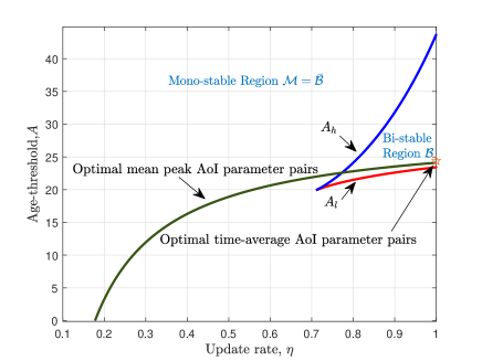
Figure 4: Bistable region $\mathcal{B}$ and monostable region $\mathcal{M}$.

VI-A Mean Peak AoI

For the mean peak AoI optimization, the optimal parameters pairs (33) intersect with the boundary line of the bi-stable region $A_{h}$. Then, the optimal parameter pairs are bisected by the curve $A_{h}$, with one portion lying in the mono-stable region and the other in the bi-stable region. Therefore, to achieve the optimal mean peak AoI, we only need to select optimal parameters pairs that fall within the mono-stable region. In short, the performance limits of mean peak AoI can be achieved even when the bi-stable region exists; only the tuning region for optimal parameter settings is limited.

The region of optimal update rate $\eta_{1}$ when optimal mean peak AoI is achieved in (33) can be expressed as

$$\eta_{1}\in\left[\frac{1}{\lambda cr^{2}},\min\left\{1,\frac{4.3509}{\lambda cr^{2}}\right\}\right].$$ (57)

The number $4.3509$ is the approximate value of $\lambda cr^{2}\eta$ when curve (33) intersects with $A_{h}$.

VI-B Time-Average AoI

For the time-average AoI optimization, the optimal performance is influenced by the bi-stable region, as the optimal operating point resides within it. Then, the suboptimal time-average AoI is achieved when $A=A_{h}$, which is given by

$$\min_{\eta\in\left[\frac{4}{\lambda cr^{2}},1\right]}~{}~{}\frac{A_{h}+1}{2}+\frac{1}{\eta p^{A=A_{h}}_{\mathrm{s}}}-\frac{A_{h}+1}{2\left(1+A_{h}\eta p^{A=A_{h}}_{\mathrm{s}}\right)}.$$ (58)

This outcome can be intuitively interpreted as follows:

First, due to the unstable nature of the bi-stable region, it’s imperative to fine-tune the network parameters to ensure that the system predominantly operates within the monostable region, avoiding the bi-stable region. Therefore, when the bi-stable region exists, the suboptimal parameters should possible to be choosed in the boundary between the mono-stable and bi-stable regions, i.e., $A_{l}$ or $A_{h}$ (the boundary line falls within the monostable region).

Then, based on Corollary 2, we can determine that, for a given update rate, the transmission success probability on the $A_{l}$ curve is lower than the undesired steady-state point within the bi-stable region, and also lower than that on the $A_{h}$, which characterizes an extremely adverse data transmission environment. Therefore, the suboptimal parameters shall be chosen on the boundary of $A_{h}$ rather than $A_{l}$.

Finally, upon investigating the time-average AoI performance along the boundary line $A_{h}$, we found that the time-average AoI decreases first and then increases as the update rate $\eta$ increases, which means the time-average AoI has a unique optimal value in the curve of $A_{h}$. Then, incorporating the following gradient information, i.e.,

$$\tfrac{\partial{\bar{\Delta}^{A=A_{h}}}}{\partial{\eta}}=\tfrac{1}{2}\tfrac{\partial{A_{h}}}{\partial{\eta}}\left(1-\tfrac{1-\eta p_{\mathrm{s}}^{A=A_{h}}}{\left(1+A_{h}\eta p_{\mathrm{s}}^{A=A_{h}}\right)^{2}}\right)$$ (59)

$$-\left(p_{\mathrm{s}}^{A=A_{h}}+\eta\tfrac{\partial{p_{\mathrm{s}}^{A=A_{h}}}}{\partial{\eta}}\right)\left(\tfrac{1}{\left(\eta p_{\mathrm{s}}^{A=A_{h}}\right)^{2}}-\tfrac{A_{h}(A_{h}+1)}{2\left(1+A_{h}\eta p_{\mathrm{s}}^{A=A_{h}}\right)^{2}}\right),$$

where the gradient $\frac{\partial{A_{h}}}{\partial{\eta}}$ and $\frac{\partial{p_{\mathrm{s}}^{A=A_{h}}}}{\partial{\eta}}$ are given as follows

$$\tfrac{\partial{A_{h}}}{\partial{\eta}}=\tfrac{1}{\eta^{2}}\exp{\left(\tfrac{1}{\tfrac{1}{2}-\sqrt{\tfrac{1}{4}-\tfrac{1}{\lambda cr^{2}\eta}}}\right)}\exp{\left(\theta r^{\alpha}\rho^{-1}\right)},$$ (60)

$$\tfrac{\partial{p_{\mathrm{s}}^{A=A_{h}}}}{\partial{\eta}}=\tfrac{\lambda cr^{2}p_{\mathrm{s}}^{A=A_{h}}}{\lambda cr^{2}A_{h}\eta^{2}p_{\mathrm{s}}^{A=A_{h}}-\left(1+A_{h}\eta p_{\mathrm{s}}^{A=A_{h}}\right)^{2}}$$ (61)

$$~{}\times\left(1-\exp\left(\tfrac{-\lambda cr^{2}\eta}{1+A_{h}\eta p_{\mathrm{s}}^{A=A_{h}}}\right)\exp{\left(\tfrac{1}{\tfrac{1}{2}-\sqrt{\tfrac{1}{4}-\tfrac{1}{\lambda cr^{2}\eta}}}\right)}\right),$$

the corresponding update rate in optimization problem (58) can be solved effectively by numerical method.

VII Numerical Results

In this section, we conduct simulations to verify the accuracy of the developed analysis and then use the numerical evaluations to explore the impact of different network parameters on the AoI performance. Specifically, at the beginning of each simulation run, the locations of source-destination pairs are scattered over a $100\times 100$ square area of unit size according to independent PPPs. We add the typical link to the network where the receiver is located at the center of the area. In each time slot, the locations of the links are rearranged independently according to the same PPPs except for the typical one. Each simulation lasts for $10^{6}$ time slots. We record the AoI statistics for each time slot of the typical link and then average them to obtain the mean peak and time-average AoI performance.

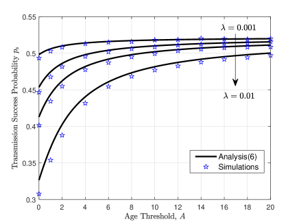
Figure 5: Transmission success probability $p_{\mathrm{s}}$ versus age threshold $A$. Update rate $\eta=1$, spatial deployment density $\lambda\in\{0.001,0.003,0.005,0.01\}$, decoding threshold $\theta=0~{}\text{dB}$, SNR $\rho=20~{}\text{dB}$, path-loss exponent $\alpha=3.8$ and transceiver distance $r=3$.

(a) $A=0$ and $A=10$.

Figure 6: AoI performance versus update rate under different age thresholds. Spatial deployment density $\lambda=0.02$, decoding threshold $\theta=0$ dB, SNR $\rho=20~{}\text{dB}$, path-loss exponent $\alpha=3.8$, and transceiver distance $r=4$.

(b) $A=20$ and $A=50$.

VII-A Transmission Success Probability

Fig. 5 plots the transmission success probability as a function of the age threshold under a variety of spatial deployment densities. We notice a close match between the analytical results and simulations, confirming our derivations in Theorem 1. Moreover, under the same configuration of other network parameters, the larger the spatial deployment density, the worse the transmission success probability due to the surging co-channel interference. On the other hand, the transmission success probability increases with the age threshold, demonstrating the effectiveness of the TSA protocol in interference mitigation. Furthermore, the gain becomes particularly significant when the spatial deployment density is large, revealing the potential of TSA protocol in elevating timeliness performance in dense networks.

VII-B Information Freshness versus Update Rate

Fig. 6 depicts the mean peak AoI and time-average AoI as functions of the update rate under different age thresholds. We can see from this figure that an optimal update rate exists that minimizes the mean peak AoI and time-average AoI, whereas the optimal value of the update rate is dependent on the age threshold. When the age threshold is relatively large, the optimal update rate also tends to be higher. This observation corroborates the interchangeable roles of both in mitigating channel contention.

Furthermore, we observe that the performance limits achieved by the TSA protocol in optimizing the mean peak AoI are equivalent to those achieved by the SA protocol, further substantiating this perspective. Yet, we also observe that integrating an age threshold into the SA protocol is beneficial for reducing time-average AoI, while such a threshold must be adjusted appropriately. This is attributed to the fact that, compared with adjusting the update rate, modifying the age threshold not only mitigates channel conflicts but also serves to equalize the intervals of update packet receptions. Consequently, it offers more pronounced gains for higher-order AoI metrics. Another noteworthy observation is that the optimal update rate (with a fixed age threshold) that realizes both the optimal mean peak AoI and the optimal time-average AoI is identical, whatever $\eta^{*}_{|A}<1$ in Fig. 6(a) or $\eta^{*}_{|A}=1$ in Fig. 6(b), corroborating the precision of our theoretical findings.

VII-C Information Freshness versus Age Threshold

Next, Fig. 7 plots the mean peak AoI and time-average AoI as functions of the age threshold under different spatial deployment densities. In this figure, the update rate is set to one (which is often optimal, according to Theorem 4). We can see that the solution given in (46) is almost indistinguishable from the optimality, confirming the accuracy of our analysis. Additionally, we note that the optimal age threshold increases with the spatial deployment density, owing to the more stringent requirement for interference management. Besides, the age threshold to achieve the optimal time-average AoI is higher than that for the optimal mean peak AoI because of the requirement for minimal fluctuations in the data update intervals.

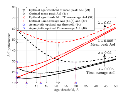
Figure 7: AoI performance versus age threshold under different deployment densities. Update rate $\eta=1$, decoding threshold $\theta=0.5$, SNR $\rho=20~{}\text{dB}$, path-loss exponent $\alpha=3.8$, and transceiver distance $r=5$.

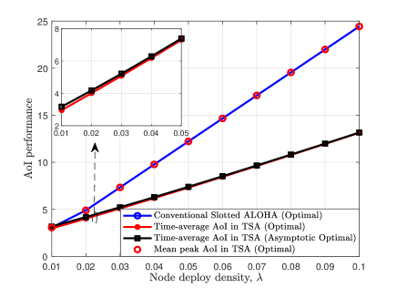
Figure 8: TSA performance gain. Decoding threshold $\theta=0$ dB, SNR $\rho=20~{}\text{dB}$, path-loss exponent $\alpha=3.8$, and transceiver distance $r=3$.

VII-D Scaling Law

Finally, Fig. 8 illustrates the performance gain of TSA over SA by drawing the optimal time-average AoI as a function of spatial deployment density. Specifically, at each value of $\lambda$, we calculate the optimal age threshold and update rate pair using Algorithm 1 and then compute the optimal time-average AoI. We also plot the results obtained from Theorem 4 in this figure. We can see that the optimal mean peak AoI and time-average AoI under SA and TSA increases almost linearly with the spatial deployment density, whilst the time-average AoI attained by TSA is approximately half of that under SA. This gain is mainly attributed to the advantage of TSA in ($a$) equalizing the status updating interval and ($b$) mitigating mutual interference, hence benefiting the AoI. Such observation also aligns with the theoretical analysis in Corollary 3. We also notice that the gap between the optimal AoI and that in Theorem 4 quickly diminishes, confirming the accuracy of our theoretical results.

VIII Conclusion

In this paper, we have developed an analytical framework to minimize AoI in random access networks by optimizing the TSA status updating protocol. We have derived analytical expressions for the transmission success probability, the mean peak AoI, and the time-average AoI of a typical link, accounting for effects from the update rate, age threshold, channel fading, and interference. Furthermore, we have obtained closed-form solutions for the optimal update rate (resp. age threshold) given a fixed age threshold (resp. update rate); we have also established a closed-form structure for the (almost) optimal update rate and age threshold pair. Our study showed that at the optimal operating point for time-average AoI, the update rate should be set to one while the age threshold varies according to the interference level. The optimization results have also revealed that under the same network configuration, the mean peak AoI and time-average AoI have an identical optimal update rate, yet the optimal threshold for time-average AoI is higher than that for mean peak AoI.

Furthemore, our analysis has identified the regime in which TSA outperforms SA in reducing AoI. Specifically, for the mean peak AoI, the TSA protocol exhibits comparable performance to the traditional slotted ALOHA protocol due to the interchangeable roles of tuning update rate and age threshold in mitigating channel contention. For the time-average AoI, TSA protocol outperforms SA due to its ability to equalize the intervals of update packet reception. The analysis has also disclosed the AoI scaling property, showing that the optimal mean peak AoI and time-average AoI under TSA and SA grow linearly with the deployment density; however, TSA can reduce the growth rate of time-average AoI to half of that under SA, thus, being efficient from an operation perspective.

It should be emphasized that while this study predominantly centers on the generate-at-will model, the proposed framework can also accommodate stochastic arrival patterns. Incorporating stochastic arrivals, exploring the intricate interplay among the age threshold, packet arrival, and channel access in TSA networks presents a compelling topic of discussion. Additionally, research has shown that the TSA protocol offers predictable gains for higher-order AoI metrics. However, the optimal operating point may not necessarily align perfectly with the metrics discussed in this paper. Therefore, utilizing the framework presented in this article to analyze and optimize other high-order AoI metrics with linear growth, as well as AoI metrics associated with nonlinear penalty functions, emerges as a significant direction for subsequent investigations. Moreover, enhancing the efficiency of IoT access in terms of operational costs, such as energy consumption and network lifetime, represents another promising avenue for investigation.

Appendix A Proof of Theorem 1

The transmission success probability can be derived as

$$\mathbb{P}(\text{SINR}_{0}>\theta)=\mathbb{P}\left(\frac{h_{00}r^{-\alpha}}{\sum_{i\neq 0}h_{i0}v_{i}||X_{i}||^{-\alpha}+\rho^{-1}}>\theta\right)$$

$$=\mathbb{P}\left(h_{00}>\theta r^{\alpha}\left(\sum_{i\neq 0}h_{i0}v_{i}||X_{i}||^{-\alpha}+\rho^{-1}\right)\right)$$

$$=\exp\left(-\theta r^{\alpha}\rho^{-1}\right)\prod_{i\neq 0}\exp\left(-\theta r^{\alpha}h_{i0}v_{i}||X_{i}||^{-\alpha}\right)$$

$$\overset{(a)}{=}\exp\left(-\theta r^{\alpha}\rho^{-1}\right)\prod_{i\neq 0}\left(\frac{1}{1+\theta r^{\alpha}v_{i}||X_{i}||^{-\alpha}}\right)$$

$$\overset{(b)}{\approx}e^{-\theta r^{\alpha}\rho^{-1}}\prod_{i\neq 0}\left(1-\eta\mathbb{P}(\Delta_{i}(t)>A)+\frac{\eta\mathbb{P}(\Delta_{i}(t)>A)}{1+\theta r^{\alpha}||X_{i}||^{-\alpha}}\right)$$

$$=e^{-\theta r^{\alpha}\rho^{-1}}\prod_{i\neq 0}\left(1-\frac{\eta\mathbb{P}(\Delta_{i}(t)>A))}{1+||X_{i}||^{\alpha}/\left(\theta r^{\alpha}\right)}\right),$$ (62)

where (a) follows since $h_{ij}$ are i.i.d. random variables satisfy $h_{ij}\sim\exp\left(1\right)$, (b) follows as $v_{i}$ are independent of each other, and $\mathbb{P}(v_{i}=1)=\eta\mathbb{P}(\Delta_{i}(t)>A)$. The probability that the AoI $\Delta_{i}(t)$ exceed threshold $A$ can be expressed as

$$\mathbb{P}(\Delta_{i}(t)>A)=\frac{\frac{1}{\eta p_{\mathrm{s},i}}}{A+\frac{1}{\eta p_{\mathrm{s},i}}}=\frac{1}{1+A\eta p_{\mathrm{s},i}},$$ (63)

With the mobility model, the correlation of the received SINR of each transmitter becomes i.i.d. Thus, we drop the $i$ index. The spatiotemproal interaction among the queues can be captured by a identification $p_{\mathrm{s}}$, which can be expressed as

$$p_{\mathrm{s}} =\mathbb{P}(\text{SINR}_{0}>\theta)$$

$$=e^{-\theta r^{\alpha}\rho^{-1}}\prod_{i\neq 0}\left(1-\frac{\frac{\eta}{1+A\eta p_{\mathrm{s}}}}{1+||X_{i}||^{\alpha}/(\theta r^{\alpha})}\right)$$

$$=e^{-\theta r^{\alpha}\rho^{-1}}\times$$

$$~{}~{}~{}\exp\left(-\lambda\int_{x\in\mathbb{R}^{2}}\left[1-\left(1-\frac{\frac{\eta}{1+A\eta p_{\mathrm{s}}}}{1+||X_{i}||^{\alpha}/(\theta r^{\alpha})}\right)\right]dx\right)$$

$$=e^{-\theta r^{\alpha}\rho^{-1}}\exp\left(-\frac{2\pi\lambda}{\alpha}\int_{0}^{\infty}\frac{\frac{\eta}{1+A\eta p_{\mathrm{s}}}}{1+u/\theta r^{\alpha}}u^{\frac{2}{\alpha}-1}du\right)$$

$$=\exp\left(-\frac{\lambda\pi\eta r^{2}\theta^{\frac{2}{\alpha}}\Gamma\left(1-\frac{2}{\alpha}\right)\Gamma\left(1+\frac{2}{\alpha}\right)}{1+A\eta p_{\mathrm{s}}}-\frac{\theta r^{\alpha}}{\rho}\right).$$ (64)

The transmission success probability $p_{\mathrm{s}}$ can then be expressed as (6) in Theorem 1.

Appendix B Root analysis of (6): Corollary 1

We begin by constructing the following auxiliary function

$$f(p_{\mathrm{s}})=-\ln p_{\mathrm{s}}-\frac{M}{N+p_{\mathrm{s}}}-K,$$ (65)

where $M=\frac{\lambda cr^{2}}{A}$, $N=\frac{1}{A\eta}$, and $K=\theta r^{b}\rho^{-1}$. It is evident that $f(p_{\mathrm{s}})=0$ is the equivalent transformation of the fixed-point equation (6), and can be employed to analyze the number of non-zero root for simplicity. Subsequently, we take a derivative of $f(p_{\mathrm{s}})$, that is

$$f^{{}^{\prime}}(p_{\mathrm{s}})=\frac{\phi(p_{\mathrm{s}})}{p_{\mathrm{s}}(N+p_{\mathrm{s}})^{2}}.$$ (66)

The numerator of $f^{{}^{\prime}}(p_{\mathrm{s}})$, i.e., $\phi(p_{\mathrm{s}})$ is a quadratic function, which can be expressed as

$$\phi(p_{\mathrm{s}})=-\left(p_{\mathrm{s}}+N-\frac{M}{2}\right)^{2}+\frac{M^{2}}{4}-MN.$$ (67)

The following lemma demonstrates that the number of non-zero roots of (66) is determined by the zero-points of roots of (67).

Lemma 5.

$f(p_{\mathrm{s}})$ exhibits three non-zero roots of $0<p_{\mathrm{s}}^{L}<p_{\mathrm{s}}^{M}<p_{\mathrm{s}}^{H}<1$, if and only if $\phi(p_{\mathrm{s}})=0$ has two non-zero roots $0<p^{{}^{\prime}}_{\mathrm{s},1}<p^{{}^{\prime}}_{\mathrm{s},2}<1$ with $f(p^{{}^{\prime}}_{\mathrm{s},1})<0$ and $f(p^{{}^{\prime}}_{\mathrm{s},2})>0$; in the cases where $f(p^{{}^{\prime}}_{\mathrm{s},1})=0$ or $f(p^{{}^{\prime}}_{\mathrm{s},2})=0$; $f(p_{\mathrm{s}})=0$ has two non-zero roots, otherwise, $f(p_{\mathrm{s}})=0$ will solely have one non-zero root $0<p_{\mathrm{s}}<1$.

Proof:

Due to the fact $\underset{p_{\mathrm{s}}\to 0}{\lim}f(p_{\mathrm{s}})>0$, $f(1)=-\frac{M}{N+1}-K<0$, $f(p_{\mathrm{s}})$ is a continuous function, according to the zero-point theorem, $f(p_{\mathrm{s}})$ possesses a non-zero root at least. Furthermore, the denominator of the function $f^{{}^{\prime}}(p_{\mathrm{s}})$ is greater than zero for $p_{\mathrm{s}}\in(0,1]$. Consequently, the number of non-zero roots of $\phi(p_{\mathrm{s}})=0$ for $p_{\mathrm{s}}\in(0,1]$ determines the number of non-zero roots of $f^{{}^{\prime}}(p_{\mathrm{s}})=0$ for $p_{\mathrm{s}}\in(0,1]$, and we will only consider the root of $\phi(p_{\mathrm{s}})$ in the following scenarios.

(1) Assume that $\phi(p_{\mathrm{s}})=0$ has no non-zero root when $p_{\mathrm{s}}\in(0,1]$, it follows that in this case $\phi(p_{\mathrm{s}})<0$ for $p_{\mathrm{s}}\in(0,1]$. Consequently, $f^{{}^{\prime}}(p_{\mathrm{s}})<0$ and $f(p_{\mathrm{s}})$ decreases monotonically when $p_{\mathrm{s}}\in(0,1]$, Hence, $f(p_{\mathrm{s}})$ has only one non-zero root in this scenario.

(2) Assume that $\phi(p_{\mathrm{s}})=0$ has one non-zero root $0<p_{\mathrm{s}}^{{}^{\prime}}\leq 1$, we have the following scenarios:

(2.a) If $\phi(p_{\mathrm{s}})=0$ has two roots when $p_{\mathrm{s}}\in\mathbb{R}$, and one of them in range $p_{\mathrm{s}}\in(0,1)$, we denote the root in $(0,1)$ as $p_{\mathrm{s}}^{{}^{\prime}}$. Consequently, when $p_{\mathrm{s}}\in(0,p_{\mathrm{s}}^{{}^{\prime}})$, $f(p_{\mathrm{s}})$ monotonically decrease and $p_{\mathrm{s}}\in(p_{\mathrm{s}}^{{}^{\prime}},1)$, $f(p_{\mathrm{s}})$ monotonically increase. Since we have $f(1)<0$, thus $f(p_{\mathrm{s}})$ only has one non-zero root.

(2.b) If $\phi(p_{\mathrm{s}})=0$ has one root when $p_{\mathrm{s}}\in\mathbb{R}$, and this root in range $p_{\mathrm{s}}\in(0,1)$, then $f(p_{\mathrm{s}})$ monotonically decrease when $p_{\mathrm{s}}\in(0,1)$, so $f(p_{\mathrm{s}})$ only has one non-zero root. Combining two cases, when $\phi(p_{\mathrm{s}})=0$ has one non-zero root, $f(p_{\mathrm{s}})=0$ only has one non-zero root.

Combining these two cases, when $\phi(p_{\mathrm{s}})=0$ has one non-zero root, $f(p_{\mathrm{s}})=0$ only has one non-zero root.

(3) Assume that $\phi(p_{\mathrm{s}})=0$ has two non-zero roots $0<p^{{}^{\prime}}_{\mathrm{s},1}<p^{{}^{\prime}}_{\mathrm{s},2}<1$, then we have

(3.a) If $p_{\mathrm{s},2}^{{}^{\prime}}=1$, then $\phi(p_{\mathrm{s}})<0$ for $p_{\mathrm{s}}\in(0,p_{\mathrm{s},1}^{{}^{\prime}})$ and $\phi(p_{\mathrm{s}})>0$ for $p_{\mathrm{s}}\in(p_{\mathrm{s},1}^{{}^{\prime}},1)$. Consequently, $f^{{}^{\prime}}(p_{\mathrm{s}})<0$ for $p_{\mathrm{s}}\in(0,p_{\mathrm{s},1}^{{}^{\prime}})$ and $f^{{}^{\prime}}(p_{\mathrm{s}})>0$ for $p_{\mathrm{s}}\in(p_{\mathrm{s},1}^{{}^{\prime}},1)$, indicating that $f(p_{\mathrm{s}})$ monotonically decreases for $p_{\mathrm{s}}\in(0,p_{\mathrm{s},1}^{{}^{\prime}})$, and increases for $p_{\mathrm{s}}\in(p_{\mathrm{s},1}^{{}^{\prime}},1]$. Since $f(1)<0$, we can conclude that in this case, $f(p_{\mathrm{s}})=0$ only one non-zero root $0<p_{\mathrm{s}}^{H}<1$.

(3.b) If $p^{{}^{\prime}}_{\mathrm{s},2}<1$, then $\phi(p_{\mathrm{s}})<0$ for $p_{\mathrm{s}}\in(0,p^{{}^{\prime}}_{\mathrm{s},1})\cup(p^{{}^{\prime}}_{\mathrm{s},2},1)$, and $\phi(p_{\mathrm{s}})>0$ for $p_{\mathrm{s}}\in(p^{{}^{\prime}}_{\mathrm{s},1},p^{{}^{\prime}}_{\mathrm{s},2})$. As a result, $f^{{}^{\prime}}(p_{\mathrm{s}})<0$ for $p_{\mathrm{s}}\in(0,p^{{}^{\prime}}_{\mathrm{s},1})\cup(p^{{}^{\prime}}_{\mathrm{s},2},1)$, and $f^{{}^{\prime}}(p_{\mathrm{s}})>0$ for $p_{\mathrm{s}}\in(p^{{}^{\prime}}_{\mathrm{s},1},p^{{}^{\prime}}_{\mathrm{s},2})$, indicating that $f(p_{\mathrm{s}})$ monotonically decreases for $p_{\mathrm{s}}\in(0,p^{{}^{\prime}}_{\mathrm{s},1})\cup(p^{{}^{\prime}}_{\mathrm{s},2},1)$, and increases for $p\in(p^{{}^{\prime}}_{1},p^{{}^{\prime}}_{2})$.Then, we have if $f(p_{\mathrm{s},1}^{{}^{\prime}})>0$ or $f(p_{\mathrm{s},2}^{{}^{\prime}})<0$, $f(p_{\mathrm{s}})=0$ has one root $0<p_{\mathrm{s}}^{H}\leq 1$; when $f(p^{{}^{\prime}}_{\mathrm{s},1})=0$ or $f(p^{{}^{\prime}}_{\mathrm{s},2})=0$; $f(p_{\mathrm{s}})=0$ has two non-zero roots; otherwise, $f(p_{\mathrm{s}})=0$ has three non-zero roots $0<p_{\mathrm{s}}^{L}<p_{\mathrm{s}}^{M}<p_{\mathrm{s}}^{H}\leq 1$ in which $f(p_{\mathrm{s},1}^{{}^{\prime}})<0$ and $f(p_{\mathrm{s},2}^{{}^{\prime}})>0$. ∎

Lemma 4 further concludes the specific condition for $\phi(p_{\mathrm{s}})=0$ has two non-zero roots $0<p^{{}^{\prime}}_{\mathrm{s},1}<p^{{}^{\prime}}_{\mathrm{s},2}<1$ with $f(p^{{}^{\prime}}_{\mathrm{s},1})<0$ and $f(p^{{}^{\prime}}_{\mathrm{s},2})>0$.

Lemma 6.

$\phi(p_{\mathrm{s}})=0$ has two non-zero roots $0<p^{{}^{\prime}}_{\mathrm{s},1}<p^{{}^{\prime}}_{\mathrm{s},2}<1$ with $f(p^{{}^{\prime}}_{\mathrm{s},1})<0$ and $f(p^{{}^{\prime}}_{\mathrm{s},2})>0$ if and only if $\lambda cr^{2}>\frac{4}{\eta}$, and $A_{l}<A<A_{h}$, where $A_{l}$ and $A_{h}$ are respectively given by

$$A_{l}=\frac{\lambda cr^{2}\left(\frac{1}{2}+\sqrt{\frac{1}{4}-\frac{1}{\lambda cr^{2}\eta}}\right)-\frac{1}{\eta}}{\exp\left(-\frac{\theta r^{\alpha}}{\rho}-\frac{1}{\frac{1}{2}+\sqrt{\frac{1}{4}-\frac{1}{\lambda cr^{2}\eta}}}\right)};$$ (68)

$$A_{h}=\frac{\lambda cr^{2}\left(\frac{1}{2}-\sqrt{\frac{1}{4}-\frac{1}{\lambda cr^{2}\eta}}\right)-\frac{1}{\eta}}{\exp\left(-\frac{\theta r^{\alpha}}{\rho}-\frac{1}{\frac{1}{2}-\sqrt{\frac{1}{4}-\frac{1}{\lambda cr^{2}\eta}}}\right)}.$$ (69)

Proof:

Considering the properties of quadratic function, $\phi(p_{\mathrm{s}})=0$ has two non-zero roots when $\underset{p_{\mathrm{s}}\to 0}{\lim}~{}\phi(p_{\mathrm{s}})<0$, $\underset{p_{\mathrm{s}}\to 1}{\lim}~{}\phi(p_{\mathrm{s}})<0$ and the peak value of $\phi(p_{\mathrm{s}})$ is larger than zero, that is:

$$~{}\underset{p_{\mathrm{s}}\to 0}{\lim}~{}\phi(p_{\mathrm{s}})=-N^{2}<0$$ (70)

$$~{}\underset{p_{\mathrm{s}}\to 1}{\lim}~{}\phi(p_{\mathrm{s}})=-\left(1+N-\frac{M}{2}\right)^{2}+\frac{M^{2}}{4}-MN<0$$ (71)

$$\underset{p_{\mathrm{s}}\in(0,1)}{\text{max}}~{}\phi(p_{\mathrm{s}})=\frac{M^{2}}{4}-MN>0$$ (72)

Combining (70), (71) and (72), we have

$$\frac{4}{\eta}<\lambda cr^{2}<\min\left\{A\left(\frac{1}{A\eta}+1\right)^{2},2A+\frac{2}{\eta}\right\}$$ (73)

For $\frac{4}{\eta}<\frac{2}{\eta}+2A$, we have $\frac{1}{A\eta^{2}}-A<0$ . Then,

$$A\left(\frac{1}{A\eta}+1\right)^{2}-\left(2A+\frac{2}{\eta}\right)=\frac{1}{A\eta^{2}}-A<0$$ (74)

which means (73) can be simplified as

$$\frac{4}{\eta}<\lambda cr^{2}<A\left(\frac{1}{A\eta}+1\right)^{2}$$ (75)

Then, we consider the condition that $f(p^{{}^{\prime}}_{\mathrm{s},1})<0$ and $f(p^{{}^{\prime}}_{\mathrm{s},2})>0$, i.e.,

$$f(p^{{}^{\prime}}_{\mathrm{s},1}) =-\frac{M}{\frac{{M}}{2}-\sqrt{\frac{{M}^{2}}{4}-MN}}-\ln\left(\frac{M}{2}-N-\sqrt{\frac{{M}^{2}}{4}-MN}\right)$$

$$-\theta r^{\alpha}\rho^{-1}<0,$$ (76)

and

$$f(p^{{}^{\prime}}_{\mathrm{s},2}) =-\frac{M}{\frac{M}{2}+\sqrt{\frac{{M}^{2}}{4}-MN}}-\ln\left(\frac{M}{2}-N+\sqrt{\frac{{M}^{2}}{4}-MN}\right)$$

$$-\theta r^{\alpha}\rho^{-1}>0,$$ (77)

By solving the inequalities (B) and (B), we then have

$$A>A_{l}=\frac{\lambda cr^{2}\left(\frac{1}{2}+\sqrt{\frac{1}{4}-\frac{1}{\lambda cr^{2}\eta}}\right)-\frac{1}{\eta}}{\exp\left(-\frac{\theta r^{\alpha}}{\rho}-\frac{1}{\frac{1}{2}+\sqrt{\frac{1}{4}-\frac{1}{\lambda cr^{2}\eta}}}\right)}$$ (78)

and

$$A<A_{h}=\frac{\lambda cr^{2}\left(\frac{1}{2}-\sqrt{\frac{1}{4}-\frac{1}{\lambda cr^{2}\eta}}\right)-\frac{1}{\eta}}{\exp\left(-\frac{\theta r^{\alpha}}{\rho}-\frac{1}{\frac{1}{2}-\sqrt{\frac{1}{4}-\frac{1}{\lambda cr^{2}\eta}}}\right)}.$$ (79)

Then, by solving the inequality $\lambda cR^{2}<A(\frac{1}{A\eta}+1)^{2}$, we have

$$A>\lambda cr^{2}\left(\frac{1}{2}+\sqrt{\frac{1}{4}-\frac{1}{\lambda cr^{2}\eta}}\right)-\frac{1}{\eta},$$ (80)

or

$$A<\lambda cr^{2}\left(\frac{1}{2}-\sqrt{\frac{1}{4}-\frac{1}{\lambda cr^{2}\eta}}\right)-\frac{1}{\eta}$$ (81)

When the condition $A_{l}<A<A_{h}$ is satisfied, the inequality (80) must be satisfied, and the inequality (81) will not be satisfied. Then, the condition (75) can be simplified as $\lambda cr^{2}>\frac{4}{\eta}$. ∎

Consequently, Corollary 1 can be proved by combining Lemma 5 and lemma 6.

Appendix C Proof of Monotony of $p^{L}_{\mathrm{s}}$ and $p^{H}_{\mathrm{s}}$: Corollary 2

By taking a partial derivative of $p_{\mathrm{s}}$ with respect to $A$, $\eta$, and $\lambda$, we have

$$\frac{\partial{p_{\mathrm{s}}}}{\partial{A}}=\frac{\lambda cr^{2}\eta^{2}p_{\mathrm{s}}^{2}}{(1+A\eta p_{\mathrm{s}})^{2}-\lambda cr^{2}A\eta^{2}p_{\mathrm{s}}}=\frac{-\lambda cr^{2}p_{\mathrm{s}}^{2}}{A^{2}}\frac{1}{\phi(p_{\mathrm{s}})};$$ (82)

$$\frac{\partial{p_{\mathrm{s}}}}{\partial{\eta}}=\frac{-\lambda cr^{2}p_{\mathrm{s}}}{(1+A\eta p_{\mathrm{s}})^{2}-\lambda cr^{2}A\eta^{2}p_{\mathrm{s}}}=\frac{\lambda cr^{2}p_{\mathrm{s}}}{A^{2}\eta^{2}}\frac{1}{\phi(p_{\mathrm{s}})};$$ (83)

$$\frac{\partial{p_{\mathrm{s}}}}{\partial{\lambda}}=\frac{-cr^{2}\eta p_{\mathrm{s}}(1+A\eta p_{\mathrm{s}})}{(1+A\eta p_{\mathrm{s}})^{2}-\lambda cr^{2}A\eta^{2}p_{\mathrm{s}}}=\frac{cr^{2}\eta p_{\mathrm{s}}(1+A\eta p_{\mathrm{s}})}{A^{2}\eta^{2}}\frac{1}{\phi(p_{\mathrm{s}})},$$ (84)

where $\phi(p_{\mathrm{s}})$ is consistence with equation (67). Then we prove $\phi(p_{\mathrm{s}}^{L})$ and $\phi(p_{\mathrm{s}}^{H})$ both smaller than zero.

• If $\phi(p_{\mathrm{s}})=0$ has no root for $p_{\mathrm{s}}\in(0,1]$, then $\phi(p_{\mathrm{s}})<0$ for $p_{\mathrm{s}}\in(0,1]$. In this case, (6) has one-zero root $p_{\mathrm{s}}^{H}$, and we have $\phi(p_{\mathrm{s}}^{H})<0$.

• If $\phi(p_{\mathrm{s}})=0$ has one root for $0<p^{{}^{\prime}}_{\mathrm{s},1}\leq 1$, we have:

  • If $\phi(p_{\mathrm{s}})=0$ has two roots when $p_{\mathrm{s}}\in\mathbb{R}$, and one of them in range $p_{\mathrm{s}}\in(0,1]$, then $\phi(p_{\mathrm{s}})<0$ for $p_{\mathrm{s}}\in(0,p^{{}^{\prime}}_{\mathrm{s},1})$ and $\phi(p_{\mathrm{s}})>0$ for $p_{\mathrm{s}}\in(p^{{}^{\prime}}_{\mathrm{s},1},1)$. The fixed point equation (6) has one-zero root $p_{\mathrm{s}}^{H}$, and $p_{\mathrm{s}}^{H}<p^{{}^{\prime}}_{\mathrm{s},1}$, we then have $\phi(p_{\mathrm{s}}^{H})<0$.

  • If $\phi(p_{\mathrm{s}})=0$ has one root when $p_{\mathrm{s}}\in\mathbb{R}$, and this root in range $p_{\mathrm{s}}\in(0,1)$, then $\phi(p_{\mathrm{s}})<0$ for $p_{\mathrm{s}}\in(0,1]$. (6) has one-zero root $\phi(p_{\mathrm{s}}^{H})$. We have $\phi(p_{\mathrm{s}}^{H})<0$.

• If $\phi(p_{\mathrm{s}})=0$ has two roots that $0<p^{{}^{\prime}}_{\mathrm{s},1}<p^{{}^{\prime}}_{\mathrm{s},2}<1$, two scenarios as follows:

  • If $p^{{}^{\prime}}_{\mathrm{s},2}=1$, then $\phi(p_{\mathrm{s}})<0$ for $p_{\mathrm{s}}\in(0,p^{{}^{\prime}}_{\mathrm{s},1})$ and $\phi(p_{\mathrm{s}})>0$ for $p_{\mathrm{s}}\in(p^{{}^{\prime}}_{\mathrm{s},1},1)$, (6) has one root $p_{\mathrm{s}}^{H}<p^{{}^{\prime}}_{\mathrm{s},1}$. We then have $\phi(p^{H}_{\mathrm{s}})<0$.

  • If $p^{{}^{\prime}}_{\mathrm{s},2}<1$, then $\phi(p_{\mathrm{s}})<0$ for $p_{\mathrm{s}}\in(0,p^{{}^{\prime}}_{\mathrm{s},1})\cup(p^{{}^{\prime}}_{\mathrm{s},2},1)$, and $\phi(p_{\mathrm{s}})>0$ for $p_{\mathrm{s}}\in(p^{{}^{\prime}}_{\mathrm{s},1},p^{{}^{\prime}}_{\mathrm{s},2})$. In this case, (6) may has one root $p_{\mathrm{s}}^{H}\in(0,p^{{}^{\prime}}_{\mathrm{s},1})\cup(p^{{}^{\prime}}_{\mathrm{s},2},1)$, or three roots $\phi(p_{\mathrm{s}}^{L})<p^{{}^{\prime}}_{\mathrm{s},1}<\phi(p_{\mathrm{s}}^{M})<p^{{}^{\prime}}_{\mathrm{s},2}<\phi(p_{\mathrm{s}}^{H})$. We then have $\phi(p_{\mathrm{s}}^{L})<0$ and $\phi(p_{\mathrm{s}}^{H})<0$.

In summary, $\phi(p_{\mathrm{s}}^{L})<0$ and $\phi(p_{\mathrm{s}}^{H})<0$ can be proved by combining above cases. Thus, it can be obtained from (82) – (84) that $\frac{\partial{p_{\mathrm{s}}}}{\partial{A}}>0$, $\frac{\partial{p_{\mathrm{s}}}}{\partial{\eta}}<0$ and $\frac{\partial{p_{\mathrm{s}}}}{\partial{\lambda}}<0$ at both the steady states $p_{\mathrm{s}}^{L}$ and $p_{\mathrm{s}}^{H}$. Therefore, the denominator of derivation satisfied the following inequality:

$$(1+A\eta p_{\mathrm{s}})^{2}-\lambda cr^{2}A\eta^{2}p_{\mathrm{s}}>0.$$ (85)

Appendix D AoI performance derivation: Theorem 2

Let us denote $I_{n}$ as the time interval between two consecutive transmission attempts over the typical link and $J_{k}$ the waiting time at the destination between successful receptions of the $k$-th and ($k+1$)-th updates, respectively. We have the following relationship between $I_{n}$ and $J_{k}$ according to the age threshold-based transmission protocol:

$$J_{k}=A+\sum_{n=1}^{N}I_{n}$$ (86)

where $N$ is a random variable that represents the number of attempts between two successful transmissions. We further introduce a variable $L_{k}$, which represents the area under the AoI evolution curve across the $k$-th successful update, as follows:

$$L_{k}=\sum_{j=1}^{J_{k}}j=\frac{1}{2}J_{k}(J_{k}+1).$$ (87)

Then, we can calculate the mean peak AoI and time average AoI over the typical link as:

$$\hat{\Delta}_{0}=\mathbb{E}[J_{k}],$$ (88)

and

$$\bar{\Delta}_{0}=\frac{\mathbb{E}[L_{k}]}{\mathbb{E}[J_{k}]}=\frac{1}{2}+\frac{\mathbb{E}[J_{k}^{2}]}{2\mathbb{E}[J_{k}]}.$$ (89)

Since the transmission success probability $p_{\mathrm{s}}$ is i.i.d over the time, we can compute $\mathbb{E}[J_{k}]$ and $\mathbb{E}[J_{k}^{2}]$ respectively as the following:

$$\mathbb{E}[J_{k}]=A+\sum_{n=1}^{\infty}\mathbb{E}[np_{\mathrm{s}}(1-p_{\mathrm{s}})^{n-1}]=A+\frac{\mathbb{E}[I_{n}]}{p_{\mathrm{s}}},$$ (90)

and

$$\begin{split}\mathbb{E}[J_{k}^{2}]&=A^{2}+2A\mathbb{E}\left[\sum_{n=1}^{N}I_{n}\right]+\mathbb{E}\left[\left(\sum_{n=1}^{N}I_{n}\right)^{2}\right]\\ &=A^{2}+\frac{2A\mathbb{E}[I_{n}]+\mathbb{E}[I_{n}^{2}]}{p_{\mathrm{s}}}+\frac{2(1-p_{\mathrm{s}})\left(\mathbb{E}[I_{n}]\right)^{2}}{p_{\mathrm{s}}^{2}}.\end{split}$$ (91)

when a source node is allowed to transmit, it generates new updates with probability $\eta$ independently over time, we have

$$\mathbb{E}[I_{n}]=\frac{1}{\eta},$$ (92)

$$\mathbb{E}[I_{n}^{2}]=\frac{2-\eta}{\eta^{2}}.$$ (93)

The age performance is derived by combining (88), (89), (90), (91), (92) and (93).

Appendix E Proof of lemma 1

By substituting (6) into (15), and take a partial derivative of $\hat{\Delta}_{0}$ with respect to $\eta$, we have

$$\frac{\partial{\hat{\Delta}_{0}}}{\partial{\eta}}=-\frac{1}{\eta^{2}p_{\mathrm{s}}}+\frac{\lambda cr^{2}}{\eta p_{\mathrm{s}}((1+A\eta p_{\mathrm{s}})^{2}-\lambda cr^{2}A\eta^{2}p_{\mathrm{s}})}.$$ (94)

At the two extreme operating points of $\eta$ (i.e., $\eta=0$ and $\eta=1$), we have

$$\lim_{\eta\to 0}\frac{\partial{\hat{\Delta}_{0}}}{\partial{\eta}}<0,$$ (95)

and

$$\lim_{\eta\to 1}\frac{\partial{\hat{\Delta}_{0}}}{\partial{\eta}}=-\frac{1}{p_{\mathrm{s}}}+\frac{\lambda cr^{2}}{(1+Ap_{\mathrm{s}})^{2}-\lambda cr^{2}Ap_{\mathrm{s}}}.$$ (96)

when $\lambda cr^{2}>1+Ap_{\mathrm{s},{*}}$, we have $\underset{{\eta\to 1}}{\lim}\frac{\partial{\hat{\Delta}_{0}}}{\partial{\eta}}>0$, the mean peak AoI can then be optimized when $\eta\in(0,1)$. By combining $\frac{\partial{\hat{\Delta}_{0}}}{\partial{\eta}}=0$ and (6), the optimal age threshold in mean peak AoI optimization can be obtained as

$$\hat{\eta}^{*}_{|A}=\dfrac{1}{\lambda cr^{2}-A\exp\left(-1-\theta r^{\alpha}\rho^{-1}\right)},$$ (97)

The optimal mean peak AoI can be obtained by substituting (107) into (15).

When $\lambda cr^{2}\leq 1+Ap_{\mathrm{s},{*}}$, on the other hand, the optimal age threshold is given by $\eta=1$, and the corresponding optimal mean peak AoI can be obtained by combining $\eta=1$ and (15).

Appendix F Proof of lemma 2

By substituting (6) into (15), and take a partial derivative of $\hat{\Delta}_{0}$ with respect to $A$, we have

$$\frac{\partial{\hat{\Delta}_{0}}}{\partial{A}}=1-\frac{\lambda cr^{2}\eta}{(1+A\eta p_{\mathrm{s}})^{2}-\lambda cr^{2}A\eta^{2}p_{\mathrm{s}}}.$$ (98)

At the two extreme operating points of $A$ (i.e., $A=0$ and $A\to\infty$), we have

$$\lim_{A\to 0}\frac{\partial{\hat{\Delta}_{0}}}{\partial{A}}=1-\lambda cr^{2}\eta,$$ (99)

and

$$\lim_{A\to\infty}\frac{\partial{\hat{\Delta}_{0}}}{\partial{A}}=1,$$ (100)

when $\lambda cr^{2}>\frac{1}{\eta}$, we have $\underset{{A\to 0}}{\lim}\frac{\partial{\hat{\Delta}_{0}}}{\partial{A}}<0$, the mean peak AoI can then be optimized when $A\in(0,\infty)$. By combining $\frac{\partial{\hat{\Delta}_{0}}}{\partial{A}}=0$ and (6), the optimal age threshold in mean peak AoI optimization can be obtained as

$$\hat{A}^{*}_{|\eta}=\left(\lambda cr^{2}-\dfrac{1}{\eta}\right)\exp\left(1+\theta r^{\alpha}\rho^{-1}\right).$$ (101)

The optimal mean peak AoI can be obtained by substituting (101) into (15).

On the other hand, when $\lambda cr^{2}\leq\frac{1}{\eta}$, the optimal age threshold is given by $A=0$, and the corresponding optimal mean peak AoI is obtained by combining $A=0$ and (15).

Appendix G Proof of Theorem 3

Combining equation (6), $\frac{\partial{\hat{\Delta}_{0}}}{\partial{\eta}}=0$ and $\frac{\partial{\hat{\Delta}_{0}}}{\partial{A}}=0$, we have

$$p_{\mathrm{s}}=\exp\left(-1-\theta r^{\alpha}\rho^{-1}\right).$$ (102)

Then, the optimal mean peak AoI can be achieved when $(\hat{A}^{*},\hat{\eta}^{*})$ satisfy

$$\hat{A}^{*}=\left(\lambda cr^{2}-\frac{1}{\hat{\eta}^{*}}\right)\exp\left(1+\theta r^{\alpha}\rho^{-1}\right).$$ (103)

Due to the fact $A\geq 0$, the optimal parameter pair $(A>0,\eta)$ exists when the condition $\lambda cr^{2}>\min\{\frac{1}{\eta}\}=1$ is satisfied; Otherwise, the optimal parameter setting is $(A=0,\eta=1)$. The corresponding optimal mean peak AoI can be obtained by substitute $(A,\eta)$ of above two situation in (15).

Appendix H Proof of Lemma 3

By substituting (6) into (16) and taking a partial derivative of $\bar{\Delta}_{0}$ with respect to $\eta$, we have

$$\frac{\partial{\bar{\Delta}_{0}}}{\partial{\eta}}=\left(p_{\mathrm{s}}-\frac{\lambda cr^{2}\eta p_{\mathrm{s}}}{\left(1+A\eta p_{\mathrm{s}}\right)^{2}-\lambda cr^{2}A\eta^{2}p_{\mathrm{s}}}\right)\left(\frac{A}{2(1+A\eta p_{\mathrm{s}})^{2}}-\frac{1}{\eta^{2}p_{\mathrm{s}}^{2}}\right).$$ (104)

At the two extreme operating points of $\eta$ (i.e., $\eta=0$ and $\eta=1$), we have $\underset{{\eta\to 0}}{\lim}\frac{\partial{\bar{\Delta}}}{\partial{\eta}}\to-\infty$, and

$$\lim_{\eta\to 1}\frac{\partial{\bar{\Delta}_{0}}}{\partial{\eta}}$$ (105)

$$=\left(p_{\mathrm{s},*}-\frac{\lambda cr^{2}p_{\mathrm{s},*}}{\left(1+Ap_{\mathrm{s},*}\right)^{2}-\lambda cr^{2}Ap_{\mathrm{s},*}}\right)\left(\frac{A}{2(1+Ap_{\mathrm{s},*})^{2}}-\frac{1}{p_{\mathrm{s},*}^{2}}\right).$$

We notice the last term of (105) satisfies

$$\frac{A}{2(1+Ap_{\mathrm{s},*})^{2}}-\frac{1}{(p_{\mathrm{s},*})^{2}}=\frac{Ap_{\mathrm{s},*}^{2}-2-4Ap_{\mathrm{s},*}-2A^{2}p_{\mathrm{s},*}^{2}}{2(1+Ap_{\mathrm{s},*})^{2}p_{\mathrm{s},*}^{2}}<0.$$ (106)

Therefore, if the first term of (105) is negative (this is achieved when $\lambda cr^{2}>1+Ap_{s,*}$), the time average AoI can be optimized by a specific $\eta\in(0,1)$. As such, by solving the equation $\frac{\partial{\bar{\Delta}_{0}}}{\partial{\eta}}=0$, the optimal update rate is obtained as:

$$\bar{\eta}^{*}_{|A}=\frac{1}{\lambda cr^{2}-A\exp\left(-1-\theta r^{\alpha}\rho^{-1}\right)}.$$ (107)

Then, the optimal time-average AoI follows by substituting (107) into (16). On the other hand, if $\lambda cr^{2}\leq 1+Ap_{s,*}$, the optimal update rate is achieved when $\eta=1$, and the optimal time-average AoI is obtained by combining $\eta=1$ and (16).

Appendix I Proof of Lemma 4

By substituting (6) into (16), and taking a partial derivative of $\bar{\Delta}_{0}$ with respect to $A$, we have

$$\begin{split}\frac{\partial{\bar{\Delta}_{0}}}{\partial{A}}&=\frac{A^{2}\eta^{2}p_{\mathrm{s}}^{2}+2A\eta p_{\mathrm{s}}+\eta p_{\mathrm{s}}}{2\left(1+A\eta p_{\mathrm{s}}\right)^{2}}\\ &-\frac{\lambda cr^{2}\eta\left(2+4A\eta p_{\mathrm{s}}+A^{2}\eta^{2}p_{\mathrm{s}}^{2}-A\eta^{2}p_{\mathrm{s}}^{2}\right)}{2\left(1+A\eta p_{\mathrm{s}}\right)^{2}\left(\left(1+A\eta p_{\mathrm{s}}\right)^{2}-\lambda cr^{2}A\eta^{2}p_{\mathrm{s}}\right)}.\end{split}$$ (108)

The two extreme operating points of the age threshold lead to $\underset{{A\to 0}}{\lim}\frac{\partial{\bar{\Delta}_{0}}}{\partial{A}}=\frac{1}{2}\eta p_{\mathrm{s}}^{A=0}-\lambda cr^{2}\eta$ and $\underset{A\to\infty}{\lim}\frac{\partial{\bar{\Delta}_{0}}}{\partial{A}}=\frac{1}{2}$, respectively.

When $\lambda cr^{2}\eta>\mathbb{W}_{0}\left(\frac{\eta}{2}\exp\left(-\theta r^{\alpha}\rho^{-1}\right)\right)$, we have $\underset{{A\to 0}}{\lim}\frac{\partial{\bar{\Delta}_{0}}}{\partial{A}}<0$. Since $\frac{\partial{\bar{\Delta}_{0}}}{\partial{A}}$ is continuous in $A$, Intermediate Value Theorem assures that $\frac{\partial{\bar{\Delta}_{0}}}{\partial{A}}=0$ has solutions in this case. As such, by combining $\frac{\partial{\bar{\Delta}_{0}}}{\partial{A}}=0$ and (6), the optimal age threshold can be obtained from solving the following equation

$$(1+A\eta p_{\mathrm{s}})^{3}-\lambda cr^{2}\eta(1+A\eta p_{\mathrm{s}})^{2}+(\eta p_{\mathrm{s}}-1)(1+A\eta p_{\mathrm{s}})-\lambda cr^{2}\eta=0.$$ (109)

(40) follows by combining (6) and (109).

The above analysis provides the conditions for the existence of roots. Next, we show that (40) (resp. (109)) has a unique non-zero root. We denote by $u=1+A\eta p_{\mathrm{s}}$ and introduce an auxiliary function as follows

$$\begin{split}&f(u)=u^{3}-\lambda cr^{2}\eta u^{2}\\ &\quad+\left(\eta\exp\left(\tfrac{\theta r^{\alpha}}{\rho}\right)\exp\left(-\tfrac{\lambda cr^{2}\eta}{u}\right)-1\right)u-\lambda cr^{2}\eta.\end{split}$$ (110)

Since $f(u)=0$ is equivalent to (40), it can be used to analyze the number of roots.

(1.1) When $\mathbb{W}_{0}\left(\frac{\eta}{2}\exp\left(-\theta r^{\alpha}\rho^{-1}\right)\right)<\lambda cr^{2}\eta\leq 1$, the first derivative of $f(u)$ can be expressed as follows:

$$\begin{split}&\frac{\partial{f(u)}}{\partial{u}}=3u^{2}-2\lambda cr^{2}\eta u-1\\ &\quad~{}~{}~{}~{}+\eta\exp\left(-\tfrac{\theta r^{\alpha}}{\rho}\right)\exp\left(-\tfrac{\lambda cr^{2}\eta}{u}\right)\left(1+\tfrac{\lambda cr^{2}\eta}{u}\right).\end{split}$$ (111)

Because $3u^{2}-2\lambda cr^{2}\eta u-1\geq 0$ for $u\geq 1$ and the last term of $\frac{\partial{f(u)}}{\partial{u}}$ is positive for $u\in[1,\infty)$. We have $\frac{\partial{f(u)}}{\partial{u}}>0$ for $u\in[1,\infty)$. Additionally, since $f(u)$ is monotonically increasing for $u\in[1,\infty)$, $f(u)=0$ has at most one root in this region.

(1.2) When $1<\lambda cr^{2}\eta\leq 3$, the second derivative of $f(u)$ satisfies

$$\begin{split}&\frac{\partial^{2}{f(u)}}{\partial{u^{2}}}=6u-2\lambda cr^{2}\eta\\ &\quad~{}~{}+\eta\exp\left(-\theta r^{\alpha}\rho^{-1}\right)\exp\left(-\tfrac{\lambda cr^{2}\eta}{u}\right)\tfrac{(\lambda cr^{2}\eta)^{2}}{u^{3}}>0.\end{split}$$ (112)

Therefore, the term $\frac{\partial f(u)}{\partial u}$ increases for $u\in[1,\infty)$. We denote by $v=\lambda cr^{2}\eta$ and let $g(v)=\underset{{u\in[1,\infty)}}{\min}\frac{\partial{f(u)}}{\partial{u}}=\frac{\partial{f(u)}}{\partial{u}}|_{u=1}$, which can be expressed as

$$\begin{split}&g(v)=2-2v+\eta\exp\left(-\theta r^{\alpha}\rho^{-1}\right)\exp\left(-v\right)(1+v).\end{split}$$ (113)

The first derivative of $g(v)$ satisfies $\frac{\partial g(v)}{\partial v}<0$, indicating that $g(v)$ decreases monotonically for $v=\lambda cr^{2}\eta\in(1,3)$. Additionally, notice that $g(1)>0$ and $g(3)<0$, $g(v)=0$ must have a root in $(1,3)$, which we denote by $\psi$. Consequently, if if $\lambda cr^{2}\in(1,\psi]$, $f(u)$ increases for $u\in(1,\infty)$; if $\lambda cr^{2}\in(\psi,3]$, $f(u)$ decreases first, and then increases with $u$. Moreover, since $f(1)<0$ and $\underset{u\to\infty}{\lim}f(u)>0$, $f(u)$ has a unique root in this case.

(1.3) When $\lambda cr^{2}\eta>3$, the third derivative of $f(u)$ satisfy

$$\begin{split}&\frac{\partial^{3}{f(u)}}{\partial{u^{3}}}=6+\eta\exp\left(-\theta r^{\alpha}\rho^{-1}\right)\times\\ &~{}~{}~{}~{}\exp\left(-\frac{\lambda cr^{2}\eta}{u}\right)\frac{(\lambda cr^{2}\eta)^{2}(\lambda cr^{2}\eta-3u)}{u^{5}}\\ &>6+\frac{(\lambda cr^{2}\eta)^{3}}{u^{3}}\exp\left(-\frac{\lambda cr^{2}\eta}{u}\right)\left(\frac{1-u}{u^{2}}\right)\\ &>6-\frac{(\lambda cr^{2}\eta)^{3}}{u^{3}}\exp\left(-\frac{\lambda cr^{2}\eta}{u}\right)>0.\end{split}$$ (114)

Then, the second derivative $\frac{\partial^{2}{f(u)}}{\partial{u^{2}}}$ increases for $u\in[1,\infty)$.

(a) If $\frac{\partial^{2}{f(u)}}{\partial{u^{2}}}|_{u=1}<0$, $\frac{\partial{f(u)}}{\partial{u}}$ decreases first, then increases for $u\in[1,\infty)$, and $\frac{\partial{f(u)}}{\partial{u}}|_{u=1}<0$, $\underset{u\to\infty}{\lim}\frac{\partial{f(u)}}{\partial{u}}>0$. Then, $f(u)$ decreases first and then increases versus $u$. Since $f(1)<0$ and $\underset{u\to\infty}{\lim}f(u)>0$, $f(u)$ has a root at most.

(b) If $\frac{\partial^{2}{f(u)}}{\partial{u^{2}}}|_{u=1}\geq 0$, $\frac{\partial{f(u)}}{\partial{u}}$ monotonically increases for $u\in[1,\infty)$, and $\frac{\partial{f(u)}}{\partial{u}}|_{u=1}<0$, $\underset{u\to\infty}{\lim}\frac{\partial{f(u)}}{\partial{u}}>0$. Then, $f(u)$ decreases first and then increases versus $u$. Since $f(1)<0$ and $\underset{u\to\infty}{\lim}f(u)>0$, $f(u)=0$ has a single root.

The discussions in (1.1), (1.2), and (1.3) confirm that (109) has a unique root, and the optimal age threshold $A_{1}$ is thus also unique. The results further indicate that when $\lambda cr^{2}\eta>\mathbb{W}_{0}\left(\frac{\eta}{2}\exp\left(-\theta r^{\alpha}\rho^{-1}\right)\right)$, $\bar{\Delta}_{0}$ decreases first, then increases with $A$, the solution of (40) is the global minimum.

When $\lambda cr^{2}\eta\leq\mathbb{W}_{0}\left(\frac{\eta}{2}\exp\left(-\theta r^{\alpha}\rho^{-1}\right)\right)$, $\bar{\Delta}_{0}$ monotonically increases for $A\in[0,+\infty)$. The optimal age threshold is thus given by $A=0$, and the corresponding optimal time-average AoI can be obtained by combining $A=0$ and (16).

Appendix J Proof of Theorem 4

We denote by $\bar{\Delta}_{0}^{*}=\underset{\{\eta\}}{\min}~{}\bar{\Delta}_{0}^{A=\tilde{A}^{*}_{|\eta}}$. On the one hand, for $\lambda cr^{2}\leq\frac{1}{\eta}\mathbb{W}_{0}\left(\frac{\eta}{2}\exp\left(-\frac{\theta r^{\alpha}}{\rho}\right)\right)$, we have

$$\bar{\Delta}_{0}^{A=A^{*}_{|\eta}}=\frac{1}{\eta}\exp\left(\lambda cr^{2}\eta+\theta r^{\alpha}\rho^{-1}\right).$$ (115)

Then, we take a derivative of $\bar{\Delta}_{0}^{A=A^{*}_{|\eta}}$ with respect to $\eta$, which gives

$$\tfrac{\partial{\bar{\Delta}_{0}^{A=A^{*}_{|\eta}}}}{\partial{\eta}}=\frac{\lambda cr^{2}\eta-1}{\eta^{2}}\exp\left(\lambda cr^{2}\eta+\theta r^{\alpha}\rho^{-1}\right).$$ (116)

Following this result, we note that if

$$\lambda cr^{2}<\frac{1}{\eta}\mathbb{W}_{0}\left(\frac{\eta}{2}\exp\left(-\frac{\theta r^{\alpha}}{\rho}\right)\right),$$ (117)

Due to the fact,

$$\frac{1}{\eta}\mathbb{W}_{0}\left(\frac{\eta}{2}\exp\left(-\frac{\theta r^{\alpha}}{\rho}\right)\right)<\frac{1}{\eta}\mathbb{W}_{0}\left(\frac{1}{2}\right)<\frac{1}{\eta},$$ (118)

there is $\frac{\partial{\bar{\Delta}_{0}^{A=A^{*}_{|\eta}}}}{\partial{\eta}}<0$, namely $\bar{\Delta}_{0}^{A=A^{*}_{|\eta}}$ decreases with the update rate $\eta$ in this region.

On the other hand, when $\lambda cr^{2}>\frac{1}{\eta}\mathbb{W}_{0}\left(\frac{\eta}{2}\exp\left(-\frac{\theta r^{\alpha}}{\rho}\right)\right)$, $\bar{\Delta}_{0}^{A=\bar{A}^{*}_{|\eta}}$ can be explicitly approximated by (48), and we have

$$\tfrac{\partial{\bar{\Delta}_{0}^{A=\tilde{A}^{*}_{|\eta}}}}{\partial{\eta}}=\tfrac{-3\left((\Omega^{\frac{1}{3}})^{{}^{\prime}}G(\eta)-\Omega^{\frac{1}{3}}G^{{}^{\prime}}(\eta)\right)}{2(G(\eta))^{2}}\\ -\tfrac{3\Omega^{\frac{1}{3}}\exp\left(\frac{3\lambda cr^{2}\eta\Omega^{\frac{1}{3}}}{G(\eta)}+\frac{\theta r^{\alpha}}{\rho}\right)}{\eta^{2}G(\eta)},$$ (119)

where $G(\eta)=\Omega^{\frac{2}{3}}+\lambda cr^{2}\eta\Omega^{\frac{1}{3}}+(\lambda cr^{2}\eta)^{2}+3$ and $\Omega$ is given in (47). Since the exponential term is greater than one, then

$$\dfrac{\partial{\bar{\Delta}_{0}^{A=\tilde{A}^{*}_{|\eta}}}}{\partial{\eta}}\leq-\frac{3\eta((\Omega^{\frac{1}{3}})^{{}^{\prime}}\eta G(\eta)-\Omega^{\frac{1}{3}}\eta G^{{}^{\prime}}(\eta))}{2\eta^{2}(G(\eta))^{2}}-\frac{6\eta\Omega^{\frac{1}{3}}G(\eta)}{2\eta^{2}(G(\eta))^{2}}$$

$$\quad~{}\overset{(a)}{=}\frac{3\left(G^{{}^{\prime}}(\eta)\eta\Omega^{\frac{1}{3}}-G(\eta)(\Omega^{\frac{1}{3}}+\eta(\Omega^{\frac{1}{3}})^{{}^{\prime}})\right)}{2\eta(G(\eta))^{2}}-\frac{3\Omega^{\frac{1}{3}}}{2\eta G(\eta)}\overset{(b)}{<}0,$$ (120)

where ($a$) follows algebraic manipulations. We further clarify the second inequality ($b$) in the following.

Since $G(\eta)$, $\Omega$, and $\eta$ are positive, we only need to show that $G^{{}^{\prime}}(\eta)\eta\Omega^{\frac{1}{3}}-G(\eta)(\Omega^{\frac{1}{3}}+\eta(\Omega^{\frac{1}{3}})^{{}^{\prime}})<0$. We expand this term as follows:

$$\begin{split}&G^{{}^{\prime}}(\eta)\eta\Omega^{\frac{1}{3}}-G(\eta)(\Omega^{\frac{1}{3}}+\eta(\Omega^{\frac{1}{3}})^{{}^{\prime}})=-\eta^{2}(\lambda cr^{2}-1)^{2}\Omega^{\frac{1}{3}}\\ &\quad\quad~{}~{}+\frac{\Omega^{{}^{\prime}}\eta}{3\Omega^{\frac{2}{3}}}\left(\Omega^{\frac{2}{3}}-(\lambda cr^{2}\eta)^{2}-3\right)-\Omega-(3-\eta^{2})\Omega^{\frac{1}{3}}.\end{split}$$ (121)

In (121), the sign of terms in the second line requires further clarification. The $\Omega^{{}^{\prime}}\eta$ in this term can be expressed as

$$\Omega^{{}^{\prime}}\eta=\Omega+2(\lambda cr^{2}\eta)^{3}+3\sqrt{3}\frac{(\lambda cr^{2}\eta)^{4}+1}{\sqrt{(\lambda cr^{2}\eta)^{4}+11(\lambda cr^{2}\eta)^{2}-1}},$$ (122)

which satisfy $\Omega^{{}^{\prime}}\eta<3\Omega$. Then, when $\Omega^{\frac{2}{3}}-(\lambda cr^{2}\eta)^{2}-3>0$, the terms in second line satisfy the following inequality

$$\begin{split}&\quad~{}~{}\frac{\Omega^{{}^{\prime}}\eta}{3\Omega^{\frac{2}{3}}}\left(\Omega^{\frac{2}{3}}-(\lambda cr^{2})^{2}\eta^{2}-3\right)-\Omega-(3-\eta^{2})(\Omega^{\frac{1}{3}})\\ &~{}<\Omega^{\frac{1}{3}}\left(\Omega^{\frac{2}{3}}-(\lambda cr^{2})^{2}\eta^{2}-3\right)-\Omega-(3-\eta^{2})(\Omega^{\frac{1}{3}})<0.\end{split}$$ (123)

Then, $G^{{}^{\prime}}(\eta)\eta\Omega^{\frac{1}{3}}-G(\eta)(\Omega^{\frac{1}{3}}+\eta(\Omega^{\frac{1}{3}})^{{}^{\prime}})<0$. On the other hand, when $\Omega^{\frac{2}{3}}-(\lambda cr^{2}\eta)^{2}-3<0$, due to $\Omega^{{}^{\prime}}\eta>0$, the condition $G^{{}^{\prime}}(\eta)\eta\Omega^{\frac{1}{3}}-G(\eta)(\Omega^{\frac{1}{3}}+\eta(\Omega^{\frac{1}{3}})^{{}^{\prime}})<0$ is still satisfied. Therefore, $\frac{\partial{\bar{\Delta}_{0}^{\tilde{A}^{*}_{|\eta}}}}{\partial{\eta}}<0$, which means that $\bar{\Delta}_{0}^{A=A^{*}_{|\eta}}$ decreases monotonically with update rate $\eta$ in this region.

Therefore, $\bar{\Delta}_{0}^{*}=\underset{\{\eta\}}{\min}~{}\bar{\Delta}_{0}^{A=\tilde{A}^{*}_{|\eta}}$ when $\eta=1$, and Theorem 4 can be obtained by combining Lemma 4, $\eta=1$ and (46).

References

• [1] N. Pappas, M. A. Abd-Elmagid, B. Zhou, W. Saad, and H. S. Dhillon, Age of Information: Foundations and Applications. Cambridge University Press, 2023.
• [2] R. D. Yates and S. K. Kaul, “The age of information: Real-time status updating by multiple sources,” IEEE Trans. Inf. Theory, vol. 65, no. 3, pp. 1807–1827, Sep. 2019.
• [3] R. D. Yates and S. K. Kaul, “Status updates over unreliable multiaccess channels,” in Proc. IEEE Int. Symp. Inf. Theory (ISIT), Aachen, Germany, pp. 331–335, Jun. 2017.
• [4] W. Zhan, D. Wu, X. Sun, Z. Guo, P. Liu, and J. Liu, “Peak age of information optimization of slotted Aloha: Fcfs versus lcfs,” IEEE Trans. Netw. Sci. Eng., pp. 1–13, May 2023.
• [5] B. Yu, Y. Cai, and D. Wu, “Joint access control and resource allocation for short-packet-based mmtc in status update systems,” IEEE J. Sel. Areas Commun., vol. 39, no. 3, pp. 851–865, Aug. 2021.
• [6] M. Salimnejad and N. Pappas, “On the age of information in a two-user multiple access setup,” Entropy, vol. 24, p. 542, 04 2022.
• [7] H. Chen, Y. Gu, and S. C. Liew, “Age-of-information dependent random access for massive IoT networks,” in proc. IEEE INFOCOM Workshop, Toronto, Canada, pp. 930–935, Jul. 2020.
• [8] O. T. Yavascan and E. Uysal, “Analysis of slotted ALOHA with an age threshold,” IEEE J. Sel. Areas Commun., vol. 39, no. 5, pp. 1456–1470, May 2021.
• [9] X. Chen, K. Gatsis, H. Hassani, and S. S. Bidokhti, “Age of information in random access channels,” IEEE Trans. Inf. Theory, vol. 68, no. 10, pp. 6548–6568, Jun. 2022.
• [10] J. Sun, Z. Jiang, B. Krishnamachari, S. Zhou, and Z. Niu, “Closed-form Whittle’s index-enabled random access for timely status update,” IEEE Trans. Commun., vol. 68, no. 3, pp. 1538–1551, Mar. 2020.
• [11] M. Ahmetoglu, O. T. Yavascan, and E. Uysal, “Mista: An age-optimized slotted ALOHA protocol,” IEEE Internet of Things J., vol. 9, no. 17, pp. 15484–15496, May 2022.
• [12] A. Munari, “Modern random access: An age of information perspective on irregular repetition slotted ALOHA,” IEEE Trans. Commun., vol. 69, no. 6, pp. 3572–3585, Feb. 2021.
• [13] J. Massey and P. Mathys, “The collision channel without feedback,” IEEE Trans. Inf. Theory, vol. 31, no. 2, pp. 192–204, Mar. 1985.
• [14] Y. Hu, Y. Zhong, and W. Zhang, “Age of information in Poisson networks,” in Proc. Int. Conf. Wireless Commun. Signal Process. (WCSP) Hangzhou, China, pp. 1–6, Oct. 2018.
• [15] P. D. Mankar, M. A. Abd-Elmagid, and H. S. Dhillon, “Spatial distribution of the mean peak age of information in wireless networks,” IEEE Trans. Wireless Commun., vol. 20, no. 7, pp. 4465–4479, Feb. 2021.
• [16] M. Emara, H. Elsawy, and G. Bauch, “A spatiotemporal model for peak AoI in uplink IoT networks: Time versus event-triggered traffic,” IEEE Internet of Things J., vol. 7, no. 8, pp. 6762–6777, Aug. 2020.
• [17] H. H. Yang, C. Xu, X. Wang, D. Feng, and T. Q. S. Quek, “Understanding age of information in large-scale wireless networks,” IEEE Trans. Wireless Commun., vol. 20, no. 5, pp. 3196–3210, May 2021.
• [18] H. H. Yang, A. Arafa, T. Q. S. Quek, and H. V. Poor, “Spatiotemporal analysis for age of information in random access networks under last-come first-serve with replacement protocol,” IEEE Trans. Wireless Commun., vol. 21, no. 4, pp. 2813–2829, Sep. 2022.
• [19] P. D. Mankar, Z. Chen, M. A. Abd-Elmagid, N. Pappas, and H. S. Dhillon, “Throughput and age of information in a cellular-based IoT network,” IEEE Trans. Wireless Commun., vol. 20, no. 12, pp. 8248–8263, Jun. 2021.
• [20] X. Sun, F. Zhao, H. H. Yang, W. Zhan, X. Wang, and T. Q. S. Quek, “Optimizing age of information in random-access Poisson networks,” IEEE Internet of Things J., vol. 9, no. 9, pp. 6816–6829, Sep. 2022.
• [21] F. Zhao, X. Sun, W. Zhan, X. Wang, and X. Chen, “Information freshness in random-access poisson network: Average AoI versus peak AoI,” in IEEE VTC2022-Fall, London, United Kingdom, pp. 1–6, Sep. 2022.
• [22] F. Zhao, X. Sun, W. Zhan, X. Wang, J. Gong, and X. Chen, “Age-energy tradeoff in random-access Poisson networks,” IEEE Trans. Green Commun. Netw., vol. 6, no. 4, pp. 2055–2072, Dec. 2022.
• [23] Z. Yue, H. H. Yang, M. Zhang, and N. Pappas, “Age of information under frame slotted ALOHA-based status updating protocol,” IEEE J. Sel. Areas Commun., vol. 41, no. 7, pp. 2071–2089, May 2023.
• [24] H. H. Yang, A. Arafa, T. Q. S. Quek, and H. V. Poor, “Optimizing information freshness in wireless networks: A stochastic geometry approach,” IEEE Trans. Mobile Comput., vol. 20, no. 6, pp. 2269–2280, Feb. 2021.
• [25] H. H. Yang, M. Song, C. Xu, X. Wang, and T. Q. S. Quek, “Locally adaptive status updating for optimizing age of information in Poisson networks,” IEEE Trans. Mobile Comput., pp. 1–13, Oct. 2022.
• [26] M. Song, H. H. Yang, H. Shan, J. Lee, and T. Q. S. Quek, “Age of information in wireless networks: Spatiotemporal analysis and locally adaptive power control,” IEEE Trans. Mobile Comput., vol. 22, no. 6, pp. 3123–3136, Dec. 2023.
• [27] H. H. Yang, N. Pappas, T. Q. Quek, and M. Haenggi, “Analysis of the age of information in age-threshold slotted ALOHA,” arXiv preprint arXiv:2306.09787, Jun. 2023.
• [28] F. Baccelli and B. Blaszczyszyn, Stochastic Geometry and Wireless Networks: Volume I Theory. Boston, MA, USA: Now Foundations and Trends, 2009.
• [29] M. Haenggi, Stochastic Geometry for Wireless Networks. Cambridge University Press, 2012.
• [30] K. Stamatiou and M. Haenggi, “Random-access Poisson networks: Stability and delay,” IEEE Commun. Lett., vol. 14, pp. 1035–1037, Nov. 2010.
• [31] M. Haenggi, “The meta distribution of the SIR in Poisson bipolar and cellular networks,” IEEE Trans. Wireless Commun., vol. 15, no. 4, pp. 2577–2589, Dec. 2016.
• [32] M. Haenggi, “The local delay in Poisson networks,” IEEE Trans. Inf. Theory, vol. 59, no. 3, pp. 1788–1802, Nov. 2013.
• [33] L. Dai, “Toward a coherent theory of CSMA and ALOHA,” IEEE Trans. Wireless Commun., vol. 12, no. 7, pp. 3428–3444, Jun. 2013.
• [34] R. M. Corless, G. H. Gonnet, D. E. G. Hare, D. J. Jeffrey and D. H. Knuth, “On the Lambert W function,” Adv. Comput. Math., vol. 5, pp. 329–359, Dec. 1996.