Country-Scale Cropland Mapping in Data-Scarce Settings Using Deep Learning: A Case Study of Nigeria

Abstract

Cropland maps are a core and critical component of remote-sensing-based agricultural monitoring. These maps can provide dense and up-to-date information about agricultural development without requiring regular field surveys, which are particularly challenging to execute in regions with limited accessibility. Machine learning is an effective tool for large-scale agricultural mapping, but relies on geo-referenced ground-truth data for model training and testing, which can be scarce or time-consuming to obtain. In this study, we explore the usefulness of combining a global cropland dataset and a hand-labeled dataset to train machine learning models for generating a new cropland map for Nigeria in 2020 at 10 m resolution. We provide the models with pixel-wise time series input data from remote sensing sources such as Sentinel-1 and 2, ERA5 climate data, and DEM data, in addition to binary labels indicating cropland presence. We manually labeled 1827 evenly distributed pixels across Nigeria, splitting them into 50% training, 25% validation, and 25% test sets used to fit the models and test our output map. We evaluate and compare the performance of single- and multi-headed Long Short-Term Memory (LSTM) neural network classifiers, a Random Forest classifier, and three existing 10 m resolution global land cover maps (Google’s Dynamic World, ESRI’s Land Cover, and ESA’s WorldCover) on our proposed test set. Given the regional variations in cropland appearance, we additionally experimented with excluding or sub-setting the global crowd-sourced Geowiki cropland dataset, to empirically assess the trade-off between data quantity and data quality in terms of the similarity to the target data distribution of Nigeria. We find that the existing WorldCover map performs the best with an F1-score of 0.825 and accuracy of 0.870 on the test set, followed by a single-headed LSTM model trained with our hand-labeled training samples and the Geowiki data points in Nigeria, with a F1-score of 0.814 and accuracy of 0.842. The code, data and output map generated with the best LSTM model are made available to the public to support research aiming to improve climate mitigation strategies, agricultural monitoring, and food security assessments.

Keywords Deep Learning, Agriculture, Satellite Images, Time Series, Transfer Learning, Large-scale mapping, Sentinel

1 Introduction

Agricultural maps are relevant for a variety of downstream applications ranging from policy making, early-warning systems for food security, and agricultural extension services [1]. The availability of free, granular, and high-cadence data from remote sensing sources like Sentinel-1 and 2 satellites has enabled the creation of detailed land cover and crop maps on a global scale [2]. Machine Learning (ML) is a widely employed methodology for generating these maps, given its capacity to process and extract useful information from large and diverse amounts of data, thereby aiding decision-making in agriculture [3].

Supervised machine learning, which requires high quality ground-truth data, has been applied extensively for generating crop maps all over the world [4, 5, 6]. Governments in High-Income Countries (HIC) regularly collect detailed information from farmers, including farm boundaries and crop types. This wealth of data has fueled research on generating accurate and high-resolution cropland, crop type and crop yield maps in regions like USA and Europe [4, 5, 7]. However, generating maps in countries where ground truth data is limited poses significant challenges. This data is time- and resource-consuming to collect, yet it is essential for validating the generated maps and for training the models to create them. As a mitigation strategy, one could attempt to leverage existing geo-referenced data related to cropland or crop type presence from other regions our countries to enhance the models performance. However, cropland data from different regions may present severe data distribution shifts associated with climate conditions, diverse agricultural practices, and the types of crops planted. Therefore, leveraging globally distributed data to generate agricultural maps in specific regions is not straight-forward and requires the use of different transfer learning strategies. Studies such as [6, 8] created cropland maps for Togo and Kenya leveraging global and local hand-labelled cropland samples by using a multi-task learning approach with an LSTM model. Other works have attempted to tackle the problem from a meta-learning approach [9, 10] or from a representation learning perspective using transformer models [11].

In this study, we focus on cropland mapping, framing it as a crop versus non-crop binary classification problem. We train ML models to provide a probability score of a given pixel being crop (positive class) given a multi-temporal array of pixel-wise data from different sensors (e.g. satellites images). Acquiring cropland ground-truth data, although a time-consuming endeavour that demands specialized expertise, can be achieved remotely by labeling high-resolution satellite or airborne image pixels through photo-interpretation [6]. Therefore, it is feasible to collect a minimal validation data set that allows for the creation and validation of cropland maps in new regions. In this work, we specifically aim to produce a cropland map for Nigeria using Sentinel data at a 10 m resolution for the year 2020, in order to support agricultural applications in the region. Nigeria stands as one of the leading food producers in Africa, with a population that accounts for about half of West-African population [12]. However, it currently lacks a cropland map at this level of spatial resolution. Given its significant agricultural importance for the region, we generate a small dataset of hand-labelled data for Nigeria to validate newly produced maps and to complement the training of different models to generate them. To this end, we investigate the usefulness of the global crowd-sourced Geowiki cropland dataset [13] together with our Nigeria dataset, by assessing and comparing an LSTM model and a Random Forest baseline. We provide the models with multi-temporal input data from Sentinel-1 and Sentinel-2 missions, complemented by local climate and topographic information (details in Section  2.1). For the LSTM, we explore standard and multi-task learning settings [6, 8]. Furthermore, we explore different dataset configurations such as sub-setting Geowiki to points within Nigeria or in neighbouring countries and compare our results to three 10 m resolution global land cover maps of the same year, which are briefly described in Section 3.2.

2 Data

2.1 Remote sensing data

Sentinel-1 and Sentinel-2 satellites from ESA’s Copernicus program provide data at ground sample distance (GSD) ranging from 10 to 60 m with frequent revisit time of 5 days world-wide, which is the best resolution freely available. Sentinel-2 captures multispectral data on bands ranging from visible and near-infrared (GSD of 10 m) to short-wave infrared (20 m to 60 m GSD), which are useful for vegetation monitoring and crop detection, by measuring how plants reflect different wavelengths [14]. On the other hand, Sentinel-1 contains a Synthetic Aperture Radar (SAR) sensor, which measures actively emitted radio wave signals in two polarization modes, as reflected by the surface. This data is useful for detecting traits related to surface roughness such as crop height, growth stage and soil moisture content [15]. We also include pixel-wise data of monthly total precipitation, monthly average temperature at 2 metres above the ground from ERA5 Climate Reanalysis Meteorological data [16], as well as elevation and slope derived from the Shuttle Radar Topography Mission’s (SRTM) Digital Elevation Model (DEM) [17].

The data was collected using the CropHarvest Python package [18] and Google Earth Engine [19] to produce a monthly per-pixel data array (i.e. each pixels is characterised by 12 values for each parameter considered) for a requested year. All Sentinel-2 bands are used and up-sampled to 10 m resolution except the B1 and B10, which have a coarse 60 m resolution and are predominantly meant for coastal aerosols and cirrus detection. Least-cloudy monthly composites of Sentinel-2 Level-1C images are obtained using an algorithm from [20]. Additionally, the Normalized Difference Vegetation Index (NDVI = $\frac{NIR-R}{NIR+R}$), derived from Sentinel-2 red (B4) and near-infrared (B8) bands, is also added given its value for assessing vegetation health and growth [21]. Thus, the output datasets contain modified Copernicus Sentinel data, ERA5, and SRTM data as processed by [18], yielding samples that are 18-dimensional arrays of features at 12 different monthly time steps, counting backwards from the respective label collection date. The 18 considered features are summarized on Table 1.

Table 1: Data features used in this study. All features were collected using the CropHarvest Python package [18].

Feature group	Feature descriptions	Feature count	Data Type	Source
Sentinel-1	VV polarization mode	1	Dynamic	Sentinel-1
	VH polarization mode	1	Dynamic	Sentinel-1
Sentinel-2	Visible bands (RGB)	3	Dynamic	Sentinel-2
	Visible and Near Infrared bands (VNIR)	5	Dynamic	Sentinel-2
	Short Wave Infrared bands (SWIR)	3	Dynamic	Sentinel-2
	NDVI	1	Dynamic	Sentinel-2
Climate	Monthly average precipitation	1	Dynamic	ERA5 [16]
	Monthly average temperature	1	Dynamic	ERA5 [16]
Topological	Elevation	1	Static	SRTM [17]
	Slope	1	Static	SRTM [17]

2.2 Cropland labels

These data refers to manually annotated ground-truth spatial coordinates indicating the presence (or absence) of visible cropland at a specific time. Each data point includes latitude and longitude coordinates, a reference date, and a label indicating whether it represents cropland (1) or non-cropland (0). These coordinates and the reference date are used to retrieve the corresponding remote sensing data.

2.2.1 Geowiki dataset

The Geowiki dataset consists of crowd-sourced points of cropland and non-cropland points sampled around the world [13]. The original dataset consists of roughly 36,000 points, each associated with a cropland probability score, which is the average of the labels provided by several human annotators. The Geowiki dataset is also readily available with the CropHavest package [18]. The data arrays cover September 2016 to September 2017, and match the labels’ collection date, to avoid mismatches due to possible land cover changes. The average label is transformed into 0 (non-cropland) or 1 (cropland) using a crop probability threshold of 0.5. In addition, we experiment with two subsets of this dataset: Geowiki Nigeria and Geowiki Neighbours. The number of points and class distribution for the full dataset and its subsets are described below:

• Geowiki World: contains all Geowiki dataset samples available in the CropHarvest package. The total number of collected samples are only 24761, presumably due to the input data availability, and out of which 13980 are labelled as cropland and 10781 labelled as non-cropland.

• Geowiki Nigeria: this subset includes all Geowiki samples available in the CropHarvest package that fall within Nigeria boundaries. They amount to 452 samples, out of which 312 are cropland and 140 are non-cropland samples.

• Geowiki Neighbours: this subset includes Geowiki Nigeria and all Geowiki samples available in the CropHarvest package that fall within the boundaries of the following countries close to Nigeria: Ghana, Togo, Benin, and Cameroon. This choice of countries was due to data availability and sharing of agro-ecological zones. Together they amount to 790 samples, from which 460 are cropland and 330 are non-cropland.

The Geowiki datasets described above are randomly split into 80 % training and 20 % validation data for the models.

2.2.2 Nigeria dataset

A dataset of evenly distributed points within Nigeria was generated and labelled as cropland or non-cropland via photo-interpretation. Spatial coordinates were randomly sampled within the country, until 2000 points spaced by least 15 km were obtained. Each point was examined using very high-resolution Google Satellite Imagery Basemap (which is mostly derived from Maxar’s 30 cm GSD mosaics) from 2020 in Google Earth Pro and labelled by an expert as cropland (1) or non-cropland (0) using QGIS. We consider cropland as arable land (cultivated or fallow) and areas where permanent (perennial) crops are grown, including orchards [22]. 1827 points were labelled and the remaining discarded as the class could not be determined by the human annotator from the available reference imagery. We note that given our constraint on the number of annotators and the remote labeling process, some labels may contain errors, particularly in regions affected by water scarcity, where distinguishing between fallow or wasteland was challenging. The dataset was then split into 50% train, 25% validation and 25% test sets using a stratified random sampling strategy, whereby each point within the validation and test sets were at least 30 km apart from each other. Using a stratified random splits covering the whole country is important to guarantee the quality of the output map at identifying cropland under the different climate and vegetation types found in the country, in a spatially homogeneous manner. The resulting splits are depicted in Figure 1. The coordinates of these points were used to query the respective pixel-wise data arrays from March 2019 - March 2020 using the CropHarvest package. The final dataset consists of 1822 data samples with a class distribution per split described in Table 2.

Table 2: Class distribution of Nigeria dataset. The cropland ratio refers to the proportion of points labelled as cropland in each data split.

Data split	Points	Cropland ratio
Train	913	0.417
Validation	454	0.399
Test	455	0.402
Total	1822	0.409

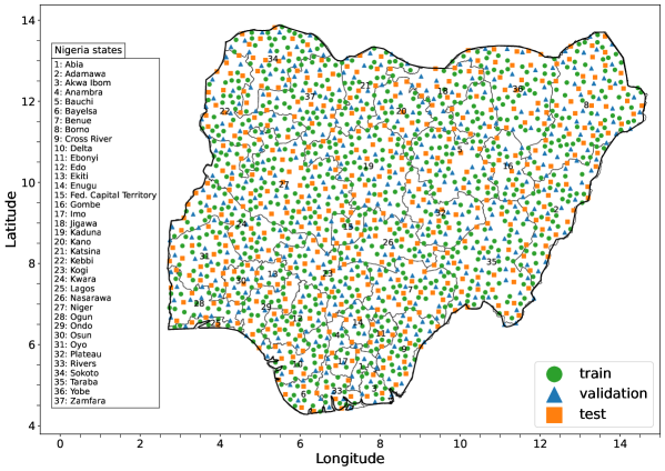
Figure 1: Geographical distribution of the 1827 points of the generated Nigeria dataset and its assigned splits for model training and evaluation. Nigeria state boundaries are taken from [23].

2.3 Dataset combination

We experiment with various combinations of the Geowiki dataset subsets, as described in Section 2.2.1, and considered both including and excluding the Nigeria dataset for training. To normalize the data, we initially calculated per-channel means and standard deviations independently using their training and validation samples. When merging datasets, as in [6], we combined all samples of the respective splits and calculated weighted per-channel means and standard deviations based on the number of samples in each dataset relative to the total combined samples. Subsequently, we applied this per-channel mean and standard deviation normalization to all samples in any data split.

3 Methods

3.1 Models

We followed [6, 8] and experimented with two LSTM neural network architectures: a standard one [24] and a multi-task (multi-head) implementation [6]. LSTM networks, which are a type of Recurrent Neural Network (RNN), excel in processing sequential data such as text or time series data. This makes them well-suited for crop classification tasks, as they can effectively capture temporal patterns and dependencies in remote sensing data [4]. The model is trained for binary classification of individual pixels. Each pixel in the input data is represented as a regularly sampled time series $\mathbf{X}=[\mathbf{x}_{1},\mathbf{x}_{2},...,\mathbf{x}_{12}]$ of 12 time steps of 18 dimensions each, i.e. $\mathbf{x}_{t}\in\mathbb{R}^{1\times 18}$. The model can have either one or two identical classification heads each consisting of a Multilayer Perceptron (MLP) and a sigmoid activation function to normalize the last activation between 0 and 1. This value can be interpreted as a posterior probability of cropland presence. When using the two classification heads, they both share the same LSTM backbone, but the global head classifies all the samples that are outside the boundaries of Nigeria and the local head classifies all samples that fall within Nigeria. This multi-headed architecture follows a multi-task learning approach [9]. In this setup, classifying global and local samples are treated as separate tasks handled by a dedicated head, but whereby they can leverage shared patterns learned by the LSTM backbone. The local head can then be used as a specialized classifier specialized for the region of interest.

This architecture is trained by minimizing the loss function of Eq. (1) [6], where $\mathcal{L}_{local}$ and $\mathcal{L}_{global}$ are Binary Cross-Entropy (BCE) loss functions of the local and global classification heads respectively. $\frac{W}{\alpha}$ is a weighting term, where $W$ is the proportion of global to local labels in each batch and $\alpha$ is a weighting hyper-parameter. This weighting term reduces the impact of the global head in the overall loss function and thus its influence over the parameters updates of the shared LSTM backbone, effectively giving more relevance to the local classification task in the overall architecture. When using only one head, all the samples are treated equally (no weighting).

For this work, both $\mathcal{L}_{local}$ and $\mathcal{L}_{global}$ BCE loss terms are additionally weighted according to the class distributions, as in Eq. (2), to better account for class imbalance. In here, $w^{(1)}$ and $w^{(0)}$ respectively represent the inverse of the cropland and non-cropland instances proportion from the total amount of local or global labels, $y$ is the label and $\hat{y}$ is the model prediction.

$$\mathcal{L}=\frac{W}{\alpha}\mathcal{L}_{global}+\mathcal{L}_{local}$$ (1)

$$\mathcal{L}_{i}=-(w^{(1)}\cdot y\cdot log(\hat{y})+w^{(0)}\cdot(1-y)\cdot log(1-\hat{y}))$$ (2)

All hyper-parameters were kept to default values from [6]. These include one hidden layer size of 64 units for the LSTM backbone, two classification layers on the MLPs, dropout of 0.2 between LSTM state updates and an $\alpha$ of 10. We trained all models using the Adam optimizer [25], with a learning rate of 0.001, and a batch size of 64, for a maximum of 100 epochs and early stopping with patience of 10 epochs on the validation set loss. A grid-search of {32, 64, 128} hidden units and {1, 2} LSTM hidden layers on the validation set confirmed that these are robust hyper-parameters for our datasets. We refer the reader to [6] for further details and a schematic diagram of the model architecture. The deep learning models are implemented in PyTorch [26]. We also included a Random Forest baseline model from scikit-learn [27] default implementation (100 trees with bootstrapping on the full dataset), due to its robustness and widespread use for crop and land cover classification [28].

3.2 Land cover maps

We additionally compare our models to three global land cover maps of 2020 at 10 m resolution. These maps are Google’s Dynamic World [29], ESRI’s 2020 Land Cover [30] and ESA’s WorldCover 2020 [31]. Dynamic World and ESRI Land Cover are two global land cover map produced with deep learning models, which were both trained using a dataset of 5 billion densely annotated patches of Sentinel-2 imagery distributed all over the world by experts and non-experts [2]. On the other hand, the global WorldCover map was produced with a Catboost model trained on pixels from 100 by 100 m patches of 141,000 locations around the world, which were labeled by experts [31, 2]. Both WorldCover and ESRI LandCover maps are produced yearly and have only discrete pixel assignments to classes, while Dynamic World is updated in near-real time (as new Sentinel-2 scenes become available approximately every 5 days) and also provides the probability for each pixel belonging to each of the possible classes. Another key difference is that WorldCover additionally uses Sentinel-1, together with Sentinel-2 and other auxiliary data, as well as being digitized with a smaller Minimum Mapping Distance (MMU) of 100 m², compared to 250 m² of the other two maps. While all maps are multi-class, we focus on the cropland class (named "crops" in ESRI and Dynamic World maps), and converted the maps to a binary version by assigning all non-cropland pixel values to the negative class and all cropland pixels to the positive class. This was done in order to be able to evaluate the maps performance on our Nigeria test set. We note that the cropland class in these maps do not consider tree plantations, which are categorized under a "trees" class for all three maps.

3.3 Evaluation metrics

We evaluated the models as well as the binarized land cover maps quantitatively by computing different performance metrics of their predictions on the Nigeria test set. The different metrics used are precision (proportion of correct predictions), recall (proportion of correctly identified samples or "probability of detection"), F1-score (harmonic mean between precision and recall and thus a symmetric measure of both), total accuracy (global proportion of correctly classified samples), and the Area Under the Receiver Operating Characteristic Curve (AUC ROC). These metrics are all typically used in classification settings and AUC ROC is exclusively used in binary classification for evaluating the ability of a classifier to correctly distinguish between the positive and negative classes. For all metrics a higher value is better, however since achieving a perfect recall and precision simultaneously is not possible in practice, a higher F1-score reflects a better trade-off between the two. The equations for precision, recall, F1-score and total accuracy are given in Eqs. (3), where TP, FP, FN, and TN are true positives, false positives, false negatives, and true negatives predictions, respectively. Note that for calculating the precision, recall, F1-score and total accuracy metrics, model prediction probabilities first need to be converted to binary predictions (0 or 1) by applying a threshold value. On the other hand, the AUC ROC score is calculated by computing the True Positive Rate ($\text{TPR}=\text{recall}$) and the False Positive Rate ($\text{FPR}=\frac{\text{FP}}{\text{FP+TN}}$, or "probability of false alarm") at different thresholds values to build the ROC and then calculating the area under this curve. The scikit-learn Python package was used for calculating all metrics [27].

$$\begin{aligned} \text{Precision}&=\frac{\text{TP}}{\text{TP}+\text{FP}}\\ \text{Recall}&=\frac{\text{TP}}{\text{TP}+\text{FN}}\\ \text{F1-score}&=\frac{2\times\text{Precision}\times\text{Recall}}{\text{Precision}+\text{Recall}}\\ \text{Total Accuracy}&=\frac{\text{TP + \text{TN}}}{\text{TP + FP + FN + TN}}\end{aligned}$$ (3)

In this study, a threshold of 0.5 was used as in [6], which is a sensible choice given there is no clear preference for a higher TPR or FPR in our cropland mapping use case (also note that this threshold is only required for model performance evaluation and is not used in any way during model training). Alternatively, this threshold could be optimized on a held-out validation set, or according to a desired confidence on model predictions, but we did not consider this setting.

4 Results

4.1 Main experiments

In this section we present the experimental results of the different models on the Nigeria test set, considering the different dataset configurations discussed in Section 2.3. We also compared our results to the global land cover maps introduced in Section 3.2 as benchmarks. The results are summarized on Table 3.

We can observe that the WorldCover map performs exceptionally well, particularly in terms of F1-score and total accuracy, compared to any of the models or other land cover maps. However, we also note that its recall is overall lower than those of the models, highlighting the need for careful consideration of the metric based on specific use cases. Among the implemented models, the single-headed LSTM model when using the Nigeria dataset and the Geowiki Nigeria subset achieves the best performance. Overall, all models show substantial improvement when the Nigeria dataset is included for training. It can also be observed that the Geowiki dataset is also beneficial in this case, but only when one of its subsets its used rather than the full Geowiki World dataset.

We can also observe that the best-performing Random Forest model is competitive to the best single-headed LSTM model and outperforms the multi-headed LSTM model. Nevertheless, the multi-headed LSTM model performs better than the Random Forest model when using the same Geowiki subset for training. Furthermore, the AUC ROC metric offer insights into model performance under different thresholds values, and we also depict the ROC curves for the two best models of each type (based on total accuracy) in Figure 2. In here, we can see how the Random Forest model performs better at lower thresholds (middle-right side of the curves), which can explain its higher AUC ROC scores compared to the other models.

Table 3: Results on the test set. A threshold of 0.5 was applied on the predicted probability to binarize into labels. Best results per metric are in bold and second best are underlined.

Map / Model	Geowiki dataset	Nigeria dataset	AUC ROC	Precision	Recall	F1-score	Accuracy
ESA WorldCover 2020	-	-	-	0.903	0.760	0.825	0.870
ESRI 2020	-	-	-	0.867	0.213	0.342	0.670
Dynamic World 2020	-	-	-	0.491	0.448	0.469	0.591
	$\times$	✓	0.911	0.774	0.787	0.780	0.822
	Nigeria	✓	0.915	0.782	0.825	0.803	0.837
	Neighbours	✓	0.916	0.791	0.765	0.778	0.824
Random Forest	World	✓	0.796	0.569	0.858	0.684	0.681
	Nigeria	$\times$	0.755	0.495	0.891	0.637	0.591
	Neighbours	$\times$	0.842	0.695	0.798	0.743	0.778
	World	$\times$	0.755	0.522	0.836	0.643	0.626
	$\times$	✓	0.908	0.772	0.776	0.774	0.818
	Nigeria	✓	0.907	0.771	0.863	0.814	0.842
	Neighbours	✓	0.906	0.788	0.831	0.809	0.842
Single-headed LSTM	World	✓	0.884	0.671	0.847	0.749	0.771
	Nigeria	$\times$	0.756	0.561	0.749	0.642	0.664
	Neighbours	$\times$	0.874	0.688	0.831	0.752	0.780
	World	$\times$	0.854	0.575	0.902	0.702	0.692
	Neighbours	✓	0.889	0.737	0.874	0.800	0.824
Multi-headed LSTM	World	✓	0.893	0.917	0.541	0.680	0.796
	Neighbours	$\times$	0.772	0.638	0.694	0.665	0.719
	World	$\times$	0.819	0.721	0.650	0.684	0.758

4.2 Ablation experiments

We conducted supplementary experiments by exclusively using the Sentinel-2 bands and by using only a regular BCE loss function for the LSTM models. The results for these experiments are presented on Table S1 and Table S2, respectively, in the Supplementary Material. Including additional data from Sentinel-1, climate and topography helps to significantly improve the results for all models under any dataset combination. However, it is interesting to note how the performance drop is most pronounced whenever Geowiki data is included, which might suggest that this additional features provide essential information for the models to identify the data distribution shifts. Furthermore, we also confirm that using a weighted BCE loss function improves the results from the single-headed LSTM models. However, its impact is particularly significant under dataset configurations that have a more pronounced class imbalance, such as when using the Geowiki Nigeria subset.

4.3 Nigeria cropland maps

We use our best model, the single-headed LSTM trained with the Geowiki Nigeria subset the Nigeria dataset, to generate both binary and probabilistic cropland maps covering the entire extent of Nigeria for the year 2020. The maps are presented on Figure 3. The cropland probability map offers additional valuable insights that are not available with the discrete WorldCover land cover map.

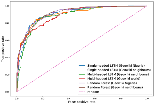
Figure 2: Receiving Operator Curve on the test set for two best models (regarding accuracy) of each type. All models represented here use the Nigeria hand-labelled data.

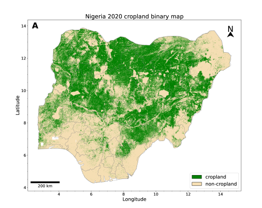
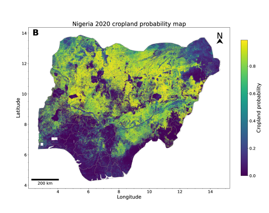
Figure 3: Binary (with a threshold of 0.5) and probability cropland maps for Nigeria in 2020 (A and B, respectively), generated with our the best model (single-headed LSTM model trained with Nigeria dataset and Geowiki Nigeria subset dataset). Figure 1 for the state names. Missing data within the country is shown in white.

5 Discussion

From our quantitative results we see that with the given remote sensing data and labels, the Random Forest and LSTM models do not achieve better performance on our cropland test set of Nigeria compared to the WorldCover land cover map. The three land cover maps evaluated also present drastic differences in performance. While WorldCover achieves an accuracy of 0.825 and F1-score of 0.870, both ESRI and Dynamic World maps lag several percentage points behind. In [2] a comparative analysis about these three maps was performed for all land cover classes and they suggest that WorldCover is better suited for resolving smaller and more complex agricultural landscapes. They argue this might be due to its lower MMU of 100 m² compared to 250 m² of the other two maps, and that it was likely trained for pixel-wise classification rather than for semantic segmentation. Therefore, this map may be specially well suited for detecting cropland in regions where smallholder farming is predominant, which also implies identifying isolated pixels representing small plots of cropland.

Among our assessed models, the best performing was the single-headed LSTM trained with the Geowiki Nigeria and Nigeria datasets, which achieved a total accuracy of 0.842 and an F1-score of 0.814, and was used for creating our Nigeria cropland maps. This performance is on pair with a Kenya cropland map (0.86 total accuracy and 0.84 F1-score) [8] and a Togo cropland map (0.83 total accuracy and 0.74 F1-score) [6], that were recently generated with a similar approach. Regarding the other models, we observe interesting results under the different combinations of datasets used for training. We learn that while including our local labels improves performance in all cases, it is also possible to train a good classifier using only labels from Geowiki, notably when using the Geowiki Neighbours subset. For this configuration, the single-headed LSTM model achieves a F1-score and accuracy greater than 0.75. Additionally, the multi-headed LSTM model is the only model where, when excluding the Nigeria dataset for training, using all of the Geowiki samples actually improves performance compared to using only a subset of Geowiki. This suggests that at least under certain cases, such as the absence of local labels for training, clever transfer learning techniques can indeed yield better results, compared to just combining all available data. The latter approach may in fact cause the resulting training data distribution to diverge significantly from that of the target country and dataset.

The advent of Sentinel satellite data has allowed for the creation of land cover, cropland and even crop yield maps at 10 m resolution, thus enabling the detection of smallholder farming and facilitating comprehensive agricultural monitoring at national scales [32]. In light of this progress, our study examines cropland mapping in Nigeria, comparing custom machine learning models trained for this task and recent global land cover maps at 10 m resolution. While we found that having enough local training data leads to improved results for custom models, the WorldCover land cover map is a robust choice for cropland mapping in Nigeria. Therefore, although there has been recent work in evaluating the accuracy of land cover maps for mapping agricultural land [33], there is a need for a systematic comparative assessment between these maps and those produced with custom, country-specific models for cropland classification such as those evaluated in this work. Further research could help practitioners and local governments to discern when relying on existing land cover maps suffices for their agricultural needs and when it is judicious to allocate resources for data collection and the development of croplands maps tailored to their specific requirements.

6 Conclusion

Up-to-date and accurate cropland maps provide fundamental information for many agricultural applications and are a critical tool for rapidly assessing the effects of climate change on food security at large-scales. In this work we developed two cropland maps for Nigeria in 2020 at 10 m resolution using deep learning and time series of remote sensing data. To this end, we created a dataset of uniformly-distributed points around the country and labelled them as cropland or non-cropland via photo-interpretation. We used this dataset for training and validation of a single- and multi-headed LSTM network and compared them to a random forest model and three global land cover maps. We investigated the benefit of combining our training data with different subsets of the Geowiki dataset, a large global dataset of cropland points. We found that the WorldCover land cover map has the best performance on our test set compared to all other maps and models. The best performing model was the single-headed LSTM model, obtained when combining our new training labels with the subset of points of the Geowiki dataset contained within Nigeria’s border. We observed that except in cases where the local manually labeled data were not provided to the model, using all of Geowiki labels is always detrimental for the model unless we use a dedicated transfer learning architecture such as a multi-headed LSTM classifier. However, we find that including training labels from Geowiki on countries close to the target country may complement and boost the performance of the model compared to using only labels from the country. Although collecting more training labels, either on-site or remotely, would generally lead to better results, the WorldCover land cover map proves to be a robust alternative for identifying cropland in Nigeria. This result is particularly relevant in cases where there is a lack of training labels available in the target region and insufficient resources for their collection. Nevertheless, land cover maps are generally static in time, whereas cropland maps can be generated by researchers or governments at any time, thus we consider that studying how to best leverage the available ground-truth data to be an important research topic for providing timely and accurate cropland extent information.

Data and code availability

The source code, as well as the links to download the data and output maps, are publicly available in the following repository: https://github.com/Joaquin-Gajardo/nigeria-crop-mask.

The maps can be visualized interactively with the following Google Earth Engine script (account needed): https://code.earthengine.google.com/df4bf4a222269289e982de7a48fb68fc

7 Supplementary Material

Table S1: Results comparison on the test set with only using Sentinel-2 bands and NDVI for training. A threshold of 0.5 was applied on the predicted probability to binarize into labels. Best results per metric are in bold and second best are underlined.

Model	Geowiki dataset	Nigeria dataset	AUC ROC	Precision	Recall	F1-score	Accuracy
	$\times$	✓	0.880	0.749	0.765	0.757	0.802
	Nigeria	✓	0.887	0.755	0.809	0.781	0.818
	Neighbours	✓	0.887	0.764	0.743	0.753	0.804
Random Forest	World	✓	0.722	0.587	0.667	0.624	0.677
	Nigeria	$\times$	0.606	0.471	0.574	0.517	0.569
	Neighbours	$\times$	0.778	0.723	0.470	0.570	0.714
	World	$\times$	0.691	0.530	0.732	0.615	0.631
	$\times$	✓	0.886	0.730	0.814	0.770	0.804
	Nigeria	✓	0.869	0.781	0.645	0.707	0.785
	Neighbours	✓	0.870	0.733	0.689	0.710	0.774
Single-headed LSTM	World	✓	0.750	0.584	0.683	0.630	0.677
	Nigeria	$\times$	0.658	0.667	0.284	0.398	0.655
	Neighbours	$\times$	0.810	0.681	0.607	0.642	0.727
	World	$\times$	0.804	0.608	0.863	0.713	0.721
	Neighbours	✓	0.884	0.810	0.650	0.721	0.798
Multi-headed LSTM	World	✓	0.847	0.780	0.601	0.679	0.771
	Neighbours	$\times$	0.808	0.702	0.475	0.567	0.708
	World	$\times$	0.600	0.600	0.050	0.091	0.604

Table S2: Results of LSTM model on test set without using a weighted BCE loss. A threshold of 0.5 was applied on the predicted probability to binarize into labels. Best results per metric are in bold and second best are underlined.

Model	Geowiki dataset	Nigeria dataset	AUC ROC	Precision	Recall	F1-score	Accuracy
	$\times$	✓	0.907	0.797	0.749	0.772	0.822
	Nigeria	✓	0.907	0.764	0.847	0.803	0.833
	Neighbours	✓	0.905	0.791	0.809	0.800	0.837
Single-headed LSTM	World	✓	0.868	0.704	0.792	0.746	0.782
	Nigeria	$\times$	0.785	0.497	0.874	0.633	0.593
	Neighbours	$\times$	0.872	0.632	0.918	0.748	0.752
	World	$\times$	0.846	0.538	0.929	0.681	0.651
	Neighbours	✓	0.890	0.743	0.869	0.801	0.826
Multi-headed LSTM	World	✓	0.892	0.920	0.437	0.593	0.758
	Neighbours	$\times$	0.827	0.591	0.831	0.691	0.701
	World	$\times$	0.814	0.723	0.628	0.673	0.754

References

- [1] Inbal Becker-Reshef, Brian Barker, Alyssa Whitcraft, Patricia Oliva, Kara Mobley, Christina Justice, and Ritvik Sahajpal. Crop Type Maps for Operational Global Agricultural Monitoring. Scientific Data, 10(1):172, March 2023.
- [2] Zander S. Venter, David N. Barton, Tirthankar Chakraborty, Trond Simensen, and Geethen Singh. Global 10 m land use land cover datasets: A comparison of dynamic world, world cover and esri land cover. Remote Sensing, 14(16), 2022.
- [3] Dashuai Wang, Wujing Cao, Fan Zhang, Zhuolin Li, Sheng Xu, and Xinyu Wu. A Review of Deep Learning in Multiscale Agricultural Sensing. Remote Sensing, 14(3):559, January 2022.
- [4] Marc RuBwurm and Marco Korner. Temporal Vegetation Modelling Using Long Short-Term Memory Networks for Crop Identification from Medium-Resolution Multi-spectral Satellite Images. In 2017 IEEE Conference on Computer Vision and Pattern Recognition Workshops (CVPRW), pages 1496–1504, Honolulu, HI, USA, July 2017. IEEE.
- [5] Mehmet Ozgur Turkoglu, Stefano D’Aronco, Gregor Perich, Frank Liebisch, Constantin Streit, Konrad Schindler, and Jan Dirk Wegner. Crop mapping from image time series: Deep learning with multi-scale label hierarchies. Remote Sensing of Environment, 264:112603, October 2021.
- [6] Hannah Kerner, Gabriel Tseng, Inbal Becker-Reshef, Catherine Nakalembe, Brian Barker, Blake Munshell, Madhava Paliyam, and Mehdi Hosseini. Rapid response crop maps in data sparse regions, 2020.
- [7] Gregor Perich, Mehmet Ozgur Turkoglu, Lukas Valentin Graf, Jan Dirk Wegner, Helge Aasen, Achim Walter, and Frank Liebisch. Pixel-based yield mapping and prediction from sentinel-2 using spectral indices and neural networks. Field Crops Research, 292:108824, 2023.
- [8] Tseng, Gabriel, Kerner, Hannah, Nakalembe, Catherine, and Becker-Reshef, Inbal. Annual and in-season mapping of cropland at field scale with sparse labels, November 2020. Type: dataset.
- [9] Gabriel Tseng, Hannah Kerner, Catherine Nakalembe, and Inbal Becker-Reshef. Learning to predict crop type from heterogeneous sparse labels using meta-learning. In 2021 IEEE/CVF Conference on Computer Vision and Pattern Recognition Workshops (CVPRW), pages 1111–1120, Nashville, TN, USA, June 2021. IEEE.
- [10] Gabriel Tseng, Hannah Kerner, and David Rolnick. Timl: Task-informed meta-learning for agriculture, 2022.
- [11] Gabriel Tseng, Ivan Zvonkov, Mirali Purohit, David Rolnick, and Hannah Kerner. Lightweight, pre-trained transformers for remote sensing timeseries, 2023.
- [12] Daniel Onwude, Thomas Motmans, Kanaha Shoji, Roberta Evangelista, Joaquin Gajardo, Divinefavor Odion, Nnaemeka Ikegwuonu, Olubayo Adekanmbi, Soufiane Hourri, and Thijs Defraeye. Bottlenecks in nigeria’s fresh food supply chain: What is the way forward? Trends in Food Science & Technology, 137:55–62, 2023.
- [13] Juan Carlos Laso Bayas, Myroslava Lesiv, François Waldner, Anne Schucknecht, Martina Duerauer, Linda See, Steffen Fritz, Dilek Fraisl, Inian Moorthy, Ian McCallum, Christoph Perger, Olha Danylo, Pierre Defourny, Javier Gallego, Sven Gilliams, Ibrar ul Hassan Akhtar, Swarup Jyoti Baishya, Mrinal Baruah, Khangsembou Bungnamei, Alfredo Campos, Trishna Changkakati, Anna Cipriani, Krishna Das, Keemee Das, Inamani Das, Kyle Frankel Davis, Purabi Hazarika, Brian Alan Johnson, Ziga Malek, Monia Elisa Molinari, Kripal Panging, Chandra Kant Pawe, Ana Pérez-Hoyos, Parag Kumar Sahariah, Dhrubajyoti Sahariah, Anup Saikia, Meghna Saikia, Peter Schlesinger, Elena Seidacaru, Kuleswar Singha, and John W Wilson. A global reference database of crowdsourced cropland data collected using the Geo-Wiki platform. Scientific Data, 4(1):170136, September 2017.
- [14] Francesco Vuolo, Martin Neuwirth, Markus Immitzer, Clement Atzberger, and Wai-Tim Ng. How much does multi-temporal sentinel-2 data improve crop type classification? International Journal of Applied Earth Observation and Geoinformation, 72:122–130, 2018.
- [15] Zheng Sun, Di Wang, and Geji Zhong. A review of crop classification using satellite-based polarimetric sar imagery. In 2018 7th International Conference on Agro-geoinformatics (Agro-geoinformatics), pages 1–5, 2018.
- [16] Hans Hersbach, Bill Bell, Paul Berrisford, Shoji Hirahara, András Horányi, Joaquín Muñoz-Sabater, Julien Nicolas, Carole Peubey, Raluca Radu, Dinand Schepers, Adrian Simmons, Cornel Soci, Saleh Abdalla, Xavier Abellan, Gianpaolo Balsamo, Peter Bechtold, Gionata Biavati, Jean Bidlot, Massimo Bonavita, Giovanna De Chiara, Per Dahlgren, Dick Dee, Michail Diamantakis, Rossana Dragani, Johannes Flemming, Richard Forbes, Manuel Fuentes, Alan Geer, Leo Haimberger, Sean Healy, Robin J. Hogan, Elías Hólm, Marta Janisková, Sarah Keeley, Patrick Laloyaux, Philippe Lopez, Cristina Lupu, Gabor Radnoti, Patricia de Rosnay, Iryna Rozum, Freja Vamborg, Sebastien Villaume, and Jean-Noël Thépaut. The era5 global reanalysis. Quarterly Journal of the Royal Meteorological Society, 146(730):1999–2049, 2020.
- [17] Tom G. Farr, Paul A. Rosen, Edward Caro, Robert Crippen, Riley Duren, Scott Hensley, Michael Kobrick, Mimi Paller, Ernesto Rodriguez, Ladislav Roth, David Seal, Scott Shaffer, Joanne Shimada, Jeffrey Umland, Marian Werner, Michael Oskin, Douglas Burbank, and Douglas Alsdorf. The shuttle radar topography mission. Reviews of Geophysics, 45(2), 2007.
- [18] Gabriel Tseng, Ivan Zvonkov, Catherine Lilian Nakalembe, and Hannah Kerner. Cropharvest: A global dataset for crop-type classification. In Thirty-fifth Conference on Neural Information Processing Systems Datasets and Benchmarks Track (Round 2), 2021.
- [19] Noel Gorelick, Matt Hancher, Mike Dixon, Simon Ilyushchenko, David Thau, and Rebecca Moore. Google earth engine: Planetary-scale geospatial analysis for everyone. Remote Sensing of Environment, 202:18–27, 2017. Big Remotely Sensed Data: tools, applications and experiences.
- [20] M. Schmitt, L. H. Hughes, C. Qiu, and X. X. Zhu. AGGREGATING CLOUD-FREE SENTINEL-2 IMAGES WITH GOOGLE EARTH ENGINE. ISPRS Annals of the Photogrammetry, Remote Sensing and Spatial Information Sciences, IV-2/W7:145–152, September 2019.
- [21] Rei Sonobe, Yuki Yamaya, Hiroshi Tani, Xiufeng Wang, Nobuyuki Kobayashi, and Kan ichiro Mochizuki. Crop classification from Sentinel-2-derived vegetation indices using ensemble learning. Journal of Applied Remote Sensing, 12(2):026019, 2018.
- [22] A Markandya. Water and the Rural Poor: Interventions for Improving Livelihoods in sub-Saharan Africa. FAO, 2008.
- [23] The Humanitarian Data Exchange (HDX). Nigeria - administrative boundaries. https://datacatalog.worldbank.org/search/dataset/0039368, 2017. Accessed: 2023-10-01.
- [24] Sepp Hochreiter and Jürgen Schmidhuber. Long short-term memory. Neural Computation, 9(8):1735–1780, 1997.
- [25] Diederik P. Kingma and Jimmy Ba. Adam: A method for stochastic optimization, 2017.
- [26] Adam Paszke, Sam Gross, Francisco Massa, Adam Lerer, James Bradbury, Gregory Chanan, Trevor Killeen, Zeming Lin, Natalia Gimelshein, Luca Antiga, Alban Desmaison, Andreas Kopf, Edward Yang, Zachary DeVito, Martin Raison, Alykhan Tejani, Sasank Chilamkurthy, Benoit Steiner, Lu Fang, Junjie Bai, and Soumith Chintala. Pytorch: An imperative style, high-performance deep learning library. In Advances in Neural Information Processing Systems 32, pages 8024–8035. Curran Associates, Inc., 2019.
- [27] F. Pedregosa, G. Varoquaux, A. Gramfort, V. Michel, B. Thirion, O. Grisel, M. Blondel, P. Prettenhofer, R. Weiss, V. Dubourg, J. Vanderplas, A. Passos, D. Cournapeau, M. Brucher, M. Perrot, and E. Duchesnay. Scikit-learn: Machine learning in Python. Journal of Machine Learning Research, 12:2825–2830, 2011.
- [28] Charlotte Pelletier, Silvia Valero, Jordi Inglada, Nicolas Champion, and Gérard Dedieu. Assessing the robustness of random forests to map land cover with high resolution satellite image time series over large areas. Remote Sensing of Environment, 187:156–168, 2016.
- [29] Christopher F. Brown, Steven P. Brumby, Brookie Guzder-Williams, Tanya Birch, Samantha Brooks Hyde, Joseph Mazzariello, Wanda Czerwinski, Valerie J. Pasquarella, Robert Haertel, Simon Ilyushchenko, Kurt Schwehr, Mikaela Weisse, Fred Stolle, Craig Hanson, Oliver Guinan, Rebecca Moore, and Alexander M. Tait. Dynamic World, Near real-time global 10 m land use land cover mapping. Scientific Data, 9(1):251, June 2022.
- [30] Krishna Karra, Caitlin Kontgis, Zoe Statman-Weil, Joseph C. Mazzariello, Mark Mathis, and Steven P. Brumby. Global land use / land cover with Sentinel 2 and deep learning. In 2021 IEEE International Geoscience and Remote Sensing Symposium IGARSS, pages 4704–4707, Brussels, Belgium, July 2021. IEEE.
- [31] Daniele Zanaga, Ruben Van De Kerchove, Wanda De Keersmaecker, Niels Souverijns, Carsten Brockmann, Ralf Quast, Jan Wevers, Alex Grosu, Audrey Paccini, Sylvain Vergnaud, Oliver Cartus, Maurizio Santoro, Steffen Fritz, Ivelina Georgieva, Myroslava Lesiv, Sarah Carter, Martin Herold, Linlin Li, Nandin-Erdene Tsendbazar, Fabrizio Ramoino, and Olivier Arino. Esa worldcover 10 m 2020 v100, October 2021.
- [32] Zhenong Jin, George Azzari, Calum You, Stefania Di Tommaso, Stephen Aston, Marshall Burke, and David B. Lobell. Smallholder maize area and yield mapping at national scales with google earth engine. Remote Sensing of Environment, 228:115–128, 2019.
- [33] Hannah Kerner, Catherine Nakalembe, Adam Yang, Ivan Zvonkov, Ryan McWeeny, Gabriel Tseng, and Inbal Becker-Reshef. How accurate are existing land cover maps for agriculture in sub-saharan africa?, 2023.