Quantiles on global non-positive curvature spaces

Abstract

This paper develops a notion of geometric quantiles on Hadamard spaces, also known as global non-positive curvature spaces. After providing some definitions and basic properties, including scaled isometry equivariance and a necessary condition on the gradient of the quantile loss function at quantiles on Hadamard manifolds, we investigate asymptotic properties of sample quantiles on Hadamard manifolds, such as strong consistency and joint asymptotic normality. We provide a detailed description of how to compute quantiles using a gradient descent algorithm in hyperbolic space and, in particular, an explicit formula for the gradient of the quantile loss function, along with experiments using simulated and real single-cell RNA sequencing data.

Keywords: Geometric quantiles; Manifold statistics; Hadamard spaces; Hyperbolic space.

1 Introduction

We now know that many modern datasets have non-linear geometries and are, therefore, best understood as lying not in a vector space but on some Riemannian manifolds or, more generally, in a metric space. One of the most useful classes of metric spaces is that of Hadamard spaces, also called global non-positive curvature spaces or complete CAT(0) spaces, which show up in diverse fields such as phylogenetics, image processing, computational linguistics, and developmental biology. Complete $\mathbb{R}$-trees are examples of such spaces, as are their higher dimensional analogs, complete Euclidean buildings, as demonstrated by Bruhat and Tits (1972). Phylogenetic tree spaces, a geometry first studied by Billera et al. (2001), are also Hadamard, and phylogenetic trees represent evolutionary relationships, not only biological but also philological, lexical, etc. Diffusion tensors, which are used extensively in magnetic resonance imaging (MRI) to map white matter in the brain, lie in the space of symmetric and positive-definite matrices, which is another example of a Hadamard space (in fact, a Hadamard manifold). In particular, hyperbolic spaces, as continuous analogs of trees, have received significant attention in the machine-learning community because of their broad applicability across many domains and well-understood geometry. Hyperbolic space has the property that distances and volumes increase exponentially, like the number of leaf nodes in a tree, rather than polynomially as in Euclidean space, making it easier to embed tree-like data, which abounds today into hyperbolic space while preserving distances and other relationships. As such, data with a hierarchical structure, such as linguistic data, network data, and even image data, have a natural home in hyperbolic space, and in this paper, we analyze single-cell RNA sequencing data embedded into two-dimensional hyperbolic space. Of course, Hilbert spaces such as $\mathbb{R}^{n}$ are also Hadamard spaces.

Besides work into specific Hadamard spaces such as those mentioned above, there has also been research into probability and statistical theory on general Hadamard spaces. Sturm (2002) developed a theory of non-linear martingales and Sturm (2003) studied probability theory on such spaces. Yun and Park (2023) generalized the notion of the median-of-means to these spaces and derived concentration inequalities for the median-of-means as an estimator of the population Fréchet mean, while Köstenberger and Stark (2023) proved a strong law of large numbers for random elements with independent but not necessarily identically distributed values in Hadamard space under very weak conditions and applied this to the problem of robust signal recovery. Zhang and Sra (2016) analyzed first-order algorithms for convex optimization on Hadamard manifolds.

The notions of both the mean and median easily generalize to the multivariate setting (in fact, to all metric spaces); they can simply be defined as the point(s) that minimize the squared distance and absolute distance loss functions, respectively (see, for example, Bhattacharya and Patrangenaru (2003) and Yang (2010)). Generalizing quantiles to the multivariate setting is much less straightforward, as there is no obvious notion of the order of data points in multidimensional spaces. Several attempts have been made, but perhaps the most appealing is the geometric quantile of Chaudhuri (1996), which possesses several properties. For an $n$-dimensional random vector $X$, Chaudhuri (1996) defined the geometric $u$-quantile, where $u\in B^{n}(1)=\{v|v\in\mathbb{R}^{n},|v|<1\}$ is an element of the open unit ball, as

$$q(u)=\arg\min_{p\in\mathbb{R}^{n}}E[\Phi(u,X-p)-\Phi(u,X)]=\arg\min_{p\in\mathbb{R}^{n}}E[\lVert X-p\rVert-\lVert X\rVert-\langle u,p\rangle],$$ (1)

where $\Phi(u,t)=\lVert t\rVert+\langle u,t\rangle$. $E[\Phi(u,X-p)-\Phi(u,X)]$ exists for all $p$ even if $X$ is not integrable, and $q(u)=\arg\min_{p\in\mathbb{R}^{n}}E[\Phi(u,X-p)]$ if $X$ is integrable. Note that when $n=1$, $E[|X-p|+u(X-p)]=2E[|X-p|\{(1-\alpha)I(X\leq p)+\alpha I(X>p)\}]$, where $u=2\alpha-1$; that is, the familiar $\alpha$th univariate quantile, where $\alpha\in(0,1)$, is exactly the geometric quantile corresponding to $2\alpha-1\in(-1,1)=B^{1}(1)$. Chaudhuri (1996) observed that $q(u)$ exists uniquely when the distribution of $X$ is not supported on a single straight line, and that when $X$ has a density function and $n\geq 2$, $q(u)$ is the unique solution of $E[(X-q)/\lvert X-q\rvert]+u=0$.

Given data points $X_{1},\ldots,X_{N}\in\mathbb{R}^{n}$, the sample geometric $u$-quantile for $u\in B^{n}(1)$ is

$$\hat{q}(u)=\arg\min_{p\in\mathbb{R}^{n}}\sum_{i=1}^{N}(\lVert X_{i}-p\rVert+\langle u,X_{i}-p\rangle)=\arg\min_{p\in\mathbb{R}^{n}}\sum_{i=1}^{N}\Phi(u,X_{i}-p).$$

These sample geometric quantiles exist and are unique if the data are not collinear, can be computed using first-order or Newton-Raphson type methods, and are affine equivariant. A Bahadur-type representation can be used to show consistency and asymptotic normality. Girard and Stufler (2015) and Girard and Stufler (2017) proved several properties of extreme geometric quantiles, that is, quantiles corresponding to vectors with large norms close to 1.

Though the generalization from multivariate vector spaces to complete connected Riemannian manifolds and other metric spaces is once again for the mean and median, the quantile presents a much more difficult challenge. In equation (1), we consider the loss function as being calculated using two tangent vectors at $p$, $X-p,~{}u\in T_{p}\mathbb{R}^{n}$, the tangent space at $p$. This $u$ is in $T_{p}\mathbb{R}^{n}$ for all $p\in\mathbb{R}^{n}$, so we can index our quantiles with $u\in B^{n}(1)$. However, on a general Riemannian manifold, there is no invariant way to identify tangent vectors from different tangent spaces with each other. In this paper, we propose a geometric notion of quantiles on spaces of non-positive curvature by using the so-called boundary at infinity to give a canonical sense of direction at each point.

The uses of this methodology are analogous to those of multivariate geometric quantiles in $\mathbb{R}^{n}$. One obvious application is quantile regression on Hadamard spaces, which is done by minimizing the quantile loss function defined in this paper adapted to deal with covariates. One may also define a notion of tangent vector-valued ranks, closely related to the notion of quantiles, and use it for tests of location. Iso-quantile contours can give a sense of the shape of a data cloud, and therefore be used for defining measures of spread, skewness, and kurtosis, as well as outlier detection. However, as in the Euclidean case, one may need to apply certain transformations to the data if the distribution is not spherically symmetric due to certain behaviors of extreme geometric quantiles; see Chakraborty (2001) and Chaouch (2010).

The rest of this paper is organized as follows. Section 2 provides some geometric background on Hadamard spaces, and Section 3 gives our definition of quantiles on these spaces and some basic properties. Section 4 investigates the large-sample theory of sample quantiles on Hadamard manifolds, while Section 5 details the process of actually calculating quantiles on hyperbolic spaces. Details on some of the applications mentioned above are given in Section 6. Numerical experiments, including a simulated data set and real RNA sequencing data, are performed in Section 7. Finally, Section 8 concludes with some comments on future work.

2 Geometric preliminaries

This section is largely based on Bridson and Haefliger (1999), particularly chapters I.1., II.1., II.2, II.3, II.4, and II.8, with slight modifications. Throughout this section, $(M,d)$, usually shortened to $M$, will represent a metric space. Also, we will refer to all metrics as $d$ unless disambiguation is necessary. An isometry $f:M_{1}\rightarrow M_{2}$ is a bijection between two metric spaces such that $d(f(x),f(y))=d(x,y)$ for all $x,y\in M_{1}$. Given an interval $I\subset\mathbb{R}$, a geodesic is a map $\gamma:I\rightarrow M$ for which there exists some constant $u_{\gamma}\geq 0$ (called the speed of the geodesic) and, for all $t\in I$, some neighborhood $J_{t}\subset I$ such that $t_{1},t_{2}\in J_{t}$ implies $d(\gamma(t_{1}),\gamma(t_{2}))=u_{\gamma}\lvert t_{2}-t_{1}\rvert$; a minimal geodesic is a geodesic for which the aforementioned $J_{t}$ can be all of $I$. If $0\in I$, we say that $\gamma$ issues from $\gamma(0)$; if $I=[0,l]$, that $\gamma$ is a geodesic from $\gamma(0)$ to $\gamma(l)$; and if $I=[0,\infty)$, that $\gamma$ is a geodesic ray. A geodesic segment is the image of a geodesic. In $\mathbb{R}^{n}$, (minimal) geodesics are lines, line segments, and rays, while in $S^{n}$, geodesic segments are arcs of great circles, but only those arcs of length less than or equal to $\pi$ are minimal geodesic segments.

Note that our definition of geodesics slightly differs from that of Bridson and Haefliger (1999); they would call our geodesics linearly reparameterized local geodesics, while we would call their unit speed minimal geodesics. We have adjusted the definitions so that on connected Riemannian manifolds, which are metric spaces, our geodesics are equivalent to geodesics in the Riemannian sense and $u_{\gamma}=\lVert\dot{\gamma}(0)\rVert$. In the rest of this paper (excluding Sections 4.2 and 5), the term ‘geodesic’ will, as in Bridson and Haefliger (1999), refer to a unit speed minimal geodesic unless otherwise stated.

$M$ is called a geodesic space if there exists a geodesic from $x$ to $y$ for $x,y\in M$, and uniquely geodesic if such a geodesic is unique. Recall that a proper metric space is one whose subsets are compact if and only if they are closed and bounded, or equivalently, all closed balls are compact. The Hopf-Rinow theorem shows that if $M$ is a complete and connected Riemannian manifold, it is both proper and geodesic.

A notion of an angle between two geodesics can be defined using so-called comparison triangles. Given $p,q,r\in M$, a comparison triangle $\overline{\Delta}(p,q,r)$ is a triangle in $\mathbb{R}^{2}$, the Euclidean plane with its standard metric, with vertices $\overline{p}$, $\overline{q}$ and $\overline{r}$ such that $d(p,q)=d(\overline{p},\overline{q})$, $d(q,r)=d(\overline{q},\overline{r})$ and $d(p,r)=d(\overline{p},\overline{r})$. From the triangle equality, such a triangle always exists, and it is unique up to isometry. Denote the interior angle of $\overline{\Delta}(p,q,r)$ at $\overline{p}$ by $\overline{\angle}_{p}(q,r)$. Then given geodesics $\gamma_{1}$ and $\gamma_{2}$ in $M$ with $\gamma_{1}(0)=\gamma_{2}(0)$, the Alexandrov (or upper) angle between $\gamma_{1}$ and $\gamma_{2}$ is

$$\angle(\gamma_{1},\gamma_{2}):=\lim\sup_{t_{1},t_{2}\rightarrow 0}\overline{\angle}_{\gamma_{1}(0)}(\gamma_{1}(t_{1}),\gamma_{2}(t_{2}))=\lim_{\epsilon\rightarrow 0}\sup_{t_{1},t_{2}\in(0,\epsilon)}\overline{\angle}_{\gamma_{1}(0)}(\gamma_{1}(t_{1}),\gamma_{2}(t_{2})).$$

The angle between two geodesic segments with a common endpoint is then defined as the angle between geodesics issuing from the common point whose images are those segments. If the expression formed by replacing $\lim\sup$ with $\lim$ exists, then the angle is said to exist in the strict sense. Note that in standard Euclidean space $\mathbb{R}^{n}$, the Alexandrov angle is equal to the usual Euclidean angle.

A geodesic triangle $\Delta\subset M$ consists of three points $p,q,r\in M$ called vertices and three geodesic segments called sides joining each pair of vertices. Denote these sides by $[p,q],[q,r]$ and $[p,r]$, and the corresponding sides of a comparison triangle $\overline{\Delta}$ by $[\overline{p},\overline{q}],[\overline{q},\overline{r}]$ and $[\overline{p},\overline{r}]$. A point $\overline{x}\in[\overline{p},\overline{q}]$ is called a comparison point for $x\in[p,q]$ if $d(p,x)=d(\overline{p},\overline{x})$, and comparison points on the other sides are defined similarly. Then, $\Delta$ is said to satisfy the CAT(0) inequality if for all $x,y\in\Delta$ and corresponding comparison points $\overline{x},\overline{y}\in\overline{\Delta}$,

$$d(x,y)\leq d(\overline{x},\overline{y}).$$

If $M$ is a geodesic space in which every geodesic triangle satisfies the CAT(0) inequality, $M$ is called a CAT(0) space. Intuitively, triangles in a CAT(0) space are at least as thin as their Euclidean comparison triangles. A metric space $M$ is said to be of non-positive curvature if it is locally CAT(0); that is, for each $x\in M$, there exists some $r_{x}>0$ such that the ball $B(x,r_{x})$ is a CAT(0) space under the induced metric. CAT(0) spaces are uniquely geodesic spaces and are simply connected. A metric generalization of the Cartan-Hadamard theorem shows that a complete, simply connected geodesic space that has non-positive curvature (i.e., locally CAT(0)) is a CAT(0) space (i.e., globally CAT(0)). A complete CAT(0) space is called a Hadamard space or, alternatively, a global non-positive curvature space.

Note that all Riemannian manifolds in this paper are assumed to be smooth with smooth metrics. Importantly, a smooth connected Riemannian manifold is a metric space of non-positive curvature in the above sense if and only if its sectional curvatures are non-positive, and the Riemannian angle between two geodesics is equal to the Alexandrov angle. This and the aforementioned generalization of the Cartan-Hadamard theorem imply that complete, simply connected Riemannian manifolds of non-positive sectional curvature are Hadamard spaces, and they are called Hadamard manifolds. Because CAT(0) spaces can be shown to be simply connected, Hadamard manifolds can alternatively be defined as Riemannian manifolds that are Hadamard spaces. Examples include hyperbolic spaces and the spaces of symmetric and positive-definite matrices. Note that if $M$ is a Hadamard manifold and $p\in M$, the inverse exponential map at $p$, $\log_{p}:M\rightarrow T_{p}M$, is a diffeomorphism defined on all of $M$ by the Cartan-Hadamard theorem.

Two geodesic rays $c_{1},c_{2}:[0,\infty)\rightarrow M$ are said to be asymptotic if there exists a constant $B$ such that $d(c_{1}(t),c_{2}(t))\leq B$ for all $t\geq 0$. For example, in Euclidean space, two unit speed rays are asymptotic if and only if they are parallel, and in hyperbolic space, if and only if their extensions to geodesic lines are limiting parallels. Letting two geodesic rays in $M$ be equivalent if and only if they are asymptotic, we define the boundary (or boundary at infinity) of $M$, $\partial M$, as the set of equivalence classes of geodesic rays. If $M$ is a Hadamard space and $\xi\in\partial M$ a point in its boundary, there is exactly one geodesic ray issuing from each point that is in $\xi$. We can conceptualize $\xi$ as a point at infinity, with exactly one geodesic ray in its direction issuing from each point in $M$. For example, with an appropriately defined topology, the boundary of an $n$-dimensional Hadamard manifold is homeomorphic to $S^{n-1}$ through the map taking $\xi$ to $\xi_{x}\in T_{x}M$, the unit vector in the tangent space at $x$ that is the velocity of the unique geodesic ray in $\xi$ issuing from $x$, for any $x\in M$. The Poincaré ball model provides an intuitive visualization of the boundary at infinity in the case of hyperbolic space.

3 Definition and basic properties

Given a Hadamard space $(M,d)$, let $\mathcal{B}$ be the Borel $\sigma$-algebra induced by $d$. Let $X$ be a random element $X$ in $M$, that is, a measurable map from some probability space $(\Omega,\mathcal{F},P)$ into $(M,\mathcal{B})$.

Definition 3.1.

For $\beta\in[0,1)$ and $\xi\in\partial M$, the $(\beta,\xi)$-quantile set of $X$ is defined to be

$$q(\beta,\xi)=\arg\min_{p\in M}G^{\beta,\xi}(p),$$

where

$$G^{\beta,\xi}(p)=E[\rho(X,p;\beta,\xi)]$$ (2)

and

$$\rho(x,p;\beta,\xi)=\begin{cases}d(p,x)+\beta d(p,x)\cos(\angle_{p}(x,\xi))&~{}~{}\mbox{if $x\neq p$},\\ 0&~{}~{}\mbox{if $x=p$},\end{cases}$$ (3)

and $\angle_{p}(x,\xi)$ is the (Alexandrov) angle at $p$ between the unique geodesic from $p$ to $x$ and the geodesic ray that is the unique member of $\xi$ issuing from $p$. Recall that such a geodesic ray exists at every point in $M$ as it is a Hadamard space. If there is a unique minimizer, it is called the $(\beta,\xi)$-quantile of $X$. In this case, in a slight abuse of notation, we use $q(\beta,\xi)$ to refer to the $(\beta,\xi)$-quantile, that is, the unique member of $q(\beta,\xi)$. More loosely, we may refer to the elements of a quantile set as quantiles.

The following proposition shows that the expected value of (2) is well-defined.

Proposition 3.1.

(Measurability) For fixed $\beta$, $\xi$, and $p$, $\rho(x,p;\beta,\xi)$ is non-negative and continuous, and hence, measurable as a function of $x$. Therefore, $\rho(X,p;\beta,\xi)$ is a non-negative random variable, and it makes sense to take its expected value.

Proof.

If $x\neq p$, $\angle_{p}(x,\xi)$ is continuous as a function of $x$ by Proposition II.9.2(1) of Bridson and Haefliger (1999), while $d(p,x)$ is continuous as a function of $x$ by the triangle inequality. $\rho(x,p;\beta,\xi)$ is, therefore, continuous as a function of $x$ on $M\backslash\{p\}$. It is also continuous at $x=p$ because $(1-\beta)d(p,x)\leq\rho(x,p;\beta,\xi)\leq(1+\beta)d(p,x)$ and the limits of both sides of this inequality as $x$ approaches $p$ are 0. So, $\rho(x,p;\beta,\xi)$ is non-negative and continuous as a function of $x$ for all $x\in M$. ∎

Remark 3.1.

When $x=p$, $\angle_{p}(x,\xi)$ is not defined, and so the value of $\rho$ needs to be defined separately as in (3).

Remark 3.2.

When $\beta=0$, we have the geometric median regardless of the value of $\xi$.

Remark 3.3.

Given data points $X_{1},\ldots,X_{N}\in M$, we can define the sample $(\beta,\xi)$-quantile (set) as

$$\hat{q}_{N}(\beta,\xi)=\arg\min_{p\in M}\hat{G}^{\beta,\xi}_{N}(p),$$

where

$$\hat{G}^{\beta,\xi}_{N}(p)=\sum_{i=1}^{N}\rho(X_{i},p;\beta,\xi)$$

or equivalently, the $(\beta,\xi)$-quantile (set) of a random element that follows the empirical distribution of observations.

For some $\sigma>0$, we define a $\sigma$-scaled isometry to be a bijection $g:M_{1}\rightarrow M_{2}$ between two metric spaces such that $d(g(x),g(y))=\sigma d(x,y)$ for all $x,y\in M_{1}$ (an isometry is a 1-scaled isometry). For any geodesic $\gamma$ into $M_{1}$, define $g\gamma$ by $g\gamma(t)=g(\gamma(t/\sigma))$, its domain being the set of all $t$ such that $t/\sigma$ is in the domain of $\gamma$. Note that if $g$ is a $\sigma$-scaled isometry, $g^{-1}$ is a $\sigma^{-1}$-scaled isometry.

Quantiles on Hadamard spaces are equivariant to scaled isometries in the following sense.

Proposition 3.2.

(Scaled isometry equivariance) Let $g:M_{1}\rightarrow M_{2}$ be a $\sigma$-scaled isometry between two Hadamard spaces $M_{1}$ and $M_{2}$. For a set $A$ and a function $f$, let $f(A):=\{f(a)|a\in A\}$. Then, $q(g(X);\beta,g\xi)=g(q(X;\beta,\xi))$, where $g\xi:=[g\gamma|\gamma\in\xi=[\gamma]]\in\partial M_{2}$.

Proof.

It is clear from definitions that for any unit speed minimal geodesic $\gamma$ into $M_{1}$, $g\gamma$ is a unit speed minimal geodesic into $M_{2}$ issuing from $g(\gamma(0))$, and that $\gamma_{1}$ and $\gamma_{2}$ are asymptotic geodesic rays in $M_{1}$ if and only if $g\gamma_{1}$ and $g\gamma_{2}$ are asymptotic geodesic rays in $M_{2}$. So, $g\xi$ is an element of $\partial M_{2}$. Scaled isometries also preserve Alexandrov angles between geodesics; that is, given geodesics $\gamma_{3}$ and $\gamma_{4}$ into $M_{1}$ issuing from the same point, $\angle(\gamma_{3},\gamma_{4})$=$\angle(g\gamma_{3},g\gamma_{4})$. This is because the Euclidean comparison triangle $\overline{\Delta}(g\gamma_{3}(0),g\gamma_{3}(\sigma t_{3}),g\gamma_{4}(\sigma t_{4}))$, where $t_{3}$ and $t_{4}$ are in the domains of $\gamma_{3}$ and $\gamma_{4}$, respectively, is similar to the comparison triangle $\overline{\Delta}(\gamma_{3}(0),\gamma_{3}(t_{3}),\gamma_{4}(t_{4}))$ scaled by a factor of $\sigma$. So, $\overline{\angle}_{g\gamma_{3}(0)}(g\gamma_{3}(\sigma t_{3}),g\gamma_{4}(\sigma t_{4}))=\overline{\angle}_{\gamma_{3}(0)}(\gamma_{3}(t_{3}),\gamma_{4}(t_{4}))$. By the definition of the Alexandrov angle, this implies $\angle(\gamma_{3},\gamma_{4})$=$\angle(g\gamma_{3},g\gamma_{4})$.

All of this means that $\angle_{g(p)}(g(x),g\xi)=\angle_{p}(x,\xi_{1})$. Therefore,

$$\rho(g(X),g(p);\beta,\xi) = d(g(p),g(X))+\beta d(g(p),g(X))\mathrm{cos}(\angle_{g(p)}(g(X),g\xi))$$

$$= \sigma d(p,X)+\beta\sigma d(p,X)\mathrm{cos}(\angle_{p}(X,\xi_{1}))$$

$$= \sigma[d(p,X)+\beta d(p,X)\mathrm{cos}(\angle_{p}(X,\xi_{1}))]$$

$$= \sigma\rho(X,p;\beta,\xi),$$

from which the conclusion follows since $g$ is bijective. ∎

The above results generalize Facts 2.2.1 and 2.2.2 of Chaudhuri (1996) as rotation, translation, and scaling are all scaled isometries from $\mathbb{R}^{n}$ to itself.

3.1 Quantiles on Hadamard manifolds

Recall from the introduction that all Riemannian manifolds are assumed to be smooth with smooth metrics. If $M$ is a Hadamard manifold, $\rho(p,x;\beta,\xi)$ of (3) becomes

$$\rho(x,p;\beta,\xi)=\lVert\mathrm{log}_{p}(x)\rVert+\langle\beta\xi_{p},\log_{p}(x)\rangle,$$ (4)

where $\xi_{p}\in T_{p}M$ is the unit vector in the tangent space at $p$ that is the velocity of the unique geodesic ray in $\xi$ issuing from $p$. Here, we have used the fact that, on Hadamard manifolds, the Alexandrov angle equals the Riemannian angle and that, since unique geodesics exist between any two points, the domain of the inverse exponential map $\log_{p}:M\rightarrow T_{q}M$ is the entire manifold for all $p\in M$. Making the natural identification between $S^{n-1}$ and $\partial\mathbb{R}^{n}$ and letting $u=\beta\xi$, the expressions in (4) and (1) are equal when $M=\mathbb{R}^{n}$.

We have verified empirically that the loss functions, unlike those for the mean and median, need not be convex as a function of $p$. However, we suspect that $G^{\beta,\xi}(p)$ is quasiconvex, and strictly when the distribution is not supported on a geodesic, where the global minimum is unique. We have also empirically verified that $G^{\beta,\xi}(p)$ is not necessarily quasiconvex for $\beta\in(-1,0)$, which is part of the reason that we restricted $\beta$ to $[0,1)$.

In this paper, we use the following facts about Hadamard manifolds.

Proposition 3.3.

Let $M$ be an $n$-dimensional Hadamard manifold.

• $\lim_{t\rightarrow\infty}\log_{p}(\gamma(t))/\lVert\log_{p}(\gamma(t))\rVert=\xi_{p}$, where $p\in M$ and $\gamma:[0,\infty)\rightarrow M$ is a geodesic ray in the equivalence class $\xi$.

• $\exp:TM\rightarrow M$ defined by $\exp(p,v)=\exp_{p}(v)$ and $(p,x)\mapsto(p,\log_{p}(x))$ are smooth, and the vector field on $M$ defined by $q\mapsto(p,\xi_{p})$ is continuously differentiable. Hence, $\lVert\mathrm{log}_{p}(x)\rVert$ is smooth at all $(p,x)\in M\times M$ except $p=x$, and $\langle\beta\xi_{p},\log_{p}(x)\rangle$ is continuously differentiable at all $(p,x)$.

A proof is provided in Appendix A.1.

Remark 3.4.

The vector field $p\mapsto(p,\xi_{p})$ is called the radial field in the direction of $\xi$. It is the negative gradient of the so-called Busemann function at $\xi$ and is consequently orthogonal to the level sets of this function, which are called horospheres (or paraspheres). Under regularity conditions on $M$ that, roughly speaking, prevent the curvature from changing too much or too fast, twice continuous differentiability of $V$ can be ensured. For example, defining $\Delta<0$ and $\delta<0$ to be the infimum and supremum, respectively, of the sectional curvatures on $M$ across all points and tangent planes, Proposition 1.5 of Green (1974) shows that if the norm of $\nabla R$, the covariant differential of the curvature tensor, is bounded and the curvature is strictly $1/4$-pinched (that is, $0>\delta>4\Delta$), the radial fields are $C^{2}$. Hyperbolic space clearly satisfies these regularity conditions, and in Proposition 5.1, we show that the radial fields are smooth on this space. Shcherbakov (1983) showed that if the norm of the curvature tensor $R$ is bounded and, again, $\nabla R$ is bounded and $\Delta<0$, the radial fields are $C^{2}$. This is a stronger result than that of Green (1974) because the boundedness of the sectional curvatures implies the boundedness of $R$ (the second theorem in Karcher (1970) gives an explicit bound for the norm of $R$ in terms of $\delta$ and $\Delta$). However, these conditions do not completely characterize the Hadamard manifolds on which radial fields are $C^{2}$. For example, Euclidean space $\mathbb{R}^{n}$ does not satisfy these conditions.

Proposition 3.4.

Let $M$ be a Hadamard manifold. Assume that $G^{\beta,\xi}(p^{*})$ is finite for some $p^{*}\in M$. Then,

• $G^{\beta,\xi}$ is finite and continuous on all of $M$, and

• the $(\beta,\xi)$-quantile set is nonempty and compact.

A proof is provided in Appendix A.2.

Remark 3.5.

The continuity of $\rho(x,\cdot;\beta,\xi)$ as a function of its second argument is not guaranteed on general Hadamard spaces, but its upper semi-continuity is.

In the rest of this paper, we assume that each $G^{\beta,\xi}(p^{*})$ is finite for some point $p^{*}\in M$.

To close this section, we provide a condition that elements of quantile sets on Hadamard manifolds satisfy. The following theorem is used in the proof of the joint asymptotic normality of sample quantiles, but it is interesting in its own right in that it provides a necessary condition for quantiles involving the gradient of $\rho$ by generalizing Theorem 2.1.2 of Chaudhuri (1996) to Hadamard manifold-valued data.

Throughout this paper, we adopt the convention that $f(x)I(x\in A)=0$ when $x\not\in A\subset M$ if $f$ is infinite or even undefined at such an $x$; this is relevant for the first time in the next theorem.

Theorem 3.1.

(Necessary condition for quantiles) Let M be a Hadamard manifold and $X$ be an $M$-valued random element whose distribution has bounded support. If $q\in q(\beta,\xi)$, then

$$\Big{\lVert}E[\mathrm{grad}\text{ }\rho(X,q;\beta,\xi);X\neq q]-P(X=q)\beta\xi_{q}\Big{\rVert}\leq P(X=q),$$ (5)

where  $\mathrm{grad}\text{ }\rho(x,q;\beta,\xi)$ is the gradient at $p=q$ of $\rho(x,p;\beta,\xi)$ as a function of $p$. In particular, if $P(X=q)=0$, then $E[\mathrm{grad}\text{ }\rho(X,q;\beta,\xi);X\neq q]=0$.

A proof is provided in Appendix A.3.

Corollary 3.1.

(Necessary condition for sample quantiles) Let M be a Hadamard manifold and $X_{1},\ldots,X_{N}$ be points in $M$. If $\hat{q}_{N}\in\hat{q}_{N}(\beta,\xi)$, then

$$\Bigg{\lVert}\sum_{i:1\leq i\leq N,X_{i}\neq\hat{q}_{N}}\mathrm{grad}\text{ }\rho(X_{i},\hat{q}_{N};\beta,\xi)-N_{\hat{q}_{N}}\beta\xi_{\hat{q}_{N}}\Bigg{\rVert}\leq L_{\hat{q}_{N}},$$

where $L_{\hat{q}_{N}}:=\sum_{i=1}^{N}I(X_{i}=\hat{q}_{N})$ is the number of $X_{i}$ which equal $\hat{q}_{N}$, and $I$ denotes an indicator function. In particular, if $L_{\hat{q}_{N}}=0$, then $\sum_{i=1}^{N}\mathrm{grad}\text{ }\rho(X_{i},\hat{q}_{N};\beta,\xi)=0$.

4 Large-sample properties of sample quantiles on Hadamard manifolds

Throughout this section, $M$ is an $n$-dimensional Hadamard manifold, and $X_{1},X_{2},\ldots$ are independent and identically distributed $M$-valued random elements.

4.1 Strong consistency

We prove the strong consistency of sample quantiles on Hadamard manifolds under these conditions when the quantiles exist (that is, the quantile set is a singleton). To do this, we need the following result, which may be interesting in its own right.

Lemma 4.1.

(Uniform strong law of large numbers) For any compact $L\subset M$,

$$\sup_{p\in L}\Big{\lvert}\hat{G}^{\beta,\xi}_{N}(p)-G^{\beta,\xi}(p)\Big{\rvert}\rightarrow 0~{}{\text{ a.s.}}$$ (6)

A proof is provided in Appendix A.4.

Theorem 4.1.

• For any $\epsilon>0$, there exist some $\Omega_{1}\in\mathcal{F}$, for which $P(\Omega_{1})=1$, and $N_{1}(\omega)<\infty$ for all $\omega\in\Omega_{1}$ such that the sample $(\beta,\xi)$-quantile set of $X_{1},\ldots,X_{N}$ is contained in $C^{\epsilon}=\{p\in M:d(p,q(\beta,\xi))<\epsilon\}$, the $\epsilon$-neighborhood of the $(\beta,\xi)$-quantile set of $X$ for all $N\geq N_{1}(\omega)$.

• (Strong consistency of measurable selections from sample quantile sets) If $X$ has a unique $(\beta,\xi)$-quantile, then with probability 1, any sequence of random elements where the $N$-th element is in the sample $(\beta,\xi)$-quantile set of $X_{1},\ldots,X_{N}$ for all $N\in\mathbb{Z}_{+}$ converges to the $(\beta,\xi)$-quantile of $X$.

A proof is provided in Appendix A.5.

4.2 Joint asymptotic normality

In this section, we demonstrate the joint asymptotic normality of sample quantiles on Hadamard manifolds under certain regularity conditions. In particular, we show the asymptotic normality of the sample median on these manifolds, a result that has not been found in the literature. As mentioned in the introduction, in this section, the term ‘geodesic’ will refer to all geodesics and not only unit-speed minimal geodesics. All proofs for this section are provided in Appendix A.6.

Any smooth global chart $\phi$ for an $n$-dimensional manifold $M$ is a diffeomorphism between $M$ and an open subset of $\mathbb{R}^{n}$. A $\phi$ always exists because $M$ is a Hadamard manifold. For example, the inverse exponential map at any $p\in M$ can define a $\phi$. In this section and the associated proofs in Appendix A.6, $\lVert\cdot\rVert_{2}$ and $\langle\cdot,\cdot\rangle_{2}$ denote the $L_{2}$ norm and standard Euclidean inner product, respectively, in $\phi(M)$, and $\lVert\cdot\rVert_{g}$ and $\langle\cdot,\cdot\rangle_{g}$ denote the Riemannian norm and inner product, respectively. We also make reference to the $\sup$, or $L_{\infty}$, norm of a vector with $\lVert\cdot\rVert_{\infty}$, and the Frobenius norm of a matrix with $\lVert\cdot\rVert_{F}$.

In a slight abuse of notation that is standard practice, this section identifies $M$ as the image under $\phi$ so that all points and tangent vectors in $M$ are identified with their $n\times 1$ local coordinate representations in the chart $\phi$. This identifies $TM$ with $\phi(M)\times\mathbb{R}^{n}$. Then, representing the Riemannian metric at $p$ in local coordinates by the $n\times n$ symmetric positive definite matrix $g_{p}$, define $\Psi(x,p;\beta,\xi)\in T_{p}M$, for $x,p\in M$, by

$$\Psi(x,p;\beta,\xi) =(\Psi^{1}(x,p;\beta,\xi),\ldots,\Psi^{n}(x,p;\beta,\xi))^{T}$$

$$=\begin{cases}g_{p}\mathrm{grad}\text{ }\rho(x,p;\beta,\xi))&\text{ if $x\neq p$},\\ -\beta g_{p}\xi_{p}&\text{ if $x=p$},\end{cases}$$

where $\mathrm{grad}\text{ }\rho(x,p;\beta,\xi)$ is as defined in Theorem 3.1. For $x\neq p$ and $v\in T_{p}M$,

$$\langle v,\Psi(x,p;\beta,\xi)\rangle_{2} =v^{T}\Psi(x,p;\beta,\xi)$$

$$=v^{T}g_{p}\mathrm{grad}\text{ }\rho(x,p;\beta,\xi)$$

$$=\langle v,\mathrm{grad}\text{ }\rho(x,p;\beta,\xi)\rangle_{g}$$

$$=d(\rho(x,\cdot;\beta,\xi))_{p}(v)$$

$$=d(\rho(x,\cdot;\beta,\xi))_{p}(v),$$

and therefore, $\Psi(x,p;\beta,\xi)$ is the Euclidean (not Riemannian) gradient when $p\neq x$ of $\rho(x,p;\beta,\xi)$ as a function of its second argument. Denote the Euclidean Hessian matrix of this function when $p\neq x$ by $[D_{r^{\prime}}\Psi^{r}(x,p;\beta,\xi)]_{r,r^{\prime}=1,\ldots,n}$; for convenience, let each $D_{r^{\prime}}\Psi^{r}(x,p;\beta,\xi)$ be 0 when $p=x$.

Given $(\beta_{1},\xi_{1}),\ldots,(\beta_{K},\xi_{K})\in[0,1)\times\partial M$, denote $\Psi(x,p;\beta_{k},\xi_{k})$ by the shorthand $\Psi_{k}(x,p)$ for $k=1,\ldots,K$. We use $q_{k}$ and $\hat{q}_{k,N}$ as shorthands to denote the quantile $q(\beta_{k},\xi_{k})$ and some measurable selection from the sample quantile set $\hat{q}_{N}(\beta_{k},\xi_{k})$, respectively, for $k=1,\ldots,K$. In addition, we define, for each $k$, $\lambda_{k}(Y):=E[\Psi_{k}(X,Y)|Y]$, where $Y$ may be fixed or a random element.

Theorem 4.2.

(Joint asymptotic normality of sample quantiles on Hadamard manifolds) Let $M$ be an $n$-dimensional $(n\geq 2)$ Hadamard manifold, and $(\beta_{1},\xi_{1}),\ldots,(\beta_{K},\xi_{K})\in[0,1)\times\partial M$ be such that the functions $p\mapsto\rho(x,p;\beta_{k},\xi_{k})$ ($k=1,\ldots,K$, $x\in M$) are twice continuously differentiable at $p\neq x$. Let the independent and identically distributed random vectors $X,X_{1},X_{2},\ldots\in\mathbb{R}^{n}$ satisfy the following conditions for each $k=1,\ldots,K$:

1. The quantile $q_{k}$ exists uniquely, $\lambda_{k}(q_{k})=0$, and there is some neighborhood $Q_{k}$ around $q_{k}$ in which the density of $X$ exists and is bounded.

2. $E[\lVert\Psi_{k}(X,q_{k})\rVert_{2}^{2}]<\infty$.

3. There exists a positive number $d_{1}>0$ and neighborhood $U\subset M$ of $q_{k}$ that is bounded in the Riemannian metric such that $\{q:\lVert q-q_{k}\rVert_{2}\leq d_{1}\}\subset U$ and

   $$E\bigg{[}\sup_{q:\lVert q-q_{k}\rVert_{2}\leq d_{1}}\lvert D_{r^{\prime}}\Psi_{k}^{r}(X,q)\rvert^{2};X\not\in\bar{U}\bigg{]}<\infty$$

   for all $r,r^{\prime}=1,\ldots,n$.

4. The $n\times n$ matrix $\Lambda^{k}$, defined by $\Lambda_{r,r^{\prime}}^{k}=E[D_{r^{\prime}}\Psi_{k}^{r}(X,q_{k})]$ for $r,r^{\prime}=1,\ldots,n$, is nonsingular.

Additionally, if $n=2$, the following condition is satisfied for each $k=1,\ldots,K$:

1. Defining a function $h_{r,r^{\prime}}$ on $(0,\infty)\times S^{n-1}\times M$ by

   $$h_{r,r^{\prime}}(\eta,w,x)=\sup_{q:q\in q_{k}+[0,\eta]\times w}\lvert D_{r^{\prime}}\Psi_{k}^{r}(x,q)-D_{r^{\prime}}\Psi_{k}^{r}(x,q_{k})\rvert I(x\not\in q_{k}+[0,\eta]\times w),$$

   where $q_{k}+[0,\eta]\times w:=\{q_{k}+sw:0\leq s\leq\eta\}$, there exist strictly $\eta_{0}>0$ and $\alpha>1$ such that $\sup_{w\in S^{n-1}}E[h_{r,r^{\prime}}(\eta_{0},w,X)^{\alpha}]<\infty$ for all $r,r^{\prime}=1,\ldots,n$.

Then, $\sqrt{N}([\hat{q}_{1,N}^{T},\ldots,\hat{q}_{K,N}^{T}]^{T}-[q_{1}^{T},\ldots,q_{K}^{T}]^{T})\rightsquigarrow N(0,\Lambda^{-1}\Sigma\Lambda^{-1})$, where $\Lambda$ is the $Kn\times Kn$ block diagonal matrix whose $k$-th $n\times n$diagonal block is $\Lambda^{k}$, and $\Sigma$ is the covariance matrix of $[\Psi_{1}(X,q_{1})^{T},\ldots,\Psi_{K}(X,q_{K})^{T}]^{T}$.

See Remark 3.4 for a discussion on Hadamard manifolds on which radial fields are $C^{2}$, and therefore all quantile loss functions are $C^{2}$ at $p\neq x$. If $K=1$ and $\beta_{1}=0$, the quantile loss function satisfies the differentiability condition on any Hadamard manifold.

Remark 4.1.

We can show that $h_{r,r^{\prime}}(\eta,w,X)$ and $\sup_{q:\lVert q-q_{k}\rVert_{2}\leq d_{1}}\lvert D_{r^{\prime}}\Psi_{k}^{r}(X,q)\rvert^{2}I(X\not\in\bar{U})$ are indeed random variables and their expected values are therefore well-defined as follows.

Let $\Theta_{1}$ and $\Theta_{2}$ be measurable subsets of $M$, $\Theta_{2}$ be compact, and $f:M\times M\rightarrow\mathbb{R}$ be a function such that for any fixed $x\in\Theta_{1}$, $q\mapsto f(x,q)$ is continuous on $\Theta_{2}$ and for any fixed $q\in\Theta_{2}$, $x\mapsto f(x,q)$ is continuous on $\Theta_{1}$. For a fixed $x=x_{0}\in\Theta_{1}$, there exists some $q_{0}\in\Theta_{2}$ for which $f(x_{0},q_{0})=\sup_{q:q\in\Theta_{2}}f(x_{0},q)$. Hence

$$\lim\inf_{x\rightarrow x_{0}}\sup_{q:q\in\Theta_{2}}f(x,q) \geq\lim\inf_{x\rightarrow x_{0}}f(x,q_{0})=f(x_{0},q_{0})=\sup_{q:q\in\Theta_{2}}f(x_{0},q);$$

thus, $\sup_{q:q\in\Theta_{2}}f(x,q)I(x\in\Theta_{1})$ is lower semi-continuous as a function of $x$ on $\Theta_{1}$ and 0 outside it, making it measurable as a function of $x$.

In fact, functions of the type $\sup_{q:q\in\Theta_{2}}f(x,q)$ described above appear repeatedly in the proof of Theorem 4.2; we can rest assured that their integrals are well-defined thanks to the above argument.

Corollary 4.1.

Let $M$ be an $n$-dimensional $(n\geq 2)$ Hadamard manifold, and $(\beta_{1},\xi_{1}),\ldots,(\beta_{K},\xi_{K})\in[0,1)\times\partial M$ be such that the functions $p\mapsto\rho(x,p;\beta_{k},\xi_{k})$ ($k=1,\ldots,K$, $x\in M$) are twice continuously differentiable at $\neq x$. Let the independent and identically distributed random vectors $X,X_{1},X_{2},\ldots\in\mathbb{R}^{n}$ have compact support on $M$ and satisfy the following conditions for each $k=1,\ldots,K$:

1. The quantile $q_{k}$ exists uniquely, and there is some neighborhood around $q_{k}$ in which the density of $X$ exists and is bounded.

2. The $n\times n$ matrix $\Lambda^{k}$ is nonsingular.

Additionally, if $n=2$, the following condition is satisfied for each $k=1,\ldots,K$:

1. There exist strictly $\eta_{0}>0$ and $\alpha>1$ such that $\sup_{w\in S^{n-1}}E[h_{r,r^{\prime}}(\eta_{0},w,X)]^{\alpha}<\infty$, where $q_{k}+[0,\eta]\times w:=\{q_{k}+sw:0\leq s\leq\eta\}$, for all $r,r^{\prime}=1,\ldots,n$.

Then, $\sqrt{N}([\hat{q}_{1,N}^{T},\ldots,\hat{q}_{K,N}^{T}]^{T}-[q_{1}^{T},\ldots,q_{K}^{T}]^{T})\rightsquigarrow N(0,\Lambda^{-1}\Sigma\Lambda^{-1})$.

Remark 4.2.

The purpose of condition (V) in Theorem 4.2 is to show the uniform convergence $E[h_{r,r^{\prime}}(\eta,\cdot,X)]$ as $\eta\rightarrow 0$. This would of course be guaranteed if $E[h_{r,r^{\prime}}(\eta,\cdot,X)]\leq E[\sup_{q:\lVert q-q_{k}\rVert_{2}\leq\eta}\lvert D_{r^{\prime}}\Psi_{k}^{r}(X,q)-D_{r^{\prime}}\Psi_{k}^{r}(X,q_{k})\rvert]\rightarrow 0$, which is analogous to relation (2.10) in Bhattacharya and Patrangenaru (2005). This relation and (2.7) in the same paper also imply that the expected value of the Euclidean gradient of the loss function at the true mean is 0 (cf. our requirement that $\lambda_{k}(q_{k})=0$).

The problem is that the Hessian of the quantile loss function is unbounded near $x$, and therefore, $E[\sup_{q:\lVert q-q_{k}\rVert_{2}\leq\eta}\lvert D_{r^{\prime}}\Psi_{k}^{r}(x,q)-D_{r^{\prime}}\Psi_{k}^{r}(x,q_{k})\rvert]$ is infinite if $q_{k}$ is in support of $X$. This is the main obstacle in simply adapting the approach of Bhattacharya and Patrangenaru (2005) to sample quantiles. Instances in which $q_{k}$ may be outside the support of $X$ include when dealing with extreme quantiles of a bounded distribution, as Girard and Stufler (2015) observe that geometric quantiles in Euclidean space shoot off to infinity as $\beta_{k}\rightarrow 1$ (research on extreme quantiles on more general Hadamard spaces is required), and when $X$ has a discrete distribution satisfying $P(X=q_{k})=0$.

The previous paragraph suggests simple conditions for guaranteeing asymptotic normality, including the case when $n=2$, which are detailed in the following corollary.

Corollary 4.2.

Let $M$ be an $n$-dimensional $(n\geq 2)$ Hadamard manifold, and $(\beta_{1},\xi_{1}),\ldots,(\beta_{K},\xi_{K})\in[0,1)\times\partial M$ be such that the functions $p\mapsto\rho(x,p;\beta_{k},\xi_{k})$ ($k=1,\ldots,K$, $x\in M$) are twice continuously differentiable at $p\neq x$. Let the independent and identically distributed random vectors $X,X_{1},X_{2},\ldots\in\mathbb{R}^{n}$ have compact support on $M$. For each $k=1,\ldots,K$, let their common distribution satisfy either (I) and (II) (and (III) if $n=2$) in Corollary 4.1, or the following conditions:

1. The quantile $q_{k}$ exists uniquely and is not in the support of $X$.

2. The $n\times n$ matrix $\Lambda^{k}$ is nonsingular.

Then, $\sqrt{N}([\hat{q}_{1,N}^{T},\ldots,\hat{q}_{K,N}^{T}]^{T}-[q_{1}^{T},\ldots,q_{K}^{T}]^{T})\rightsquigarrow N(0,\Lambda^{-1}\Sigma\Lambda^{-1})$.

5 Computing quantiles on hyperbolic spaces

As mentioned in the introduction, the term ‘geodesic’ in this section refers to all geodesics, not only unit-speed minimal geodesics.

The most obvious method to actually compute quantiles on a Hadamard manifold $M$ is a gradient descent algorithm. Given $(\beta,\xi)\in[0,1)\times\partial M$, a data set $X_{1},\ldots,X_{N}\in M$ and an initial estimate $\hat{q}_{[0]}$ for the sample quantile, the $(j+1)$th estimate for non-negative integer $j$ is $\hat{q}_{[j+1]}=\exp_{\hat{q}_{[j]}}(-\alpha\sum_{i=1}^{N}\mathrm{grad}\text{ }\rho(X_{i},\hat{q}_{[j]};\beta,\xi))$, where $\hat{q}_{[j]}$ is the $j$th estimate and $\alpha$ is a learning rate that may be updated. The algorithm terminates when the update sizes are sufficiently small. In the Euclidean case, $\mathrm{grad}\text{ }\rho(x,p;\beta,\xi)$, $p,x\in M$, is quite straightforward: $-(x-p)/\lVert x-p\rVert-u$, assuming $p\neq x$. We might hope that the gradient in the manifold case, again assuming $p\neq x$, is the obvious analogue $-\log_{p}(x)/d(p,x)-\beta\xi_{p}$; in fact, it is significantly more complicated. In this section, we provide explicit expressions for the exponential, inverse exponential and distance maps, the radial fields, and $\mathrm{grad}\text{ }\rho(x,p;\beta,\xi)$ when $M$ is a hyperbolic space.

Hyperbolic space is a Hadamard manifold of constant sectional curvature. There exists a scaled isometry between hyperbolic spaces of the same dimension and different curvatures, so without loss of generality, we mainly deal with hyperbolic spaces of sectional curvature -1. As briefly discussed in the introduction, because data with a hierarchical structure can be embedded into hyperbolic spaces with minimal distortion, they have become very popular for data analysis across many fields.

Recall the pseudo-inner product $\langle\cdot,\cdot\rangle$ defined by $\langle p,q\rangle_{\textbf{M}}=-p^{1}q^{1}+\sum_{j=2}^{n+1}p^{j}q^{j}$ for $p=(p^{1},\ldots,p^{n+1}),~{}q=(q^{1},\ldots,q^{n+1})\in\mathbb{R}^{n+1}$. Two of the best-known models of $n$-dimensional hyperbolic space are the hyperboloid model, $\mathbb{H}^{n}=\{(p^{1},\ldots,p^{n+1})\in\mathbb{R}^{n+1}\big{|}\langle p,p\rangle_{\textbf{M}}=-1,\ p^{1}>0\},$ and the Poincaré ball model, $\mathbb{B}^{n}=\{(q^{1},\ldots,q^{n})\in\mathbb{R}^{n}\big{|}(q^{1})^{2}+\cdots+(q^{n})^{2}<1\}.$ When endowed with appropriate metrics, these two models are isometric via the function $h:\mathbb{H}^{n}\rightarrow\mathbb{P}^{n}$ defined by

$$h((p^{1},p^{2},\ldots,p^{n+1}))=\frac{(p^{2},\ldots,p^{n+1})}{p^{1}+1},$$

and its inverse $h^{-1}:\mathbb{B}^{n}\rightarrow\mathbb{H}^{n}$ defined by

$$h^{-1}((q^{1},q^{2},\ldots,q^{n}))=\frac{(1+\sum_{j=1}^{n}(q^{j})^{2},2q^{1},\ldots,2q^{n})}{1-\sum_{j=1}^{n}(q^{j})^{2}}.$$

Generally, the hyperboloid model is more convenient for doing calculations, while the ball model is superior in visualization.

In the hyperboloid model, the tangent space at $p\in\mathbb{H}^{n}$ is characterized by $T_{p}\mathbb{H}^{n}=\{v\in\mathbb{R}^{n+1}|\langle p,v\rangle_{\textbf{M}}=0\}$. Even though $\langle\cdot,\cdot\rangle_{\textbf{M}}$ is not positive-definite, its restriction to $T_{p}\mathbb{H}^{n}$ is, and we can define a norm on the tangent space by $\lVert v\rVert_{\textbf{M}}=\sqrt{\langle v,v\rangle_{\textbf{M}}}$ for $v\in T_{p}\mathbb{H}^{n}$. The exponential map is then given by

$$\exp_{p}(v)=\cosh(\lVert v\rVert_{\textbf{M}})p+\sinh(\lVert v\rVert_{\textbf{M}})\frac{v}{\lVert v\rVert_{\textbf{M}}}.$$

For $p,q\in\mathbb{H}^{n}$, the inverse exponential map is given by

$$\log_{p}(q)=\cosh^{-1}(-\langle p,q\rangle_{\textbf{M}})\frac{q+\langle p,q\rangle_{\textbf{M}}p}{\lVert q+\langle p,q\rangle_{\textbf{M}}p\rVert_{\textbf{M}}},$$

meaning $d(p,q)=\cosh^{-1}(-\langle p,q\rangle_{\textbf{M}})$.

Proposition 5.1.

Identify $S^{n}$, the (topological) boundary of $\mathbb{B}^{n}$, with $\partial\mathbb{H}^{n}$. The radial field on $\mathbb{H}^{n}$ is given by

$$\xi_{p}=\frac{(1,\xi^{1},\ldots,\xi^{n})+\langle p,(1,\xi^{1},\ldots,\xi^{n})\rangle_{\textbf{M}}p}{\lVert(1,\xi^{1},\ldots,\xi^{n})+\langle p,(1,\xi^{1},\ldots,\xi^{n})\rangle_{\textbf{M}}p\rVert_{\textbf{M}}},$$ (7)

where $\xi=(\xi^{1},\ldots,\xi^{n})\in S^{n}$ and $p\in\mathbb{H}^{n}$, and it is smooth.

Proof.

Note that $\log_{p}(h^{-1}(t\xi))/\lVert\log_{p}(h^{-1}(t\xi))\rVert\rightarrow\xi_{q}$ as $t\rightarrow 1$ by Proposition 3.3(a), and since $\sum_{j=1}^{n}(\xi^{j})^{2}=1$,

$$\frac{\log_{p}(g(t\xi))}{\lVert\log_{p}(g(t\xi))\rVert} =\frac{((1+t^{2},2\xi^{1},\ldots,2\xi^{n})+\langle p,(1+t^{2},2\xi^{1},\ldots,2\xi^{n})\rangle_{\textbf{M}}p)/(1-t^{2})}{\lVert(1+t^{2},2\xi^{1},\ldots,2\xi^{n})+\langle p,(1+t^{2},2\xi^{1},\ldots,2\xi^{n})\rangle_{\textbf{M}}p\rVert_{\textbf{M}}/(1-t^{2})}$$

$$=\frac{(1+t^{2},2\xi^{1},\ldots,2\xi^{n})+\langle p,(1+t^{2},2\xi^{1},\ldots,2\xi^{n})\rangle_{\textbf{M}}p}{\lVert(1+t^{2},2\xi^{1},\ldots,2\xi^{n})+\langle p,(1+t^{2},2\xi^{1},\ldots,2\xi^{n})\rangle_{\textbf{M}}p\rVert_{\textbf{M}}},$$

(7) follows. The field defined by (7) is clearly smooth as a function of $p$ so long as the denominator does not equal 0. As remarked upon above, $\langle\cdot,\cdot\rangle_{\textbf{M}}$ is positive-definite when restricted to $T_{q}\mathbb{H}^{n}$, so the denominator equals zero only if $(1,\xi^{1},\ldots,\xi^{n})+\langle p,(1,\xi^{1},\ldots,\xi^{n})\rangle_{\textbf{M}}p=0$, which can only happen if $p$ is some scalar multiple of $(1,\xi^{1},\ldots,\xi^{n})$, since neither point is 0. This is not possible for any $p\in\mathbb{H}^{n}$ since $\langle(1,\xi^{1},\ldots,\xi^{n}),(1,\xi^{1},\ldots,\xi^{n})\rangle_{\textbf{M}}=0$ and $\langle p,p\rangle_{\textbf{M}}=-1$. ∎

Theorem 5.1.

(Gradient of $\rho$ on hyperbolic spaces) Let $M$ be an $n$-dimensional hyperbolic space of constant sectional curvature $\kappa<0$. Then, for $p\neq x$,

$$\mathrm{grad}\text{ }\rho(x,p;\beta,\xi)$$

$$=-\frac{\log_{p}(x)}{d(p,x)}-\beta\Bigg{(}\sqrt{-\kappa}d(p,x)\bigg{(}\coth(\sqrt{-\kappa}d(p,x))-\bigg{\langle}\xi_{p},\frac{\log_{p}(x)}{d(p,x)}\bigg{\rangle}\bigg{)}\xi_{p}$$

$$\qquad+\bigg{(}(1-\sqrt{-\kappa}d(p,x)\coth(\sqrt{-\kappa}d(p,x)))\bigg{\langle}\xi_{p},\frac{\log_{p}(x)}{d(p,x)}\bigg{\rangle}+\sqrt{-\kappa}d(p,x)\bigg{)}\frac{\log_{p}(x)}{d(p,x)}\Bigg{)}.$$ (8)

A proof is provided in Appendix A.7.

Remark 5.1.

Because $\coth$ goes to infinity with its argument, the norm of this gradient goes to infinity as $x$ goes to infinity along a geodesic ray beginning at $p$ so long as $\log_{p}(x)/d(p,x)\neq\pm\xi^{p}$. So, unlike in Euclidean spaces, on Hadamard manifolds, there is, in general, no guarantee that $\lVert\mathrm{grad}\text{ }\rho(x,p;\beta,\xi)\rVert$ is contained in $[1-\beta,1+\beta]$.

6 Discussion on some possible applications

Let $M$ be a Hadamard manifold. For a fixed $\beta\in[0,1)$, we call the set $Q_{\beta}:=\{q(\beta,\xi):\xi\in\partial M\}$ an iso-quantile contour. These iso-quantile contours can give a fair sense of the shape of a distribution, at least for smaller values of $\beta$. However, Girard and Stufler (2017) observed in Euclidean space that in the limit as $\beta\rightarrow 1$, geometric quantiles are most distant from the geometric median in the directions where the data have the least variance; we will see in Section 7.2 that this seems to be the case on more general Hadamard manifolds. One way to deal with this problem in the Euclidean case was to use a transformation-retransformation procedure to make the data roughly spherically symmetric using what Chakraborty (2001) called a ‘data-driven coordinate system’ before calculating the quantiles. A similar procedure could be developed for Hadamard manifold-valued data using a ‘data-driven embedding’ or ‘data-driven metric.’ Further research in this area is required.

The shape of a distribution is interesting information in and of itself, but it can also be used to define various measures of spread, skewness, and kurtosis. The iso-quantile curve $Q_{0.5}$ is an analog of the interquartile range from univariate data analysis and, along with the geometric median $m_{0}:=q(0,\xi)$ (for any $\xi\in\partial M$), forms an analog of the box-and-whisker plot.

Define $V(\beta_{0})$ to be the Riemannian volume measure of $\{q(\beta,\xi):\beta\leq\beta_{0},\xi\in\partial M\}=\cup_{\beta:0\leq\beta\leq\beta_{0}}Q_{\beta}$. Kurtosis refers to the ‘tailedness’ of a distribution, so one may measure kurtosis with $V(\beta_{0})/V(\beta_{1})$, for some appropriate $\beta_{0},\beta_{1}\in(0,1)$ satisfying $\beta_{0}<\beta_{1}$. Skewness, which refers to the asymmetry of a distribution, may be measured with

$$\sup_{\xi:\xi\in\partial M}\frac{\lVert\log_{m_{0}}(q(\beta_{0},\xi))+\log_{m_{0}}(q(\beta_{0},\xi^{\prime}))\rVert}{V(\beta_{0})^{1/n}}=\sup_{\xi:\xi\in\partial M}\frac{\lVert d(m_{0},q(\beta_{0},\xi))-d(m_{0},q(\beta_{0},\xi^{\prime}))\rVert}{V(\beta_{0})^{1/n}},$$

where $\xi^{\prime}$ is the element of $\partial M$ for which $q(\beta_{0},\xi)$, $q(\beta_{0},\xi^{\prime})$ and the geometric median $m_{0}$ lie on a single geodesic; in other words, $q(\beta_{0},\xi^{\prime})$ is the point of intersection of the iso-quantile contour $Q_{\beta_{0}}$ and the unique geodesic passing through $q(\beta_{0},\xi)$ and the geometric median. The power $1/n$ of the volume $V(\beta_{0})$ ensures that this measure of skewness is invariant to scaled isometries, and this measure of skewness reduces to the standard quantile-based measure of skewness in the univariate case.

The above definition of kurtosis is a generalization of that given in Section 4 of Chaudhuri (1996) using multivariate geometric quantiles. On the other hand, our definition of skewness is similar but not quite analogous. We have chosen the above definition because it is a better and more direct measure of skewness and an analog of the measure in Chaudhuri (1996) would require a notion of $-\xi$ which cannot be defined. This is because there is no canonical notion of $-\xi$ on $\partial M$ since it is only a topological structure, even though it is homeomorphic to $S^{n}$. In more detail, a geodesic ray in $\xi$ fully extended to be defined on the entire real line ‘intersects’ $\partial M$ at $\xi$ and some other point; this other point is the most obvious candidate for $-\xi$. However, given two distinct asymptotic geodesic rays in the same $\xi\in\partial M$, there is no guarantee that the candidates for $-\xi$ defined by these two rays would be the same. In contrast, there is a canonical notion of $-\xi$ in Euclidean space, so this is not a problem for Chaudhuri (1996).

Iso-quantile contours can also be used for outlier detection. The most obvious method is to label as outliers all points on the outside of a fence $Q_{\beta_{0}}$, for some $\beta_{0}$ close to 1. However, as already mentioned, for distributions that are not spherically symmetric, extreme geometric quantiles may not accurately reflect the shape of the data cloud. With univariate data, a common rule of thumb is that all values more than 1.5 times the interquartile range below the 1st quartile and above the 3rd quartile are designated as outliers. A direct generalization would be to label as outliers all points on the outside of a fence,

$$\bigg{\{}\exp_{m_{0}}\bigg{(}[1.5d(q(0.5,\xi),q(0.5,\xi^{\prime}))+d(m_{0},q(0.5,\xi))]\frac{\log_{m_{0}}(q(0.5,\xi))}{d(m_{0},q(0.5,\xi))}\bigg{)}:\xi\in\partial M\bigg{\}}$$

$$= \bigg{\{}\exp_{m_{0}}\bigg{(}[2.5d(m_{0},q(0.5,\xi))+1.5d(m_{0},q(0.5,\xi^{\prime}))]\frac{\log_{m_{0}}(q(0.5,\xi))}{d(m_{0},q(0.5,\xi))}\bigg{)}:\xi\in\partial M\bigg{\}}$$

where $\xi^{\prime}$ is as defined above. A simpler approach that does not require the calculation of $\xi^{\prime}$, and which is equivalent if the contour is rotationally symmetric such that $d(m_{0},q(0.5,\xi))=d(m_{0},q(0.5,\xi^{\prime}))$ for each $\xi\in\partial M$, would be to instead use a fence

$$\{\exp_{m_{0}}(4\log_{m_{0}}(q(0.5,\xi))):\xi\in\partial M\}$$ (9)

to detect outliers.

Quantiles and ranks are closely related in the univariate setting. Chaudhuri (1996) defined a notion of vector-valued multivariate rank, which can be further generalized to a tangent vector-valued rank of $p\in M$ defined by $E[\log_{p}(X)/d(p,X)|X\neq p]$, or
$(1/N)\sum_{i:X_{i}\neq p}\log_{p}(X_{i})\d{(}p,X_{i})$ in the case of a finite sample $X_{1},\ldots,X_{N}$, that describes the position of $p$ relative to the data cloud. These tangent vector-valued ranks could be used to construct tests of location.

All of the approaches mentioned in this section can also be used after performing the aforementioned transformation-retransformation procedure.

7 Numerical experiments

7.1 Simulation experiment

We performed experiments on $N=100$ i.i.d. planar data points $X_{1},\ldots,X_{N}\sim N(0,0.3I)$, where $I$ is the $2\times 2$ identity matrix. We treated the generated data as points in $\mathbb{B}^{2}$ and sent them to $\mathbb{H}^{2}$, where we performed the gradient descent algorithm detailed in the previous section. For each data set, we used an initial estimate of $\hat{q}_{[0]}=(0,0)^{T}\in\mathbb{B}^{2}$ ($(1,0,0)^{T}$ in the hyperboloid model) and a learning rate that started at $0.001$, and varied depending on whether or not the new loss was above or below the current loss. We then calculated the sample median ($\beta=0$) and the sample $(\beta,\xi)$-quantiles for each $(\beta,\xi)\in\{0.2,0.4,0.6,0.8\}\times\{(\cos(2\pi k/24),\sin(2\pi k/24))|k=1,\ldots,24\}$. These correspond to deciles in the univariate setting.

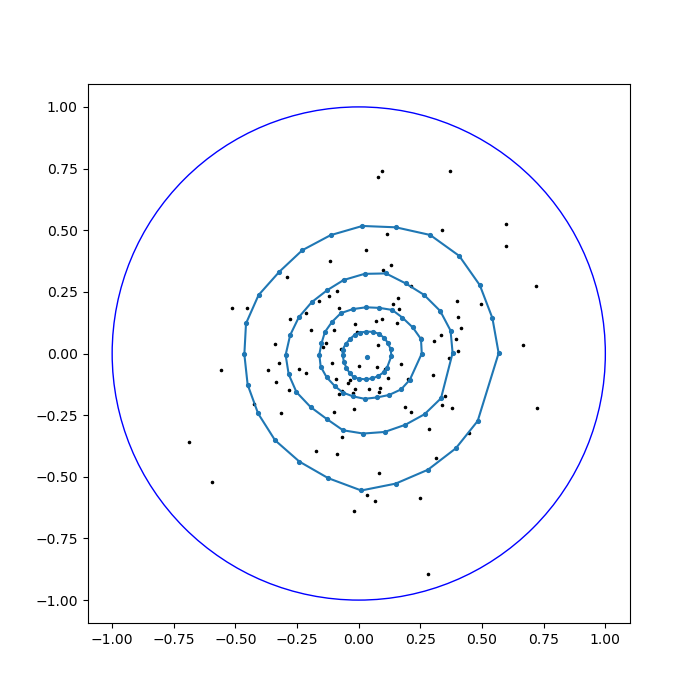
Figure 1: Data points and iso-quantile contours in the synthetic data set.

The results are shown in Figure 1. The black dots are the data points, the blue dots are the sample quantiles, and the blue curves represent iso-quantile contours. The quantiles provide a good idea of the shape of the data cloud. In particular, the gaps between consecutive iso-quantile contours increase significantly with $\beta$, so the distances increase without bound as one approaches the topological boundary of the ball. This is consistent with our expectations for this distribution.

We also tried some of the outlier detection methods in Section 6. Using the same 24 $\xi$ values as above, we first calculated the sample $(\beta,\xi)$-quantiles for $\beta=0.5$, which correspond to quartiles in the univariate case, and drew the iso-quantile contour $Q_{0.5}$. Using this information and the geometric median, we drew the outlier detection fence of (9), and the outlier detection fence $Q_{0.98}$ based on the sample $(\beta,\xi)$-quantiles for $\beta=0.98$ and the same 24 $\xi$ values. These results are shown in Figure 2.

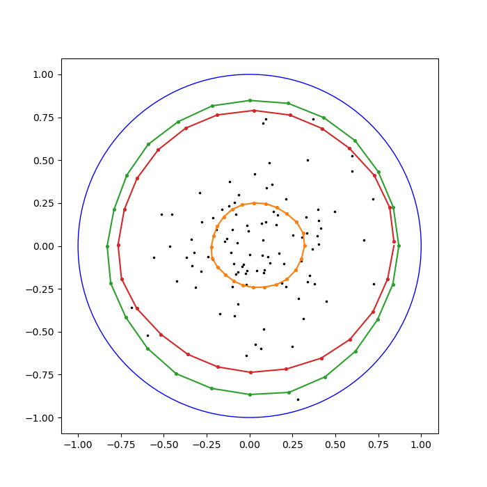
Figure 2: Data points, the iso-quantile contour $Q_{0.5}$ and fences for outlier detection in the synthetic data set.

The orange curve represents the iso-quantile contour $Q_{0.5}$ and gives an idea of what might be called the interquartile range of this data. According to the red curve representing the outlier detection fence in (9), there are four outliers out of 100 points. This number may seem high, but it makes sense when one considers that in the Poincaré ball model, distances increase hyperbolically as one approaches the boundary and that, therefore, those four points are extremely far away from the rest of the data points. According to the green curve representing the alternative outlier detection fence $Q_{0.98}$, there is one outlier. The issues with extreme geometric quantiles and this outlier detection method are less relevant in this case because the data are spherically symmetric.

7.2 Real data experiment

We consider a data set from Olsson et al. (2016) that performed single-cell RNA sequencing (scRNAseq) to analyze ‘discrete genomic states and the transitional intermediates that span myelopoiesis.’ Single-cell RNA sequencing is useful for ‘delineating hierarchical cellular states, including rare intermediates and the networks of regulatory genes that orchestrate cell-type specification,’ a central task in modern developmental biology. These complex hierarchical structures make scRNAseq data ideal for embedding into hyperbolic space. The data have been embedded into the two-dimensional Poincaré disk by Chien et al. (2021) following the procedure in Klimovskaia (2020). The raw data are available at https://github.com/facebookresearch/PoincareMaps/blob/main/datasets/Olsson.csv, and the processed data in the Poincaré disk are available at https://github.com/thupchnsky/PoincareLinearClassification/blob/main/embedding/olsson_poincare_embedding.npz. There, the data are split into train and test sets, and in this analysis, we have combined into a single set of 319 measurements on eight cell types.

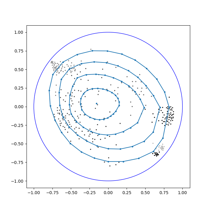
Figure 3: Data points and iso-quantile contours in the real data set.

We used the exact same algorithms as in the simulation experiment. The first results are shown in Figure 3, where the blue curves and the dots on them are iso-quantile contours and quantiles, and the black and gray points are the data. Not that the different shades of black and gray represent different cell types. For smaller values of $\beta$, the quantiles match the shape of the data well. However, looking at the quantiles for $\beta=0.8$, we find a hint of the problem associated with extreme quantiles observed by Girard and Stufler (2017) in Euclidean space and mentioned in Section 6. As $\beta=0.8$ is not too extreme, the problem is not too noticeable in this example. Still, we observe that, roughly along the top-left-to-bottom-right diagonal, many data points fall outside the $\beta=0.8$ contour. In contrast, roughly along the bottom-left-to-top-right diagonal, there are no such points despite the greater variance in the first direction than the second. One might have hoped that the iso-quantile contours would extend further in the first direction and contract in the second. This phenomenon did not appear in the simulation experiment where the distribution is spherically symmetric.

The color scheme of the curves in Figure 4 is analogous to that of Figure 3. The iso-quantile contour $Q_{0.5}$ in orange again gives an idea of an ‘interquartile range’. The outlier detection fence of (9) in red indicates that there are no outliers in the data set, while the alternative outlier detection fence $Q_{0.98}$ designates several points as outliers. However, all the outliers are roughly along the top-left-to-bottom-right diagonal, which hints that there may be a problem with using $Q_{0.98}$. Due to the anisotropic dispersion of the data, the aforementioned problems associated with extreme quantiles are much more pronounced with $Q_{0.98}$ than with $Q_{0.8}$ in Figure 3. Therefore, one must be extra careful when using $Q_{0.98}$ for outlier detection. The red fence appears to have a similar problem, but this may be an optical illusion caused by the extreme distortions near the boundary of the Poincaré ball model. The red curve actually extends considerably further in the rough direction of the top-left-to-bottom-right diagonal than in the direction of the perpendicular diagonal, and unlike the green fence, it does not have a concentration of outliers in specific directions.

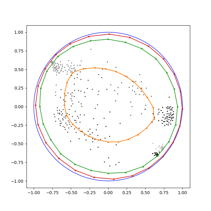
Figure 4: Data points, the iso-quantile contour $Q_{0.5}$ and fences for outlier detection in the real data set.

8 Conclusion

In this paper, we generalize the notion of multivariate geometric quantiles to global non-positive curvature spaces with a bound at infinity. After showing some basic properties, notably scaled isometry equivariance and a necessary condition on Hadamard manifolds for the gradient of the quantile loss function at quantiles, we investigated the large-sample properties of sample quantiles on Hadamard manifolds, specifically a strong law of large numbers and joint asymptotic normality. We also provided an explicit expression for the gradient of the quantile loss function and other details necessary to perform the gradient descent algorithm on hyperbolic spaces.

Considering the plethora of work built upon Chaudhuri (1996) on multivariate geometric quantiles, there are plenty of potential avenues for fruitful research just by generalizing these works to Hadamard space settings. Possible areas of such research include quantile regression, extreme quantiles, geometric expectiles, and, as already mentioned, a procedure for transforming and retransforming data in such a way to produce extreme quantiles that better follow the shape of the distribution, which in turn allows for better detection of outliers using iso-quantiles contours. In addition to these generalizations, it would be beneficial to devise an algorithm to compute quantiles in spaces other than hyperbolic spaces.

Appendix

Appendix A Proofs

A.1 Proof of Proposition 3.3

Proof.

(a) Note that $\gamma$ and $\gamma_{1}$, defined by $\gamma_{1}(t)=\exp_{p}(t\xi_{p})$, are asymptotic. From Section 1.4.1 of Shiga (1984), $d(\gamma(t),\gamma_{1}(t))$ is convex in $t$. Therefore, if it increases at any point, it must be unbounded, which is impossible because the two geodesics are asymptotic, and so, $d(\gamma(t),\gamma_{1}(t))$ is monotonically non-increasing in $t$. Thus, for all $t\geq 0$,

$$t\bigg{\lVert}\frac{\log_{q}(\gamma(t))}{\lVert\log_{p}(\gamma(t))\rVert}-\xi_{p}\bigg{\rVert}=\lVert\log_{p}(\gamma(t))-\log_{p}(\gamma_{1}(t))\rVert\leq d(\gamma(t),\gamma_{1}(t))\leq d(\gamma(0),p),$$

where norms are taken in the tangent space at $p$. The first inequality follows from a condition equivalent to the CAT(0) inequality (see Proposition 1.7(5) in Bridson and Haefliger (1999)). The result follows by dividing by $t$ and sending it to infinity.

(b) Because geodesics corresponding to all $(p,v)\in TM$ can be defined on the entire real line, the geodesic flow on $TM$ (see Definition 2.4 in Ch. 3 of do Carmo (1992)) defined by $\theta(t,p,v)=(\gamma_{p,v}(t),\dot{\gamma}_{p,v}(t))$, where $\gamma_{p,v}(t):=\exp_{p}(tv)$, can be defined on all of $\mathbb{R}\times TM$ and it is smooth on this entire domain by the fundamental theorem on flows (Theorem 9.12 in Lee (2012)). Then, since $\exp(p,v)=\pi(\theta(1,p,v))=\exp_{p}(v)$, where $\pi:TM\rightarrow M$ is the projection map, $\exp$ is also smooth.

Since $\exp_{p}$ is a diffeomorphism between $T_{p}M\cong\mathbb{R}^{n}$ and $M$, the determinant of the differential of the smooth map $(p,v)\mapsto(p,\exp(p,v))$ from $TM$ to $M\times M$ is

$$\det\begin{bmatrix}I&O\\ A&d\exp_{p}\end{bmatrix}=\det(I)\det(d\exp_{p})\neq 0,$$

where $d\exp_{p}$ is identified with its matrix representation in local coordinates and $A$ is some $n\times n$ matrix; thus this map is a local diffeomorphism by the inverse function theorem. Since the inverse of the map exists and is precisely $(p,x)\mapsto(p,\log_{p}(x))$, it is a diffeomorphism. ∎

A.2 Proof of Proposition 3.4

Proof.

(a) The triangle inequality and $\rho(x,p;\beta,\xi)\in[(1-\beta)d(p,x),(1+\beta)d(p,x)]$ imply

$$G^{\beta,\xi}(p) \leq(1+\beta)E[d(p,X)]$$

$$\leq(1+\beta)E[d(p,p^{*})+d(p^{*},X)]$$

$$\leq(1+\beta)\bigg{(}d(p,p^{*})+\frac{1}{1-\beta}E[\rho(X,p^{*};\beta,\xi)]\bigg{)}$$

$$\leq(1+\beta)\bigg{(}d(p,p^{*})+\frac{1}{1-\beta}G^{\beta,\xi}(p^{*})\bigg{)}$$

$$<\infty.$$ (10)

So, both $G^{\beta,\xi}(p)$ and $E[d(p,x)]$ are finite for all $p\in M$.

For any sequence $\{p_{j}\}$ that converges to $p$, there exists some $J<\infty$ such that for all $j_{1},j_{2}\geq J$, $d(p_{j_{1}},p_{j_{2}})<1$. Define a random variable $Y=(1+\beta)(1+\sum_{k=1}^{J}d(p_{k},X))$. Then, $\rho(X,p_{j};\beta,\xi)\leq Y$ for all $j<J$ and

$$\rho(p_{j},X;\beta,\xi) \leq(1+\beta)d(p_{j},X)$$

$$\leq(1+\beta)(d(p_{j},p_{J})+d(p_{J},X))$$

$$<(1+\beta)(1+d(p_{J},X))$$

$$\leq Y$$

for all $j\geq J$. Thus, $\{\rho(X,p_{j};\beta,\xi)\}_{j}$ is dominated by $Y$ and $EY<\infty$ by (A.2). $\rho(x,\cdot;\beta,\xi)$ is also known to be continuous as a function of its second argument (Proposition 3.3(b)). So, $\rho(X,p_{j};\beta,\xi)\rightarrow\rho(X,p;\beta,\xi)$, and $G^{\beta,\xi}(p_{j})\rightarrow G^{\beta,\xi}(p)$ by the dominated convergence theorem; thus, $G^{\beta,\xi}$ is continuous.

(b) Letting $a:=\inf_{p\in M}G^{\beta,\xi}(p)$, there exists by continuity of $G^{\beta,\xi}$ a sequence $\{q_{j}\}$ such that $G^{\beta,\xi}(q_{j})$ goes to $a$. Then, $\{G^{\beta,\xi}(q_{n})\}$ is a bounded sequence. By the triangle inequality, $d(q_{1},q_{j})\leq d(q_{1},X)+d(X,q_{j})\leq(\rho(X,q_{1};\beta,\xi)+\rho(X,q_{j};\beta,\xi))/(1-\beta)$, and taking expected values gives

$$d(q_{1},q_{j})\leq\frac{G^{\beta,\xi}(q_{1})+G^{\beta,\xi}(q_{j})}{1-\beta}.$$ (11)

This and the boundedness of $\{G^{\beta,\xi}(q_{j})\}$ imply that $\{q_{j}\}$ is also bounded. Hadamard spaces are complete, so the bounded sequence $\{p_{j}^{\prime}\}_{j}$ has a subsequence $\{q_{j^{\prime}}\}$ that converges to some $q^{\prime}$. $\{G^{\beta,\xi}(q_{j^{\prime}})\}$ converges to $a$, so by the continuity of $G^{\beta,\xi}$, $G^{\beta,\xi}(q^{\prime})=a$ and the quantile set is nonempty. Since the quantile set is the preimage of the closed set $\{a\}$ under the continuous $G^{\beta,\xi}$, it is also closed. Replacing $q_{1}$ and $q_{j}$ in (11) with $q^{\prime}$ and any minimizer $m\in(G^{\beta,\xi})^{-1}(a)$, $d(q^{\prime},m)\leq 2a/(1-\beta)$, so $(G^{\beta,\xi})^{-1}(\xi)$ is bounded too. Therefore, it is compact as connected Riemannian manifolds are proper. ∎

A.3 Proof of Theorem 3.1

Proof.

Take an $h\in T_{q}M$ such that $\lVert h\rVert=1$ and let $\gamma_{q,h}(t)=\mathrm{exp}_{q}(th)$. We suppress the $q$ and $h$ parameters in the notation for $\gamma_{q,h}$. $\rho$ is differentiable as a function of its second argument on $M\backslash\{x\}$. So, if $x\neq q$,

$$\lim_{t\rightarrow 0+}\frac{\rho(x,\gamma(t);\beta,\xi)-\rho(x,\gamma(0);\beta,\xi)}{t}=d\rho(x,\cdot;\beta,\xi)_{q}(h)=\langle\mathrm{grad}\text{ }\rho(x,q;\beta,\xi),h\rangle.$$ (12)

If $x=q$,

$$\lim_{t\rightarrow 0+}\frac{\rho(x,\gamma(t);\beta,\xi)-\rho(x,\gamma(0);\beta,\xi)}{t} =\lim_{t\rightarrow 0+}\frac{\lVert th\rVert+\langle\beta\xi_{\gamma(t)},\mathrm{log}_{\gamma(t)}(x)\rangle-0}{t}$$

$$=\lim_{t\rightarrow 0+}\frac{t+\langle\beta\xi_{\gamma(t)},-t\gamma^{\prime}(t)\rangle}{t}$$

$$=1-\langle\beta\xi_{q},h\rangle,$$ (13)

where we used continuity in the last equality.

Take any sequence of positive numbers $t_{1},t_{2},\ldots$ that converges to 0. Fixing $j\in\mathbb{Z}_{+}$, if $x=\gamma(t^{\prime})$ for some $t^{\prime}\in(0,t_{j})$,

$$\frac{\lvert\rho(x,\gamma(t_{j});\beta,\xi)-\rho(x,\gamma(0);\beta,\xi)\rvert}{t_{j}}$$

$$\leq~{}\frac{\lvert d(\gamma(t_{j}),\gamma(t^{\prime}))+\langle\log_{\gamma(t_{j})}(\gamma(t^{\prime})),\xi_{\gamma(t_{j})}\rangle\rvert+\lvert d(\gamma(0),\gamma(t^{\prime}))+\langle\log_{\gamma(0)}(\gamma(t^{\prime})),\xi_{\gamma(0)}\rangle\rvert}{t_{j}}$$

$$\leq~{}\frac{|t_{j}-t^{\prime}\rvert\lVert h\rVert+\lvert t_{j}-t^{\prime}\rvert\lVert h\rVert\lVert\xi_{\gamma(t_{j})}\rVert+|t^{\prime}\rvert\lVert h\rVert+\lvert t^{\prime}\rvert\lVert h\rVert\lVert\xi_{\gamma(0)}\rVert}{t_{j}}$$

$$\leq~{}4;$$

otherwise, by the mean value theorem, there exists some $t^{\prime}\in(0,t_{j})$ for which

$$\frac{\lvert\rho(x,\gamma(t_{j});\beta,\xi)-\rho(x,\gamma(0);\beta,\xi)\rvert}{t_{j}} =\lvert\langle\mathrm{grad}\text{ }\rho(x,\gamma(t^{\prime});\beta,\xi),\dot{\gamma}(t^{\prime})\rangle\rvert$$

$$\leq\lVert\mathrm{grad}\text{ }\rho(x,\gamma(t^{\prime});\beta,\xi)\rVert$$

$$\leq\frac{\lVert-\log_{\gamma(t^{\prime})}(x)\rVert}{\lVert\log_{\gamma(t^{\prime})}(x)\rVert}+\lVert R(\gamma(t^{\prime}),x)\rVert$$

$$=1+\lVert R(\gamma(t^{\prime}),x)\rVert,$$

where $R(p,x)$ is the gradient of $\langle\beta\xi_{p},\log_{p}(x)\rangle$ as a function of $p$. Note that $\lVert R(p,x)\rVert$ is continuous as a function of $(p,x)$ by Proposition 3.3(b). Then, $A:=\{(p,x):d(q,p)\leq\sup_{j\in\mathbb{Z}_{+}}t_{j},~{}x\text{ is in the compact support of the distribution of $X$}\}$ is a compact subset of $M\times M$, and so $\sup_{(p,x)\in A}\lVert R(p,x)\rVert<\infty$. Thus, for all $j\in\mathbb{Z}_{+}$.

$$\frac{\lvert\rho(X,\gamma(t_{j});\beta,\xi)-\rho(X,\gamma(0);\beta,\xi)\rvert}{t_{j}}\leq 5+\sup_{(p,x)\in A}\lVert R(p,x)\rVert<\infty$$ (14)

almost surely.

Therefore, we have the following, in which the first equality follows from (14) and the bounded convergence theorem and the second-to-last from (12) and (A.3):

$$\lim_{t\rightarrow 0+}\frac{G^{\beta,\xi}(\gamma(t))-G^{\beta,\xi}(\gamma(0))}{t}$$

$$=E\bigg{[}\lim_{t\rightarrow 0+}\frac{\rho(X,\gamma(t);\beta,\xi)-\rho(X,\gamma(0);\beta,\xi)}{t}\bigg{]}$$

$$=E\bigg{[}\lim_{t\rightarrow 0+}\frac{\rho(X,\gamma(t);\beta,\xi)-\rho(X,\gamma(0);\beta,\xi)}{t};X\neq q\bigg{]}$$

$$\qquad\qquad+E\bigg{[}\lim_{t\rightarrow 0+}\frac{\rho(X,\gamma(t);\beta,\xi)-\rho(X,\gamma(0);\beta,\xi)}{t};X=q\bigg{]}$$

$$=E[\langle\mathrm{grad}\text{ }\rho(X,q;\beta,\xi),h\rangle;X\neq q]+E[1-\langle\beta\xi_{q},h\rangle;X=q]$$

$$=\langle E[\mathrm{grad}\text{ }\rho(X,q;\beta,\xi);X\neq q],h\rangle+P(X=q)(1-\langle\beta\xi_{q},h\rangle),$$

and because $q$ is a minimizer, this quantity must be at least 0 for all $h\in T_{q}M$ such that $\lVert h\rVert=1$; that is, $\langle E[\mathrm{grad}\text{ }\rho(X,q;\beta,\xi);X\neq q]-P(X=q)\beta\xi_{q},-h\rangle\leq P(X=q)$ for all such $h$, which is equivalent to (5). ∎

Proof of Corollary 3.1.

This follows directly from Theorem 3.1 by letting $X$ be the random element that follows the empirical distribution determined by $X_{1},\ldots,X_{N}$ and dividing (5) by $N$. ∎

A.4 Proof of Lemma 4.1

Proof.

$G^{\beta,\xi}$ is finite on all $M$ by Proposition 3.4. Denote by $C(L)$ the vector space of continuous functions on $L$ equipped with the uniform (sup) norm (i.e., for $f\in C(L)$, $\lVert f\rVert:=\sup_{p\in L}\lvert f(p)\rvert$), which is a Banach space; because $L$ is a compact metric space, the Stone-Weierstrass theorem implies that $C(L)$ is separable. Then, the restrictions $\hat{G}^{\beta,\xi}_{N}|_{L}$ and $G^{\beta,\xi}|_{L}$ to $L$ are in $C(L)$ by Proposition 3.4. Note that if $d(x,x^{\prime})<\epsilon/(1+\beta)$, then

$$\lVert\rho(x,\cdot;\beta,\xi)-\rho(x^{\prime},\cdot;\beta,\xi)\rVert \leq\sup_{p\in L}(\lvert d(p,x)-d(p,x^{\prime})\rvert+\lvert\langle\beta\xi_{p},\log_{p}(x)-\log_{q}(x^{\prime})\rangle\rvert)$$

$$\leq\sup_{p\in L}(d(x,x^{\prime})+\lVert\beta\xi_{p}\rVert\lVert\log_{p}(x)-\log_{p}(x^{\prime})\rVert)$$

$$\leq\sup_{p\in L}(d(x,x^{\prime})+\beta d(x,x^{\prime}))$$

$$<\epsilon,$$

where the second inequality follows from the triangle and Cauchy-Schwarz inequalities and the third from a condition equivalent to the CAT(0) inequality (see Proposition 1.7(5) in Bridson and Haefliger (1999)). So, the function from $M\rightarrow C(L)$ defined by $x\rightarrow\rho(x,\cdot;\beta,\xi)$ is continuous, and hence, measurable, as a function of its first argument into $C(L)$ equipped with its induced Borel $\sigma$-algebra. Therefore, $\rho(X,\cdot;\beta,\xi)$, and hence, each $\hat{G}^{\beta,\xi}_{N}|_{L}$, is a $C(L)$-valued random element. For any fixed $p^{\prime}\in L$ and noting $\mathrm{diam}(L):=\sup_{p,p_{0}\in L}d(p,p_{0})<\infty$ by the compactness, and hence, the boundedness, of $L\subset M$,

$$E[\lVert\rho(X,\cdot;\beta,\xi)\rVert] =E\bigg{[}\sup_{p\in L}\rho(p,X;\beta,\xi)\bigg{]}$$

$$\leq E\bigg{[}\sup_{p\in L}(1+\beta)d(p,X)\bigg{]}$$

$$\leq E\bigg{[}\sup_{p\in L}(1+\beta)(d(p,p^{\prime})+d(p^{\prime},X))\bigg{]}$$

$$\leq E\bigg{[}(1+\beta)(\mathrm{diam}(L)+d(p^{\prime},X))\bigg{]}$$

$$\leq(1+\beta)\mathrm{diam}(L)+(1+\beta)E\bigg{[}\frac{\rho(X,p^{\prime};\beta,\xi)}{1-\beta}\bigg{]}$$

$$=(1+\beta)\mathrm{diam}(L)+\frac{1+\beta}{1-\beta}G^{\beta,\xi}(p^{\prime})|_{L}$$

$$<\infty$$

by Proposition 3.4. Then, by the strong law of large numbers on separable Banach spaces (see Mourier (1953) or Theorem 4.1.1 in Padgett and Taylor (1973)), $\lVert\hat{G}^{\beta,\xi}_{N}|_{L}-G^{\beta,\xi}|_{L}\rVert\rightarrow 0$ almost surely, from which the desired result follows. ∎

A.5 Proof of Theorem 4.1

Proof.

$G^{\beta,\xi}$ is finite on all $M$ by Proposition 3.4. Recalling that $q(\beta,\xi)$ is nonempty by Proposition 3.4, define $l$ to be $G^{\beta,\xi}(q)$ for any $q\in q(\beta,\xi)$, that is, $l=\min\{G^{\beta,\xi}(p):p\in M\}$. We first show that there exist some compact $D\subset M$, $\Omega_{2}\in\mathcal{F}$ of $P$-measure 1 and an $N_{2}(\omega)<\infty$ for each $\omega\in\Omega_{2}$ for which $N\geq N_{2}(\omega)$ implies that

$$\hat{G}^{\beta,\xi}_{N}(p)>l+1$$ (15)

for all $p\in M\backslash D$.

For a fixed $q\in q(\beta,\xi)$,

$$\hat{G}^{\beta,\xi}_{N}(p) \geq(1-\beta)\frac{1}{N}\sum_{i=1}^{N}d(p,X_{i})$$

$$\geq(1-\beta)\frac{1}{N}\sum_{i=1}^{N}\lvert d(p,q)-d(q,X_{i})\rvert$$

$$\geq(1-\beta)\frac{1}{N}\sum_{i=1}^{N}(d(p,q)-d(q_{0},X_{i}))$$

$$\geq(1-\beta)\bigg{(}d(p,q)-(1+\beta)\frac{1}{N}\sum_{i=1}^{N}\rho(X_{i},q;\beta,\xi)\bigg{)}$$

$$=(1-\beta)(d(p,q)-(1+\beta)\hat{G}^{\beta,\xi}_{N}(q)).$$ (16)

By $G^{\beta,\xi}(q)=l<\infty$ and the almost sure convergence of $\hat{G}^{\beta,\xi}_{N}(q)$ to $G^{\beta,\xi}(q)$, there exist some $\Omega_{2}\in\mathcal{F}$ of $P$-measure 1 and an $N_{2}(\omega)<\infty$ for all $\omega\in\Omega_{2}$ for which $N\geq N_{2}(\omega)$ implies that $\hat{G}^{\beta,\xi}_{N}(q)<l+1$. Then, by (A.5), for $\Delta:=(l+1)(1/(1-\beta)+1+\beta)$, $d(q,q_{0})>\Delta$, $\omega\in\Omega_{2}$ and $N\geq N_{2}(\omega)$ imply $\hat{G}^{\beta,\xi}_{N}(q)>l+1$. Then, defining $D:=\{p:d(p,q(\beta,\xi))\leq\Delta\}\supset{\{p:d(p,q)\leq\Delta\}}$, which is closed and bounded and hence compact by the properness of $M$, $N\geq N_{2}(\omega)$ implies that $\hat{G}^{\beta,\xi}_{N}(p)>l+1$ for all $p\in M\backslash D$, so we have found the desired compact $D$.

If there exist some $\theta(\epsilon)>0$, $\Omega_{1}\in\mathcal{F}$ of $P$-measure 1 and $N_{1}(\omega)<\infty$ for all $\omega\in\Omega_{1}$ such that $N\geq N_{1}(\omega),\omega\in\Omega_{1}$, implies

$$\hat{G}^{\beta,\xi}_{N}(p)\leq l+\frac{\theta(\epsilon)}{2}\qquad\text{ for all $p\in q(\beta,\xi)$, and}$$

$$\hat{G}^{\beta,\xi}_{N}(p)\geq l+\theta(\epsilon)\qquad\text{ for all $p\in M\backslash C^{\epsilon}$},$$ (17)

then no minimizer of $\hat{G}^{\beta,\xi}_{N}$, that is, no element of the sample $(\beta,\xi)$-quantile set defined in the statement of the theorem, is in $M\backslash C^{\epsilon}$ if $\omega\in\Omega_{1}$ and $N\geq N_{1}(\omega)$, proving part (a) of the theorem.

$D_{\epsilon}:=D\cap(M\backslash C^{\epsilon})$, being the intersection of a closed and bounded set and a closed one, is itself closed and bounded and hence compact because $M$ is a proper metric space. By continuity, $G^{\beta,\xi}$ attains its minimum $l_{\epsilon}:=\min\{G^{\beta,\xi}(p):p\in D_{\epsilon}\}$ on the compact $D_{\epsilon}$, and since $D_{\epsilon}\cap q(\beta,\xi)$ is empty, $l_{\epsilon}>l$, so there is some $\theta(\epsilon)\in(0,1)$ such that $l_{\epsilon}>l+2\theta(\epsilon)$. We now use Lemma 4.1 for $K=D$, allowing us to find a set $\Omega_{3}\in\mathcal{F}$ and $N_{3}(\omega)<\infty$ for each $\omega\in\Omega_{3}$ such that $N\geq N_{3}(\omega)$ implies that $\sup_{p\in D}\lvert\hat{G}^{\beta,\xi}_{N}(p)-G^{\beta,\xi}(p)\rvert<\theta(\epsilon)/2$, and thus $\hat{G}^{\beta,\xi}_{N}(p)\leq G^{\beta,\xi}(p)+\theta(\epsilon)/2=l+\theta(\epsilon)/2$ for all $p\in q(\beta,\xi)\subset D$, satisfying the first part of (A.5), and $\hat{G}^{\beta,\xi}_{N}(p)>G^{\beta,\xi}(p)-\theta(\epsilon)/2>l_{\epsilon}-2\theta(\epsilon)/2>l+\theta(\epsilon)$ for all $p\in D_{\epsilon}\subset D$. This and (15) imply that $\hat{G}^{\beta,\xi}_{N}(p)>l+\theta(\epsilon)$ for all $p\in D_{\epsilon}\cup(M\backslash D)\supset M\backslash C^{\epsilon}$ if $N\geq N_{1}(\omega)$ and $\omega\in\Omega_{1}$, where $\Omega_{1}=\Omega_{2}\cap\Omega_{3}$ and $N_{1}(\omega)=\max\{N_{2}(\omega),N_{3}(\omega)\}$, satisfying the second part of (A.5) and completing the proof of part (a). The proposed convergences in part (b) hold for all $\omega\in\Omega_{1}$, and $P(\Omega_{1})=1$, proving part (b). ∎

A.6 Proofs of Theorem 4.2 and its corollaries

The proof will require the following two lemmas.

Lemma A.1.

Let $M$ be an $n$-dimensional $(n\geq 2)$ Hadamard manifold.

• There exists a positive upper semi-continuous function $L:M\times M\rightarrow\mathbb{R}$ that satisfies

  $$\lVert x-p\rVert_{2}=L(x,p)\lVert\log_{p}(x)\rVert_{g}.$$

• There exists a positive upper semi-continuous function $S:M\times M\rightarrow\mathbb{R}$ that satisfies

  $$\lvert D_{r^{\prime}}\Psi^{r}(x,p;0,\xi)\rvert \leq\frac{S(x,p)}{\lVert x-p\rVert_{2}},$$

  for all $r,r^{\prime}=1,\ldots,n$ whenever $x\neq p$.

Proof.

(a) Consider the geodesic (according to the metric $g$) $\gamma_{p,x}:[0,1]\rightarrow M$ satisfying $\gamma_{p,x}(0)=p$, $\gamma_{p,x}(1)=x$. Denoting by $\zeta_{\min}(p)$ the smallest eigenvalue of $g_{p}$, $\zeta_{\min}$ is continuous as a function of $p$ because eigenvalues are the roots of polynomials whose coefficients are continuous functions of the entries of a matrix. Then define $\zeta_{\inf}(x,p):=\inf_{t\in[0,1]}\zeta_{\min}(\gamma_{p,x}(t))$. The length of the curve $\gamma_{p,x}$ measured in the Euclidean metric must be at least as large as the length of the straight line from $p$ to $x$, so

$$\sqrt{\zeta_{\inf}(x,p)}\lVert x-p\rVert_{2} \leq\sqrt{\zeta_{\inf}(x,p)}\int_{0}^{1}\lVert\dot{\gamma}_{p,x}(t)\rVert_{2}dt$$

$$\leq\int_{0}^{1}\sqrt{\dot{\gamma}_{p,x}^{T}g_{\gamma_{p,x}(t)}\dot{\gamma}_{p,x}}dt$$

$$=\int_{0}^{1}\lVert\dot{\gamma}_{p,x}(t)\rVert_{g}dt$$

$$=d(p,x)$$

$$=\lVert\log_{p}(x)\rVert_{g},$$

or

$$\frac{\lVert x-p\rVert_{2}}{\lVert\log_{p}(x)\rVert_{g}}\leq\frac{1}{\sqrt{\zeta_{\inf}(x,p)}}$$

if $x\neq p$. Fix some $p^{\prime}\in M$. By the continuity of $\zeta_{\min}$, there exists for any for any $\epsilon>0$ some $\delta>0$ for which $d(p,p^{\prime})<\delta$ implies $\lvert 1/\sqrt{\zeta_{\min}(p)}-1/\sqrt{\zeta_{\min}(p^{\prime})}\rvert<\epsilon$. All geodesic balls are convex on Hadamard manifolds, and because the image of $\gamma_{p,x}$ is compact, $\zeta_{\inf}(p,x)=\zeta_{\min}(\gamma_{p,x}(t))>0$ for some $t\in[0,1]$. Therefore, if $d(p,p^{\prime})<\delta$ and $d(x,p^{\prime})<\delta$, $d(p^{\prime},\gamma_{p,x}(t))<\delta$ and $\lvert 1/\sqrt{\zeta_{\inf}(p,x)}-1/\sqrt{\zeta_{\min}(p^{\prime})}\rvert<\epsilon$. This means that

$$\lim\sup_{(x,p)\rightarrow(p^{\prime},p^{\prime})}\frac{\lVert x-p\rVert_{2}}{\lVert\log_{p}(x)\rVert_{g}}\leq\lim_{(x,p)\rightarrow(p^{\prime},p^{\prime})}\frac{1}{\sqrt{\zeta_{\inf}(x,p)}}=\frac{1}{\sqrt{\zeta_{\min}(p^{\prime})}}.$$ (18)

Then, $L(x,p)$ defined by

$$L(x,p)=\begin{cases}\frac{\lVert x-p\rVert_{2}}{\lVert\log_{p}(x)\rVert_{g}}&~{}~{}\mbox{if $x\neq p$}\\ \frac{1}{\sqrt{\zeta_{\min}(p)}}&~{}~{}\mbox{if $x=p$}\end{cases}$$

is continuous if $x\neq p$, while the upper semi-continuity at $(p,p)\in M\times M$ follows from (18) and the continuity of $1/\sqrt{\zeta_{\min}(p)}$ on $M$.

(b) The Euclidean gradient of $\lVert\log_{p}(x)\rVert_{g}$ as a function of $p$ is $\Psi(x,p;0,\xi)=-g_{p}\log_{p}(x)/\lVert\log_{p}(x)\rVert_{g}$ when $x\neq p$. Thus, the Euclidean Hessian matrix of the same function at $x\neq p$ is

$$[D_{r}^{\prime}\Psi^{r}(x,p;0,\xi)]_{r,r^{\prime}=1,\ldots,n} =\frac{S^{*}(x,p)\lVert\log_{p}(x)\rVert_{g}-(g_{p}\log_{p}(x))(g_{p}\log_{p}(x))^{T}/\lVert\log_{p}(x)\rVert_{g}}{\lVert\log_{p}(x)\rVert_{g}^{2}}$$

$$=\frac{S^{*}(x,p)-(g_{p}\log_{p}(x))(g_{p}\log_{p}(x))^{T}/\lVert\log_{p}(x)\rVert_{g}^{2}}{\lVert\log_{p}(x)\rVert_{g}}$$

for some $n\times n$ matrix function $S^{*}(x,p)$ that is smooth on all of $M\times M$ (by the smoothness of $g_{p}\log_{p}(x)$). Denoting the smallest and largest eigenvalues of $g_{p}$ by $\zeta_{\min}(p)$ and $\zeta_{\max}(p)$, respectively, these are continuous on all of $M$ as functions of $p$, $\zeta_{\max}(p)\geq\zeta_{\min}(p)>0$ by positive definiteness,

$$\lVert\log_{p}(x)\rVert_{g}^{2}=\log_{p}(x)^{T}g_{p}\log_{p}(x)\in\big{[}\zeta_{\min}(p)\lVert\log_{p}(x)\rVert_{2}^{2},~{}\zeta_{\max}(p)\lVert\log_{p}(x)\rVert_{2}^{2}\big{]},$$ (19)

and

$$(g_{p}\log_{p}(x))^{T}(g_{p}\log_{p}(x))=\log_{p}(x)^{T}g_{p}^{2}\log_{p}(x)\in\big{[}\zeta_{\min}(p)^{2}\lVert\log_{p}(x)\rVert_{2}^{2},~{}\zeta_{\max}(p)^{2}\lVert\log_{p}(x)\rVert_{2}^{2}\big{]}.$$ (20)

Because of this, and because the absolute value of any entry of $S^{*}(x,p)$ is less than or equal to the Frobenius norm of $S^{*}(x,p)$ $\lVert S^{*}(x,p)\rVert_{F}$, and the absolute value of any entry of $(g_{p}\log_{p}(x))(g_{p}\log_{p}(x))^{T}$ is less than or equal to $(g_{p}\log_{p}(x))^{T}(g_{p}\log_{q}(x))$,

$$\lvert D_{r}^{\prime}\Psi^{r}(x,p;0,\xi)\rvert \leq\frac{\lVert S^{*}(x,p)\rVert_{F}+\zeta_{\max}(p)^{2}\lVert\log_{p}(x)\rVert_{2}^{2}/\zeta_{\min}(p)\lVert\log_{p}(x)\rVert_{2}^{2}}{\lVert x-p\rVert_{2}}\frac{\lVert x-p\rVert_{2}}{\lVert\log_{q}(x)\rVert_{g}}$$

$$=\frac{(\lVert S^{*}(x,p)\rVert_{F}+\zeta_{\max}(p)^{2}/\zeta_{\min}(p))L(x,p)}{\lVert x-p\rVert_{2}}$$

$$=\frac{S(x,p)}{\lVert x-p\rVert_{2}},$$

when $x\neq p$, where $R(x,p)$ is taken from (a) and $S(x,p)$ is a positive real function that is upper semi-continuous on all of $M\times M$. ∎

For $j\in\{2,\infty\}$, we use $u_{k,j}$ defined as

$$u_{k,j}(x,q,d)=\sup_{\tau:\lVert\tau-q\rVert_{2}\leq d}\lVert\Psi_{k}(x,\tau)-\Psi_{k}(x,q)\rVert_{j},$$

and

$$Z_{k,j}(x_{1},\ldots,x_{N},\tau,q)=\frac{\lVert\sum_{i=1}^{N}(\Psi_{k}(x_{i},\tau)-\Psi_{k}(x_{i},q)-\lambda_{k}(\tau)+\lambda_{k}(q))\rVert_{j}}{\sqrt{N}+N\lVert\lambda_{k}(\tau)\rVert_{j}}$$

as in Huber (1967).

Lemma A.2.

Let $M$ be an $n$-dimensional $(n\geq 2)$ Hadamard manifold and fix $q\in M$, $k\in\{1,\ldots,K\}$ and $j\in\{2,\infty\}$. Assume that $A_{j}:=\{\tau:\lVert\tau-q\rVert_{j}\leq d\}\subset M$.

• $u_{k,j}(x,q,d)$ is measurable as a function of $x$.

• Assuming $\lambda_{k}$ is continuous on $A_{j}$, $\sup_{\tau\in A_{j}}Z_{k,j}(x_{1},\ldots,x_{N},\tau,q)$ is measurable as a function of $x_{1}$,…,$x_{N}$.

Proof.

(a) Defining $R(x,p)$ to be the Riemannian gradient of $\langle\beta\xi_{p},\log_{p}(x)\rangle_{g}$ as a function of $p$, $R$ is continuous on $M\times M$. Then, $\Psi_{k}(x,\tau)=-g_{\tau}\log_{\tau}(x)/\lVert\log_{\tau}(x)\rVert_{g}+g_{\tau}R(x,\tau)$ when $x\neq\tau$, and noting that (A.3) contains a proof that $R(x,p)=-\beta\xi_{p}$, $\Psi_{k}(x,\tau)=g_{\tau}R(x,\tau)$ when $x=\tau$.

The map defined by $(p,v)\mapsto(p,\exp_{p}(v))$ for $(p,v)\in TM$ has differential

$$\begin{bmatrix}I&O\\ I&I\end{bmatrix}$$

at $(x,0)\in TM$ since $d(\exp_{x})_{0}=I$. Then its inverse $(p,b)\mapsto(p,\log_{p}(b))$ is smooth by Lemma 3.3(a) and has differential

$$\begin{bmatrix}I&O\\ -I&I\end{bmatrix}$$

at $(x,x)$, so $d(\log_{\cdot}(x))_{x}=-I$.

Then, by Taylor’s theorem for multivariate functions,

$$\log_{\tau}(x) =\log_{x}(x)+d(\log_{\cdot}(x))_{x}(\tau-x)+F(\tau)(\tau-x)$$

$$=(I-F(\tau))(x-\tau),$$

where $F:M\rightarrow\mathbb{R}^{n\times n}$ satisfies $\lim_{\tau\rightarrow x}F(\tau)=0$. Therefore, for any smooth path $c:[0,1]\rightarrow M$ satisfying $c(0)=x$,

$$\frac{\log_{c(t)}(x)}{\lVert\log_{c(t)}(x)\rVert_{2}} =\frac{(I-F(c(t))\frac{(c(0)-c(t))/t}{\lVert(c(0)-c(t))/t\rVert_{2}}}{\Big{\lVert}(I-F(c(t))\frac{(c(0)-c(t))/t}{\lVert(c(0)-c(t))/t\rVert_{2}}\Big{\rVert}_{2}}$$

$$\rightarrow\frac{(I-0)\frac{-\dot{c}(0)}{\lVert-\dot{c}(0)\rVert_{2}}}{\Big{\lVert}(I-0)\frac{-\dot{c}(0)}{\lVert-\dot{c}(0)\rVert_{2}}\Big{\rVert}_{2}}$$

$$=-\frac{\dot{c}(0)}{\lVert\dot{c}(0)\rVert_{2}}$$ (21)

as $t\rightarrow 0$.

Suppose $j=2$. For any $p\in A_{2}$ and vector $v\in\mathbb{R}^{n}$, one can construct a smooth path $c_{2}:[0,1]\rightarrow M$ satisfying $c_{2}(t)=p$ if and only if $t=0$, $c_{2}([0,1])\subset A_{2}$ and $\langle g_{p}\dot{c}_{2}(0),v\rangle_{2}=0$ in the following manner. Take any $w$ that is orthogonal (in the Euclidean inner product) to $v$. If $p$ is in the interior of $A_{2}$, or it is on the boundary $\partial A_{2}$ of $A_{2}$ and $g_{p}^{-1}w$ is not tangent to $\partial A_{2}$, which is diffeomorphic to $S^{n-1}$, at $p$, there exists a possibly negative $a$ that is sufficiently small in absolute value such that $p+ag_{p}^{-1}w\in A_{2}$; this is because if the Euclidean ray from $p$ in the direction of $g_{p}^{-1}w$ is not initially in $A_{2}$, then the Euclidean ray in the direction of $-g_{p}^{-1}w$ is. Then, $c_{2}(t)=p+tag_{p}^{-1}w$ satisfies the desiderata. On the other hand, if $p$ is on $\partial A_{2}$ and $g_{p}^{-1}w$ is tangent to $\partial A_{2}$ at $p$, $c_{2}(t)=\exp_{p}^{\partial A_{2}}(tg_{p}^{-1}w)$, where $\exp_{p}^{\partial A_{2}}$ is the exponential map at $p$ on $\partial A_{2}\cong S^{n-1}$. This $c_{2}$ also satisfies the desiderata.

Suppose that $x\in A_{2}$ and let $p=x$ and $v=\Psi_{k}(x,x)-\Psi_{k}(x,q)$. Then, given (A.6), Lemma A.1(a), the first paragraph of this proof, and the properties of $c_{2}$,

$$\lim\inf_{t\rightarrow 0}\lVert\Psi_{k}(x,c_{2}(t))-\Psi_{k}(x,q)\rVert_{2}^{2}$$

$$=\lim\inf_{t\rightarrow 0}\bigg{\lVert}-g_{c_{2}(t)}\frac{\log_{c_{2}(t)}(x)}{\lVert\log_{c_{2}(t)}(x)\rVert_{g}}+g_{c_{2}(t)}R(x,c_{2}(t))-\Psi_{k}(x,q)\bigg{\rVert}_{2}^{2}$$

$$\geq\lim\inf_{t\rightarrow 0}\bigg{\lVert}-g_{c_{2}(t)}\frac{\log_{c_{2}(t)}(x)}{\lVert\log_{c_{2}(t)}(x)\rVert_{g}}\bigg{\rVert}_{2}^{2}+\lim_{t\rightarrow 0}\lVert g_{c_{2}(t)}R(x,c_{2}(t))-\Psi_{k}(x,q)\rVert_{2}^{2}$$

$$\qquad-2\lim\sup_{t\rightarrow 0}\bigg{\lvert}\bigg{\langle}-g_{c_{2}(t)}\frac{\log_{c_{2}(t)}(x)}{\lVert\log_{c_{2}(t)}(x)\rVert_{g}},g_{c_{2}(t)}R(x,c_{2}(t))-\Psi_{k}(x,q)\bigg{\rangle}_{2}\bigg{\rvert}$$

$$\geq 0+\lVert g_{x}R(x,x)-\Psi_{k}(x,q)\rVert_{2}^{2}$$

$$\qquad-2\lim\sup_{t\rightarrow 0}L(x,c_{2}(t))\bigg{\lvert}\bigg{\langle}-g_{c_{2}(t)}\frac{\log_{c_{2}(t)}(x)}{\lVert\log_{c_{2}(t)}(x)\rVert_{2}},g_{c_{2}(t)}R(x,c_{2}(t))-\Psi_{k}(x,q)\bigg{\rangle}_{2}\bigg{\rvert}$$

$$=\lVert\Psi_{k}(x,x)-\Psi_{k}(x,q)\rVert_{2}^{2}$$

$$\qquad-2\lim\sup_{t\rightarrow 0}L(x,c_{2}(t))\lim_{t\rightarrow 0}\bigg{\lvert}\bigg{\langle}-g_{c_{2}(t)}\frac{\log_{c_{2}(t)}(x)}{\lVert\log_{c_{2}(t)}(x)\rVert_{2}},g_{c_{2}(t)}R(x,c_{2}(t))-\Psi_{k}(x,q)\bigg{\rangle}_{2}\bigg{\rvert}$$

$$\geq\lVert\Psi_{k}(x,x)-\Psi_{k}(x,q)\rVert_{2}^{2}$$

$$\qquad-2L(x,x)\bigg{\lvert}\bigg{\langle}g_{x}\frac{\dot{c}_{2}(0)}{\lVert\dot{c}_{2}(0)\rVert_{2}},g_{x}R(x,x)-\Psi_{k}(x,q)\bigg{\rangle}_{2}\bigg{\rvert}$$

$$=\lVert\Psi_{k}(x,x)-\Psi_{k}(x,q)\rVert_{2}^{2}.$$ (22)

Since $c_{2}(t)=x$ if and only if $t=0$, this proves that $\sup_{\tau\in A_{2}\backslash\{x\}}\lVert\Psi_{k}(x,\tau)-\Psi_{k}(x,q)\rVert_{2}\geq\lVert\Psi_{k}(x,x)-\Psi_{k}(x,q)\rVert_{2}$ if $x\in A_{2}$, and therefore that

$$u_{k,2}(x,q,d)=\sup_{\tau\in A_{2}\backslash\{x\}}\lVert\Psi_{k}(x,\tau)-\Psi_{k}(x,q)\rVert_{2}$$ (23)

for all $x\in M$. There exists a countable set $B:=\{b_{1},b_{2},\ldots\}\subset A_{2}\backslash\{x\}$ for which

$$\sup_{\tau\in B}\lVert\Psi_{k}(x,\tau)-\Psi_{k}(x,q)\rVert_{2}=\sup_{\tau\in A_{2}\backslash\{x\}}\lVert\Psi_{k}(x,\tau)-\Psi_{k}(x,q)\rVert_{2},$$ (24)

and for each $l\in\mathbb{Z}_{+}$ a sequence of points in $A_{2}\backslash\{x\}$ with rational coordinates that converges to $b_{l}$; call the set of points in this sequence $B_{l}$. For all $x\in M$, $\lVert\Psi_{k}(x,\tau)-\Psi_{k}(x,q)\rVert_{2}$ is continuous as a function of $\tau$ on $A_{2}\backslash\{x\}$, so $\lVert\Psi_{k}(x,b_{l})-\Psi_{k}(x,q)\rVert_{2}\leq\sup_{\tau\in B_{l}}\lVert\Psi_{k}(x,\tau)-\Psi_{k}(x,q)\rVert_{2}$, and therefore by (23) and (24), $u_{k,2}(x,q,d)=\sup_{\tau\in B}\lVert\Psi_{k}(x,\tau)-\Psi_{k}(x,q)\rVert_{2}\leq\sup_{\tau\in\cup_{l=1}^{\infty}B_{l}}\lVert\Psi_{k}(x,\tau)-\Psi_{k}(x,q)\rVert_{2}\leq\sup_{\tau\in\mathbb{Q}^{n}\cap A_{2}}\lVert\Psi_{k}(x,\tau)-\Psi_{k}(x,q)\rVert_{2}$, since each $B_{l}$ is a subset of $\mathbb{Q}^{n}\cap A_{2}$. Clearly $u_{k,2}(x,q,d)\geq\sup_{\tau\in\mathbb{Q}^{n}\cap A_{2}}\lVert\Psi_{k}(x,\tau)-\Psi_{k}(x,q)\rVert_{2}$ also holds, so $u_{k,2}(x,q,d)=\sup_{\tau\in\mathbb{Q}^{n}\cap A_{2}}\lVert\Psi_{k}(x,\tau)-\Psi_{k}(x,q)\rVert_{2}$ for all $x\in M$. The desired conclusion follows for $j=2$ since the $\sup$ of countably many measurable functions is measurable.

Now suppose $j=\infty$. Denote by $V$ the set of corners of the hypercube $A_{\infty}$ and by $\pi^{1},\ldots,\pi^{n}:\mathbb{R}^{n}\rightarrow\mathbb{R}$ the projection functions defined by $\pi^{r^{\prime}}(p^{1},\ldots,p^{n})=p^{r^{\prime}}$ for $r^{\prime}=1,\ldots,n$, which are continuous. Choose any $p\in A_{\infty}\backslash\{V\}$ and vector $v\in\mathbb{R}^{n}$. Let $r$ be any index for which $\lvert\pi^{r}(v)\rvert=\lVert v\rVert_{\infty}$ (that is, $r\in\arg\max_{r^{\prime}\in\{1,\ldots,n\}}\lvert\pi^{r^{\prime}}(v)\rvert$). The $(n-1)$-dimensional hyperplane $\{p+g_{p}^{-1}w:\langle w,e^{r}\rangle_{2}=0\}$, where $e^{r}$ is the $r$th standard unit vector, passes through $p\not\in V$ and hence, intersects the hypercube $A_{\infty}$ at some point $y\neq p$ (note that this might not be guaranteed if $p\in V$). Defining $c_{\infty}:[0,1]\rightarrow M$ by $c_{\infty}(t)=p+t(y-p)$, we have that $c_{\infty}(t)=p$ if and only if $t=0$, $c_{\infty}([0,1])\subset A_{\infty}$ and $\langle g_{p}\dot{c}_{\infty}(0),e^{r}\rangle_{2}=0$. Supposing $x\in A_{\infty}\backslash V$ and letting $p=x$ and $v=\Psi_{k}(x,x)-\Psi_{k}(x,q)$, by these properties of $c_{\infty}$, and again by (A.6), Lemma A.1(a) and the first paragraph of this proof,

$$\lim\inf_{t\rightarrow 0}\lVert\Psi_{k}(x,c_{\infty}(t))-\Psi_{k}(x,q)\rVert_{\infty}$$

$$=\lim\inf_{t\rightarrow 0}\bigg{\lVert}-g_{c_{\infty}(t)}\frac{\log_{c_{\infty}(t)}(x)}{\lVert\log_{c_{\infty}(t)}(x)\rVert_{g}}+g_{c_{\infty}(t)}R(x,c_{\infty}(t))-\Psi_{k}(x,q)\bigg{\rVert}_{\infty}$$

$$\geq\lim\inf_{t\rightarrow 0}\bigg{\lvert}\pi^{r}(g_{c_{\infty}(t)}R(x,c_{\infty}(t))-\Psi_{k}(x,q))+\pi^{r}\bigg{(}-g_{c_{\infty}(t)}\frac{\log_{c_{\infty}(t)}(x)}{\lVert\log_{c_{\infty}(t)}(x)\rVert_{g}}\bigg{)}\bigg{\rvert}$$

$$\geq\lim\inf_{t\rightarrow 0}\Bigg{(}\lvert\pi^{r}(g_{c_{\infty}(t)}R(x,c_{\infty}(t))-\Psi_{k}(x,q))\rvert-\bigg{\lvert}\pi^{r}\bigg{(}-g_{c_{\infty}(t)}\frac{\log_{c_{\infty}(t)}(x)}{\lVert\log_{c_{\infty}(t)}(x)\rVert_{g}}\bigg{)}\bigg{\rvert}\Bigg{)}$$

$$\geq\lim_{t\rightarrow 0}\lvert\pi^{r}(g_{c_{\infty}(t)}R(x,c_{\infty}(t))-\Psi_{k}(x,q))\rvert-\lim\sup_{t\rightarrow 0}L(x,c_{\infty}(t))\bigg{\lvert}\pi^{r}\bigg{(}-g_{c_{\infty}(t)}\frac{\log_{c_{\infty}(t)}(x)}{\lVert\log_{c_{\infty}(t)}(x)\rVert_{2}}\bigg{)}\bigg{\rvert}$$

$$=\lvert\pi^{r}(g_{x}R(x,x)-\Psi_{k}(x,q))\rvert-\lim\sup_{t\rightarrow 0}L(x,c_{\infty}(t))\lim_{t\rightarrow 0}\bigg{\lvert}\pi^{r}\bigg{(}-g_{c_{\infty}(t)}\frac{\log_{c_{\infty}(t)}(x)}{\lVert\log_{c_{\infty}(t)}(x)\rVert_{2}}\bigg{)}\bigg{\rvert}$$

$$\geq\lvert\pi^{r}(\Psi_{k}(x,x)-\Psi_{k}(x,q))\rvert-L(x,x)\bigg{\lvert}\pi^{r}\bigg{(}g_{x}\frac{\dot{c}_{\infty}(0)}{\lVert\dot{c}_{\infty}(0)\rVert_{2}}\bigg{)}\bigg{\rvert}$$

$$=\lVert\Psi_{k}(x,x)-\Psi_{k}(x,q)\rVert_{\infty}.$$

Since $c_{\infty}(t)=x$ if and only if $t=0$, this proves that $\sup_{\tau\in A_{\infty}\backslash\{x\}}\lVert\Psi_{k}(x,\tau)-\Psi_{k}(x,q)\rVert_{\infty}\geq\lVert\Psi_{k}(x,x)-\Psi_{k}(x,q)\rVert_{\infty}$ if $x\in A_{\infty}\backslash V$.Now an analogous argument to that of the $j=2$ case shows that for all $x\in M\backslash V$, $u_{k,\infty}(x,q,d)=\sup_{\tau\in\mathbb{Q}^{n}\cap A_{\infty}}\lVert\Psi_{k}(x,\tau)-\Psi_{k}(x,q)\rVert_{\infty}$. Then, noting that $V=\{p_{1},\ldots,p_{2^{n}}\}$ consists of finitely many elements gives

$$u_{k,\infty}(x,q,d) =\bigg{(}\sup_{\tau\in\mathbb{Q}^{n}\cap A_{\infty}}\lVert\Psi_{k}(x,\tau)-\Psi_{k}(x,q)\rVert_{\infty}\bigg{)}I(x\not\in V)+\sum_{l=1}^{2^{n}}u_{k,\infty}(p_{l},q,d)I(x=p_{l}),$$

which is measurable since the $\sup$ of countably many measurable functions is measurable.

(b) This proof is very similar to that of (a), with slight modifications. Fix $i^{\prime}\in\{1,\ldots,N\}$.

Dealing first with the $j=2$ case, suppose $x_{i^{\prime}}\in A_{2}$ and define $c_{2}$ as described in the proof of (a) for $p=x_{i^{\prime}}$ and $v=\sum_{i=1}^{N}(\Psi_{k}(x_{i},x_{i^{\prime}})-\Psi_{k}(x_{i},q)-\lambda_{k}(x_{i^{\prime}})+\lambda_{k}(q))$. Let $N^{\prime}:=\lvert\{i:x_{i}=x_{i^{\prime}},1\leq i\leq N\}\rvert$ be the number of $x_{i}$ which equal $x_{i^{\prime}}$. Recalling the continuity of $\lambda_{k}$ in $A_{2}$, we follow a similar logic to that of (A.6):

$$\lim\inf_{t\rightarrow 0}\bigg{\lVert}\sum_{i=1}^{N}(\Psi_{k}(x_{i},c_{2}(t))-\Psi_{k}(x_{i},q)-\lambda_{k}(c_{2}(t))+\lambda_{k}(q))\bigg{\rVert}_{2}^{2}$$

$$=\lim\inf_{t\rightarrow 0}\bigg{\lVert}\sum_{i:x_{i}=x_{i^{\prime}}}-g_{c_{2}(t)}\frac{\log_{c_{2}(t)}(x_{i})}{\lVert\log_{c_{2}(t)}(x_{i})\rVert_{g}}+\sum_{i:x_{i}\neq x_{i^{\prime}}}-g_{c_{2}(t)}\frac{\log_{c_{2}(t)}(x_{i})}{\lVert\log_{c_{2}(t)}(x_{i})\rVert_{g}}$$

$$\qquad+\sum_{i=1}^{N}(g_{c_{2}(t)}R(x_{i},c_{2}(t))-\Psi_{k}(x_{i},q)-\lambda_{k}(c_{2}(t))+\lambda_{k}(q))\bigg{\rVert}_{2}^{2}$$

$$\geq(N^{\prime})^{2}\lim\inf_{t\rightarrow 0}\bigg{\lVert}-g_{c_{2}(t)}\frac{\log_{c_{2}(t)}(x_{i^{\prime}})}{\lVert\log_{c_{2}(t)}(x_{i^{\prime}})\rVert_{g}}\bigg{\rVert}_{2}^{2}$$

$$\qquad+\lim_{t\rightarrow 0}\bigg{\lVert}\sum_{i:x_{i}\neq x_{i^{\prime}}}-g_{c_{2}(t)}\frac{\log_{c_{2}(t)}(x_{i})}{\lVert\log_{c_{2}(t)}(x_{i})\rVert_{g}}+\sum_{i=1}^{N}(g_{c_{2}(t)}R(x_{i},c_{2}(t))-\Psi_{k}(x_{i},q)-\lambda_{k}(c_{2}(t))+\lambda_{k}(q))\bigg{\rVert}_{2}^{2}$$

$$\qquad-2N^{\prime}\lim\sup_{t\rightarrow 0}\bigg{\lvert}\bigg{\langle}-g_{c_{2}(t)}\frac{\log_{c_{2}(t)}(x_{i^{\prime}})}{\lVert\log_{c_{2}(t)}(x_{i^{\prime}})\rVert_{g}},\sum_{i:x_{i}\neq x_{i^{\prime}}}-g_{c_{2}(t)}\frac{\log_{c_{2}(t)}(x_{i})}{\lVert\log_{c_{2}(t)}(x_{i})\rVert_{g}}$$

$$\qquad+\sum_{i=1}^{N}(g_{c_{2}(t)}R(x_{i},c_{2}(t))-\Psi_{k}(x_{i},q)-\lambda_{k}(c_{2}(t))+\lambda_{k}(q))\bigg{\rangle}_{2}\bigg{\rvert}$$

$$\geq\bigg{\lVert}\sum_{i=1}^{N}(\Psi_{k}(x_{i},x_{i^{\prime}})-\Psi_{k}(x_{i},q)-\lambda_{k}(x_{i^{\prime}})+\lambda_{k}(q))\bigg{\rVert}_{2}^{2}.$$

Then, by the continuity of $\lambda_{k}$ in $A_{2}$,

$$\lim\inf_{t\rightarrow 0}Z_{k,2}(x_{1},\ldots,x_{N},c_{2}(t),q) =\frac{\lim\inf_{t\rightarrow 0}\lVert\sum_{i=1}^{N}(\Psi_{k}(x_{i},c_{2}(t))-\Psi_{k}(x_{i},q)-\lambda_{k}(c_{2}(t))+\lambda_{k}(q))\rVert_{2}}{\lim_{t\rightarrow 0}(\sqrt{N}+N\lVert\lambda_{k}(c_{2}(t))\rVert_{2})}$$

$$\geq\frac{\lVert\sum_{i=1}^{N}(\Psi_{k}(x_{i},x_{i^{\prime}})-\Psi_{k}(x_{i},q)-\lambda_{k}(x_{i^{\prime}})+\lambda_{k}(q))\rVert_{2}}{\sqrt{N}+N\lVert\lambda_{k}(x_{i^{\prime}})\rVert_{2}}$$

$$=Z_{k,2}(x_{1},\ldots,x_{N},x_{i^{\prime}},q).$$

This means that if $x_{i}\in A_{2}$, the $\sup$ of $Z_{k,2}(x_{1},\ldots,x_{N},\tau,q)$ for $\tau$ in some arbitrarily small neighborhood of $x_{i^{\prime}}$ sans $x_{i^{\prime}}$ itself is at least as large as $Z_{k,2}(x_{1},\ldots,x_{N},x_{i^{\prime}},q)$, and therefore, $\sup_{\tau\in A_{2}\backslash\{x_{1},\ldots,x_{N}\}}Z_{k,2}(x_{1},\ldots,x_{N},\tau,q)\geq Z_{k,2}(x_{1},\ldots,x_{N},x_{i^{\prime}},q)$. Thus,

$$\sup_{\tau\in A_{2}}\lVert Z_{k,2}(x_{1},\ldots,x_{N},\tau,q)\rVert_{2}=\sup_{\tau\in A_{2}\backslash\{x_{1},\ldots,x_{N}\}}\lVert Z_{k,2}(x_{1},\ldots,x_{N},\tau,q)\rVert_{2}.$$

The rest of the argument for the measurability of $\sup_{\tau\in A_{2}}Z_{k,2}(x_{1},\ldots,x_{N},\tau,q)$ is analogous to that for $u_{k,2}(x,q,d)$. The argument for the $j=\infty$ case is now easily seen by referring to earlier arguments. ∎

Proof of Theorem 4.2.

This proof will extensively reference Section 4 of Huber (1967), in particular, Theorem 3 and its Corollary; those results are also described more briefly in Section 6.3 of Huber (1981).

Fix a $k$ in $\{1,\ldots,K\}$. By absolute continuity in the neighborhood $Q_{k}$ of (I), $P(X_{i}=X_{j}\in Q_{k}\text{ for some $i\neq j$})=0$, and $\hat{q}_{k,N}\in Q_{k}$ for all sufficiently large $N$ almost surely by Theorem 4.1. Therefore, on the measurable set of probability 1 in which $X_{i}\neq X_{j}$ if $X_{i}\in Q_{k}$ for all $i,j\in\mathbb{Z}_{+}$ and $\hat{q}_{k,N}$ converges to $q_{k}$, $\sum_{i=1}^{N}I(X_{i}=\hat{q}_{k,N})\leq 1$ for all $N$ sufficiently large. Then, by Corollary 3.1 and noting that $g_{q}$ is symmetric and invertible for all $q\in\phi(M)$,

$$\bigg{\lVert}\big{(}g_{\hat{q}_{k,N}}\big{)}^{-\frac{1}{2}}\frac{1}{\sqrt{N}}\sum_{i=1}^{N}\Psi_{k}(X_{i},\hat{q}_{k,N})\bigg{\rVert}_{2}$$

$$=\frac{1}{\sqrt{N}}\sqrt{\bigg{(}\sum_{i=1}^{N}\Psi_{k}(X_{i},\hat{q}_{k,N})\bigg{)}^{T}\big{(}g_{\hat{q}_{k,N}}\big{)}^{-1}\bigg{(}\sum_{i=1}^{N}\Psi_{k}(X_{i},\hat{q}_{k,N})\bigg{)}}$$

$$=\frac{1}{\sqrt{N}}\sqrt{\bigg{(}\big{(}g_{\hat{q}_{k,N}}\big{)}^{-1}\sum_{i=1}^{N}\Psi_{k}(X_{i},\hat{q}_{k,N})\bigg{)}^{T}g_{\hat{q}_{k,N}}\bigg{(}\big{(}g_{\hat{q}_{k,N}}\big{)}^{-1}\sum_{i=1}^{N}\Psi_{k}(X_{i},\hat{q}_{k,N})\bigg{)}}$$

$$=\frac{1}{\sqrt{N}}\bigg{\lVert}\big{(}g_{\hat{q}_{k,N}}\big{)}^{-1}\sum_{i=1}^{N}\Psi_{k}(X_{i},\hat{q}_{k,N})\bigg{\rVert}_{g}$$

$$\leq\frac{1}{\sqrt{N}}$$

for large enough $N$ on this set of probability 1. Therefore,

$$\big{(}g_{\hat{q}_{k,N}}\big{)}^{-\frac{1}{2}}\frac{1}{\sqrt{N}}\sum_{i=1}^{N}\Psi_{k}(X_{i},\hat{q}_{k,N})\longrightarrow 0$$

almost surely. This result and the almost sure convergence of

$$\big{(}g_{\hat{q}_{k,N}}\big{)}^{\frac{1}{2}}\longrightarrow\big{(}g_{q_{k}}\big{)}^{\frac{1}{2}},$$

which follows from Theorem 4.1, the continuous mapping theorem, and the continuity of the Riemannian metric, imply

$$\frac{1}{\sqrt{N}}\sum_{i=1}^{N}\Psi_{k}(X_{i},\hat{q}_{k,N})\longrightarrow 0$$

almost surely. This corresponds to equation (27) in Huber (1967).

We now consider the four assumptions of Theorem 3 from Huber (1967). Assumptions (N-2) and (N-4) hold by hypothesis. As for assumption (N-1), letting the norm of interest in the original proof of Huber (1967) be the standard $L_{2}$ norm $\lVert\cdot\rVert_{2}$, separability is only required to ensure that $u_{k,j}(X,q,d)$ and $\sup_{\tau:\lVert\tau-q_{k}\rVert_{j}\leq d_{0}}Z_{k,j}(X_{1},\ldots,X_{N},\tau,q)$, where $d>0$, $d_{0}>0$ and $q$ satisfy $\lVert q-q_{k}\rVert_{j}+d\leq d_{0}$, are random variables for $j=2$ and $j=\infty$ (note that $L_{2}$ and $L_{\infty}$ norms are equivalent and if (N-3), (N-4) and Lemma 3 in Huber (1967) hold for any given norm, they hold for all equivalent norms). Lemma A.2(a) shows that this is the case for $u_{k,j}(X,q,d)$. As for $\sup_{\tau:\lVert\tau-q_{k}\rVert_{j}\leq d_{0}}Z_{k,j}(X_{1},\ldots,X_{N},\tau,q)$, since $\lVert\lambda_{k}(\tau)-\lambda_{k}(q)\rVert_{2}\leq E[u_{k,2}(X,q,d)]$ for $\tau$ satisfying $\lVert\tau-q\rVert_{2}\leq d$, the continuity of $\lambda_{k}$ in $\{\tau:\lVert\tau-q_{k}\rVert\leq d_{0}\}$, and hence, the conclusion of Lemma A.2(b), follows from condition (ii) of assumption (N-3). Thus, the conclusion of Theorem 3 of Huber (1967) follows once we demonstrate the three conditions in assumption (N-3). To do so, we extensively use the fact that for any matrix $A$ and vector $v$ that are conformable,

$$\lVert Av\rVert_{2}\leq\lVert A\rVert_{F}\lVert v\rVert_{2},$$ (25)

which follows from the Cauchy-Schwarz inequality and the fact that each component of $Av$ is the dot product of $v$ and a row in $A$. Finally, $T_{k}:M\times M\rightarrow\mathbb{R}$ defined so that $T_{k}(x,q)$ is the Frobenius norm of the $n\times n$ Euclidean Hessian matrix of $\langle\beta\xi_{q},\log_{q}(x)\rangle_{g}$ as a function of $q$, is continuous on all of $M\times M$ by Proposition 3.4(c) and the twice continuous differentiability of the loss function, and

$$\lvert D_{r}^{\prime}\Psi_{k}^{r}(x,q)\rvert \leq\frac{S(x,q)}{\lVert x-q\rVert_{2}}+T_{k}(x,q),$$

for all $r,r^{\prime}=1,\ldots,n$.

Note that for any of the three conditions, if it holds for a given $d_{0}>0$, it will also hold for any smaller positive value, so it is sufficient to show the three conditions hold separately for some values of $d_{0}$ that are not necessarily equal.

(i): If (III) is true for a certain value of $d_{1}$, it is also true for any smaller positive value of $d_{1}$. Therefore, assume without loss of generality that $\{x:\lVert x-q_{k}\rVert_{2}\leq 2d_{1}\}$ is contained in $Q_{k}\cap U$. (III), Lemma A.1, and the boundedness of the density on $Q_{k}$, which we will call $f$, imply

$$B_{1}: =2\sup_{r,r^{\prime}:1\leq r,r^{\prime}\leq n}E\bigg{[}\sup_{q:\lVert q-q_{k}\rVert\leq d_{1}}\lvert D_{r^{\prime}}\Psi_{k}^{r}(X,q)\rvert;X\not\in\bar{U}\bigg{]}<\infty,$$

$$B_{2}: =2\sup_{(x,q):\lVert x-q_{k}\rVert_{2}\geq 2d_{1},x\in\bar{U},\lVert q-q_{k}\rVert_{2}\leq d_{1}}\lvert D_{r^{\prime}}\Psi_{k}^{r}(x,q)\rvert<\infty,$$

$$B_{3}: =2\sup_{(x,q):\lVert x-q_{k}\rVert_{2}\leq 2d_{1},\lVert q-q_{k}\rVert_{2}\leq d_{1}}S(x,q)<\infty,$$

$$B_{4}: =2\sup_{(x,q):\lVert x-q_{k}\rVert_{2}\leq 2d_{1},\lVert q-q_{k}\rVert_{2}\leq d_{1}}T_{k}(x,q)<\infty,$$

$$B_{5}: =\sup_{x:\lVert x-q_{k}\rVert_{2}\leq 2d_{1}}f(x)<\infty,$$

since upper semi-continuous functions attain their maxima on compact sets. For non-negative real numbers $a$ and $b$, $(a+b)^{1.5}=(a+b)\sqrt{a+b}\leq(a+b)(\sqrt{a}+\sqrt{b})=a^{1.5}+ab^{0.5}+a^{0.5}b+b^{1.5}$; so

$$\bigg{(}\frac{S(x,q)}{\lVert X-q\rVert_{2}}+T_{k}(x,q)\bigg{)}^{1.5}\leq\frac{S(x,q)^{1.5}}{\lVert X-q\rVert_{2}^{1.5}}+\frac{S(x,q)T_{k}(x,q)^{0.5}}{\lVert X-q\rVert_{2}}+\frac{S(x,q)^{0.5}T_{k}(x,q)}{\lVert X-q\rVert_{2}^{0.5}}+T_{k}(x,q)^{1.5}$$

when $x\neq q$, which we use below.

For any $w\in S^{n-1}$,

$$E[h_{r,r^{\prime}}(d_{1},w,X)^{1.5}]$$

$$\leq 2^{1.5}E\bigg{[}\sup_{q:q\in q_{k}+[0,d_{1}]\times w}\lvert D_{r^{\prime}}\Psi_{k}^{r}(X,q)\rvert^{1.5};X\not\in q_{k}+[0,d_{1}]\times w\bigg{]}$$

$$=2^{1.5}E\bigg{[}\sup_{q:q\in q_{k}+[0,d_{1}]\times w}\lvert D_{r^{\prime}}\Psi_{k}^{r}(X,q)\rvert^{1.5};X\not\in q_{k}+[0,d_{1}]\times w,X\not\in\bar{U}\bigg{]}$$

$$\qquad+2^{1.5}E\bigg{[}\sup_{q:q\in q_{k}+[0,d_{1}]\times w}\lvert D_{r^{\prime}}\Psi_{k}^{r}(X,q)\rvert^{1.5};X\not\in q_{k}+[0,d_{1}]\times w,\lVert X-q_{k}\rVert_{2}\geq 2d_{1},X\in\bar{U}\bigg{]}$$

$$\qquad+2^{1.5}E\bigg{[}\sup_{q:q\in q_{k}+[0,d_{1}]\times w}\lvert D_{r^{\prime}}\Psi_{k}^{r}(X,q)\rvert^{1.5};X\not\in q_{k}+[0,d_{1}]\times w,\lVert X-q_{k}\rVert_{2}<2d_{1}\bigg{]}$$

$$\leq 2^{1.5}E\bigg{[}\sup_{q:\lVert q-q_{k}\rVert\leq d_{1}}\lvert D_{r^{\prime}}\Psi_{k}^{r}(X,q)\rvert^{1.5};X\not\in\bar{U}\bigg{]}$$

$$\qquad+2^{1.5}E\bigg{[}\sup_{q:\lVert q-q_{k}\rVert\leq d_{1}}\lvert D_{r^{\prime}}\Psi_{k}^{r}(X,q)\rvert^{1.5};\lVert X-q_{k}\rVert_{2}\geq 2d_{1},X\in\bar{U}\bigg{]}$$

$$\qquad+2^{1.5}E\bigg{[}\sup_{q:q\in q_{k}+[0,d_{1}]\times w}\bigg{(}\frac{S(X,q)}{\lVert X-q\rVert_{2}}+T_{k}(X,q)\bigg{)}^{1.5};X\not\in q_{k}+[0,d_{1}]\times w,\lVert X-q_{k}\rVert_{2}\leq 2d_{1}\bigg{]}$$

$$\leq B_{1}^{1.5}+B_{2}^{1.5}+B_{3}^{1.5}E\bigg{[}\sup_{q:q\in q_{k}+[0,d_{1}]\times w}\frac{1}{\lVert X-q\rVert_{2}^{1.5}};X\not\in q_{k}+[0,d_{1}]\times w,\lVert X-q_{k}\rVert_{2}\leq 2d_{1}\bigg{]}$$

$$\qquad+B_{3}B_{4}^{0.5}E\bigg{[}\sup_{q:q\in q_{k}+[0,d_{1}]\times w}\frac{1}{\lVert X-q\rVert_{2}};X\not\in q_{k}+[0,d_{1}]\times w,\lVert X-q_{k}\rVert_{2}\leq 2d_{1}\bigg{]}$$

$$\qquad+B_{3}^{0.5}B_{4}E\bigg{[}\sup_{q:q\in q_{k}+[0,d_{1}]\times w}\frac{1}{\lVert X-q\rVert_{2}^{0.5}};X\not\in q_{k}+[0,d_{1}]\times w,\lVert X-q_{k}\rVert_{2}\leq 2d_{1}\bigg{]}+B_{4}^{1.5}.$$ (26)

Now for $\nu>0$,

$$E\bigg{[}\sup_{q:q\in q_{k}+[0,d_{1}]\times w}\frac{1}{\lVert X-q\rVert_{2}^{\nu}};X\not\in q_{k}+[0,d_{1}]\times w,\lVert X-q_{k}\rVert_{2}\leq 2d_{1}\bigg{]}$$

$$\leq B_{5}\int I(x\not\in q_{k}+[0,d_{1}]\times w,\lVert x-q_{k}\rVert_{2}\leq 2d_{1})\sup_{q:q\in q_{k}+[0,d_{1}]\times w}\frac{1}{\lVert x-q\rVert_{2}^{\nu}}dx$$

$$=B_{5}\int I(y\not\in[0,d_{1}]\times(1,0,\ldots,0)^{T}\subset\mathbb{R}^{n},\lVert y\rVert_{2}\leq 2d_{1})\sup_{q:q\in[0,d_{1}]\times(1,0,\ldots,0)^{T}\subset\mathbb{R}^{n}}\frac{1}{\lVert y-q\rVert_{2}^{\nu}}dy$$

$$=B_{5}\bigg{(}\int I(y^{1}<0,\lVert(y_{1},\ldots,y_{n})^{T})\rVert_{2}\leq 2d_{1})\frac{1}{\lVert(y_{1},\ldots,y_{n})^{T})\rVert_{2}^{\nu}}dy^{1}\cdots dy^{n}$$

$$\qquad+\int I(0\leq y^{1}<d_{1},\lVert(y_{1},\ldots,y_{n})^{T})\rVert_{2}\leq 2d_{1})\frac{1}{\lVert(0,y_{2},\ldots,y_{n})^{T})\rVert_{2}^{\nu}}dy^{1}\cdots dy^{n}$$

$$\qquad+\int I(y^{1}\geq d_{1},\lVert(y_{1},\ldots,y_{n})^{T})\rVert_{2}\leq 2d_{1})\frac{1}{\lVert(y_{1}-d_{1},y_{2},\ldots,y_{n})^{T}\rVert_{2}^{\nu}}dy^{1}\cdots dy^{n}\bigg{)}$$

$$\leq B_{5}\bigg{(}\int I(y^{1}<0,\lVert(y_{1},\ldots,y_{n})^{T})\rVert_{2}\leq 2d_{1})\frac{1}{\lVert(y_{1},\ldots,y_{n})^{T})\rVert_{2}^{\nu}}dy^{1}\cdots dy^{n}$$

$$\qquad+\int I(0\leq y^{1}<d_{1},\lVert(0,y_{2},\ldots,y_{n})^{T})\rVert_{2}\leq 2d_{1})\frac{1}{\lVert(0,y_{2},\ldots,y_{n})^{T})\rVert_{2}^{\nu}}dy^{1}\cdots dy^{n}$$

$$\qquad+\int I(y^{1}\geq d_{1},\lVert(y_{1}-d_{1},\ldots,y_{n})^{T})\rVert_{2}\leq 2d_{1})\frac{1}{\lVert(y_{1}-d_{1},y_{2},\ldots,y_{n})^{T}\rVert_{2}^{\nu}}dy^{1}\cdots dy^{n}\bigg{)}$$

$$=B_{5}\bigg{(}\int I(y^{1}<0,\lVert(y_{1},\ldots,y_{n})^{T})\rVert_{2}\leq 2d_{1})\frac{1}{\lVert(y_{1},\ldots,y_{n})^{T})\rVert_{2}^{\nu}}dy^{1}\cdots dy^{n}$$

$$\qquad+\int I(0\leq y^{1}<d_{1},\lVert(0,y_{2},\ldots,y_{n})^{T})\rVert_{2}\leq 2d_{1})\frac{1}{\lVert(0,y_{2},\ldots,y_{n})^{T})\rVert_{2}^{\nu}}dy^{1}\cdots dy^{n}$$

$$\qquad+\int I(y^{1}\geq 0,\lVert(y_{1},\ldots,y_{n})^{T})\rVert_{2}\leq 2d_{1})\frac{1}{\lVert(y_{1},y_{2},\ldots,y_{n})^{T}\rVert_{2}^{\nu}}dy^{1}\cdots dy^{n}\bigg{)}$$

$$=B_{5}\bigg{(}\int I(\lVert(y_{1},\ldots,y_{n})^{T})\rVert_{2}\leq 2d_{1})\frac{1}{\lVert(y_{1},\ldots,y_{n})^{T})\rVert_{2}^{\nu}}dy^{1}\cdots dy^{n}$$

$$\qquad+\int I(0\leq y^{1}<d_{1},\lVert(0,y_{2},\ldots,y_{n})^{T})\rVert_{2}\leq 2d_{1})\frac{1}{\lVert(0,y_{2},\ldots,y_{n})^{T}\rVert_{2}^{\nu}}dy^{1}\cdots dy^{n}\bigg{)},$$ (27)

where the substitution of $x$ with $y=(y^{1},\ldots,y^{n})^{T}$ in the third line signifies a shift of $\mathbb{R}^{n}$ by $-q_{k}$ and then rotation so that $w$ aligns with $(1,0,\ldots,0)^{T}\in\mathbb{R}^{n}$, and the substitution in the second-to-last equality comes from shifting $y_{1}$ by $-d_{1}$. In the standard $n$-dimensional spherical coordinate substitution of $y=(y^{1},\ldots,y^{n})^{T}$ with $(R,\theta_{1},\ldots,\theta_{n-1})^{T}$, $R=\lVert y\rVert_{2}$, $y^{1}=R\sin(\theta_{1})\cdots\sin(\theta_{n-1})$ and $y^{r}=R\sin(\theta_{1})\cdots\sin(\theta_{n-r})\cos(\theta_{n-r+1})$ for $r=2,\ldots,n$, giving $dy^{1}\cdots dy^{n}=R^{n-1}\sin^{n-2}(\theta_{1})\cdots\sin(\theta_{n-2})dRd\theta_{1}\ldots d\theta_{n-1}$. Therefore,

$$\int I(\lVert(y_{1},\ldots,y_{n})^{T})\rVert_{2}\leq 2d_{1})\frac{1}{\lVert(y_{1},\ldots,y_{n})^{T})\rVert_{2}^{\nu}}dy^{1}\ldots dy^{n}$$

$$=\int_{0}^{2\pi}\int_{0}^{\pi}\ldots\int_{0}^{\pi}\int_{0}^{2d_{1}}\frac{R^{n-1}\sin^{n-2}(\theta_{1})\ldots\sin(\theta_{n-2})}{R^{\nu}}dRd\theta_{1}\ldots d\theta_{n-1}$$

$$\leq\int_{0}^{2\pi}\int_{0}^{\pi}\ldots\int_{0}^{\pi}\int_{0}^{2d_{1}}\frac{R^{n-1}}{R^{\nu}}dRd\theta_{1}\ldots d\theta_{n-1}$$

$$=\frac{(2d_{1})^{n-\nu}}{n-\nu}\times\pi^{n-2}\times 2\pi$$

$$<\infty$$ (28)

if $n>\nu$. We now substitute $y=(y^{1},\ldots,y^{n})^{T}$ with $(y^{1},R^{\prime},\theta_{1}^{\prime},\ldots,\theta_{n-2}^{\prime})^{T}$, defined by $R^{\prime}=\lVert(0,y^{2},\ldots,y^{n})^{T}\rVert_{2}$, $y^{2}=R^{\prime}\sin(\theta_{1}^{\prime})\ldots\sin(\theta_{n-2}^{\prime})$ and $y^{r}=R^{\prime}\sin(\theta_{1}^{\prime})\ldots\sin(\theta_{n-1-r}^{\prime})\cos(\theta_{n-r}^{\prime})$ for $r=3,\ldots,n$; this substitution just expresses $(y_{2},\ldots,y_{n})$ in standard $(n-1)$-dimensional spherical coordinates. Then, $dy^{1}\ldots dy^{n}=(R^{\prime})^{n-2}\sin^{n-3}(\theta_{1}^{\prime})\ldots\sin(\theta_{n-3}^{\prime})dy^{1}dR^{\prime}d\theta_{1}^{\prime}\ldots d\theta_{n-2}^{\prime}$, and therefore,

$$\int I(0\leq y^{1}<d_{1},\lVert(0,y_{2},\ldots,y_{n})^{T}\rVert_{2}\leq 2d_{1})\frac{1}{\lVert(0,y_{2},\ldots,y_{n})^{T})\rVert_{2}^{\nu}}dy^{1}\ldots dy^{n}$$

$$=\int_{0}^{2\pi}\int_{0}^{\pi}\ldots\int_{0}^{\pi}\int_{0}^{2d_{1}}\int_{0}^{d_{1}}\frac{(R^{\prime})^{n-2}\sin^{n-3}(\theta_{1}^{\prime})\ldots\sin(\theta_{n-3}^{\prime})}{(R^{\prime})^{\nu}}dy^{1}dR^{\prime}d\theta_{1}^{\prime}\ldots d\theta_{n-2}^{\prime}$$

$$\leq\int_{0}^{2\pi}\int_{0}^{\pi}\ldots\int_{0}^{\pi}\int_{0}^{2d_{1}}\int_{0}^{d_{1}}\frac{(R^{\prime})^{n-2}}{(R^{\prime})^{\nu}}dy^{1}dR^{\prime}d\theta_{1}^{\prime}\ldots d\theta_{n-2}^{\prime}$$

$$=d_{1}\times\frac{(2d_{1})^{n-1-\nu}}{n-1-\nu}\times\pi^{n-3}\times 2\pi$$

$$<\infty$$ (29)

if $n>\nu+1$. Therefore, (A.6) and (A.6) hold for each $\nu\in\{0.5,1,1.5\}$ when $n\geq 3$. Since (A.6), (A.6), (A.6) and (A.6) do not depend on $w$, condition (V) is satisfied for $\eta_{0}=d_{1}$ and $\alpha=1.5$ if $n\geq 3$, and therefore, we can assume (V) holds for all $n\geq 2$.

In this paragraph, we demonstrate the continuity of $E[h_{r,r^{\prime}}(\eta,w,X)]$ as a function of $w$ for sufficiently small $\eta$, and subsequently the uniform convergence of the map $w\mapsto E[h_{r,r^{\prime}}(\eta,w,X)]$ on $S^{n-1}$ to 0 as $\eta\rightarrow 0$. Fix $\eta\in(0,\eta_{0})$, $w_{0}\in S^{n-1}$ and $x\in M\backslash\{q_{k}+[0,\eta]\times w_{0}\}$, and consider some closed neighborhood $W\subset S^{n-1}$ of $w_{0}$ in $S^{n-1}$ for which $x\not\in q_{k}+[0,\eta]\times W:=\{q_{k}+sw:s\in[0,\eta],w\in W\}$. Defining $H(x,q):=\lvert D_{r^{\prime}}\Psi_{k}^{r}(x,q)-D_{r^{\prime}}\Psi_{k}^{r}(x,q_{k})\rvert$, $H(x,\cdot)$ is a continuous function on $q_{k}+[0,\eta]\times W$, so it is uniformly continuous on this set. Therefore, for any $\epsilon>0$, there exists some $\delta>0$ for which $\lVert q-q^{\prime}\rVert_{2}<\delta$ and $q,q^{\prime}\in q_{k}+[0,\eta]\times W$ implies $\lvert H(x,q)-H(x,q^{\prime})\rvert<\epsilon$. Let $W^{*}\subset S^{n-1}$ be the open geodesic ball centered on $w_{0}$ of radius $\delta/\eta$, where the radius is measured in terms of the standard geodesic distance on $S^{n-1}$. Then, if $w\in W^{*}\cap W$ and $s\in[0,\eta]$, $\lVert sw-sw_{0}\rVert_{2}<s\delta/\eta\leq\delta$, so $H(x,q_{k}+sw)\in(H(x,q_{k}+sw_{0})-\epsilon,H(x,q_{k}+sw_{0})+\epsilon)$. Therefore, for all $s\in[0,\eta]$, $H(x,q_{k}+sw)<\sup_{q:q_{k}+[0,\eta]\times w_{0}}H(x,q)+\epsilon$, so

$$h_{r,r^{\prime}}(\eta,w,x)\leq h_{r,r^{\prime}}(\eta,w_{0},x)+\epsilon.$$ (30)

By the compactness of $q_{k}+[0,\eta]\times w_{0}$, there exists some $s_{0}\in[0,\eta]$ for which $H(x,q_{k}+s_{0}w_{0})=\sup_{q:q_{k}+[0,\eta]\times w_{0}}H(x,q)=h_{r,r^{\prime}}(\eta,w_{0},x)$, so we can also say that

$$h_{r,r^{\prime}}(\eta,w,x)\geq H(x,q_{k}+s_{0}w)>H(x,q_{k}+s_{0}w_{0})-\epsilon=h_{r,r^{\prime}}(\eta,w_{0},x)-\epsilon$$ (31)

if $w\in W^{*}\cap W$; (30) and (31) imply that $h_{r,r^{\prime}}(\eta,w,x)\rightarrow h_{r,r^{\prime}}(\eta,w_{0},x)$ as $w\rightarrow w_{0}$. Now $\eta\in(0,\eta_{0})$ can be chosen such that $\{z:\lVert z-q_{k}\rVert_{2}<\eta\}$ is contained in the neighborhood $Q_{k}$ around $q_{k}$ in which absolute continuity holds, in which case $\text{pr}(X\in q_{k}+[0,\eta]\times W)=0$ and $h_{r,r^{\prime}}(\eta,w,X)\rightarrow h_{r,r^{\prime}}(\eta,w_{0},X)$ as $w\rightarrow w_{0}$ almost surely. In addition, (V) provides the $L^{\alpha}$-boundedness of $\{h(\eta,w,X)\}_{w\in S^{n-1}}$, implying uniform integrability. These two results imply that $E[h_{r,r^{\prime}}(\eta,w,X)]\rightarrow E[h_{r,r^{\prime}}(\eta,w_{0},X)]$ by Vitali’s convergence theorem, and so $E[h_{r,r^{\prime}}(\eta,\cdot,X)]$ is continuous on $S^{n-1}$, as desired. In addition, $S^{n-1}$ is compact and for a fixed $w_{0}$, $E[h_{r,r^{\prime}}(\eta,w_{0},X)]$ decreases monotonically as $\eta\rightarrow 0$, and $h_{r,r^{\prime}}(\eta,w_{0},x)\rightarrow 0$ if $x\neq\mu$, implying $\lim_{\eta\rightarrow 0}E[h_{r,r^{\prime}}(\eta,w_{0},X)]=0$ by (I), (V) and the dominated convergence theorem. Therefore, by Dini’s theorem, $E[h_{r,r^{\prime}}(\eta,\cdot,X)]$ converges uniformly on $S^{n-1}$ to 0 as $\eta\rightarrow 0$.

Each entry of $\Lambda_{k}$ is finite; see the last line in the proof of (ii) below. Since $[D_{r^{\prime}}\Psi_{k}^{r}(x,q_{k})]_{r,r^{\prime}=1,\ldots,n}$ is symmetric, $\Lambda^{k}$ is symmetric and, by (IV), nonsingular. Therefore, it has real, non-zero eigenvalues. Call the smallest absolute value of these eigenvalues $\lvert\zeta\rvert$. By the conclusion of the above paragraph, there exists some $d_{3}>0$ for which $0<\eta<d_{3}$ implies

$$\sum_{r^{\prime}=1}^{n}\sum_{r=1}^{n}E[h_{r,r^{\prime}}(\eta,w,X)]<\frac{\lvert\zeta\rvert}{2}$$ (32)

for all $w\in S^{n-1}$. Choose $d_{3}$ so that $\{q:\lVert q-q_{k}\rVert_{2}<d_{3}\}\subset Q_{k}$, and fix some $q^{\prime}\neq q_{k}$ such that $\lVert q^{\prime}-q_{k}\rVert_{2}<d_{3}$.

Denote by $c_{q_{k},q^{\prime}}:[0,1]\rightarrow M$ the straight line segment in Euclidean space for which $c_{q_{k},q^{\prime}}(0)=q_{k}$ and $c_{q_{k},q^{\prime}}(1)=q^{\prime}$. By the mean value theorem, for each $r=1,\ldots,n$, there exists some (stochastic) $t_{r}\in[0,1]$ for which,

$$\Psi_{k}^{r}(x,q^{\prime}) =\Psi_{k}^{r}(x,q_{k})+(D_{1}\Psi_{k}^{r}(x,c_{q_{k},q^{\prime}}(t_{r})),\ldots,D_{n}\Psi_{k}^{r}(x,c_{q_{k},q^{\prime}}(t_{r})))c_{q_{k},q^{\prime}}^{\prime}(t_{r})$$

$$=(D_{1}\Psi_{k}^{r}(x,c_{q_{k},q^{\prime}}(t_{r})),\ldots,D_{n}\Psi_{k}^{r}(x,c_{q_{k},q^{\prime}}(t_{r})))(q^{\prime}-q_{k})$$

if $x$ is not in the image of $c_{q_{k},q^{\prime}}$, which is a set of probability 0 by (I).

Therefore

$$\lVert\lambda_{k}(q^{\prime})-\lambda_{k}(q_{k})-\Lambda^{k}(q^{\prime}-q_{k})\rVert_{2}$$

$$=\big{\lVert}E[\Psi_{k}(X,q^{\prime})-\Psi_{k}(X,q_{k});X\not\in q_{k}+[0,1]\times(q^{\prime}-q_{k})]$$

$$\qquad-E\big{[}[D_{r^{\prime}}\Psi_{k}^{r}(X,q_{k})]_{r,r^{\prime}=1,\ldots,n}(q^{\prime}-q_{k});X\not\in q_{k}+[0,1]\times(q^{\prime}-q_{k})\big{]}\big{\rVert}_{2}$$

$$=\big{\lVert}E\big{[}[D_{r^{\prime}}\Psi_{k}^{r}(X,c_{q_{k},q^{\prime}}(t_{r}))-D_{r^{\prime}}\Psi_{k}^{r}(X,q_{k})]_{r,r^{\prime}=1,\ldots,n}(q^{\prime}-q_{k});X\not\in q_{k}+[0,1]\times(q^{\prime}-q_{k})\big{]}\big{\rVert}_{2}$$

$$=E\big{[}\big{\lVert}[D_{r^{\prime}}\Psi_{k}^{r}(X,c_{q_{k},q^{\prime}}(t_{r}))-D_{r^{\prime}}\Psi_{k}^{r}(X,q_{k})]_{r,r^{\prime}=1,\ldots,n}(q^{\prime}-q_{k})\big{\rVert}_{2};X\not\in q_{k}+[0,1]\times(q^{\prime}-q_{k})\big{]}$$

$$\leq E\Bigg{[}\bigg{\lVert}\bigg{[}h_{r,r^{\prime}}\bigg{(}\lVert q^{\prime}-q_{k}\rVert_{2},\frac{q^{\prime}-q_{k}}{\lVert q^{\prime}-q_{k}\rVert_{2}},X\bigg{)}\bigg{]}_{r,r^{\prime}=1,\ldots,n}\bigg{\rVert}_{F}\lVert q^{\prime}-q_{k}\|_{2}\Bigg{]}$$

$$\leq E\bigg{[}\sum_{r^{\prime}=1}^{n}\sum_{r=1}^{n}h_{r,r^{\prime}}\bigg{(}\lVert q^{\prime}-q_{k}\rVert_{2},\frac{q^{\prime}-q_{k}}{\lVert q^{\prime}-q_{k}\rVert_{2}},X\bigg{)}\lVert q^{\prime}-q_{k}\|_{2}\bigg{]}$$

$$<\frac{\lvert\zeta\rvert}{2}\lVert q^{\prime}-q_{k}\|_{2}.$$ (33)

Here, the third-to-last inequality follows from (25), the second-to-last one from the fact that the $L_{2}$ norm is dominated by the $L_{1}$ norm, and the last inequality from (32).

This means that $\lVert q-q_{k}\rVert_{2}<d_{3}$ implies

$$\lVert\lambda_{k}(q)\rVert_{2}$$

$$>\big{\lVert}\big{[}E[D_{r^{\prime}}\Psi_{k}^{r}(X,q_{k});X\neq q_{k}]\big{]}_{r,r^{\prime}=1,\ldots,n}(q-q_{k})\big{\rVert}_{2}-\frac{\lvert\zeta\rvert}{2}\lVert q-q_{k}\|_{2}$$

$$\geq\lvert\zeta\rvert\lVert q-q_{k}\|_{2}-\frac{\lvert\zeta\rvert}{2}\lVert q-q_{k}\|_{2}$$

$$=\frac{\lvert\zeta\rvert}{2}\lVert q-q_{k}\|_{2},$$

proving that (i) holds with $d_{3}$ in the role of $d_{0}$.

(ii): As in the proof for (i), $d_{1}$ can be arbitrarily close to 0. Therefore, assume without loss of generality that $d_{1}<1$, and, as before, that $\{x:\lVert x-q_{k}\rVert_{2}\leq 2d_{1}\}$ is contained in $Q_{k}\cap U$. Then, fixing $q$ and $d\geq 0$ so that $\lVert q-q_{k}\rVert_{2}+d\leq d_{1}$ is satisfied, $\lVert x-q\rVert<2d$ implies $\lVert x-q_{k}\rVert<2d_{1}$.

$$E[u_{k,2}(X,q,d)]$$

$$=E[u_{k,2}(X,q,d);\lVert X-q\rVert_{2}<2d]+E[u_{k,2}(X,q,d);\lVert X-q\rVert_{2}\geq 2d,\lVert X-q_{k}\rVert_{2}<2d_{1}]$$

$$\qquad+E[u_{k,2}(X,q,d);\lVert X-q_{k}\rVert_{2}\geq 2d_{1},X\in\bar{U}]+E[u_{k,2}(X,q,d);X\not\in\bar{U}].$$ (34)

Noting that when $\tau\neq x$, $\Psi_{k}(x,\tau)=-g_{\tau}\log_{\tau}(x)/\lVert\log_{\tau}(x)\rVert_{g}+T_{k}^{*}(x,\tau)$ for some smooth function $T_{k}^{*}:M\times M\rightarrow\mathbb{R}^{n}$, defining $\zeta_{\min}(\tau)$ and $\zeta_{\max}(\tau)$ as the smallest and largest eigenvalues of $g_{\tau}$ and recalling (19) and (20) in the proof of Lemma A.1,

$$\lVert\Psi_{k}(x,\tau)\rVert_{2}\leq\frac{\lVert g_{\tau}\log_{\tau}(x)\rVert_{2}}{\lVert\log_{\tau}(x)\rVert_{g}}+\rVert T_{k}^{*}(x,\tau)\rVert_{2}\leq\frac{\zeta_{\max}(\tau)}{\sqrt{\zeta_{\min}(\tau)}}+\rVert T_{k}^{*}(x,\tau)\rVert_{2}$$ (35)

when $x\neq\tau$, so

$$u_{k,2}(x,q,d)$$

$$\leq 2\sup_{\tau:\lVert\tau-q_{k}\rVert_{2}\leq d_{1}}\lVert\Psi_{k}(x,\tau)\rVert_{2}$$

$$\leq 2\max\bigg{\{}\sup_{\tau:\lVert\tau-q_{k}\rVert_{2}\leq d_{1}}\bigg{(}\frac{\zeta_{\max}(\tau)}{\sqrt{\zeta_{\min}(\tau)}}+\rVert T_{k}^{*}(x,\tau)\rVert_{2}\bigg{)},\sup_{\tau:\lVert\tau-q_{k}\rVert_{2}\leq d_{1}}\lVert g_{\tau}(\xi_{\tau})_{k}\rVert_{2}\bigg{\}}.$$

In the last line, each of the terms whose supremum is being taken is continuous as a function of $(x,\tau)$, and therefore, attains some maximum on $\{(x,\tau):x\in\bar{U},\lVert\tau-q_{k}\rVert_{2}\leq d_{1}\}$ that does not depend on $q$ or $d$; so $u_{k,2}(x,q,d)\leq C_{1}$ on $\{x:x\in\bar{U}\}$ for some finite $C_{1}$. Then, letting $C_{2}$ be the constant for which a ball of radius $R$ in $\mathbb{R}^{n}$ has volume $C_{2}R^{n}$ and recalling the definition of $B_{5}$ at the beginning of the proof for (i),

$$E[u_{k,2}(X,q,d);\lVert X-q\rVert<2d]\leq B_{5}C_{1}C_{2}(2d)^{n}\leq 2^{n}B_{5}C_{1}C_{2}d$$ (36)

since $d\leq d_{1}<1$.

Denote by $c_{q,\tau}:[0,1]\rightarrow M$ the straight line segment in Euclidean space for which $c_{q,\tau}(0)=q$ and $c_{q,\tau}(1)=\tau$. If $x$ does not lie on the image of $c_{q,\tau}$, $(\Psi_{k}(x,\tau)-\Psi_{k}(x,q))^{T}\Psi_{k}(x,c_{q,\tau}(t))$ is smooth as a function of $t$, and therefore, by the mean value theorem there exists some $t^{\prime}\in(0,1)$ for which

$$\lVert\Psi_{k}(x,\tau)-\Psi_{k}(x,q)\rVert_{2}^{2}$$

$$=\big{(}\Psi_{k}(x,\tau)-\Psi_{k}(x,q)\big{)}^{T}\Psi_{k}(x,c_{q,\tau}(1))-\big{(}\Psi_{k}(x,\tau)-\Psi_{k}(x,q)\big{)}^{T}\Psi_{k}(x,c_{q,\tau}(0))$$

$$=\big{(}\Psi_{k}(x,\tau)-\Psi_{k}(x,q)\big{)}^{T}\big{(}[D_{r^{\prime}}\Psi_{k}^{r}(x,c_{q,\tau}(t^{\prime}))]_{r,r^{\prime}=1,\ldots,n}(\tau-q)\big{)}$$

$$\leq\lVert\Psi_{k}(x,\tau)-\Psi_{k}(x,q)\rVert_{2}\lVert\tau-q\rVert_{2}\lVert[D_{r^{\prime}}\Psi_{k}^{r}(x,c_{q,\tau}(t^{\prime}))]_{r,r^{\prime}=1,\ldots,n}\rVert_{F}$$

$$\leq\lVert\Psi_{k}(x,\tau)-\Psi_{k}(x,q)\rVert_{2}\lVert\tau-q\rVert_{2}\sum_{r^{\prime}=1}^{n}\sum_{r=1}^{n}\lvert D_{r^{\prime}}\Psi_{k}^{r}(x,c_{q,\tau}(t^{\prime}))\rvert.$$ (37)

Here, the second-to-last line follows from the Cauchy-Schwarz inequality and (25), and the last from the fact that the $L_{2}$ norm is not larger than the $L_{1}$ norm. Therefore, dividing through by $\lVert\Psi_{k}(x,\tau)-\Psi_{k}(x,q)\rVert_{2}$, if $\lVert x-q\rVert_{2}>d$,

$$u_{k,2}(x,q,d) \leq\sup_{\tau,\tau^{\prime}:\lVert\tau-q\rVert_{2}\leq d,\lVert\tau^{\prime}-q\rVert_{2}\leq d}\lVert\tau-q\rVert_{2}\sum_{r^{\prime}=1}^{n}\sum_{r=1}^{n}\lvert D_{r^{\prime}}\Psi_{k}^{r}(x,\tau^{\prime})\rvert$$

$$\leq d\sum_{r^{\prime}=1}^{n}\sum_{r=1}^{n}\sup_{\tau^{\prime}:\lVert\tau^{\prime}-q\rVert_{2}\leq d}\lvert D_{r^{\prime}}\Psi_{k}^{r}(x,\tau^{\prime})\rvert$$

$$\leq d\sum_{r^{\prime}=1}^{n}\sum_{r=1}^{n}\sup_{\tau^{\prime}:\lVert\tau^{\prime}-q_{k}\rVert_{2}\leq d_{1}}\lvert D_{r^{\prime}}\Psi_{k}^{r}(x,\tau^{\prime})\rvert$$ (38)

Using the second line in (A.6), the constant $B_{5}$, Lemma A.1, constants

$$C_{3} :=\sup_{(x,\tau^{\prime}):\lVert x-q_{k}\rVert_{2}\leq 2d_{1},\lVert\tau^{\prime}-q_{k}\rVert_{2}\leq d_{1}}S(x,\tau^{\prime})<\infty$$

$$C_{4} :=\sup_{(x,\tau^{\prime}):\lVert x-q_{k}\rVert_{2}\leq 2d_{1},\lVert\tau^{\prime}-q_{k}\rVert_{2}\leq d_{1}}T_{k}(x,\tau^{\prime})<\infty,$$

and two substitutions, first of $x$ with $y=(y^{1},\ldots,y^{n})^{T}$ achieved by shifting the space by $-q$, and then, the standard $n$-dimensional spherical coordinate substitution of $y$ with $(R,\theta_{1},\ldots,\theta_{n-1})^{T}$, detailed in the proof for (i), which gives
$dy^{1}\cdots dy^{n}=R^{n-1}\sin^{n-2}(\theta_{1})\cdots\sin(\theta_{n-2})dRd\theta_{1}\cdots d\theta_{n-1}$,

$$E[u_{k,2}(X,q,d);\lVert X-q\rVert_{2}\geq 2d,\lVert X-q_{k}\rVert_{2}<2d_{1}]$$

$$\leq d\sum_{r^{\prime}=1}^{n}\sum_{r=1}^{n}E[\lvert D_{r^{\prime}}\Psi_{k}^{r}(X,\tau^{\prime})\rvert;\lVert X-q\rVert_{2}\geq 2d,\lVert X-q_{k}\rVert_{2}<2d_{1}]$$

$$\leq B_{5}d\sum_{r^{\prime}=1}^{n}\sum_{r=1}^{n}\int I(\lVert x-q\rVert_{2}\geq 2d,\lVert x-q_{k}\rVert_{2}<2d_{1})\sup_{\lVert\tau^{\prime}-q\rVert_{2}\leq d}\lvert D_{r^{\prime}}\Psi_{k}^{r}(x,\tau^{\prime})\rvert dx$$

$$\leq n^{2}B_{5}d\int I(2d\leq\lVert x-q\rVert_{2}<4d_{1})\sup_{\lVert\tau^{\prime}-q\rVert_{2}\leq d}\bigg{(}\frac{C_{3}}{\lVert x-\tau^{\prime}\rVert_{2}}+C_{4}\bigg{)}dx$$

$$\leq n^{2}B_{5}\bigg{(}C_{2}C_{4}(4d_{1})^{n}+C_{3}\int I(2d\leq\lVert x-q\rVert_{2}<4d_{1})\sup_{\lVert\tau^{\prime}-q\rVert_{2}\leq d}\frac{1}{\lVert x-\tau^{\prime}\rVert_{2}}dx\bigg{)}d$$

$$=n^{2}B_{5}\bigg{(}4^{n}C_{2}C_{4}d_{1}^{n}+C_{3}\int I(2d\leq\lVert y\rVert_{2}<4d_{1})\sup_{\lVert\tau^{\prime}\rVert_{2}\leq d}\frac{1}{\lVert y-\tau^{\prime}\rVert_{2}}dy\bigg{)}d$$

$$=n^{2}B_{5}\bigg{(}4^{n}C_{2}C_{4}d_{1}^{n}+C_{3}\int_{0}^{2\pi}\int_{0}^{\pi}\ldots\int_{0}^{\pi}\int_{2d}^{4d_{1}}\frac{R^{n-1}\sin^{n-2}(\theta_{1})\ldots\sin(\theta_{n-2})}{R-d}dRd\theta_{1}\ldots d\theta_{n-1}\bigg{)}d$$

$$\leq n^{2}B_{5}\bigg{(}4^{n}C_{2}C_{4}d_{1}^{n}+C_{3}\int_{0}^{2\pi}\int_{0}^{\pi}\ldots\int_{0}^{\pi}\int_{2d}^{4d_{1}}\frac{R^{n-1}}{R-d}dRd\theta_{1}\ldots d\theta_{n-1}\bigg{)}d$$

$$=n^{2}B_{5}\bigg{(}4^{n}C_{2}C_{4}d_{1}^{n}+C_{3}(2\pi)\pi^{n-2}\int_{2d}^{4d_{1}}\frac{R^{n-1}}{R-d}dR\bigg{)}d.$$ (39)

Now if $d=0$, the integral in the last line becomes

$$\int_{0}^{4d_{1}}R^{n-2}dR=\frac{(4d_{1})^{n-1}}{n-1}<\infty;$$ (40)

otherwise, it becomes

$$\int_{2d}^{4d_{1}}\frac{(R-d+d)^{n-1}}{R-d}dR$$

$$=\int_{2d}^{4d_{1}}\sum_{j=0}^{n-1}{n-1\choose j}d^{n-j-1}(R-d)^{j-1}dR$$

$$=d^{n-1}(\log(4d_{1}-d)-\log d)+\sum_{j=1}^{n-1}{n-1\choose j}\frac{d^{n-j-1}(4d_{1}-d)^{j}-d^{n-1}}{j}.$$

This is continuous in $d$ when $d>0$, and it converges to $(4d_{1})^{n-1}/(n-1)$ when $d\rightarrow 0$ since $\lim_{d\rightarrow 0}d^{n-1}\log d=0$, coinciding with (40). Therefore, the integral in the last line of (A.6) is continuous as a function of $(q,d)$ (in fact, it does not depend on $q$ at all), and since $\{(q,d):\lVert q-q_{k}\rVert_{2}+d\leq d_{1},d\geq 0\}$ is compact, this integral attains its maximum (call it $C_{5}<\infty$) on this set. So (A.6) gives

$$E[u_{k,2}(X,q,d);\lVert X-q\rVert_{2}\geq 2d,\lVert X-q_{k}\rVert_{2}<2d_{1}]\leq n^{2}B_{4}(4^{n}C_{2}C_{4}d_{1}^{n}+2C_{3}C_{5}\pi^{n-1})d.$$ (41)

Using (A.6) and constants

$$C_{6}:=\sup_{(x,\tau^{\prime}):\lVert x-q_{k}\rVert_{2}\geq 2d_{1},x\in\bar{U},\lVert\tau^{\prime}-q_{k}\rVert_{2}\leq d_{1}}\lvert D_{r^{\prime}}\Psi_{k}^{r}(x,\tau^{\prime})\rvert<\infty$$

and $B_{1}$, from the beginning of the proof for (i), gives

$$E[u_{k,2}(X,q,d);\lVert X-q_{k}\rVert\geq 2d_{1},X\in\bar{U}]$$

$$\leq d\sum_{r^{\prime}=1}^{n}\sum_{r=1}^{n}E\bigg{[}\sup_{\tau^{\prime}:\lVert\tau^{\prime}-q_{k}\rVert_{2}\leq d_{1}}\lvert D_{r^{\prime}}\Psi_{k}^{r}(X,\tau^{\prime})\rvert;\lVert X-q_{k}\rVert\geq 2d_{1},X\in\bar{U}\bigg{]}$$

$$\leq n^{2}C_{6}d$$ (42)

and

$$E[u_{k,2}(X,q,d);X\not\in\bar{U}] \leq d\sum_{r^{\prime}=1}^{n}\sum_{r=1}^{n}E\bigg{[}\sup_{\tau^{\prime}:\lVert\tau^{\prime}-q_{k}\rVert_{2}\leq d_{1}}\lvert D_{r^{\prime}}\Psi_{k}^{r}(X,\tau^{\prime})\rvert;X\not\in\bar{U}\bigg{]}$$

$$\leq\frac{n^{2}B_{1}}{2}d.$$ (43)

The results (A.6), (36), (41), (A.6) and (A.6) show that (ii) holds with $d_{1}$ in the role of $d_{0}$. An examination of (A.6), (40), (A.6) and (A.6) also reveals that, by setting $d=0$, each $E[\lvert D_{r^{\prime}}\Psi_{k}^{r}(X,q)\rvert]\leq B_{4}(4^{n}C_{2}C_{4}d_{1}^{n}+2C_{3}\pi^{n-1}(4d_{1})^{n-1}/(n-1))+C_{6}+B_{1}/2$, and so is finite for all $q$ that satisfy $\lVert q-q_{k}\rVert\leq d_{1}$, in particular $q=q_{k}$.

(iii): This case is similar to that of (ii). Make the same assumptions about $d_{1}$ as in (ii), and fix $q$ and $d\geq 0$ so that $\lVert q-q_{k}\rVert_{2}+d\leq d_{1}$.

$$E[u_{k,2}(X,q,d)^{2}]$$

$$= E[u_{k,2}(X,q,d)^{2};\lVert X-q\rVert_{2}<2d]+E[u_{k,2}(X,q,d)^{2};\lVert X-q\rVert_{2}\geq 2d,\lVert X-q_{k}\rVert_{2}<2d_{1}]$$

$$\qquad+E[u_{k,2}(X,q,d)^{2};\lVert X-q_{k}\rVert_{2}\geq 2d_{1},X\in\bar{U}]+E[u_{k,2}(X,q,d)^{2};\lVert X-q_{k}\rVert_{2}\not\in\bar{U}].$$ (44)

Here, we deal with the second of the four summands above last. Using the constants defined in the proofs for (i) and (ii),

$$E[u_{k,2}(X,q,d)^{2};\lVert X-q\rVert_{2}<2d]\leq B_{5}C_{1}^{2}C_{2}(2d)^{n}\leq 2^{n}B_{5}C_{1}^{2}C_{2}d.$$ (45)

Dividing the second-to-last line of (A.6) by $\lVert\Psi_{k}(x,\tau)-\Psi_{k}(x,q)\rVert_{2}$ and squaring, if $\lVert x-q\rVert_{2}>d$,

$$u_{k,2}(x,q,d)^{2} \leq\sup_{\tau,\tau^{\prime}:\lVert\tau-q\rVert_{2}\leq d,\lVert\tau^{\prime}-q\rVert_{2}\leq d}\lVert\tau-q\rVert_{2}^{2}\sum_{r^{\prime}=1}^{n}\sum_{r=1}^{n}\lvert D_{r^{\prime}}\Psi_{k}^{r}(x,\tau^{\prime})\rvert^{2}$$

$$\leq d^{2}\sum_{r^{\prime}=1}^{n}\sum_{r=1}^{n}\sup_{\tau^{\prime}:\lVert\tau^{\prime}-q\rVert_{2}\leq d}\lvert D_{r^{\prime}}\Psi_{k}^{r}(X,\tau^{\prime})\rvert^{2}$$ (46)

$$\leq d\sum_{r^{\prime}=1}^{n}\sum_{r=1}^{n}\sup_{\tau^{\prime}:\lVert\tau^{\prime}-q_{k}\rVert_{2}\leq d_{1}}\lvert D_{r^{\prime}}\Psi_{k}^{r}(X,\tau^{\prime})\rvert^{2},$$ (47)

so,

$$E[u_{k,2}(X,q,d)^{2};\lVert X-q_{k}\rVert_{2}\geq 2d_{1},X\in\bar{U}]$$

$$\leq d\sum_{r^{\prime}=1}^{n}\sum_{r=1}^{n}E\bigg{[}\sup_{\tau^{\prime}:\lVert\tau^{\prime}-q_{k}\rVert_{2}\leq d_{1}}\lvert D_{r^{\prime}}\Psi_{k}^{r}(X,\tau^{\prime})\rvert^{2};\lVert X-q_{k}\rVert_{2}\geq 2d_{1},X\in\bar{U}\bigg{]}$$

$$\leq n^{2}C_{6}^{2}d,$$ (48)

and defining a constant

$$C_{7}: =\sup_{r,r^{\prime}:1\leq r,r^{\prime}\leq n}E\bigg{[}\sup_{q:\lVert q-q_{k}\rVert\leq d_{1}}\lvert D_{r^{\prime}}\Psi_{k}^{r}(X,q)\rvert^{2};X\not\in\bar{U}\bigg{]}$$

that is finite by (III),

$$E[u_{k,2}(X,q,d)^{2};X\not\in\bar{U}] \leq d\sum_{r^{\prime}=1}^{n}\sum_{r=1}^{n}E\bigg{[}\sup_{\tau^{\prime}:\lVert\tau^{\prime}-q_{k}\rVert_{2}\leq d_{1}}\lvert D_{r^{\prime}}\Psi_{k}^{r}(X,\tau^{\prime})\rvert^{2};X\not\in\bar{U}\bigg{]}$$

$$\leq n^{2}C_{7}d.$$ (49)

For the remaining part, making the same substitutions as in (ii),

$$E[u_{k,2}(X,q,d)^{2};\lVert X-q\rVert_{2}\geq 2d,\lVert X-q_{k}\rVert_{2}<2d_{1}]$$

$$\leq B_{5}d\sum_{r^{\prime}=1}^{n}\sum_{r=1}^{n}\int I(\lVert x-q\rVert_{2}\geq 2d,\lVert x-q_{k}\rVert_{2}<2d_{1})\sup_{\lVert\tau^{\prime}-q\rVert_{2}\leq d}\lvert D_{r^{\prime}}\Psi_{k}^{r}(X,\tau^{\prime})\rvert^{2}dx$$

$$\leq n^{2}B_{5}d\int I(2d\leq\lVert x-q\rVert_{2}<4d_{1})\sup_{\lVert\tau^{\prime}-q\rVert_{2}\leq d}\bigg{(}\frac{C_{3}^{2}}{\lVert x-\tau^{\prime}\rVert_{2}^{2}}+\frac{2C_{3}C_{4}}{\lVert x-\tau^{\prime}\rVert_{2}}+C_{4}^{2}\bigg{)}dx$$

$$\leq n^{2}B_{5}\bigg{(}C_{2}C_{4}^{2}(4d_{1})^{n}+2C_{3}C_{4}\int I(2d\leq\lVert x-q\rVert_{2}<4d_{1})\sup_{\lVert\tau^{\prime}-q\rVert_{2}\leq d}\frac{1}{\lVert x-\tau^{\prime}\rVert_{2}}dx$$

$$\qquad+C_{3}^{2}\int I(2d\leq\lVert x-q\rVert_{2}<4d_{1})\sup_{\lVert\tau^{\prime}-q\rVert_{2}\leq d}\frac{1}{\lVert x-\tau^{\prime}\rVert_{2}^{2}}dx\bigg{)}d$$

$$=n^{2}B_{5}\bigg{(}C_{2}C_{4}^{2}(4d_{1})^{n}+2C_{3}C_{4}C_{5}(2\pi)\pi^{n-2}+C_{3}^{2}\int I(2d\leq\lVert y\rVert_{2}<4d_{1})\sup_{\lVert\tau^{\prime}\rVert_{2}\leq d}\frac{1}{\lVert y-\tau^{\prime}\rVert_{2}^{2}}dy\bigg{)}d$$

$$\leq n^{2}B_{5}\bigg{(}C_{2}C_{4}^{2}(4d_{1})^{n}+2C_{3}C_{4}C_{5}(2\pi)\pi^{n-2}+C_{3}^{2}(2\pi)\pi^{n-2}\int_{2d}^{4d_{1}}\frac{R^{n-1}}{(R-d)^{2}}dR\bigg{)}d.$$ (50)

Assume for now that $n\geq 3$. Then, $d=0$ gives

$$\int_{0}^{4d_{1}}R^{n-3}dR=\frac{(4d_{1})^{n-2}}{n-2}<\infty;$$

if $d>0$,

$$\int_{2d}^{4d_{1}}\frac{R^{n-1}}{(R-d)^{2}}dR$$

$$=\int_{2d}^{4d_{1}}\sum_{j=0}^{n-1}{n-1\choose j}d^{n-j-1}(R-d)^{j-2}dR$$

$$=\bigg{(}d^{n-2}-\frac{d^{n-1}}{4d_{1}-d}\bigg{)}+(n-1)d^{n-2}(\log(4d_{1}-d)-\log d)$$

$$\qquad+\sum_{j=2}^{n-1}{n-1\choose j}\frac{d^{n-j-1}(4d_{1}-d)^{j-1}-d^{n-2}}{j-1}.$$

Again, this is continuous in $d$ when $d>0$, and it converges to $(4d_{1})^{n-2}/(n-2)$ when $d\rightarrow 0$. Therefore, by an argument analogous to that for (ii), (A.6) gives

$$E[u_{k,2}(X,q,d)^{2};\lVert X-q\rVert_{2}\geq 2d,\lVert X-q_{k}\rVert_{2}<2d_{1}]$$

$$\leq n^{2}B_{5}\bigg{(}C_{2}C_{4}^{2}(4d_{1})^{n}+4C_{3}C_{4}C_{5}\pi^{n-1}+2C_{3}^{2}C_{8}\pi^{n-1}\bigg{)}d$$ (51)

for some finite constant $C_{8}$. Thus, we have the desired result when $n\geq 3$.

To deal with the case of $n=2$, note that (iii) is a stronger condition than is required; as Huber (1967) mentioned immediately after stating (iii), $E[u_{k,2}(X,q,d)^{2}]=o(\lvert\log d\rvert^{-1})$ is sufficient. Since $d=o(\lvert\log d\rvert^{-1})$ and (A.6), (45), (A.6), (A.6), and (A.6) are still true when $n=2$, it is sufficient to show

$$d\int_{2d}^{4d_{1}}\frac{R^{n-1}}{(R-d)^{2}}dR=d\log(4d_{1}-d)-\frac{d^{2}}{4d_{1}-d}-d\log d+d=o(\lvert\log d\rvert^{-1}),$$

or equivalently,

$$\lim_{d\rightarrow 0}\bigg{(}d\log d\log(4d_{1}-d)-\frac{d^{2}\log d}{4d_{1}-d}-d(\log d)^{2}+d\log d\bigg{)}\longrightarrow 0.$$

It is known that $d\log d\rightarrow 0$ as $d\rightarrow 0$, and by L’Hôpital’s rule,

$$\lim_{d\rightarrow 0}d(\log d)^{2}=\lim_{d\rightarrow 0}\frac{(\log d)^{2}}{1/d}=\lim_{d\rightarrow 0}\frac{2\log d/d}{-1/d^{2}}=-2\lim_{d\rightarrow 0}d\log d=0,$$

so we are done.

Having demonstrated that (i), (ii), and (iii) hold, we apply Theorem 3 in Huber (1967):

$$\frac{1}{\sqrt{N}}\sum_{i=1}^{N}\Psi_{k}(X_{i},q_{k})+\sqrt{N}\lambda_{k}(\hat{q}_{k,N})\rightarrow 0$$

in probability. Since this is true for each $k$, we simply concatenate to conclude that

$$\frac{1}{\sqrt{N}}\sum_{i=1}^{N}(\Psi_{1}(X_{i},q_{1})^{T},\ldots,\Psi_{K}(X_{i},q_{K})^{T})^{T}+\sqrt{N}(\lambda_{1}(\hat{q}_{1,N}),\ldots,\lambda_{K}(\hat{q}_{K,N}))^{T}\rightarrow 0$$

in probability. Finally, using the second-to-last line in (A.6),

$$\frac{\lVert\lambda_{k}(q)-\lambda_{k}(q_{k})-\Lambda^{k}(q-q_{k})\rVert_{2}}{\lVert q-q_{k}\rVert_{2}}\leq\sum_{r^{\prime}=1}^{n}\sum_{r=1}^{n}E\bigg{[}h_{r,r^{\prime}}\bigg{(}\lVert q-q_{k}\rVert_{2},\frac{q-q_{k}}{\lVert q-q_{k}\rVert_{2}},X\bigg{)}\bigg{]}\longrightarrow 0$$

as $q\rightarrow q_{k}$ by the uniform convergence to 0, as demonstrated in the proof for (i), of each $E[h_{r,r^{\prime}}(\eta,\cdot,X)]$ as a function on $S^{n-1}$ as $\eta\rightarrow 0$. Hence, $\lambda_{k}$ is differentiable at $q_{k}$, and its derivative is $\Lambda^{k}$. Then, by condition (IV), we apply the Corollary in Huber (1967), and since, as observed earlier on, each $\Lambda^{k}$ is symmetric, the theorem follows. ∎

Proof of Corollary 4.1.

By the boundedness of the support, $\lambda_{k}(q_{k})=g_{q_{k}}E[\mathrm{grad}\text{ }\rho(X,q_{k};\beta_{k},\xi_{k}));X\neq q_{k}]=0$ by Theorem 3.1. Referring to (35), we have that $\lVert\Psi_{k}(x,q_{k})\rVert_{2}$ is bounded on the compact support, so its expected value is finite, and condition (II) in Theorem 4.2 holds. Additionally, there exists a sufficiently large neighborhood $U$ of $q_{k}$ which is bounded in the Riemannian metric and for which $P(X\not\in\bar{U})=0$, so condition (III) in Theorem 4.2 holds too. ∎

Proof of Corollary 4.2.

Because $q_{k}$ is not in the compact support $\mathrm{supp}(X)$ of $X$, it is absolutely continuous in a neighborhood of $q_{k}$, and its density in this neighborhood is identically zero. Now, choosing $\eta_{0}$ such that $\{q:\lVert q-q_{k}\rVert_{2}\leq\eta_{0}\}$ is contained in this neighborhood,

$$h_{r,r^{\prime}}(\eta_{0},w,x)\leq 2\sup_{(x,q):x\in\mathrm{supp(X)},\lVert q-q_{k}\rVert_{2}\leq\eta_{0}}\lvert D_{r^{\prime}}\Psi_{k}^{r}(x,q)\rvert$$

almost surely, and this is finite by the continuity of the Hessian when $x\neq q$. The result follows from Corollary 4.1. ∎

A.7 Proof of Theorem 5.1

Proof.

Given an open interval $I\subset\mathbb{R}$ that contains 0 and a family of geodesics $\{\gamma_{s}\}_{s\in I}$ that varies smoothly with respect to $s$, let $e_{1},\ldots,e_{n-1}$ parallel unit vector fields along $\gamma_{0}$ such that at each $t$, $\dot{\gamma}_{0}(t)/\lVert\dot{\gamma}_{0}(t)\rVert,e_{1}(t),\ldots,e_{n-1}(t)$ form an orthonormal basis for $T_{\gamma_{0}(t)}M$. Define $J_{0}(t):=-\dot{\gamma}_{0}(t)/\lVert\dot{\gamma}_{0}(t)\rVert$, $J_{1}(t):=-t\dot{\gamma}_{0}(t)/\lVert\dot{\gamma}_{0}(t)\rVert$,

$$J_{2r}(t) :=\cosh(\sqrt{-\kappa}\lVert\dot{\gamma}_{0}(t)\rVert t)e_{r}(t),~{}\mbox{and}$$

$$J_{2r+1}(t) :=\sinh(\sqrt{-\kappa}\lVert\dot{\gamma}_{0}(t)\rVert t)e_{r}(t),$$

for $r=1,\ldots,n-1$. The Jacobi equation on $M$ is equivalent to

$$\frac{D^{2}}{dt^{2}}J^{\top}(t) =0,$$

$$\frac{D^{2}}{dt^{2}}J^{\perp}(t)+\kappa\lVert\dot{\gamma}_{0}(0)\rVert^{2}J^{\perp}(t) =0,$$

where $J^{\top}$ and $J^{\perp}$ are the components of $J$ that are tangential and orthogonal components, respectively, to $\dot{\gamma}_{0}$, and thus, $J_{1}$,…,$J_{2n-1}$ are Jacobi fields along $\gamma_{0}$. Thus, since the space of Jacobi fields along a geodesic is of dimension $2n$, all Jacobi fields along $\gamma_{0}$ are of the form

$$J(t)=-(A+Bt)\frac{\dot{\gamma}_{0}(t)}{\lVert\dot{\gamma}_{0}(0)\rVert}+\cosh(\sqrt{-\kappa}\lVert\dot{\gamma}_{0}(0)\rVert t)w_{1}(t)+\sinh(\sqrt{-\kappa}\lVert\dot{\gamma}_{0}(0)\rVert t)w_{2}(t),$$ (52)

where $A$ and $B$ are constants, and $w_{1}$ and $w_{2}$ are parallel vector fields along $\gamma_{0}$ such that $w_{1}(0)$ and $w_{2}(0)$ are orthogonal to $\dot{\gamma}_{0}(0)$.

For any $v\in T_{p}M$, take an $\epsilon>0$ and a smooth path $c:[-\epsilon,\epsilon]\rightarrow M$ such that $c(0)=p$, $\dot{c}(0)=v$ and $x\not\in c([-\epsilon,\epsilon])$, and any unit-speed geodesic ray $c^{*}:[0,\infty)\rightarrow M$ in the equivalence class $\xi$ such that the images of $c$ and $c^{*}$ are disjoint and $x\not\in c^{*}([-\epsilon,\epsilon])$. Define $y_{m}:=c^{*}(m)$ for each non-negative integer $m$. Then, $\zeta_{m}:[-1,1]\rightarrow\mathbb{R}$, defined by

$$\zeta_{m}(s)=\bigg{\langle}\frac{\log_{c(s)}(y_{m})}{d(c(s),y_{m})},\log_{c(s)}(x)\bigg{\rangle}$$

is continuously differentiable by Proposition 3.3(b), and

$$\zeta_{m}^{\prime}(s_{0}) =\bigg{\langle}\frac{\log_{c(s)}(y_{m})}{d(c(s),y_{m})},\frac{D}{ds}\log_{c(s)}(x)\bigg{\rangle}\bigg{|}_{s=s_{0}}+\bigg{\langle}\frac{D}{ds}\frac{\log_{c(s)}(y_{m})}{d(c(s),y_{m})},\log_{c(s)}(x)\bigg{\rangle}\bigg{|}_{s=s_{0}}$$ (53)

for any $s_{0}\in[-\epsilon,\epsilon]$.

Define a smooth family of geodesics $\{\gamma_{s}^{x}\}_{s\in\mathbb{R}}$ by $\gamma_{s}^{x}(t)=\exp_{x}(t\cdot\log_{x}(c(s)))$. Note, for each $s_{0}\in[-\epsilon,\epsilon]$, that $J_{s_{0}}^{x}$ defined by $J_{s_{0}}^{x}(t)=(\partial/\partial s)\gamma_{s}^{x}(t)|_{s=s_{0}}$ is a Jacobi field along $\gamma_{s_{0}}^{x}$, and $\log_{c(s_{0})}(x)=-(\partial/\partial t)\gamma_{s_{0}}^{x}(t)|_{t=1}$. Then, by the symmetry of the covariant derivative,

$$\frac{D}{ds}\log_{c(s)}(x)\bigg{|}_{s=s_{0}}=-\frac{D}{\partial s}\bigg{(}\frac{\partial}{\partial t}\gamma_{s}^{x}(t)\bigg{|}_{t=1}\bigg{)}\bigg{|}_{s=s_{0}}=-\frac{D}{\partial t}\bigg{(}\frac{\partial}{\partial s}\gamma_{s}^{x}(t)\bigg{|}_{s=s_{0}}\bigg{)}\bigg{|}_{t=1}=-\frac{D}{dt}J_{s_{0}}^{x}(t)\bigg{|}_{t=1}.$$ (54)

Applying (52) to the aforementioned Jacobi fields results in

$$J_{s_{0}}^{x}(t) =-(A_{s_{0}}^{x}+B_{s_{0}}^{x}t)\frac{\dot{\gamma}_{s_{0}}^{x}(t)}{d(c(s_{0}),x)}+\cosh(\sqrt{-\kappa}d(c(s_{0}),x)t)w_{s_{0},1}^{x}(t)+\sinh(\sqrt{-\kappa}d(c(s_{0}),x)t)w_{s_{0},2}^{x}(t).$$

For each $s_{0}\in[-\epsilon,\epsilon]$, because $J_{s_{0}}^{x}(0)=(\partial/\partial s)\gamma_{s}^{x}(0)|_{s=s_{0}}=(d/ds)x=0$, we know that $A_{s_{0}}^{x}$ and $w_{s_{0},1}^{x}(0)$, and hence, $w_{s_{0},1}(t)$ for all $t$, are 0. On the other hand, $J_{s_{0}}^{x}(1)=(\partial/\partial s)\gamma_{s}^{x}(1)|_{s=s_{0}}=(d/ds)\exp_{x}(\log_{x}(c(s)))|_{s=s_{0}}=(d/ds)c(s)|_{s=s_{0}}=\dot{c}(s_{0})$, so $B_{s_{0}}^{x}$ is $\langle\dot{c}(s_{0}),-\dot{\gamma}_{s_{0}}^{x}(t)/d(c(s_{0}),x)\rangle=\langle\dot{c}(s_{0}),\log_{c(s_{0})}(x)/d(c(s_{0}),x)\rangle$ and
$\sinh(\sqrt{-\kappa}d(c(s_{0}),x))w_{s_{0},2}^{x}(1)=\dot{c}(s_{0})-\langle\dot{c}(s_{0}),\log_{c(s_{0})}(x)/d(c(s_{0}),x)\rangle\log_{c(s_{0})}(x)/d(c(s_{0}),x)$, the projection of $\dot{c}(s_{0})$ onto the orthogonal complement of $\log_{c(s_{0})}(x)/d(c(s_{0}),x)$.

In addition, because the covariant derivative of a parallel vector field along a smooth curve is 0,

$$\frac{D}{dt}J_{s_{0}}^{x}(t)=-B_{s_{0}}^{x}\frac{\dot{\gamma}_{s_{0}}^{x}(t)}{d(c(s_{0}),x)}+\sqrt{-\kappa}d(c(s_{0}),x)\cosh(\sqrt{-\kappa}d(c(s_{0}),x)t)w_{s_{0},2}^{x}(t).$$

The above result, the results in the preceding paragraph, and (54) imply

$$\bigg{\langle}\frac{\log_{c(s)}(y_{m})}{d(c(s),y_{m})},\frac{D}{ds}\log_{c(s)}(x)\bigg{\rangle}\bigg{|}_{s=s_{0}}$$

$$=\Bigg{\langle}\frac{\log_{p}(y_{m})}{d(c(s_{0}),y_{m})},-\Bigg{(}\bigg{\langle}\dot{c}(s_{0}),\frac{\log_{c(s_{0})}(x)}{d(c(s_{0}),x)}\bigg{\rangle}\frac{\log_{c(s_{0})}(x)}{d(c(s_{0}),x)}$$

$$\qquad+\sqrt{-\kappa}d(c(s_{0}),x)\coth(\sqrt{-\kappa}d(c(s_{0}),x))\bigg{(}\dot{c}(s_{0})-\bigg{\langle}\dot{c}(s_{0}),\frac{\log_{c(s_{0})}(x)}{d(c(s_{0}),x)}\bigg{\rangle}\frac{\log_{c(s_{0})}(x)}{d(c(s_{0}),x)}\bigg{)}\Bigg{)}\Bigg{\rangle}$$

$$=-\Bigg{\langle}\frac{\log_{c(s_{0})}(y_{m})}{d(c(s_{0}),y_{m})},(1-\sqrt{-\kappa}d(c(s_{0}),x)\coth(\sqrt{-\kappa}d(c(s_{0}),x)))\bigg{\langle}\dot{c}(s_{0}),\frac{\log_{c(s_{0})}(x)}{d(c(s_{0}),x)}\bigg{\rangle}\frac{\log_{c(s_{0})}(x)}{d(c(s_{0}),x)}$$

$$\qquad+\sqrt{-\kappa}d(c(s_{0}),x)\coth(\sqrt{-\kappa}d(c(s_{0}),x))\dot{c}(s_{0})\Bigg{\rangle}.$$ (55)

We can similarly conclude about another smooth family of geodesics $\{\gamma_{s}^{m}\}_{s\in\mathbb{R}}$ defined by $\gamma_{s}^{m}(t)=\exp_{y}(t\cdot\log_{y}(c(s))/d(c(s),y_{m}))$ as follows: for each $s_{0}\in[-\epsilon,\epsilon]$, $J_{s_{0}}^{m}$ defined by $J_{s_{0}}^{m}(t)=(\partial/\partial s)\gamma_{s_{0}}^{m}(t)$, is a Jacobi field along $\gamma_{s_{0}}^{m}$,

$$\log_{c(s_{0})}(y_{m})/d(c(s_{0}),y_{m})=-(\partial/\partial t)\gamma_{s_{0}}^{m}(t)|_{t=d(c(s_{0}),y_{m})},$$

$$\frac{D}{ds}\frac{\log_{c(s)}(y_{m})}{d(c(s),y_{m})}\bigg{|}_{s=s_{0}}=-\frac{D}{dt}J_{s_{0}}^{m}(t)\bigg{|}_{t=d(p,y_{m})},$$

$$J_{s_{0}}^{m}(t) =-(A_{s_{0}}^{m}+B_{s_{0}}^{m}t)\dot{\gamma}_{s_{0}}^{m}(t)+\cosh(\sqrt{-\kappa}t)w_{s_{0},1}^{m}(t)+\sinh(\sqrt{-\kappa}t)w_{s_{0},2}^{m}(t),$$

$A_{s_{0}}^{m}=0$, $w_{s_{0},1}^{m}=0$, $B_{s_{0}}^{m}=(1/d(c(s_{0}),y_{m}))\langle v,\log_{c(s_{0})}(y_{m})/d(c(s_{0}),y_{m})\rangle$, $\sinh(\sqrt{-\kappa}d(c(s_{0}),y_{m}))w_{s_{0},2}^{m}(d(c(s_{0}),y_{m}))=\dot{c}(s_{0})-\langle\dot{c}(s_{0}),\log_{c(s_{0})}(y_{m})/d(c(s_{0}),y_{m})\rangle\log_{c(s_{0})}(y_{m})/d(c(s_{0}),y_{m})$,

$$\frac{D}{dt}J_{s_{0}}^{m}(t)=-B_{s_{0}}^{m}\dot{\gamma}_{s_{0}}^{m}(t)+\sqrt{-\kappa}\cosh(\sqrt{-\kappa}t)w_{s_{0},2}^{m}(t),$$

and consequently

$$\bigg{\langle}\frac{D}{ds}\frac{\log_{c(s)}(y_{m})}{d(c(s),y_{m})},\log_{c(s)}(x)\bigg{\rangle}\bigg{|}_{s=s_{0}}$$

$$=-\Bigg{\langle}\bigg{(}\frac{1}{d(c(s_{0}),y_{m})}-\sqrt{-\kappa}\coth(\sqrt{-\kappa}d(c(s_{0}),y_{m}))\bigg{)}\bigg{\langle}\dot{c}(s_{0}),\frac{\log_{c(s_{0})}(y_{m})}{d(c(s_{0}),y_{m})}\bigg{\rangle}\frac{\log_{c(s_{0})}(y_{m})}{d(c(s_{0}),y_{m})}$$

$$\qquad+\sqrt{-\kappa}\coth(\sqrt{-\kappa}d({c(s_{0})},y_{m}))\dot{c}(s_{0}),\log_{c(s)}(x)\Bigg{\rangle}.$$ (56)

Substituting (A.7) and (A.7) into (53) and rearranging, we obtain

$$\zeta_{m}^{\prime}(s)$$

$$=-(1-\sqrt{-\kappa}d(c(s),x)\coth(\sqrt{-\kappa}d(c(s),x)))\bigg{\langle}\frac{\log_{c(s)}(y_{m})}{d(c(s),y_{m})},\frac{\log_{c(s)}(x)}{d(c(s),x)}\bigg{\rangle}\bigg{\langle}\frac{\log_{c(s)}(x)}{d(c(s),x)},\dot{c}(s)\bigg{\rangle}$$

$$\quad-\sqrt{-\kappa}d(c(s),x)\coth(\sqrt{-\kappa}d(c(s),x))\bigg{\langle}\frac{\log_{c(s)}(y_{m})}{d(c(s),y_{m})},\dot{c}(s)\bigg{\rangle}$$

$$\quad-\bigg{(}\frac{1}{d(c(s),y_{m})}-\sqrt{-\kappa}\coth(\sqrt{-\kappa}d(c(s),y_{m}))\bigg{)}\bigg{\langle}\frac{\log_{c(s)}(y_{m})}{d(c(s),y_{m})},\log_{c(s)}(x)\bigg{\rangle}\bigg{\langle}\frac{\log_{c(s)}(y_{m})}{d(c(s),y_{m})},\dot{c}(s)\bigg{\rangle}$$

$$\quad-\sqrt{-\kappa}\coth(\sqrt{-\kappa}d(c(s),y_{m}))\bigg{\langle}\log_{c(s)}(x),\dot{c}(s)\bigg{\rangle}.$$ (57)

By the Cauchy-Schwarz inequality and the proof of Proposition 3.3(a),

$$\bigg{\lvert}\bigg{\langle}\frac{\log_{c(s)}(y_{m})}{d(c(s),y_{m})},\dot{c}(s)\bigg{\rangle}-\bigg{\langle}\xi_{c(s)},\dot{c}(s)\bigg{\rangle}\bigg{\rvert} =\bigg{\lvert}\bigg{\langle}\frac{\log_{c(s)}(y_{m})}{d(c(s),y_{m})}-\xi_{c(s)},\dot{c}(s)\bigg{\rangle}\bigg{\rvert}$$

$$\leq\bigg{\lVert}\frac{\log_{c(s)}(y_{m})}{d(c(s),y_{m})}-\xi_{c(s)}\bigg{\rVert}\lVert\dot{c}(s)\rVert$$

$$\leq\frac{d(c(s),y_{0})}{m}\lVert\dot{c}(s)\rVert;$$

by the continuity on $[\epsilon,\epsilon]$, and hence, the boundedness, of $d(c(s),y_{0})$ and $\lVert\dot{c}(s)\rVert$ as functions of $s$, $\langle\log_{c(s)}(y_{m})/d(c(s),y_{m}),\dot{c}(s)\rangle$ converges uniformly as a function of $s$ on $[\epsilon,\epsilon]$ to $\langle\xi_{c(s)},\dot{c}(s)\rangle$ as $m\rightarrow\infty$. Similarly, $\langle\log_{c(s)}(y_{m})/d(c(s),y_{m}),\log_{c(s)}(x)/d(c(s),x)\rangle$ and
$\langle\log_{c(s)}(y_{m})/d(c(s),y_{m}),\log_{c(s)}(x)\rangle$ converge uniformly as functions of $s\in[\epsilon,\epsilon]$ to $\langle\xi_{c(s)},\log_{c(s)}(x)/d(c(s),x)\rangle$ and $\langle\xi_{c(s)},\log_{c(s)}(x)\rangle$, respectively, as $m\rightarrow\infty$. Also, $d(c(s),y_{m})\geq d(y_{1},y_{m})-d(c(s),y_{0})=m-d(c(s),y_{0})$, and thus, $1/d(c(s),y_{m})$ and $\coth(\sqrt{-\kappa}d(c(s),y_{m})$ converge uniformly to $0$ and $1$, respectively, on $[-\epsilon,\epsilon]$. Finally, the product of uniformly convergent sequences of bounded functions is uniformly convergent to the product of the limits, and each factor of each summand in (A.7) is continuous as a function of $s$ on $[-\epsilon,\epsilon]$, and hence, bounded. Therefore, the results in this paragraph imply that $\zeta_{m}^{\prime}:[-\epsilon,\epsilon]\rightarrow\mathbb{R}$ converges uniformly as $m\rightarrow\infty$ to the function of $s$ on $[\epsilon,\epsilon]$ defined by

$$-(1-\sqrt{-\kappa}d(c(s),x)\coth(\sqrt{-\kappa}d(c(s),x)))\bigg{\langle}\xi_{c(s)},\frac{\log_{c(s)}(x)}{d(c(s),x)}\bigg{\rangle}\bigg{\langle}\frac{\log_{c(s)}(x)}{d(c(s),x)},\dot{c}(s)\bigg{\rangle}$$

$$-\sqrt{-\kappa}d(c(s),x)\coth(\sqrt{-\kappa}d(c(s),x))\bigg{\langle}\xi_{c(s)},\dot{c}(s)\bigg{\rangle}+\sqrt{-\kappa}\bigg{\langle}\xi_{c(s)},\log_{c(s)}(x)\bigg{\rangle}\bigg{\langle}\xi_{c(s)},\dot{c}(s)\bigg{\rangle}$$

$$-\sqrt{-\kappa}\bigg{\langle}\log_{c(s)}(x),\dot{c}(s)\bigg{\rangle}$$

$$=\Bigg{\langle}-\Bigg{(}\sqrt{-\kappa}d(c(s),x)\bigg{(}\coth(\sqrt{-\kappa}d(c(s),x))-\bigg{\langle}\xi_{c(s)},\frac{\log_{c(s)}(x)}{d(c(s),x)}\bigg{\rangle}\bigg{)}\xi_{c(s)}$$

$$+\bigg{(}(1-\sqrt{-\kappa}d(c(s),x)\coth(\sqrt{-\kappa}d(c(s),x)))\bigg{\langle}\xi_{c(s)},\frac{\log_{c(s)}(x)}{d(c(s),x)}\bigg{\rangle}+\sqrt{-\kappa}d(c(s),x)\bigg{)}\frac{\log_{c(s)}(x)}{\log_{c(s)}(x)}\Bigg{)},\dot{c}(s)\Bigg{\rangle}.$$

Then, because $\zeta_{m}$ converges pointwise to $\zeta:[-\epsilon,\epsilon]\rightarrow\mathbb{R}$, defined by $\zeta(s)=\langle\xi_{c(s)},\log_{c(s)}(x)\rangle$, by proposition 3.3(a), $\zeta^{\prime}:[-\epsilon,\epsilon]\rightarrow\mathbb{R}$ defined by the above expression is the derivative of $\zeta$ by the differentiable limit theorem. Therefore, the gradient at $\langle\xi_{p},\log_{p}(x)\rangle$ with respect to $p=c(0)$ is

$$-\Bigg{(}\sqrt{-\kappa}d(p,x)\bigg{(}\coth(\sqrt{-\kappa}d(p,x))-\bigg{\langle}\xi_{p},\frac{\log_{p}(x)}{d(p,x)}\bigg{\rangle}\bigg{)}\xi_{p}$$

$$+\bigg{(}(1-\sqrt{-\kappa}d(p,x)\coth(\sqrt{-\kappa}d(p,x)))\bigg{\langle}\xi_{p},\frac{\log_{p}(x)}{d(p,x)}\bigg{\rangle}+\sqrt{-\kappa}d(p,x)\bigg{)}\frac{\log_{p}(x)}{\log_{p}(x)}\Bigg{)}.$$

For $x\neq p$, the gradient of $d(p,x)$ with respect to $p$ is $-\log_{p}(x)/d(p,x)$, from which the result follows. ∎

References

- Bhattacharya and Patrangenaru (2003) Bhattacharya, R., and Patrangenaru, V. (2003). Large sample theory of intrinsic and extrinsic sample means on manifolds. The Annals of Statistics, 31(1), 1–29.
- Bhattacharya and Patrangenaru (2005) Bhattacharya, R., and Patrangenaru, V. (2005). Large sample theory of intrinsic and extrinsic sample means on manifolds-II. The Annals of Statistics, 33(3), 1225–1259.
- Billera et al. (2001) Billera, L. J., Holmes, S. P. and Vogtmann, K. (2001). Geometry of the space of phylogenetic trees. Advances in Applied Mathematics, 27, 733–767.
- Bridson and Haefliger (1999) Bridson, M. R., and Haefliger, A. (1999). Metric Spaces of Non-Positive Curvature. Springer, Heidelberg.
- Bruhat and Tits (1972) Bruhat, F., and Tits, J. (1972). Groupes réductifs sur un corps local: I. Donnés radicielles valueées. Publications mathématiques de l’IHÉS, 41, 5–251.
- Chakraborty (2001) Chakraborty, B. (2001). On affine equivariant multivariate quantiles. Annals of the Institute of Statistical Mathematics, 53(2), 380–403.
- Chakraborty (2003) Chakraborty, B. (2003). On multivariate quantile regression. Journal of Statistical Planning and Inference, 110, 109–132.
- Chaouch (2010) Chaouch, M. and Goga, C. (2010). Design-based estimation for geometric quantiles with application to outlier detection. Computational Statistics & Data Analysis, 54, 2214–2229.
- Chaudhuri (1996) Chaudhuri, P. (1996). On a geometric notion of quantiles for multivariate data. Journal of the American Statistical Association, 91, 862–872.
- Chavas (2018) Chavas, J.-P. (2018). On multivariate quantile regression analysis. Statistical Methods & Applications, 27, 365–384.
- Chien et al. (2021) Chien, E., Pan, C., Tabaghi, P. and Milenkovic, O. (2021). Highly scalable and provably accurate classification in Poincaré balls. 2021 IEEE International Conference on Data Mining (ICDM), 61–70.
- do Carmo (1992) do Carmo, M. P. (1992). Riemannian Geometry. Birkhäuser, Boston.
- Fletcher et al. (2009) Fletcher, P. T., Venkatasubramanian, S. and Joshi, S. (2009). The geometric median on Riemannian manifolds with application to robust atlas estimation. NeuroImage, 45, 143–152.
- Girard and Stufler (2015) Girard, S. and Stupfler, G. (2015). Extreme geometric quantiles in a multivariate regular variation framework. Extremes, 18, 629–663.
- Girard and Stufler (2017) Girard, S. and Stupfler, G. (2017). Intriguing properties of extreme geometric quantiles. REVSTAT–Statistical Journal, 15, 107–139.
- Green (1974) Green, L. W. (1974). The generalized geodesic flow. Duke Mathematical Journal, 41, 115–126.
- Heintze and Im Hof (1977) Heintze, E. and Im Hof, H.-C. (1977). Geometry of horospheres. Journal of Differential Geometry, 12, 481–491
- Hermann et al. (2018) Herrmann, K., Hofert M. and Mailhot M. (2018). Multivariate geometric expectiles. Scandinavian Actuarial Journal, 2018:7, 629–659.
- Huber (1967) Huber, P. J. (1967). The behavior of maximum likelihood estimates under nonstandard conditions. Proceedings of the Fifth Berkeley Symposium on Mathematical Statistics and Probability, 1, 221-233.
- Huber (1981) Huber, P. J. (1981). Robust Statistics. Wiley, New York.
- Karcher (1970) Karcher, H. (1970). A short proof of Berger’s curvature tensor estimates. Proceedings of the American Mathematical Society, 26, 642–644.
- Klimovskaia (2020) Klimovskaia, A., Lopez-Paz, D., Bottou, L. and Nickel, M. (2020). Poincaré maps for analyzing complex hierarchies in single-cell data. Nature Communications 11, Article number: 2966.
- Köstenberger and Stark (2023) Köstenberger, G. and Stark, T. (2023). Robust signal recovery in Hadamard spaces. arXiv:2307.06057 [math.ST].
- Lee (2012) Lee, J. M. (2012). Introduction to Smooth Manifolds. Springer, New York.
- Mourier (1953) Mourier, E. (1953). Eléments aléatoires dans un espace de Banach. Annales de l’Institut Henri Poincaré, 13, 159–244.
- Olsson et al. (2016) Olsson, A., Venkatasubramanian, M., Chaudhri, V. K., Aronow, B. J., Salomonis, N., Singh, H. and Grimes, H. L. (2016). Single-cell analysis of mixed-lineage states leading to a binary cell fate choice. Nature, 537, 698–702.
- Padgett and Taylor (1973) Padgett, W. J. and Taylor, R. L. (1973). Strong laws of large numbers for normed linear spaces. In: Laws of Large Numbers for Normed Linear Spaces and Certain Fréchet Spaces. Lecture Notes in Mathematics, 360. Springer, Heidelberg.
- Shcherbakov (1983) Shcherbakov, S. A. (1983). Regularity of a radial field on a Hadamard manifold. Mathematical notes of the Academy of Sciences of the USSR, 34, 793–801.
- Shiga (1984) Shiga, K. (1984). Hadamard manifolds. Advanced Studies in Pure Mathematics, 3, 239–281.
- Sturm (2002) Sturm, K.-T. (2002). Nonlinear martingale theory for processes with values in metric spaces of nonpositive curvature. The Annals of Probability, 30, 1195–1222.
- Sturm (2003) Sturm, K.-T. (2003). Probability measures on metric spaces of nonpositive curvature. Contemporary Mathematics, 338.
- Yang (2010) Yang, L. (2010). Riemannian median and its estimation. LMS Journal of Computation and Mathematics, 13, 461–479.
- Yang (2011) Yang, L. (2011). Some properties of Fréchet medians in Riemannian manifolds. arXiv:1110.3899v2 [math.DG].
- Yun and Park (2023) Yun, H. and Park, B. U. (2023). Exponential concentration for geometric-median-of-means in non-positive curvature spaces. Bernoulli, 29, 2927–2960.
- Zhang and Sra (2016) Zhang, H. and Sra, S. (2016). First-order methods for geodesically convex optimization. JMLR: Workshop and Conference Proceedings, 49, 1–22.