Minimizing Photonic Cluster State Depth in Measurement-Based Quantum Computing

Abstract.

Measurement-based quantum computing (MBQC) is a promising quantum computing paradigm that performs computation through “one-way” measurements on entangled quantum qubits. It is widely used in photonic quantum computing (PQC), where the computation is carried out on photonic cluster states (i.e., a 2-D mesh of entangled photons). In MBQC-based PQC, the cluster state depth (i.e., the length of one-way measurements) to execute a quantum circuit plays an important role in the overall execution time and error. Thus, it is important to reduce the cluster state depth. In this paper, we propose FMCC, a compilation framework that employs dynamic programming to efficiently minimize the cluster state depth. Experimental results on five representative quantum algorithms show that FMCC achieves 53.6%, 60.6%, and 60.0% average depth reductions in small, medium, and large qubit counts compared to the state-of-the-art MBQC compilation frameworks.

1. Introduction

Quantum computing has experienced rapid development in the past decades, demonstrating its supremacy over classical computers in various application fields (shor, ; grover, ; chemistry, ). Most quantum computing primarily focuses on matter-based quantum computers that utilize superconducting (super, ) and trapped-ion (ion, ) qubits, following the gate-based quantum computation paradigm. Recently, there has been a growing interest in photonic quantum computing (PQC) that employs photon qubits (mbqc, ; optical, ; photonicreview, ). PQC generally leverages measurement-based quantum computation (MBQC) that carries out computation through “one-way” measurements on a 2-D mesh of entangled photon qubits (known as cluster states) (mbqc, ; mbqccluster, ). Specifically, computation is conducted by measuring the photons and propagating the measurement results through a cluster state (mbqccluster, ; mbqc, ; fly, ). MBQC-based PQC offers several advantages compared to gate-based quantum computation, such as longer coherence times and better scalability (photonic, ).

In MBQC, a quantum algorithm is executed by mapping the measurement patterns of each quantum gate onto a cluster state (detailed discussion in Section 2.1). A cluster state is generated deterministically using cluster state generator hardware that produces entangled photons with fixed cluster state width, where the width is the number of rows of entangled photons in the 2-D mesh (mbqc, ; mbqccluster, ; coupleemitter1, ; coupleemitter2, ; pichler2017universal, ; 24row, ; 2023deterministic, ). In MBQC, the computation is realized by measurements to process and transmit information between neighboring entangled photons. As such, the depth (i.e., the number of photon columns to execute a quantum algorithm) is a metric that critically affects the execution time of quantum algorithms.

In this paper, we observe that modern MBQC execution on cluster states is not optimized for the cluster state depth, resulting in a long depth that induces a large photon resource cost  (coupleemitter1, ; coupleemitter2, ; pichler2017universal, ) and increases quantum error rate (quantumdot, ; photonicreview, ; detector1, ). To this end, we propose FMCC (Flexible MBQC Compilation on Cluster State), an MBQC compilation framework that achieves the minimized depth to execute a quantum algorithm on a cluster state. Specifically, the motivation stems from our observations that i) a significant amount of photons are wasted in the cluster state during execution, and ii) the MBQC execution allows different valid mapping “variants” that can leverage the wasted photons to reduce the depth. To generate different MBQC mapping variants that utilize the wasted photons, we categorize the measurements in an MBQC circuit into “components” — each being a group of neighboring measurements. We identify two types of mapping variants, intra-component and inter-component, and employ dynamic programming to exploit the variants to generate the MBQC circuit with minimized depth on a cluster state.

To the best of our knowledge, the only existing work that optimizes the depth is proposed by Li et al. (dac, ). While their work primarily focuses on reducing the number of redundant photon measurements, they do not explore MBQC mapping variants, yielding sub-optimal depth. In this paper, we use their work as our baseline and provide a quantitative comparison in Section 5.2 and Section 5.3. The main contributions of the paper are the following:

• We identify cluster state depth as a key metric for reducing the execution time of quantum algorithms on photonic cluster states. We find that an alternative MBQC mapping effectively reduces cluster state depth.

• We categorize the photon measurements on cluster state into different components. We define the component constraints in circuit mapping and use components to generate mapping variants. Then, we formulate the problem into a dynamic programming problem and exploit both intra-component and inter-component mapping variants. This significantly reduces the mapping search space and avoids simple heuristic pitfalls.

• We conduct experiments using five representative MBQC quantum applications with a small, medium, and large qubit count. Experimental results indicate that, compared to the state-of-the-art MBQC compilation, FMCC achieves 53.6%, 60.6%, and 60.0% average depth reductions in small, medium, and large qubit counts, respectively.

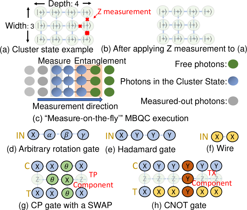
Figure 1. Cluster state and Measurement pattern examples.

2. Background

Measurement-based quantum computing (MBQC) carries out the computation on a 2-D mesh of entangled photon qubits, which is referred to as a cluster state. A cluster state consists of photon qubits initially prepared in the $\ket{+}$ state where each photon is entangled with its neighboring photons. Fig. 1(a) illustrates a photonic cluster state with 12 photons. We next elaborate on the details of photonic cluster states (Section 2.1) and MBQC on cluster states (Section 2.2).

2.1. Photonic Cluster State

A cluster state is generated by a photonic hardware generator (i.e., cluster state generator) that continuously produces entangled photons (coupleemitter1, ; coupleemitter2, ; coupleemitter3, ; pichler2017universal, ; 24row, ; 2023deterministic, ; quantumdot, ). Fig. 1(c) shows such a generation process in which the generator has a fixed width of 3 photons and the entangled photons are generated from left to right. In the 2-D mesh cluster state, the width and depth are important for a quantum circuit execution on a cluster state (mbqccluster, ; dac, ; introduction, ).

Cluster state width. The width refers to the number of rows in a cluster state. A fixed width simplifies photonic cluster state generator hardware, which is a typical design (coupleemitter1, ; coupleemitter2, ; coupleemitter3, ; pichler2017universal, ; 2023deterministic, ; 24row, ). However, the minimum width required by each quantum algorithm varies according to the number of logical qubits it has (mbqccluster, ; dac, ; mbqc, ). Specifically, each logical qubit is mapped to a row of photons in the cluster state. To prevent undesired interactions between two logical qubits, the corresponding photon rows cannot be adjacent since the adjacent photons are entangled in a cluster state. Therefore, MBQC cuts out one row of photons between the two rows where logical qubits are mapped. Hence, a quantum algorithm requires a minimum of $2N_{q}-1$ rows to be executed in a cluster state, where $N_{q}$ represents the number of qubits in the quantum algorithm (mbqccluster, ; fly, ; dac, ).

Cluster state depth. The depth refers to the number of columns in a cluster state. A hardware generator produces entangled photons from left to right, where there are no hardware generator constraints in the cluster state depth. Thus, the depth of the cluster state is only determined by a quantum algorithm and its mapping on the cluster state. The depth is necessary to reduce execution time: the shorter the cluster state depth, the faster the execution and the lower the error rate (coupleemitter1, ; coupleemitter2, ; coupleemitter3, ; pichler2017universal, ; 2023deterministic, ; quantumdot, ; photonicreview, ). Therefore, our goal is to reduce the depth in a fixed-width cluster state to execute a quantum algorithm.

Fig. 1(c) also illustrates the “measure-on-the-fly” execution paradigm employed in the cluster state (fly, ; photonicreview, ; optical, ). That is, the measurements are applied to the photons while the cluster state is generated. This avoids the need to store a large-scale photonic cluster state in optical quantum memory, increasing MBQC’s scalability (fly, ; photonicreview, ; optical, ). Note that the measurement direction must be the same as the cluster state generating direction in this paradigm (i.e., from left to right). As shown in Fig. 1(c), the cluster state generator entangles free photons (green circles) into a cluster state (blue circles). Meanwhile, a column of photon detectors measures the leftmost column of the cluster state to perform computations. Once measured, the photons (gray circles) are no longer entangled.

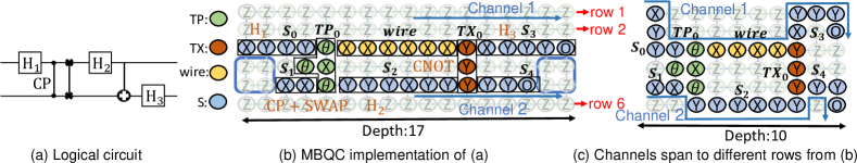
Figure 2. Example of a quantum algorithm mapped on a cluster state.

2.2. MBQC on Cluster State

MBQC employs two types of measurements to achieve universal quantum computation (oneway, ; mbqccluster, ): i) X and Y measurements ($\sigma_{x}$ and $\sigma_{y}$ eigenbasis) to perform Pauli gate operations (oneway, ; mbqccluster, ), and ii) $\theta$ measurements to perform non-Pauli gate operations. Implementation of quantum gates (also called “pattern” (mbqccluster, )) is achieved by a set of measurements applied to entangled photons in cluster states. Fig. 1 shows several pattern examples with annotated measurement angles. The patterns of a single-qubit arbitrary rotation gate and an H gate are shown in Fig. 1(d) and (e), where measurements are applied to a row of consecutive entangled photons and computation is carried out “one-way” from left to right. The consecutive X measurements of even numbers serve as identity gates or “wires”, allowing logical qubit transmission through qubit rows without applying any quantum operations (mbqccluster, ) (Fig. 1(f)).

MBQC uses Z measurements to “cut out” entangled photons from a cluster state (oneway, ; mbqccluster, ). Fig. 1(a) shows an example of applying a Z measurement to a photon in the cluster state, destroying the entanglements between the photon and its neighbors. The resulting cluster state is shown in Fig. 1(b). The Z measurements eliminate unwanted interactions between logical qubits by separating qubit rows in a cluster state. It also eliminates any photons within the cluster state that are not involved in the computation.

Two notable two-qubit gate patterns are the combined CP and SWAP gate and the CNOT gate, shown in Fig. 1(g) and (h), where measurements are applied to three rows of entangled photons. The first row corresponds to the control qubit, whereas the third row corresponds to the target qubit. Among the measurements in the middle row, the X, $\theta$, and Y measurements facilitate communication between the two logical qubits, while the Z measurements cut out unused photons and separate rows for control and target qubits. While CNOT and single-qubit gates together enable universal quantum computation (universality, ; nielsen2001quantum, ), MBQC provides further advantages as CNOT gates together with combined CP and SWAP gates reduce the need for quantum gate decomposition and enhance the flexibility of quantum computation (mbqccluster, ).

3. Opportunities and Challenges

We use a real MBQC example to illustrate the opportunities and challenges in optimizing the cluster state depth. Fig. 2(a) shows a two-qubit quantum algorithm, where its corresponding MBQC implementation on a photonic cluster state is shown in Fig. 2(b). After the computation on a logical qubit (i.e., a photon row), an output photon is employed for readout measurement $O$. Fig. 2(b) shows the mapping from a quantum algorithm to a cluster state, which we refer to as an MBQC circuit in the rest of this paper.

The one-way computation in MBQC can result in long cluster state depth, which is often due to inefficient photon usage. For example, only three of six photon rows are being used in Fig. 2(b). That is, rows 1, 2, and 6 in Fig. 2(b) are not used by effective computation and are cut out by Z measurements. Moreover, there are Z measurements that cut out photons within the three used photon rows, as indicated by the blue boxes. This motivates the question: Can we leverage these unused photons and rows to reduce the circuit depth?

3.1. MBQC Circuit Variants

In practice, the measurements corresponding to a logical qubit in a cluster state are not necessarily mapped to the same row. This is because the quantum computation on a logical qubit remains unchanged as long as the same measurements are made on entangled photons in the same order as in a cluster state (oneway, ; mbqccluster, ). That is, one can leverage the entangled photons in the same column, rather than being strictly limited to entangled photons in the same row. We define the measurement sequences on entangled photons in cluster states as “channels”. Note that measurements within a column can be performed either simultaneously or sequentially (photonicreview, ; optical, ). In the baseline MBQC circuit mapping, one channel is necessarily mapped to one photon row. However, if we allow the channel to span multiple rows, it can leverage unused photons and potentially reduce depth.

Different MBQC circuits can be generated when the channel spans multiple photon rows in a cluster state. To explore shorter MBQC circuits with the same function, we first partition an MBQC circuit into different components, then explore the variant of each component and connect them together. Each component is a group of adjacent measurements with a specific functionality. We define four types of components:

• TP: The TP component is used to connect the control qubit (i.e., control channel) and the target qubit (i.e., target channel) in the combined CP and SWAP gate pattern. It consists of one X and three $\theta$ measurements. The four measurements of a TP component are colored in green in Fig. 1(g).

• TX: The TX component consists of three Y measurements and is used to connect the control qubit and the target qubit in CNOT gate patterns. The TX component is colored in red in Fig. 1(h). The three Y measurements in the TX component are required to be measured simultaneously (mbqccluster, ).

• S: The S component represents single-qubit measurements. An S component consists of consecutive measurements within individual channels, e.g., Fig. 1(d) and Fig. 1(e). Note that an S component cannot include pairs of X measurements because they only form wires.

• wire: A wire is a consecutive sequence of an even number of X measurements. As previously discussed, a wire only serves as a connector between two components and does not perform any quantum computation.

Based on these four types of components, we next define intra-component variants and inter-component variants.

Intra-component variants: For each component, there are multiple MBQC mappings that have the same quantum functionality as in a baseline MBQC circuit. Specifically, each type of component has its own unique set of variants:

• TP variants: A TP component has only one valid variant. Fig. 3(a) shows the TP component in the baseline MBQC circuit, whereas Fig. 3(b) shows its valid variant and one example of an invalid variant. The valid variant swaps the $\theta_{0}$ and $\theta_{2}$ measurements in the first and third rows, respectively. As discussed in Section 2.1, the measurements in a cluster state are performed from left to right. This implies that measurements in the first column should be executed before those in the second column. As such, the valid variant preserves the same order as the baseline because the same measurements are present in each column. In contrast, the invalid variant does not preserve the same measurement order, resulting in an incorrect computation due to a different measurement sequence (oneway, ; mbqccluster, ).

• TX variants: Similar to the TP component, the TX component also has only one valid variant. Fig. 3(c) shows the baseline TX component and Fig. 3(d) shows its valid variant and one example of an invalid variant. The valid TX variant also swaps the baseline TP component measurements. In both the baseline TX component and the valid TX variant, the three Y measurements can be performed simultaneously as they are in the same photon column. However, in the invalid variant, Y₂ and Y₃ are measured after Y₁, leading to incorrect computation.

• S variants: Fig. 3(e) shows an example of an S component with three measurements. In the baseline S component, measurements follow a left-to-right sequence, from X to Y₁. Although the two Y measurements are in the same column in the valid variant shown in Fig. 3(f), X is measured first in the left column and Y₀ can be measured before Y₁ (photonicreview, ; optical, ). Hence, the same measurement order can still be kept. In contrast, in the invalid variant, the X measurement is to the right of the two Y measurements and it would be measured after these two.

• wire variants: A wire component only requires an even number of X measurements. Fig. 3(g) shows three variants of a wire component. The valid variant I has six X measurements and the valid variant II has two. The invalid variant has one measurement, changing the wire’s function.

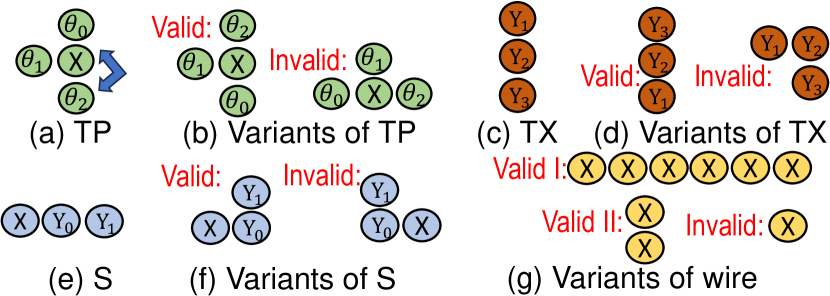
Figure 3. Intra-component variants.

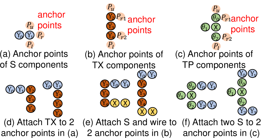
Figure 4. Anchor points in components.

Inter-component variants: Between two adjacent components, we refer to the component on the left as the “left component” and the component on the right as the “right component,” and refer to measurements linking these adjacent components as “connected points.” By adjusting the positions between two adjacent components, we can decrease the depth of an MBQC circuit by optimizing photon use in a cluster state. In this process, it is essential to maintain the connection between adjacent components, where the right component’s connected point should attach to the “anchor points” on the left component. Anchor points are defined as the unused neighboring photons of the left component’s connected point, where the right components can be attached. For example, Fig. 4(a) shows the three anchor points of the S component ($P=\{P_{u},P_{r},P_{l}\}$). Applying the TX component to $P_{u}$ is not possible as it results in overlapping measurements, which is not allowed in MBQC (mbqccluster, ). As shown in Fig. 4(d), anchoring at $P_{l}$ reduces circuit depth compared to $P_{r}$. Unlike the S component, TP and TX components offer two anchor points, as shown in Fig. 4(b) and (c). In Fig. 4(e) and (f), each right component of the TP and TX components applies to a different pair of anchor points, where the pair $(P_{u},P_{l})$ minimizes circuit depth.

Illustrating intra- and inter-component opportunities: Exploiting both intra-component and inter-component variants allows us to reduce the circuit depth while maintaining the correct quantum function. An example is shown in Fig. 2(c) which is functionally equivalent to the MBQC circuit in Fig. 2(b). Specifically, for intra-component, we use variants of S₀, S₃, and S₄ that span more rows to reduce the depth. For inter-component, we attach S₂ to the lower anchor point of TP₀, attach TX₀ to the upper anchor point of S₂, and attach S₃ to the upper anchor point of TX₀. As a result, the depth is reduced from 17 (in Fig. 2(b)) to 10 (in Fig. 2(c)) by leveraging both variants.

3.2. MBQC Constraints

While exploiting intra- and inter-component variants allows us to reduce the depth, it is a nontrivial task where certain constraints have to be satisfied to guarantee correctness.

Constraint-I Channel connectivity. It is crucial to ensure channel connectivity in the MBQC circuit. That is, the sequence of measurements (i.e. the channel) should remain the same as in the baseline circuit. This constraint is violated if a channel is disconnected between two adjacent measurements. In Fig. 5(a), we show an S component adjacent to a TX component. Fig. 5(b) shows this constraint violation due to a disconnected channel.

Constraint-II Invalid connection. Measurements that have no connection in the baseline MBQC circuit should remain disconnected. This violation occurs when using an inappropriate variant or connecting components to inappropriate anchor points. For instance, in example I of Fig. 5(c), an invalid connection, marked by the red cross, is caused by the adoption of an inappropriate variant of the S component where the Y₀ and Y₃ measurements are connected. In example II of Fig. 5(c), there is an invalid connection between X and Y₂ due to the inappropriate anchor points.

Constraint-III Component dependency. The dependency among the components has to be maintained when exploring MBQC circuit variants to ensure quantum computation correctness. That is, any component (including all the measurements in it) should not be conducted before those components it depends on.

Constraint-IV Cluster state width. The depth-reduced MBQC circuit must not have variants that exceed the fixed width of the cluster state. Violating this constraint makes the quantum circuit inexecutable on the cluster state (mbqccluster, ; dac, ; mbqc, ).

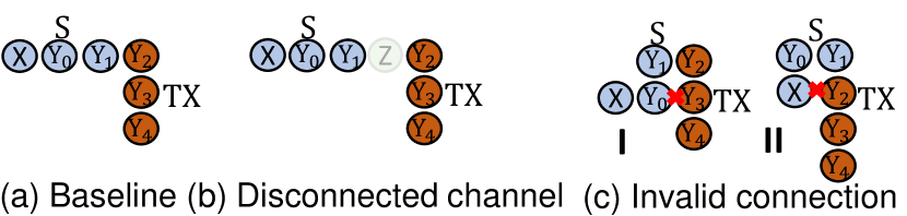
Figure 5. Examples of violating constraints.

4. Our Approach

In this paper, we design FMCC (Flexible MBQC Compilation on Cluster State), an MBQC compilation framework that exploits both intra-component and inter-component variants while satisfying the aforementioned constraints. However, this process faces two challenges. First, the design space can be prohibitively large, making exhaustive search practically infeasible. For instance, given a circuit with $n$ components, if each component has $v$ variants and $k$ anchor points, conceptually, one can have $v^{n}\times k^{n-1}$ MBQC circuits. While a simple heuristic may work, the second challenge is that among the $v^{n}\times k^{n-1}$ MBQC circuits, many of them may be invalid due to constraints violations. As such, a heuristic approach may lead to invalid MBQC circuits. To this end, our proposed FMCC employs dynamic programming (DP) to construct a valid MBQC circuit with reduced depth, while addressing the two challenges.

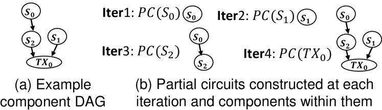
Figure 6. Partial circuit set constructed at each iteration.

4.1. Constructing MBQC Circuits

In FMCC, MBQC circuits are built component-wise. The construction sequence is guided by a Directed Acyclic Graph (DAG), which captures the dependencies among non-wire components, referred to as a component DAG. We iterate through each component of the DAG, to generate a set of variants for that component. In each iteration, one component is chosen from the DAG. We define a variant set for a component chosen at iteration $k$ as:

Definition 1.

(Variant set) The variant set $V(c)$ at iteration $k$ is the set of all valid variants of the component $c$ selected at iteration $k$, including its baseline variant.

Starting from the independent components, i.e., components without parents in the DAG, a set of partial circuits is constructed iteratively by integrating the set of variants for the selected component. We define the partial circuit set as:

Definition 2.

(Partial circuit set) The set of partial circuits $PC(c_{i})$ for the selected component $c_{i},$ where $i\in\{1,...,n\}$ for $n$ components in the DAG, has elements constructed using the set of partial circuits for $c_{i-1}$ (i.e., $PC(c_{i-1})$) with the variant set of $c_{i}$ (i.e., $V(c_{i})$), where $c_{i-1}$ is the parent component of component $c_{i}$ in the DAG. That is,

(1) $$PC(c_{i})=\cup_{z\in P}(PC_{x}\oplus V_{y})$$

$$\forall\ PC_{x}\in PC(c_{i-1}),\ and\ \forall\ V_{y}\ \in\ V(c_{i})$$

where $PC_{x}$ is a partial circuit in $PC(c_{i-1})$, $V_{y}$ is a variant of component $c_{i}$ in $V(c_{i})$, $\oplus$ stands for both component integration and partial circuit combination, and $P$ is the set of all anchor points in $PC_{x}$.

To illustrate the partial circuit set constructed in each iteration, consider the component DAG in Fig. 6(a) which includes $n=4$ components. In the first iteration, the independent component S₀ is selected and all its valid variants are generated as $V(S_{0})$. Since S₀ lacks parent components, partial circuit set $PC(S_{0})$ is generated using the initial partial circuit set $\emptyset$ and $V(S_{0})$. Similarly, in the second iteration, $PC(S_{1})$ is generated using $\emptyset$ and $V(S_{1})$. In the third iteration, $PC(S_{2})$ is generated by integrating $PC(S_{0})$ and $V(S_{2})$ since S₂ has a parent component S₀ in the DAG. In the fourth iteration, $PC(TX_{0})$ is generated by integrating $PC(S_{2})$, $PC(S_{1})$, and $V(TX_{0})$ according to Equation 1.

With the definitions of variant and partial circuits, we next elaborate on how FMCC constructs an MBQC circuit. At each iteration, one independent component is selected and removed from the component DAG. Based on the position of the component in the DAG, FMCC performs either component integration or partial circuit combination. Following this, wires may be inserted.

Component integration. At the beginning, FMCC starts with the initial partial circuit set as $\emptyset$ and selects the first independent component from the DAG. If there are multiple independent components, FMCC randomly chooses one of them. Fig. 7(a) shows an example DAG with two components S₀ and TX₀. Since S₀ is independent, FMCC chooses S₀ as the first component. Next, FMCC generates the variant set of S₀, i.e. $V(S_{0})$, which contains all the variants of S₀, as shown in Fig. 7(b). Based on equation 1, the partial circuit set $PC(S_{0})$ is constructed by adding $V(S_{0})$ to $\emptyset$, the initial partial circuit set. Next, TX₀ becomes independent as S₀ is removed from the DAG in the previous iteration. FMCC chooses TX₀ and generates its variants set $V(TX_{0})$ as shown in Fig. 7(c). Then, FMCC performs component integration using the partial circuit set $PC(S_{0})$ and the variants set $V(TX_{0})$. According to equation 1, all the anchor points of each partial circuit $PC_{x}$ in $PC(S_{0})$ are explored with each variant $V_{y}$ in $V(TX_{0})$. Take as an example the 5th partial circuit ($PC(S_{0})_{5}$ in Fig. 7(b)) and the 2nd variant of TX₀, Fig. 7(b) shows the three anchor points ($P=\{P_{u},P_{r},P_{l}\}$) of $PC_{5}$. FMCC integrates the TX₀ variants to each of the anchor points, generating partial circuits shown in Fig. 7(d). This results in the first three variants being valid, while the fourth has an invalid connection. FMCC constructs the partial circuit $PC(TX_{0})$ by exploring all the partial circuits in $PC(S_{0})$ and all the variants in $V(TX_{0})$.

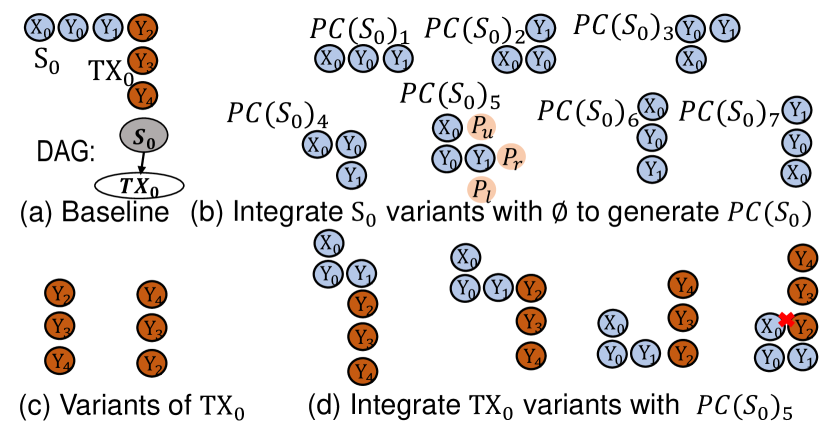
Figure 7. Example of component integration.

Partial circuit combination. Selected components can have more than one parent, which additionally requires combination. For example, in Fig. 8(a), TX₀ has two parent components (S₀ and S₁). In this case, partial circuit combination of the two dependent sets $PC(S_{0})$ and $PC(S_{1})$ is required before TX₀ can be integrated. The combination follows an all-to-all manner. That is, each partial circuit from $PC(S_{0})$ is combined with each partial circuit from $PC(S_{1})$ in combination. Fig. 8(b) illustrates this using $PC(S_{0})_{5}$ from $PC(S_{0})$, the only partial circuit $PC(S_{1})_{0}$ in $PC(S_{1})$, and the first variant of TX₀ to generate four new partial circuits by exploring the anchor points $P=\{(P_{r}^{Y_{1}},P_{r}^{X1}),(P_{l}^{Y_{1}},P_{r}^{X1}),(P_{r}^{Y_{1}},P_{u}^{X1}),(P_{l}^{Y_{1}},P_{u}^{X1})\}$. Note that other anchor point combinations in $PC(S_{0})_{5}$ and $PC(S_{1})_{0}$ are not possible. Consequently, $PC(TX_{0})$ is formed by combining the two sets of partial circuits and integrating the selected component while exploring all the anchor points.

Wire insertion. As discussed in Section 2.1, the function of a wire component is to connect a dependent component to its parent. Also, recall from Section 3.1, a wire can have valid variants with different even numbers X measurements. FMCC inserts wires on demand with appropriate wire variants to connect the dependent components whenever necessary. For example, Fig. 9(a) shows a baseline MBQC circuit. Consider a valid partial circuit generated from the previous iteration in Fig. 9(b). FMCC inserts a wire (two X measurements) to connect TX₁ to its parent S₁.

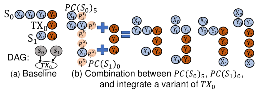
Figure 8. Example of partial circuits combination.

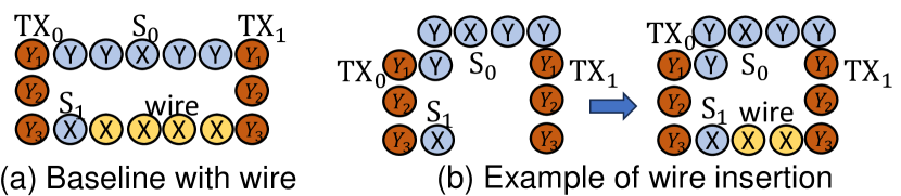
Figure 9. Example of wire insertion.

4.2. Partial Circuits Pruning

The partial circuit construction involves exploring all the variants and all the anchor points. It is difficult to track of all the partial circuits as the design space increases exponentially with the number of components. Fortunately, many of the partial circuits are invalid due to violation of the constraints (Section 3.2), such as the example in Fig. 7(d) where there exists an invalid connection between X₀ and Y₂. FMCC drops all the invalid partial circuits. However, FMCC may still generate so many valid partial circuits that it is impractical to track them all. Therefore, to reduce the design space, FMCC employs a threshold $m$ to prune the set of partial circuits in each iteration. Specifically, for a partial circuit set $PC(c)$, we divide it into multiple sets where each set contains the partial circuits with the same width (i.e., $PC(c)=PC(c)^{w_{1}}\cup PC(c)^{w_{2}}\cup\cdots\cup PC(c)^{w_{q}}$, where $w_{1}$, $w_{2}$, $\cdots$, $w_{q}$ are the partial circuit width). For the partial circuit set of each width $PC(c)^{w_{i}}$, we retain the top $m$ partial circuits and drop the others to reduce the size of $PC(c)$. We choose different widths because it is more likely to produce a valid MBQC circuit with reduced depth. As discussed in Section 3, an MBQC circuit can reduce its depth by using more photon rows. Similarly, the depth of a partial circuit can be decreased by utilizing more rows (wider width). However, keeping only the partial circuits with a larger width may lead to an MBQC circuit width that exceeds the cluster state width after a combination. On the other hand, retaining partial circuits with a smaller width reduces this risk but may result in a deeper MBQC circuit. As a result, we retain $m$ partial circuits in $PC(c)^{w_{i}}$ for each width ${w_{i}}$ to achieve a valid and shorter MBQC circuit.

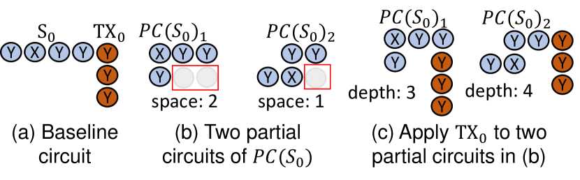
Figure 10. Example of leveraging space.

We next answer the question: which $m$ partial circuits to retain? We leverage two metrics: i) depth and ii) space. Since the circuit depth is the objective of FMCC, a partial circuit with a shorter depth is preferred as it is more likely to generate a shorter MBQC circuit. If multiple partial circuits have the same width and depth, we use space to determine which $m$ partial circuits to retain. Particularly, space is defined as the number of unused photons after each rightmost measurement in a partial circuit. For example, Fig. 10(a) shows a circuit with two components S₀ and TX₀. The space is annotated in Fig. 10(b) for two partial circuits of $PC(S_{0})$. The unused photons in the space may be used by component integration in the next iteration. Therefore, a larger space indicates a larger potential to generate short depth when integrating the next component. To illustrate this, consider the example in Fig. 10(c). If we choose the $PC(S_{0})_{1}$ which has 2 spaces, we can generate the partial circuit with depth 3 after integrating TX₀. In contrast, if we choose $PC(S_{0})_{2}$, which has 1 space, we will have the partial circuit with depth 4 after integrating TX₀. In FMCC, the width, depth, and space are tracked using a table where each row of the table is a partial circuit.

Algorithm 1 FMCC

0:  Component DAG $G$, a cluster state $CS$, $m$

0:  Minimized-depth MBQC circuit Initialization: Partial circuits sets $PC$ = []

1:  while $G$ != [] do

2:     $c=independent(G)$

3:     $G.remove(c)$

4:     $V(c)=Generate\_variants(c)$

5:     $c_{parent1},c_{parent2}=Find\_parent(c)$

6:     $PC(c)$ = []

7:     for $V_{y}$ in $V(c)$ do

8:        if $c_{parent2}==\emptyset$ then

9:           for $PC_{x}$ in $PC(c_{parent1})$ do

10:              $P=Find\_Anchor\_Points(PC_{x})$

11:              for $P_{1}$ in $P$ do

12:                 $PC(c)_{x}=integrate(V_{y},PC_{x},P_{1})$

13:                 $PC(c)_{x}=insert\_wire(PC(c)_{x})$

14:                 $PC(c).append(valid(PC(c)_{x}))$

15:        else if $C_{parent2}!=\emptyset$ then

16:           for $PC_{x1}$ in $PC(c_{parent1})$ do

17:              for $PC_{x2}$ in $PC(c_{parent2})$ do

18:                 $P^{c_{parent1}}=Find\_Anchor\_Points(PC_{x1})$

19:                 $P^{c_{parent2}}=Find\_Anchor\_Points(PC_{x2})$

20:                 for $P_{1}$ in $P^{c_{parent1}}$ do

21:                    for $P_{2}$ in $P^{c_{parent2}}$ do

22:                       $PC(c)_{x}=combine(V_{y},PC_{x1},PC_{X2},P_{1},P_{2})$

23:                       $PC(c)_{x}=insert\_wire(PC(c)_{x})$

24:                       $PC(c).append(valid(PC(c)_{x}))$

25:     $Table=create\_table(PC(c))$

26:     $PC=PC+select\_top\_m(PC(c),Table,m,CS))$

27:  return  $shortest(PC[-1])$

4.3. Detailed Algorithm of FMCC

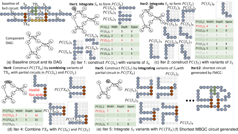
Figure 11. Example of FMCC Constructing circuit variant.

The detailed algorithm of FMCC is shown in Algorithm 1. The input is the component DAG $G$, a cluster state, and the parameter $m$ for retaining partial circuits. The output is the MBQC circuit with minimal depth. In each iteration, FMCC selects and removes an independent component $c$ from the component DAG (lines 2-3). FMCC then generates all its variants as a variant set $V(c)$ (line 4) and identifies its parent components (line 5). If $c$ has less than two parent components, FMCC conducts component integration that integrates each variant from $V(c)$ with each partial circuit $PC_{x}$ in $PC(c_{parent1})$ where $c_{parent1}$ is the parent component of $c$, while considering all anchor points $P$ (lines 8-14). When $c$ has two parent components, FMCC performs partial circuit combination of $PC(c_{parent1})$ and $PC(c_{parent2})$, and then integrates variants in $V(c)$ while exploring all the anchor points (lines 15-24). In this process, for each $PC(c)_{x}$ in $PC(c)$, FMCC inserts a wire if necessary (lines 13 and 23) and removes invalid $PC(c)_{x}$ (lines 14 and 24). Also, FMCC maintains a table to record the width, depth, and space for each partial circuit $PC(c)_{x}$ in $PC(c)$ (line 25), and uses the table to retain the $m$ partial circuits with the same width (line 26).

4.4. A Walk-Through Example

We now go through a real benchmark (i.e., 3-qubit Bernstein–Vazirani — bv3) to illustrate the steps of FMCC in Fig. 11. The baseline MBQC circuit of bv3 and its component DAG are shown in Fig. 11(a). Let us assume that the cluster state width $w$ is 8 and the retained partial circuit count $m$ is 2. There are a total of 12 iterations due to 12 non-wire components in the DAG. Due to the lack of space, Fig. 11 only shows five iterations, which are sufficient to illustrate the steps of FMCC. In each iteration, we plot the table of the width, depth, and space of each partial circuit. We also highlight the chosen component in each iteration and show the remaining components in the DAG. For each partial circuit, photons contributing to space are indicated with gray-shaded circles.

Initially, there are three independent components: S₆, S₂, and S₀. Thus, in the first three iterations, FMCC conducts the component integration for each independent component and generates $PC(S_{6})$, $PC(S_{2})$, and $PC(S_{0})$. Fig. 11(b) shows the first iteration where S₆ is selected to construct $PC(S_{6})$. There are more than 30 variants of S₆ and we show representative seven of them in Fig. 11(b), labeled from $PC(S_{6})_{1}$ to $PC(S_{6})_{7}$. Among the seven partial circuits, one has a width of 1, three have a width of 2, and three have a width of 3. Since $m$ is 2, FMCC will retain the only variant with width 1, two out of three variants with width 2, and two out of three variants with width 3. For $PC(S_{6})_{2}$, $PC(S_{6})_{3}$, and $PC(S_{6})_{4}$ that have the same width 2, they also have the same depth. Therefore, the two with large spaces are retained, and the one with smaller space ($PC(S_{6})_{4}$) is pruned (shaded in the table). Similarly, For $PC(S_{6})_{5}$, $PC(S_{6})_{6}$, and $PC(S_{6})_{7}$ that have the same width of 3, they also have the same depth. $PC(S_{6})_{7}$ is pruned as it has the smallest space. In iteration 2, the procedure is similar. We show eight representative partial circuits of $PC(S_{2})$ ($PC(S_{2})_{1}$ to $PC(S_{2})_{8}$) in Fig. 11(c). Among the eight partial circuits, $PC(S_{2})_{1}$ to $PC(S_{2})_{4}$ have the same width of 4 and the same depth of 4. $PC(S_{2})_{3}$ and $PC(S_{2})_{4}$ are pruned due to their smaller space. Similarly, $PC(S_{2})_{5}$ to $PC(S_{2})_{8}$ have the same width of 5 and the same depth of 3. $PC(S_{2})_{7}$ and $PC(S_{2})_{8}$ are pruned. In iteration 3, FMCC performs the same procedure to construct $PC(S_{0})$.

In iteration 4, TX₀ is independent and selected. Since TX₀’s parent components are in two partial circuit sets $PC(S_{6})$ and $PC(S_{2})$, FMCC performs combination of $PC(S_{6})$ and $PC(S_{2})$, and integrates $V(TX_{0})$ with the combined partial circuits. We plot four example partial circuits generated after TX₀ integration in Fig. 11(d). The first one has a width of 9 which is larger than the fixed cluster state width of 8. Therefore, FMCC prunes it from $PC(TX_{0})$. The other three partial circuits $PC(TX_{0})_{1}$, $PC(TX_{0})_{2}$, and $PC(TX_{0})_{3}$ have the same width of 7. Since $PC(TX_{0})_{1}$ and $PC(TX_{0})_{2}$ have a shorter depth (5) compared to $PC(TX_{0})_{3}$’s depth (6), they are retained in $PC(TX_{0})$, and $PC(TX_{0})_{3}$ is pruned.

In iteration 5, S₃ becomes independent and $V(S_{3})$ is integrated with the partial circuits in $PC(TX_{0})$. We show four generated partial circuits with the same width in Fig. 11(e). $PC(S_{3})_{1}$ and $PC(S_{3})_{4}$ are kept due to their shorter depth of 5. For the remaining iterations, similar integration and combination processes are conducted by FMCC to generate sets of partial circuits. Fig. 11(f) shows the MBQC circuit with the minimized depth after iteration 12.

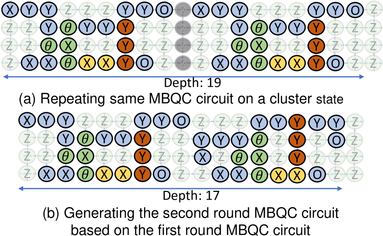
Figure 12. Executing two rounds of MBQC circuits.

4.5. Optimizing Multiple Rounds

The same quantum circuit usually executes multiple times to obtain stabilized output distribution (nielsen2001quantum, ). This equivalently maps to the same MBQC circuits executing multiple times, which we referred to as “rounds”. Fig. 12(a) shows a quantum circuit that executes two rounds on a cluster state. As one can observe, a column of photons is cut out to separate the two rounds, annotated by gray photons, which extends the overall circuit depth. Fortunately, our proposed FMCC can be seamlessly applied to consecutive rounds of a quantum circuit. Specifically, for MBQC circuits with the same width of a round, FMCC keeps track of the top $m$ for that round and applies the same procedure (discussed in Section 4.1 and Section 4.2) when picking up the components from the next round. This allows us to utilize the cut-out photons at the end of each MBQC round. For instance, Fig. 12(b) shows a valid two-round execution where the second round does not have any connection with the first round, but is able to utilize the cut-out photons and reduce the depth to 17. It is also to be noted that, the second round has a different valid MBQC circuit compared to the first round.

5. Evaluation

5.1. Experiment Setup

Benchmarks and Metric: We use five representative quantum applications (shown in Table 1) to evaluate FMCC: Quantum Fourier Transform (qft) (qft, ), hardware efficient ansatz (hwea) (hwea, ), Bernstein–Vazirani (bv) (bv, ), instantaneous quantum polynomial time (iqp) (iqp, ), and linear hydrogen atom chain (hc) (hc, ). For each application, we evaluate three different numbers of qubits: 5 qubits (small), 15 qubits (medium), and 27 qubits (large). Note that, hc requires an even number of qubits (hc, ). Therefore, we use 6, 14, and 26 qubits as the small, medium, and large for hc, respectively. We use the cluster state depth reduction ratio as the metric to measure the effectiveness of our approach.

Baseline: The baseline employs the state-of-the-art MBQC compilation on photonic cluster state (dac, ). This baseline optimizes the depth of the MBQC circuit by leveraging independent gate reordering, redundant wire removal, and consecutive single-qubit gate combinations. We use this baseline to demonstrate the significant depth reduction brought by FMCC over the state-of-the-art.

Fixed cluster state width: As discussed in Section 2.2, the minimum cluster state width for a $N_{q}$-qubit benchmark is $2N_{q}-1$. We use two different fixed cluster state widths to evaluate FMCC: i) $1.25\times(2N_{q}-1)$, referred to as C1, and ii) $1.5\times(2N_{q}-1)$, referred to as C2.

As discussed in Section 4.2, FMCC keeps track of the $m$ partial circuits for each width. For the main results, we empirically choose $m$ to 12, which we find is enough to provide the minimized depth. We also conduct a sensitivity study of different $m$ values in Section 5.5.

Appli-	small			medium			large
cation	qubit	C1	C2	qubit	C1	c2	qubit	C1	C2
bv	5	12	14	15	37	44	27	67	80
iqp	5	12	14	15	37	44	27	67	80
hwea	5	12	14	15	37	44	27	67	80
qft	5	12	14	15	37	44	27	67	80
hc	6	14	17	14	34	41	26	64	77

Table 1. Number of qubits and width for each benchmark.

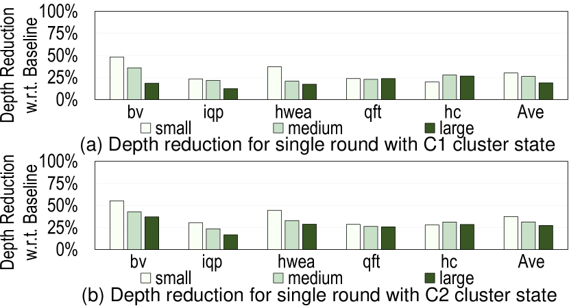
Figure 13. Depth reduction for single round.

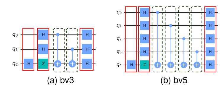
Figure 14. Different qubit number bv and the gate layers.

5.2. Single Round Results

We show the depth reduction ratios achieved by FMCC of a single round in Fig. 13 and multiple rounds (i.e., 100 rounds) in Fig. 15. Fig. 13 and Fig. 15 also contain results under different fixed cluster widths (i.e., C1 and C2). As shown in Fig. 13(a), FMCC achieves an average of 30.2%, 26.2%, and 19.0% depth reductions for small, medium, and large under C1 cluster state width, respectively. Similarly, under C2 width, FMCC achieves an average of 37.3%, 31.3%, and 27.0% depth reductions, respectively. For all three numbers of qubits, the reductions increase from C1 to C2, indicating that FMCC effectively leverages the redundant photons rows in wider cluster states to reduce the depth.

The depth reduction ratio decreases with more number of qubits for bv, iqp, and hwea. To illustrate the reason, let us consider 3-qubit bv in Fig. 14(a) and 5-qubit bv in Fig. 14(b). In the figure, we annotate the layers of the single-qubit gate using red boxes and the layers of the two-qubit gate using green dash boxes. A layer is a collection of independent gates that can be performed concurrently. As one can observe, the number of two-qubit gate layers increases with the number of qubits. As such, there are more dependent TX components in the component DAG. For instance, Fig. 14(a) has two layers of two-qubit gates, and Fig. 14(b) has four layers of two-qubit gates. Recall that in Section 3, the TX and TP components have fewer variants and less reduction in depth compared to the S components. Therefore, with more TX components in large qubit counts, the depth reduction brought by FMCC also decreases. Similar results exist in the iqp and hwea, where with a larger qubit size, iqp has more TP components and hwea has more TX components.

In the hc, the depth reduction increases from small to medium qubit count, and then decreases from medium to large qubit count. This is because hc has long S components where many of its variants are invalid in the small qubit count since it exceeds the fixed cluster state width (14 in C1 and 17 in C2). In the medium qubit count, the cluster state is wider, so more valid S components can be accommodated. However, in the large qubit count, the depth reduction decreases because hc also has an increased number of two-qubit gate layers as bv, iqp, and hwea. qft exhibit similar depth reduction in all qubit counts. This is because the number of S components is proportionally increased with more qubits, providing a constant potential for depth reduction.

5.3. Multiple Round Results

We evaluate one hundred rounds of each benchmark in Fig. 15. As one can observe, for C1, FMCC achieves average of 42.7%, 49.0%, and 47.5% depth reductions for small, medium, and large, respectively. The depth reductions are 53.5%, 60.6%, and 60.0% on C2. Compared to the single-round results in Fig. 13, FMCC achieves higher depth reduction, indicating its effectiveness in utilizing the cut-out photons between consecutive rounds as we discussed in Section 4.5.

For the bv, qft, and hc, the trend of depth reduction across the three qubit counts is similar to the trend observed in the single round results (Fig. 13), indicating that FMCC effectively exploits both single round depth reduction and multi-round depth reduction. However, iqp and hwea are two exceptions. For iqp, the depth reduction increases from small to medium qubit count due to the effectiveness of FMCC multi-round optimization. However, the depth reduction drops from medium to large qubit count due to the increasing number of two-qubit gate layers (the same as the iqp single round case). In contrast, the depth reduction of hwea increases with more qubits. This is because with more number of qubits, the cut-out photons at the end of a hwea round (i.e., after the last component in a round is integrated) increases. Recall our discussion in Section 4.5 where the cut-out photons can be leveraged by consecutive rounds. Therefore, with more cut-out photons in the large qubit count, the depth reduction is also larger.

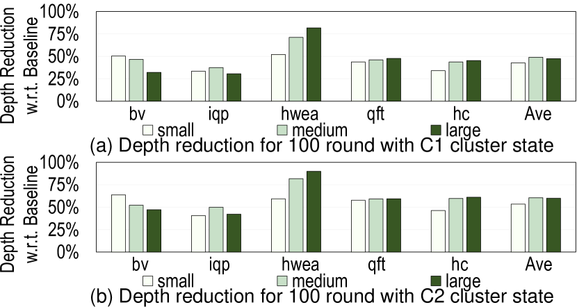
Figure 15. Depth reduction for 100 rounds.

5.4. Photon Utilization

We plot the photon utilization of the single round in Fig. 16 and the multi-round in Fig. 17. Photon utilization is defined as the ratio of non-z measurements in a cluster state to all the number of measurements in the cluster state. FMCC yields significant improvement in photon utilization compared to the baseline. On average, FMCC achieves the photon utilization of 37.3%, 33.5%, 50.1%, and 51.8% in single round C1, C2, and multi-round C1, C2, respectively. This is significantly higher compared to the baseline (27.0%, 22.0%, 27.0%, and 22.0% in single-round C1, C2, and multi-round C1, C2, respectively), indicating that FMCC effectively exploits the cutout photons to reduce the MBQC circuit depth.

5.5. Sensitivity Study

Large number of qubits. We evaluate bv and qft using 50 and 100 qubits to study the scalability of FMCC using C2 fixed cluster state width (i.e., 149 rows for 50 qubits and 299 rows for 100 qubits). Overall, FMCC effectively reduces the circuit depth by 43.3% and 59.8% for bv-50 and qft-50. The depth reductions are 42.1% and 60.0% for bv-100 and qft-100. For bv, the depth reduction ratio slightly drops with a larger qubit count due to the increased layers of the two-qubit gate (discussed in Section 5.2). In contrast, qft has a similar depth reduction in 50 and 100 qubits due to the proportionally increased S components to the number of qubits (qft, ) (discussed in Section 5.2).

Number of partial circuits ($m$). Recall that we empirically set the number of partial circuits (i.e., $m$) to 12 for each cluster width in all previously reported results. A large $m$ enhances the likelihood of finding a shorter cluster state depth, whereas a smaller $m$ has a lower searching cost due to the pruned search space. Fig. 18 shows the averaged circuit depth reduction ratio when varying $m$ from 2 to 20 for small, medium, and large qubit counts. One can observe that the depth reduction ratios saturated at 8 for the small and medium, while for the large, it saturated at 12.

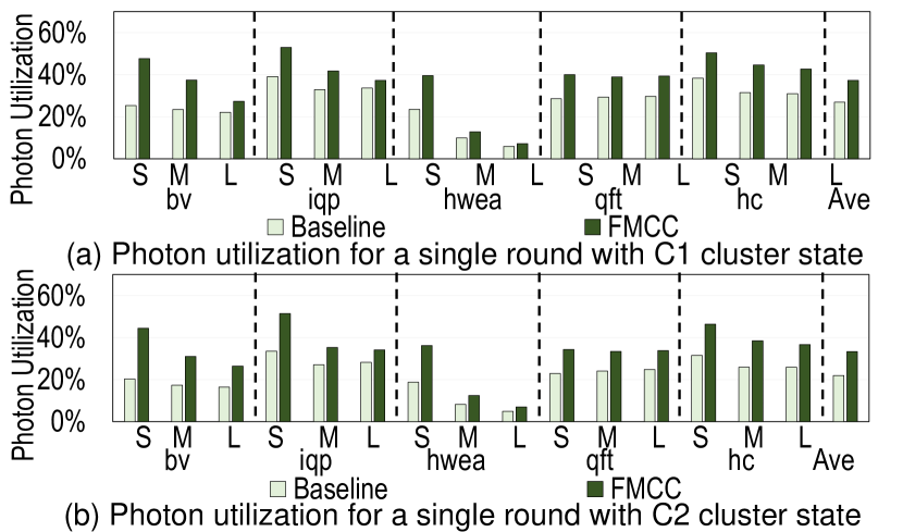
Figure 16. Photon utilization for one round.

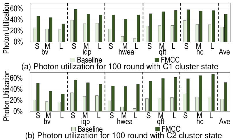
Figure 17. Photon utilization for 100 rounds.

6. Related Works

Super-conducting quantum computation, one of the main paradigms in quantum computation has exhibited great generality and performance in many fields but is still limited by the physical device size and low coherence time. Multiple compilation frameworks  (2qan, ; scm, ; ccmqaoa, ) have been proposed to tackle these challenges and improve fidelity. For example, to address the problem that three-qubit gates are not natively supported at the physical level, gate decomposition (trios, ) and qubits compression (dqw, ) are applied to reduce the overhead introduced when mapping three-qubit gates onto physical devices. Also, to deploy a large-scale quantum circuit onto physical devices with limited size, Qompress (qompress, ) compresses two qubits into one four-state ququart and efficiently routes qubits to reduce communication and extra execution time brought by ququart gates. Besides, CaQR (caqr, ) leverages mid-circuit measurements to reduce qubit usages and the insertion of swap gates, thus leading to higher efficiency in resource utilization. What’s more, because the limited connectivity among physical qubits on super-conducting devices degrades the performance and fidelity of given circuits, SABRE (gushu, ) proposed a SWAP-based algorithm to search for qubit mapping solution to eliminate unnecessary operations, leading to higher efficiency and fidelity of the given circuit. However, the supported quantum gate of the quantum device and the connectivity among physical qubits are no longer concerns in MBQC. Meanwhile, there is a vast difference between the two quantum computation paradigms, thus this previous work cannot be applied to optimize MBQC circuits.

On the other hand, some pioneering steps are taken for leveraging the compilation to improve the fidelity or performance of MBQC. For MBQC based on the graph state, a multi-qubit state represented by a graph with a flexible geometry, it is scaled up by connecting resource states (rs, ) with highly error-prone quantum operations named fusion (fusion, ). To reduce fusions and improve fidelity, several prior works build up the complete compilation flow (gs1, ; gs2, ; oneq, ) and apply the qubit delaying and routing algorithm to eliminate extra fusions. However, these works only focus on fusion reduction while our work targets to reduce the depth of a cluster state that is generated by a variety of techniques (coupleemitter1, ; coupleemitter2, ; pichler2017universal, ; 2023deterministic, ; quantumdot, ), they are not applicable for reducing cluster state depth.

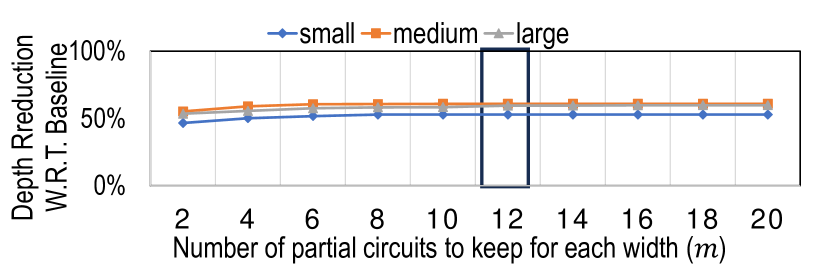
Figure 18. Depth reduction with various of $m$.

7. Conclusion

In this paper, we propose FMCC, which is flexible MBQC computation on cluster state with the goal of minimizing the cluster state depth. The proposed FMCC leverages both intra-component flexibility and inter-component flexibility to effectively utilize the redundant photons and rows in a fixed-width cluster state. Specifically, FMCC employs a dynamic programming approach to reduce the huge design space searching while avoiding sub-optimal results using simple heuristics. Experimental results using five representative quantum applications have shown that, compared to the state-of-the-art MBQC compilation, FMCC achieves 53.6%, 60.6%, and 60.0% average depth reductions in small, medium, and large qubit counts, respectively.

References

- (1) Mahabubul Alam, Abdullah Ash-Saki, and Swaroop Ghosh. Circuit compilation methodologies for quantum approximate optimization algorithm. In 2020 53rd Annual IEEE/ACM International Symposium on Microarchitecture (MICRO), pages 215–228, 2020.
- (2) Frank Arute, Kunal Arya, Ryan Babbush, Dave Bacon, Joseph C Bardin, Rami Barends, Rupak Biswas, Sergio Boixo, Fernando GSL Brandao, David A Buell, et al. Quantum supremacy using a programmable superconducting processor. Nature, 574(7779):505–510, 2019.
- (3) Sara Bartolucci, Patrick Birchall, Hector Bombin, Hugo Cable, Chris Dawson, Mercedes Gimeno-Segovia, Eric Johnston, Konrad Kieling, Naomi Nickerson, Mihir Pant, et al. Fusion-based quantum computation. Nature Communications, 14(1):912, 2023.
- (4) Michael J Bremner, Richard Jozsa, and Dan J Shepherd. Classical simulation of commuting quantum computations implies collapse of the polynomial hierarchy. Proceedings of the Royal Society A: Mathematical, Physical and Engineering Sciences, 467(2126):459–472, 2011.
- (5) Michael J Bremner, Richard Jozsa, and Dan J Shepherd. Classical simulation of commuting quantum computations implies collapse of the polynomial hierarchy. Proceedings of the Royal Society A: Mathematical, Physical and Engineering Sciences, 467(2126):459–472, 2011.
- (6) Hans J Briegel, David E Browne, Wolfgang Dür, Robert Raussendorf, and Maarten Van den Nest. Measurement-based quantum computation. Nature Physics, 5(1):19–26, 2009.
- (7) Yudong Cao, Jonathan Romero, Jonathan P Olson, Matthias Degroote, Peter D Johnson, Mária Kieferová, Ian D Kivlichan, Tim Menke, Borja Peropadre, Nicolas PD Sawaya, et al. Quantum chemistry in the age of quantum computing. Chemical reviews, 119(19):10856–10915, 2019.
- (8) Juan I Cirac and Peter Zoller. Quantum computations with cold trapped ions. Physical review letters, 74(20):4091, 1995.
- (9) Dan Cogan, Zu-En Su, Oded Kenneth, and David Gershoni. Deterministic generation of indistinguishable photons in a cluster state. Nature Photonics, 17(4):324–329, 2023.
- (10) Don Coppersmith. An approximate fourier transform useful in quantum factoring. arXiv preprint quant-ph/0201067, 2002.
- (11) Y. Ding, P. Gokhale, S. Lin, R. Rines, T. Propson, and F. T. Chong. Systematic crosstalk mitigation for superconducting qubits via frequency-aware compilation. In 2020 53rd Annual IEEE/ACM International Symposium on Microarchitecture (MICRO), pages 201–214, Los Alamitos, CA, USA, oct 2020. IEEE Computer Society.
- (12) Casey Duckering, Jonathan M. Baker, Andrew Litteken, and Frederic T. Chong. Orchestrated trios: Compiling for efficient communication in quantum programs with 3-qubit gates. In Proceedings of the 26th ACM International Conference on Architectural Support for Programming Languages and Operating Systems, ASPLOS ’21, page 375–385, New York, NY, USA, 2021. Association for Computing Machinery.
- (13) Sophia E Economou, Netanel Lindner, and Terry Rudolph. Optically generated 2-dimensional photonic cluster state from coupled quantum dots. Physical review letters, 105(9):093601, 2010.
- (14) Mercedes Gimeno-Segovia, Terry Rudolph, and Sophia E Economou. Deterministic generation of large-scale entangled photonic cluster state from interacting solid state emitters. Physical review letters, 123(7):070501, 2019.
- (15) Mercedes Gimeno-Segovia, Pete Shadbolt, Dan E. Browne, and Terry Rudolph. From three-photon greenberger-horne-zeilinger states to ballistic universal quantum computation. Phys. Rev. Lett., 115:020502, Jul 2015.
- (16) Lov K Grover. A fast quantum mechanical algorithm for database search. In Proceedings of the twenty-eighth annual ACM symposium on Theory of computing, pages 212–219, 1996.
- (17) Robert H Hadfield. Single-photon detectors for optical quantum information applications. Nature photonics, 3(12):696–705, 2009.
- (18) Fei Hua, Yuwei Jin, Yanhao Chen, Suhas Vittal, Kevin Krsulich, Lev S. Bishop, John Lapeyre, Ali Javadi-Abhari, and Eddy Z. Zhang. Caqr: A compiler-assisted approach for qubit reuse through dynamic circuit. In Proceedings of the 28th ACM International Conference on Architectural Support for Programming Languages and Operating Systems, Volume 3, ASPLOS 2023, page 59–71, New York, NY, USA, 2023. Association for Computing Machinery.
- (19) Richard Jozsa. An introduction to measurement based quantum computation. NATO Science Series, III: Computer and Systems Sciences. Quantum Information Processing-From Theory to Experiment, 199:137–158, 2006.
- (20) Lingling Lao and Dan E. Browne. 2qan: A quantum compiler for 2-local qubit hamiltonian simulation algorithms. In Proceedings of the 49th Annual International Symposium on Computer Architecture, ISCA ’22, page 351–365, New York, NY, USA, 2022. Association for Computing Machinery.
- (21) Mikkel V Larsen, Xueshi Guo, Casper R Breum, Jonas S Neergaard-Nielsen, and Ulrik L Andersen. Deterministic generation of a two-dimensional cluster state. Science, 366(6463):369–372, 2019.
- (22) Gushu Li, Yufei Ding, and Yuan Xie. Tackling the qubit mapping problem for nisq-era quantum devices. In Proceedings of the Twenty-Fourth International Conference on Architectural Support for Programming Languages and Operating Systems, pages 1001–1014, 2019.
- (23) Yingheng Li, Aditya Pawar, Mohadeseh Azari, Guo Yanan, Youtao Zhang, Jun Yang, Kaushik Seshadreesan, and Xulong Tang. Orchestrating measurement-based quantum computation over photonic quantum processors. In Proceedings of the 60th ACM/IEEE Design Automation Conference, 2023.
- (24) Andrew Litteken, Lennart Maximilian Seifert, Jason Chadwick, Natalia Nottingham, Frederic T. Chong, and Jonathan M. Baker. Qompress: Efficient compilation for ququarts exploiting partial and mixed radix operations for communication reduction. In Proceedings of the 28th ACM International Conference on Architectural Support for Programming Languages and Operating Systems, Volume 2, ASPLOS 2023, page 646–659, New York, NY, USA, 2023. Association for Computing Machinery.
- (25) Andrew Litteken, Lennart Maximilian Seifert, Jason D. Chadwick, Natalia Nottingham, Tanay Roy, Ziqian Li, David Schuster, Frederic T. Chong, and Jonathan M. Baker. Dancing the quantum waltz: Compiling three-qubit gates on four level architectures. In Proceedings of the 50th Annual International Symposium on Computer Architecture, ISCA ’23, New York, NY, USA, 2023. Association for Computing Machinery.
- (26) Ji Liu, Peiyi Li, and Huiyang Zhou. Not all swaps have the same cost: A case for optimization-aware qubit routing. In 2022 IEEE International Symposium on High-Performance Computer Architecture (HPCA), pages 709–725. IEEE, 2022.
- (27) Nikolaj Moll, Panagiotis Barkoutsos, Lev S Bishop, Jerry M Chow, Andrew Cross, Daniel J Egger, Stefan Filipp, Andreas Fuhrer, Jay M Gambetta, Marc Ganzhorn, et al. Quantum optimization using variational algorithms on near-term quantum devices. Quantum Science and Technology, 3(3):030503, 2018.
- (28) Michael A Nielsen and Isaac L Chuang. Quantum computation and quantum information. Phys. Today, 54(2):60, 2001.
- (29) Jeremy L O’brien. Optical quantum computing. Science, 318(5856):1567–1570, 2007.
- (30) Jeremy L O’brien, Akira Furusawa, and Jelena Vučković. Photonic quantum technologies. Nature Photonics, 3(12):687–695, 2009.
- (31) Hannes Pichler, Soonwon Choi, Peter Zoller, and Mikhail D Lukin. Universal photonic quantum computation via time-delayed feedback. Proceedings of the National Academy of Sciences, 114(43):11362–11367, 2017.
- (32) Robert Raussendorf and Hans J Briegel. A one-way quantum computer. Physical review letters, 86(22):5188, 2001.
- (33) Robert Raussendorf, Daniel E Browne, and Hans J Briegel. Measurement-based quantum computation on cluster states. Physical review A, 68(2):022312, 2003.
- (34) Robert Raussendorf and Tzu-Chieh Wei. Quantum computation by local measurement. Annu. Rev. Condens. Matter Phys., 3(1):239–261, 2012.
- (35) Adam Sawicki, Lorenzo Mattioli, and Zoltán Zimborás. Universality verification for a set of quantum gates. Physical Review A, 105(5):052602, 2022.
- (36) Peter W Shor. Polynomial-time algorithms for prime factorization and discrete logarithms on a quantum computer. SIAM review, 41(2):303–332, 1999.
- (37) Sergei Slussarenko and Geoff J Pryde. Photonic quantum information processing: A concise review. Applied Physics Reviews, 6(4):041303, 2019.
- (38) Nicholas H Stair, Renke Huang, and Francesco A Evangelista. A multireference quantum krylov algorithm for strongly correlated electrons. Journal of chemical theory and computation, 16(4):2236–2245, 2020.
- (39) Ravitej Uppu, Leonardo Midolo, Xiaoyan Zhou, Jacques Carolan, and Peter Lodahl. Quantum-dot-based deterministic photon–emitter interfaces for scalable photonic quantum technology. Nature nanotechnology, 16(12):1308–1317, 2021.
- (40) Arian Vezvaee, Paul Hilaire, Matthew F Doty, and Sophia E Economou. Deterministic generation of entangled photonic cluster states from quantum dot molecules. Physical Review Applied, 18(6):L061003, 2022.
- (41) Madhav Krishnan Vijayan, Alexandru Paler, Jason Gavriel, Casey R. Myers, Peter P. Rohde, and Simon J. Devitt. Compilation of algorithm-specific graph states for quantum circuits. 2022.
- (42) Hezi Zhang, Anbang Wu, Yuke Wang, Gushu Li, Hassan Shapourian, Alireza Shabani, and Yufei Ding. Oneq: A compilation framework for photonic one-way quantum computation. In Proceedings of the 50th Annual International Symposium on Computer Architecture, pages 1–14, 2023.
- (43) Felix Zilk, Korbinian Staudacher, Tobias Guggemos, Karl Fürlinger, Dieter Kranzlmüller, and Philip Walther. A compiler for universal photonic quantum computers. 2022.