Abstract

Material characterization in nano-mechanical tests requires precise interatomic potentials for the computation of atomic energies and forces with near-quantum accuracy. For such purposes, we develop a robust neural-network interatomic potential (NNIP), and we provide a test for the example of molecular dynamics (MD) nanoindentation, and the case of body-centered cubic crystalline molybdenum (Mo). We employ a similarity measurement protocol, using standard local environment descriptors, to select ab initio configurations for the training dataset that capture the behavior of the indented sample. We find that it is critical to include generalized stacking fault (GSF) configurations, featuring a dumbbell interstitial on the surface, to capture dislocation cores, and also high-temperature configurations with frozen atom layers for the indenter tip contact. We develop a NNIP with distinct dislocation nucleation mechanisms, realistic generalized stacking fault energy (GSFE) curves, and an informative energy landscape for the atoms on the sample surface during nanoindentation. We compare our NNIP results with nanoindentation simulations, performed with three existing potentials—an embedded atom method (EAM) potential, a gaussian approximation potential (GAP), and a tabulated GAP (tabGAP) potential—that predict different dislocation nucleation mechanisms, and display the absence of essential information on the shear stress at the sample surface in the elastic region. We believe that these features render specialized NNIPs essential for simulations of nanoindentation and nano-mechanics with near-quantum accuracy.

I Introduction

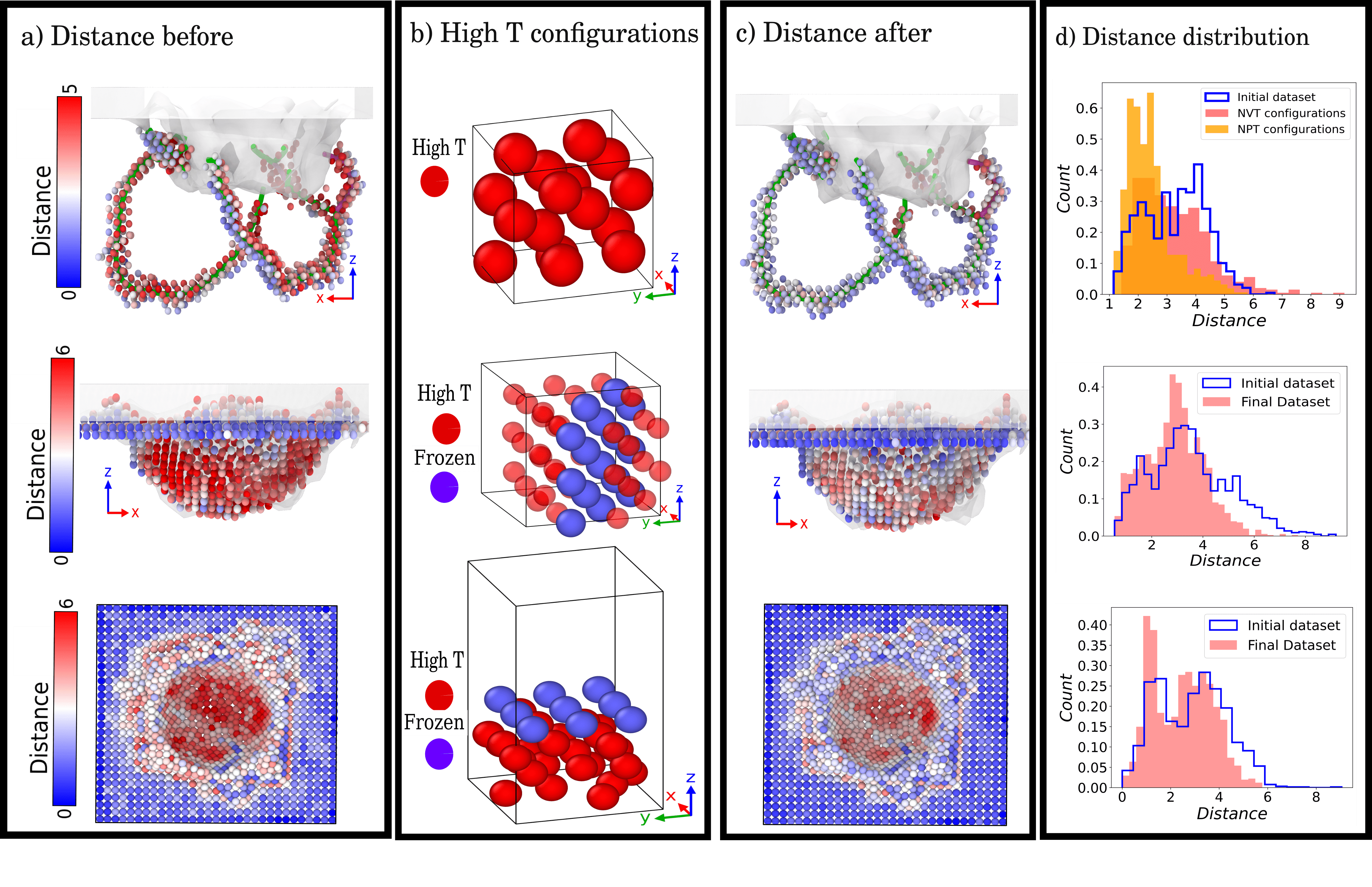
Figure 1: Illustration of the novel configurations discovered in this study, which correspond to distinct regions of an indented sample. The figures are arranged horizontally to demonstrate the correlation between them. a) The distances of the dislocation cores, atoms beneath the indenter tip, and pileup atoms on the surface from the original dataset. b) The newly detected high-temperature configurations, which are associated with diverse regions of the indented sample, in terms of their distance. c) The distance of the aforementioned regions shown in panel (a) after incorporating the newly found configurations to the dataset. d) The distribution of distances of the aforementioned atoms from the dataset before and after incorporating the newly introduced configurations.

Nano-mechanical tests serve as essential tools for probing the mechanical properties of materials at the nanoscale. Techniques such as nano-tensile/compression Kim and Greer (2009); Kim et al. (2012); Motamedi et al. (2020), nanoindentation  Schuh (2006); Varillas et al. (2017); Kurpaska et al. (2022); Pathak and Kalidindi (2015); Voyiadjis and Yaghoobi (2017); Remington et al. (2014); Gagel et al. (2016); Naghdi et al. (2022), and creep testing  Taneike et al. (2003) play a pivotal role in revealing the intrinsic properties of materials. This understanding, in turn, facilitates the design and production of innovative materials capable of functioning in extreme environments. These tests involve subjecting the material to controlled strain/stress at the nanoscale, enabling researchers to gain valuable insights into its mechanical response. This knowledge is crucial in the field of defect physics, as nano-mechanical tests provide a means to investigate the mechanisms of defects nucleation and their impact on the mechanical performance of materials under extreme conditions. In this study, we aim to present a comprehensive method for simulating nano-mechanical tests, taking nanoindentation as an example, on crystalline materials using neural-network interatomic potentials (NNIPs).

Nano-mechanical test techniques find application in a several areas of materials science. Specifically, in situ techniques  Haque and Saif (2002); De Hosson et al. (2006) contribute significantly to the understanding of material deformation under controlled applied stress or strain, while the specimen is simultaneously observed/measured by electron microscopic devices. These methodologies play a pivotal role in exploring materials properties at the nano scale, offering insights into the intrinsic properties of materials, such as the strength of each crystalline grain. Furthermore, these techniques prove invaluable in investigating temperature- related deformation mechanisms inherent in crystalline materials. The focus of this paper is on nanoindentation testing, a widely utilized method for assessing material properties on open surfaces. This technique yields results for various properties, encompassing hardness, strength, dislocation nucleation mechanisms, dislocation density, grain boundary effects, and dislocation junction formations  Durst et al. (2005); Maier-Kiener et al. (2017); Casals et al. (2007); Smith et al. (2003); Swaddiwudhipong et al. (2006); Dominguez-Gutierrez et al. (2021); Kramer et al. (2001); Biener et al. (2007); Voyiadjis and Faghihi (2012); Plummer (2019). However, it is essential to note that nanoindentation testing involves intricate defect nucleation mechanisms and plastic deformations, rendering accurate modeling a formidable challenge within the realm of computational materials science.

Various computational methods, such as finite element methods (FEM)  Frydrych et al. (2023); Knapp et al. (1999); Lichinchi et al. (1998), discrete dislocation dynamics (DDD)  Zhou et al. (2010); Motz et al. (2008); Song et al. (2019), and molecular dynamics (MD)  Xu et al. (2024); Domínguez-Gutiérrez et al. (2023); Naghdi et al. (2023); Karimi et al. (2023); Karimi and Papanikolaou (2023), are employed for modeling nano-mechanical testing. In FEM, numerical solutions to differential equations in mathematical models are used to approximate and analyze the complex behavior of materials. While FEM is useful in certain cases, it lacks atomic-level information and, therefore, does not achieve quantum accuracy. DDD simulations explicitly describe dislocation dynamics at the mesoscale, but are limited in predicting defect properties with quantum-level accuracy. In contrast, MD simulations can provide atomic-level insights into the dislocation dynamics of materials, given the use of interatomic potentials finely tuned for nano-mechanics in the simulations.

Machine-learned force fields (MLFFs)  Behler and Parrinello (2007); Bartók et al. (2010); Thompson et al. (2015); Shapeev (2016); Glielmo et al. (2018); Zhang et al. (2018); Behler (2016); Shaidu et al. (2021); Li et al. (2021) offer a reliable means for modeling nano-mechanical tests with quantum-level accuracy. Various MLFF types, such as Gaussian Approximation Potentials (GAP)  Bartók et al. (2010) and its tabulated version (tabGAP)  Byggmästar et al. (2022), as well as active learning methods like FLARE  Vandermause et al. (2020), are available in the literature. In addition, NNIPs exhibit exceptional accuracy in predicting atomic energies and forces  Pellegrini et al. (2023); Musaelian et al. (2023); Batatia et al. (2022), overcoming the time and system size limitations inherent in traditional ab initio molecular dynamics (AIMD) simulations. Given the ability of NNIPs to learn complex functions, such as the energy landscape of an extended dislocation in a metallic crystal, they prove to be excellent tools for modeling nano-mechanical testing simulations. MLFFs have been successfully applied to various problems, including catalysis  Owen et al. (2023a, b), point defects modeling  Goryaeva et al. (2021); Byggmästar et al. (2019), multi- component materials modeling Nikoulis et al. (2021); Byggmästar et al. (2021), and multi-phase systems  Shaidu et al. (2021), demonstrating their versatility. However, the exploration of nano-mechanical testing simulations using MLFFs is an area that remains to be fully explored.

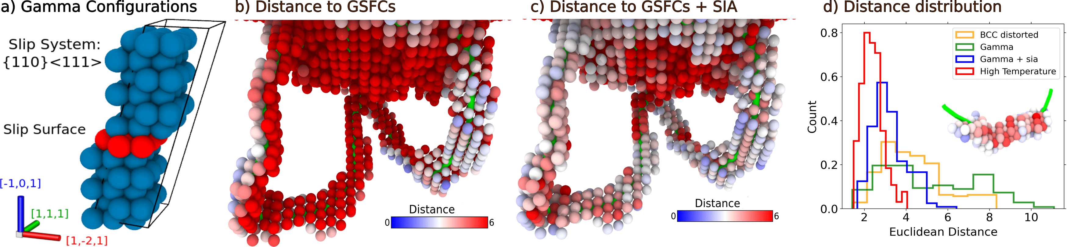
Figure 2: The impact of incorporating GSFCs on the distances of atoms on dislocation cores from the dataset. a) A schematic representation of the GSFCs integrated into the dataset. b) Addition of GSFCs reduces the distances of atoms on the slip plane of dislocation cores from the dataset. c) By including a SIA on the surface of GSFCs, all atoms on the dislocation cores can be covered. d) The distribution of atom distances on dislocation cores reveals that GSFCs with SIA can effectively cover dislocation cores.

In this paper, we present a study focused on the development of a quantum-level-accurate NNIP by enhancing a starting dataset sourced from the literature  Byggmästar et al. (2020a) within the PANNA (Properties from Artificial Neural Network Architectures) framework  Lot et al. (2020). We compare the Behler-Parrinello descriptor vectors  Behler and Parrinello (2007) of the training dataset with those of a single crystal BCC Molybdenum configuration, indented with an embedded atom model (EAM) potential  Salonen et al. (2003), to determine how closely the training dataset resembles the indentation process. To improve the accuracy of the potential, we introduce high temperature configurations with a frozen layer and generalized stacking fault (GSF) configurations with an interstitial on the gamma surface. These configurations are designed to closely mimic atoms in the dislocation cores, on the surface, and under the indenter tip. Our results show that including these configurations in the training dataset reduces the distance between the atoms the potential is trained on and the indented sample. Finally, we present the results of an MD nanoindentation simulation using the potential trained with the modified dataset.

II Results

II.1 NNIP Dataset Explores the Intricacies of Every Atomic Landscape During Nanoindentation

First, we applied a similarity measurement methodology, resulting in an ideal dataset for nano-mechanical applications, particularly in the context of nanoindentation simulations. This method assesses similarity by comparing distances between atoms in two configurations/datasets, using modified Behler-Parinnelo descriptors  Smith et al. (2017); Behler and Parrinello (2007). Then it focuses on finding the ”largest minimum” distance of atomic descriptors in two configurations/datasets (see Methods). We employed this method for comparing configuration types in a dataset from literature Byggmästar et al. (2020a) to atomic landscapes in an indented sample accuaired with empirical methods  Salonen et al. (2003), aiming to gain insights into the dataset’s suitability for studying nanoindentation behavior and uncovering underlying mechanisms.

To curate a well-designed dataset for the nanoindentation of single crystalline Molybdenum (Mo), we identified unique configurations with a close distance to defected regions of an indented configuration. This encompasses point defects, situated near the sample surface, as well as extended defects like dislocation lines and junctions. Fig.1(a) summarizes the three defected regions, and their color-coded distance to the initial dataset, of an indented sample. This includes the extended dislocation lines and junctions (top), point defects under the indenter tip (middle) and the surface atoms (bottom). An interatomic potential employed for nano-mechanical simulations must effectively capture the intricate energy landscape of defects that arise during the simulation. Consequently, we identified distinctive configurations to ensure comprehensive coverage of this complexity (Fig. 1(b)). Our findings suggest that high-temperature NPT configurations, in contrast to NVT configurations, have a close distance to dislocation cores. Additionally, it was observed that these configurations address the defected regions beneath the indenter tip when a layer of atoms is kept frozen. The ultimate refinement of the dataset is optimized by introducing a void atop high-temperature configurations with the frozen layers, particularly benefiting the surface atoms. The effect of aformentioned dataset modifications is demonstrated in Fig.1(c-d). Ultimately, the distances between atoms from the indented sample and the dataset are reduced, evident in the narrowing of the distance distribution width.

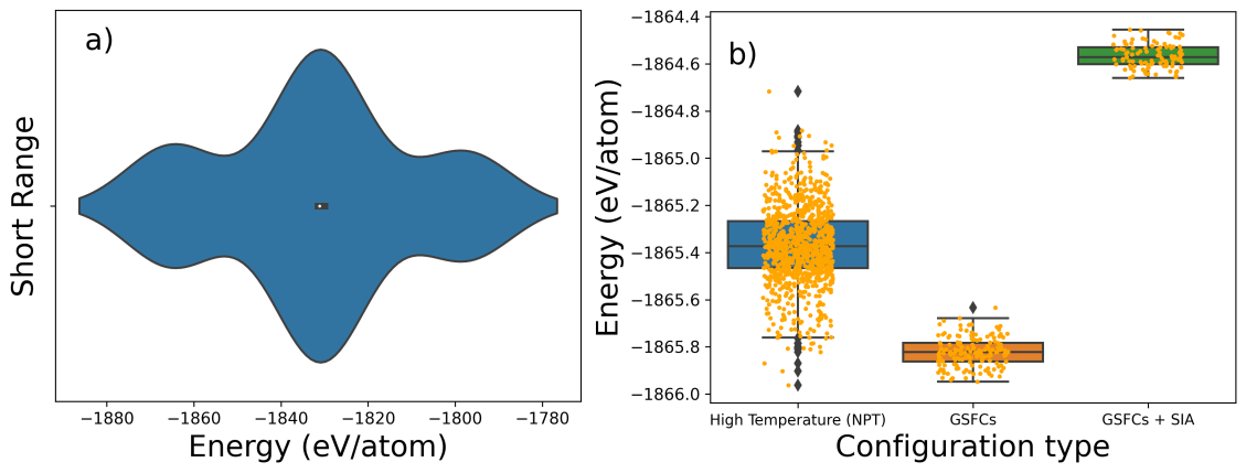
Figure S1: Energy distribution of a) Short range configurations and b) High temperature and GSFCs. The drastic variation of energies for short range configurations (100 meV/atom) suggest that these configurations would be problematic for training a NNIP. n addition, it is shown that although high temperature NPT configurations have a larger energy distribution than the GSFCs.

Moreover, it was also observed that Generalized Stacking Fault Configurations (GSFCs) incorporating a dumbbell self-interstitial atom (SIA) on the top have a close distance to atoms within the dislocation cores. A representative GSFC is illustrated in Fig.2(a). A GSFC without any point defects would solely exhibit proximity to the atoms on the plane where the dislocation is slipping, which is shown in Fig.2(b). GSFCs with a dumbbell interstitial positioned near the $\gamma$-surface (the slip surface), on the other hand, were found to be in close proximity to the dislocation cores (Fig.2(c)). This outcome is further evident in the distance distributions depicted in Fig. 2(d). Distorted BCC and GSF configurations exhibit a tail surpassing the distance threshold, whereas high NPT high-temperature configurations along with GSFCs + SIA display a smaller tail. However, the high-temperature configurations were excluded from the training set due to their substantial energy variation, introducing challenges in effectively training a NNIP (Fig.S1(b)). GSFCs, on the other hand happen to have a smaller energy variation, which suggests a more accurate prediction for dislocation cores and also is closer to the concept of a defect in crystalls. GSFCs, conversely, exhibit a significantly smaller energy variation. This implies a more precise prediction for dislocation cores and aligns more closely with the concept of defects in crystals. Ultimately, the dataset for the NNIP is meticulously crafted, making it ideal for nanoindentation simulations. For a more detailed description of the distance metric and the configurations considered, please see Methods.

II.2 NNIP Validations

II.2.1 NNIP Achieves Quantum-Accurate Predictions for Energies and Forces

We assessed the accuracy of the trained NNIP by calculating the root mean square error (RMSE) for both energies per atom (E-RMSE) and forces components (F-RMSE) at each checkpoint saved during training. To ensure the reliability of the final model on unseen data, $10\%$ of configurations of each structure type were reserved for validation prior to training. Fig. 3 shows that both the F-RMSE and E-RMSE decrease gradually as the network processes more data, reaching a plateau after 850K training steps with minimum values of 9.2 meV/atom and 0.16 eV/Å, respectively.

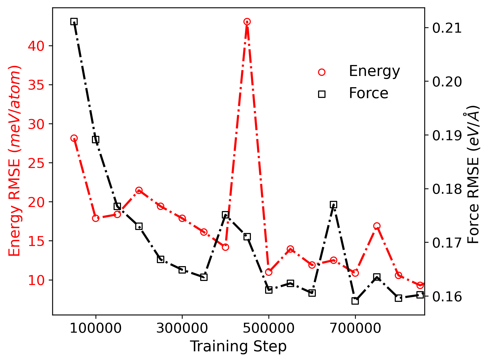
Figure 3: Prediction of the Energies and forces for the validation set during the NNIP training.

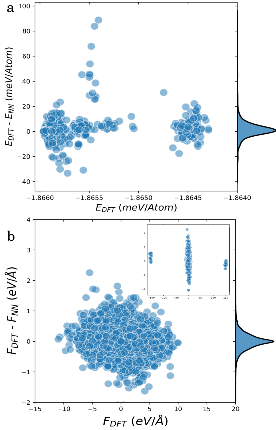
Figure 4: NNIP error on (a) total energies and (b) forces of each atom.

The error distribution for both energies and forces are shown in the histogram plot of Fig. 4(a,b). The two islands in Fig. 4(a) are due to the energy difference between the pure and defected crystals. Also, the presence of three clusters in Fig. 4(b) is due to the large forces on the atoms in the defected configurations.

	GAP	tabGap	EAM	NNIP	DFTa	DFTb	Expc
$C_{11}$ (GPa)	478 (3.02%)	494 (6.47%)	465 (0.22%)	452 (2.59%)	459	468	464
$C_{12}$ (GPa)	166 (4.40%)	146 (8.18%)	161 (1.26%)	121 (23.90%)	162	155	159
$C_{44}$ (GPa)	108 (0.92%)	87 (20.18%)	109 (0%)	111 (1.83%)	97	100	109
$B$ (GPa)	270 (8.00%)	262 (4.80%)	263 (5.20%)	231 (7.60%)	262	-	250
$\nu$	0.26 (10.34%)	0.23 (20.69%)	0.26 (10.34%)	0.21 (27.59%)	0.30	-	0.29
a This work.
b Reference Byggmästar et al. (2020a)   .
c Reference Rumble (2019).

Table 1: Elastic constants $C_{ij}$, bulk modulus $B$, and Poisson ratio $\nu$, as obtained with the GAP, tabGAP, EAM/FS and the NNIP potentials compared to DFT done in this work and experimental data. In parenthesis is reported the modulus of the percentage error with respect to the experimental value.

II.2.2 Bulk Validation

Next, we compare the elastic properties of the NNIP interatomic potential with both DFT and experimental results, as well as to those predicted by other interatomic potentials, such as GAP, tabGAP, and the EAM/FS potential, to evaluate the NNIP performance relative to other commonly used potentials. Table. 1 summarizes the results of the comparison, explicitly reporting percentage errors with respect to the experimental values. The NNIP performs well for $C_{11}$, $C_{44}$ and $B$, with percentage errors below $8\%$ and in similar magnitude to GAP and EAM predictions. We here stress that the accurate prediction of the shear modulus, $C_{44}$, is crucial for simulating the stresses that are applied to the surface of the sample during nanoindentation, and, following the good results of EAM and GAP for this measure, the NNIP proves itself to be promising for such applications. While the largest error for the NNIP concerns the prediction of $C_{12}$, it can still be considered within a reasonable range as it does not exceedingly influence the prediction on $B$.

II.2.3 NNIP Accurately Predicts Generalized Stacking Fault Energies (GSFE)

Finally, we compare the NNIP predictions for the GSFE against the DFT results, as well as other interatomic potentials mentioned in this work. The study focuses on the two most important slip systems of BCC crystals, namely the $\{110\}\langle\bar{1}11\rangle$ and $\{121\}\langle\bar{1}11\rangle$ families. The results were obtained for these directions in pure crystals. Additionally, since it was observed from Fig. 2 that GSF $\{110\}\langle 111\rangle$ configurations with a $\langle 111\rangle$ dumbbell interstitial on the surface are essential to cover the atomic environments of the dislocation core in terms of their distance to the indented samples, we also calculated and compared the GSFE for these configurations.

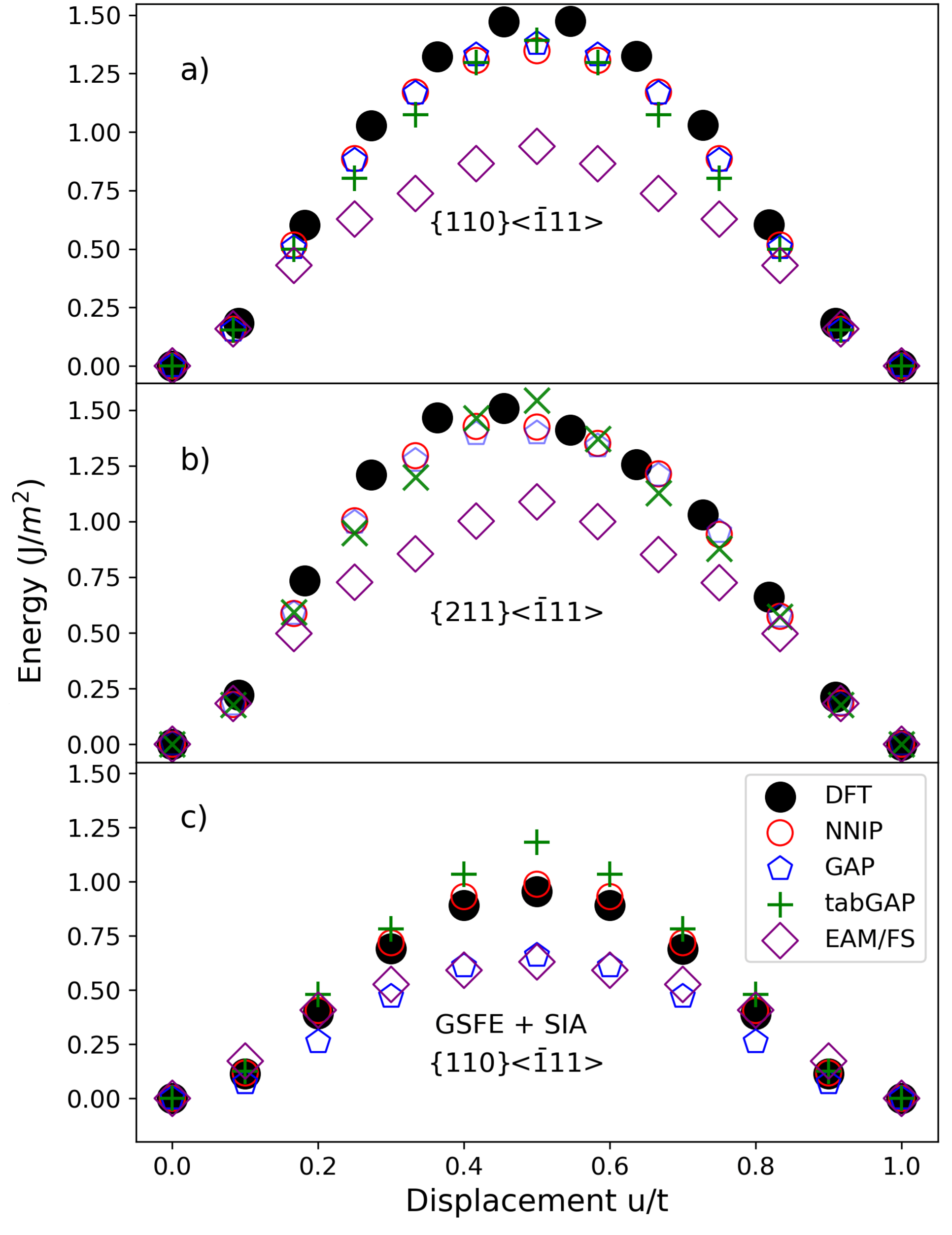
Figure 5: Generalized Stacking Fault Energy (GSFE) for single crystalline Molybdenum for: (a) $\{110\}\langle\bar{1}11\rangle$ and (b) $\{211\}\langle\bar{1}11\rangle$. (c) The GSFE curve for the ”GSFCs $+$ SIA” configurations.

Fig. 5 shows that all potentials predict the GSFE very accurately for both slip system families and pure crystals. However, EAM/FS displays errors of about $50\%$ and $32\%$ for the peak of the curve for $\{110\}\langle\bar{1}11\rangle$ and $\{121\}\langle\bar{1}11\rangle$ slip families, respectively. The configurations associated with these curves are crucial, as they represent the atoms on the slip plane of an indented sample, as illustrated and discussed in Fig. 2. While it is important for an interatomic potential to accurately predict the GSFE curve for reliable dislocation modeling, it is equally crucial for the potential to correctly predict the energies and forces on the atoms for the dislocation cores. Therefore, in addition to the GSFE curves for pure crystals, we calculated the GSFE curve for configurations with a $\langle 111\rangle$ dumbbell interstitial on the surface. As depicted in Fig. 5(c), NNIP is the potential that best predicts these energies, indicating the accurate simulation of dislocation dynamics during nanoindentation. In contrast, GAP and EAM potentials showed errors of $40\%$ and tabGAP showed an error of $20\%$ against DFT results, indicating their inability to accurately predict these values. This is discussed further in the following section.

II.3 NNIP Nanoindentation predictions

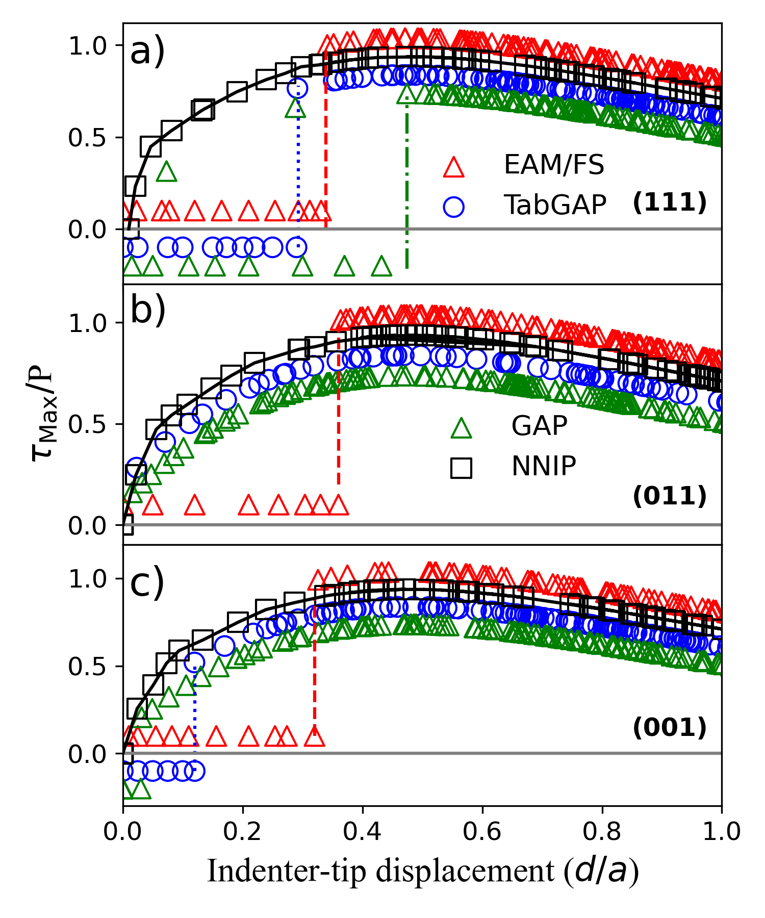
Figure 6: Hertzian calculation of normalized maximum shear stress by the applied pressure, $\tau_{\rm max}/P$, as a function of normalized depth for main crystal orientations. Surface information is needed in the interatomic potentials to model nanoindentation induced plasticity in the range of 0.0 to 0.475 $d/a$. To aid the interpretation of the results, the values for EAM/FS were shifted by $-0.1$, the values for GAP were shifted by $+0.2$, and the values for tabGAP were shifted by $+0.1$ (all values in units of $\tau_{\rm max}/P$).

Plastic deformation does not initiate at the surface, but rather at a certain depth below it, typically a few atomic layers deep. This depth is known as the “yield point” or “yield depth”, at which point the material begins to nucleate defects and dislocations under the applied load or stress. The initiation of the plastic deformation of the material occurs within the closest plastic region along the vertical $z$-axis beneath the spherical indenter tip. In Fig. 6 we show results for the normalized maximum shear stress $\tau_{\rm max}/P$ which is a dimensionless quantity, with $P$ being the applied pressure (Eq. 13) and $\tau_{\rm max}$ the shear stress (Eq. 17) calculated by using a linear elastic contact mechanics formulation Domínguez-Gutiérrez et al. (2023); Varillas et al. (2017), as a function of the displacement $d$ for [001], [011], and [111] main crystal orientations Domínguez-Gutiérrez et al. (2023). A detailed explanation of the normalized shear stress calculation is provided in the Methods section.

Our MD simulations report enough surface energy to model the nanoindentation induced plasticity as observed at distances close to the sample surface regardless of the crystal orientation, which is challenging for traditional and current ML interatomic potentials for BCC Mo. The modeling of the nanocontact of the indenter tip and the top atomic layers of the surface, from 0 to $\sim 0.3$ $d/a$ range with $d$ the indentation depth and $a$ the contact area, is important due to the nucleation of dislocation being dependent on this mechanisms.

The GAP simulations provide valuable insights into the interaction between the indenter tip and the top layer atoms for the (001) and (011) orientations. However, for the (111) orientation, this information is lacking, resulting in a limitation in accurately modeling the nanoindentation test before the yield point. This limitation arises due to the absence of the relevant atomic configurations in the training data for this specific potential. As a consequence, the tabGAP simulations follow a similar trend for the (111) orientation, reflecting the lack of detailed information on the interaction between the tip and the surface atoms.

In contrast, the NNIP simulations incorporate sufficient information on surface structures, allowing for a more accurate representation of the contact area. This is particularly important as the contact area depends on the applied load. The computed force between the tip and the atoms comprising the contact area is well-modeled in the NNIP simulations. The difference in spacing between data points in the elastic part of the graph is attributed to variations in the loading force, pressure, and maximum shear stress, which are considered in the contact area analysis.

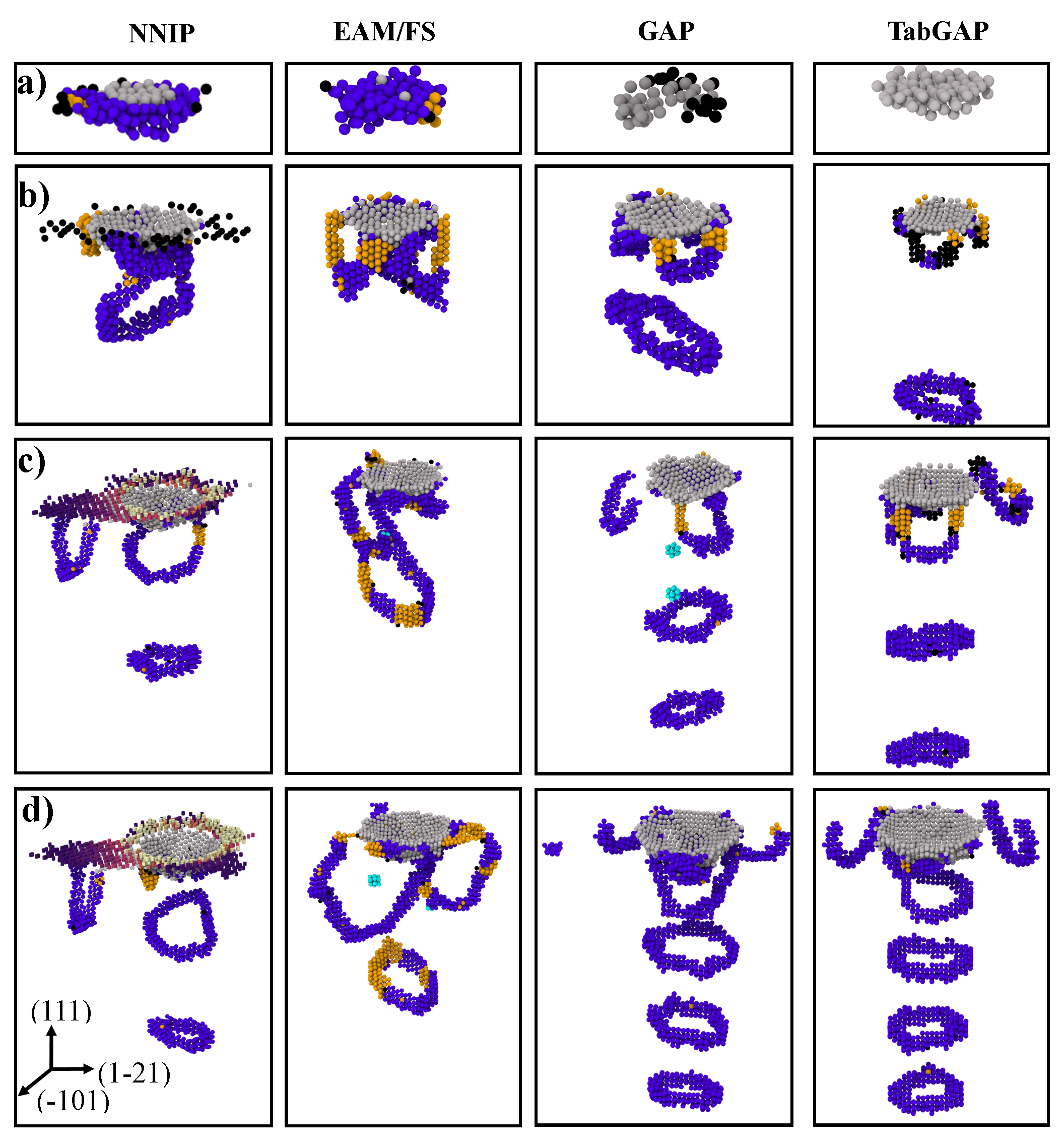
Figure 7: Identified defects of indented (111) Mo sample by BDA method at different depths by NNIP, EAM, TabGAP, and GAP approaches. The various defect types are depicted using different colors: gray spheres represent surface atoms in direct contact with the indenter tip, blue spheres indicate edge dislocations, light-blue spheres represent atoms in the vicinity of vacancies, yellow spheres depict twin/screw dislocations, and black spheres highlight unidentified defect atoms. The nucleation and propagation of edge dislocations on the {111} slip family are observed, which then evolve into prismatic loops. In addition, identified slip traces and pile-ups are well modeled by NNIP simulations showing the well–known three-fold symmetric rosette depths below 1.45 nm that are formed by [11$\bar{2}$], [$\bar{1}$01] and [0$\bar{1}$1] planes.

Fig. 7 illustrates the defects detected using the BCC Defect Analysis (BDA) method (see Methods) in a (111) Mo sample at different depths Möller and Bitzek (2016). The NNIP nanoindentation simulations in the initial stages of loading process notably enhance the description of the interaction between the indenter tip and the atoms in the uppermost layers of the surface (see Fig. 7(a)). In this context, a few Mo atoms located at the very top surface layer are recognized as surface defects. Additionally, Mo atoms situated beneath these surface defects begin to coalesce, forming edge dislocations that have the potential to evolve into shear loops, contrary to the other simulations where the interatomic potentials are not aware of this mechanism. NNIP simulations are also anticipated to accurately capture the nucleation and propagation of shear loops on {112} planes (See Fig. 7(b)), as observed experimentally in BCC materials Varillas et al. (2017); Remington et al. (2014); Mulewska et al. (2023). Furthermore, NNIP effectively models the nucleation of loops through a lasso mechanism, a behavior where GAP and tabGAP induced the formation of multiple loops, as observed in Fig. 7(c)) at a depth of 1.45nm. For NNIP, at the maximum indentation depth, it is evident on the sample’s surface that displaced atoms align with the slip planes in a characteristic three–folded rosette pattern typical for BCC materials in the [111] orientation (Fig. 7(d)), formed by [11$\bar{2}$], [$\bar{1}$01], and [0$\bar{1}$1] planes. In contrast, neither GAP nor tabGAP, nor EAM, can adequately incorporate this description due to the lack of information regarding pile–up formations. Besides, the nucleation of more loops is noted, but the circumference of the second loop is larger than that of the first loop. The EAM and tabGAP simulations demonstrate a slower and faster process, respectively.

In Fig. 8, we display the atomic displacement mapping of the [111] Mo sample obtained by NNIP in (a), EAM/FS in (b), GAP in (c), and tabGAP in (d) at the maximum indentation depth. The surface of the sample clearly shows displaced atoms aligned with the slip planes, forming the characteristic three-fold rosette pattern typical for BCC materials in the [111] orientation, as illustrated by the NNIP results in Fig. 8(a)). This pattern is created by [11$\bar{2}$], [$\bar{1}$01], and [0$\bar{1}$1] planes Kurpaska et al. (2022); Varillas et al. (2017). To assist in identifying the shape of the rosette, we have added orange lines, reminiscent of what can be observed in SEM images of BCC materials Remington et al. (2014). Here NNIP simulations are in good agreement with typical observations of pile–up evolution. However, it is important to note that neither GAP, tabGAP, nor EAM can provide a comprehensive description due to their lack of information about open boundary simulation under external loading.

III Discussion and conclusions

Interatomic potentials developed before the present work, although adequate for many applications, need to be improved for nanoindentation simulations. For example, J. Byggmästar et. al. Byggmästar et al. (2020a) developed a GAP potential for Mo, demonstrating accuracy and transferability for elastic, thermal, liquid, defect, and surface properties. However, this potential failed to produce reliable data for the shear stress in the elastic region in the early stages of the nanoindentation simulation. Furthermore, in contrast to the NNIP developed here, many prismatic loops were nucleated during the nanoindentation (see Fig. 7), potentially due to insufficient information in the energy landscape regarding the dislocation cores, a fact that was illustrated based on the similarity of the GSF configurations with the dislocation cores as depicted in Fig. 5.

The tabGAP potentials are designed for complex multi-element materials Byggmästar et al. (2022), employing simple low-dimensional descriptors. Although tabGAP potentials have notable accuracy for entropy alloys Byggmästar et al. (2021), the same issues as the GAP potential arise when it comes to single element BCC Mo. As mentioned earlier, the tabGAP potential leads to nucleation of too many prismatic dislocation loops in the nanoindentation simulations (see Fig. 7). Moreover, accurate predictions of shear stress in the initial phases of the nanoindentation simulations were not achieved.

The EAM/FS potential utilized in the present work  Salonen et al. (2003), originally designed for radiation damage simulations, failed to accurately produce GSFE curve for Mo in both pristine crystalline and GSF configurations representing dislocation cores. Consequently, it is unclear whether or not this potential can reliably predict dislocation nucleation during indentation. In addition, similar to the other potentials, it does not correctly predict the nanoindentation shear stress.

Considering the challenges faced in nanoindentation simulations, the presence of a well-developed methodology to tackle these issues would be highly beneficial. In this work, we met this goal by introducing to the training dataset new configurations which resemble the local atomic environments of an indented sample. The similarity measurements presented here ensure the relevance of the newly introduced structures to a nanoindentation simulation. To the best of our knowledge, this study represents the first attempt to develop a MLFF specifically designed for nanoindentation simulations. The novel configurations introduced here could aid the development of MLFFs for other materials.

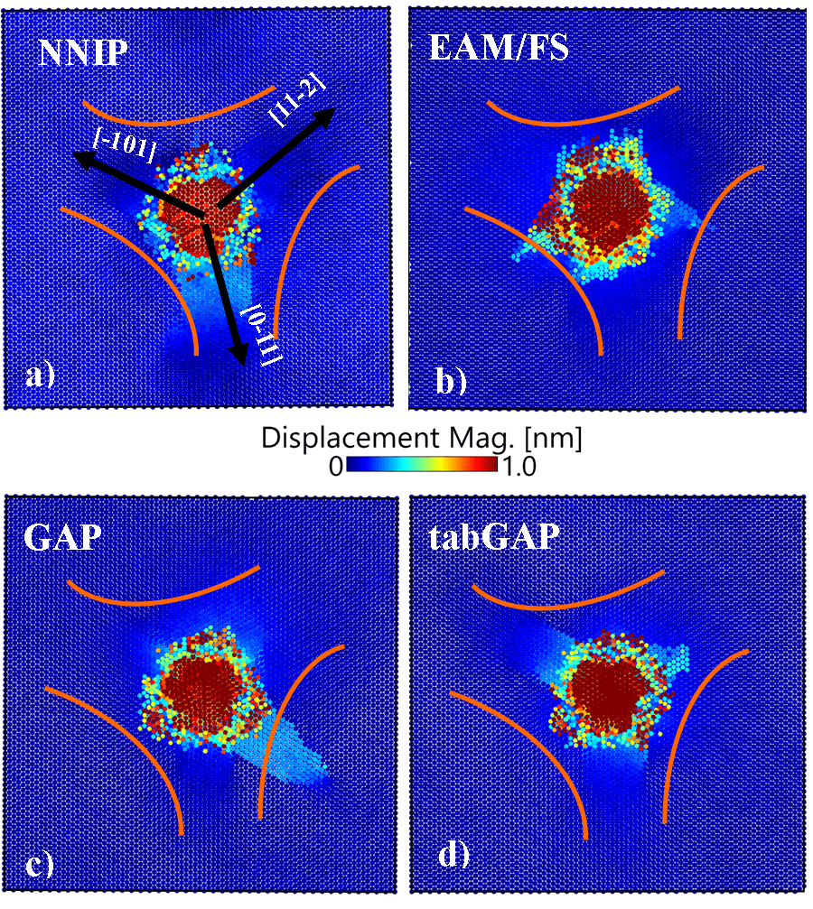
Figure 8: (Color online) Pileups and slip trace formations were observed on the $\{112\}$ and $\{011\}$ planes, as well as symmetric ones, for the [111] Mo samples using different methods: NNIP in (a), EAM/FS in (b), GAP in (c), and tabGAP in (d). In this analysis, we have included an orange line to emphasize the 3–fold rosette characteristic commonly seen in the indentation of BCC samples where NNIP simulations are capable to model it Domínguez-Gutiérrez et al. (2023); Varillas et al. (2017); Dominguez-Gutierrez et al. (2021).

IV Methods

IV.1 Descriptor parameters

In this work, PANNA: Properties from Artificial Neural Network Architectures Lot et al. (2020), which utilizes Tensorflow et al. (2015) to train/evaluate fully-connected feed-forward NNIPs, is used to develop the interatomic potential, with the modified version of Behler–Parrinello (mBP) descriptors Smith et al. (2017); Behler and Parrinello (2007). The mBP representation generates a fixed-size vector (the G-vector) for each atom in each configuration of the dataset. Each G-vector describes the environment of the corresponding atom of the configuration to which it belongs, up to a cutoff radius $R_{c}$. Although higher dimensional G-vectors lead to a more accurate representation of the target potential energy surface, oversized ones increase the MD simulation computational cost. In terms of the distances $R_{ij}$ and $R_{ik}$ of the atom $i$ from its neighbors $j$ and $k$ and the angle subtended by those distances $\theta_{ijk}$, the radial and angular G-vectors are given by:

$$G^{rad}_{i}[s]=\sum_{i\neq j}e^{-\eta(R_{ij}-R_{s})^{2}}f_{c}(R_{ij})$$ (1)

$$\begin{split}G^{ang}_{i}[s]&=2^{1-\zeta}\sum_{j,k\neq i}[1+cos(\theta_{ijk}-\theta_{s})]^{\zeta}\\ &\times e^{-\eta[\frac{1}{2}(R_{ij}+R_{ik})-R_{s}]^{2}}f_{c}(R_{ij})f_{c}(R_{ik})\end{split}$$ (2)

where the smooth cutoff function (which includes the cutoff radius $R_{c}$) is given by:

$$f_{c}(R_{ij})=\begin{cases}\frac{1}{2}\left[\cos\left(\frac{\pi R_{ij}}{R_{c}}\right)+1\right],&R_{ij}\leq R_{c}\\ 0,&R_{ij}>R_{c}\end{cases}$$ (3)

and $\eta$, $\zeta$, $\theta_{s}$ and $R_{s}$ are parameters, different for the radial and angular parts. Table. 2 shows all values selected for the descriptor parameters in this study. The choice of the cutoff value is made so that it covers up to three nearest neighbours of the center atom in the BCC Mo, which has a lattice constant of $a=3.17$ Å, and thus the third nearest neighbour’s distance is $a\times\sqrt{2}=4.48$ Å. The length of the G-vector for a single element system is

$$|G_{i}[s]|=(R_{s}^{ang}\times\theta_{s})+R_{s}^{rad},$$ (4)

which leads to a G-vector of length 152, given the parameters reported in Table. 2.

Descriptor parameter	Symbol	Value
Radial component:
Radial exponent (Å-2)	$\eta^{rad}$	$32$
cutoff (Å)	$R_{c}^{rad}$	$5$
Number of $R_{s}$ radial	$R_{s}^{rad}$	$24$
Angular component:
Radial exponent (Å-2)	$\eta^{ang}$	$16$
cutoff (Å)	$R_{c}^{ang}$	$5$
Number of $R_{s}$ angular	$R_{s}^{ang}$	$8$
Angular exponent	$\zeta$	$128$
Number of $\theta_{s}$	$\theta_{s}$	$16$

Table 2: Values of the parameters that appear in the definition of the radial and angular G-vectors, Eq.s(1), (2), (3). Where a number of components is given, the values are equispaced.

IV.2 Similarity measurements

In this study, a distance-based criterion is utilized to quantify the similarity between two distinct configurations. This criterion is subsequently extended to evaluate the closeness of two disparate datasets to one another. Consider two configurations, labeled as $\alpha$ and $\beta$, with $n$ and $m$ atoms per supercell, respectively. The distance matrix for the two configurations, $D^{\alpha\beta}$, has a $n\times m$ dimension and each element of the matrix is the eucleadian distance of atom $i$ in $\alpha$ to atom $j$ in $\beta$:

$$D^{\alpha\beta}_{i,j}=\lVert G^{\alpha}_{i}[s]-G^{\beta}_{j}[s]\rVert_{2}$$ (5)

Where $i$ $\in$ $\displaystyle\{1,2,\dots,n\}$ and $j$ $\in$ $\displaystyle\{1,2,\dots,m\}$, and each $G[s]$ is a 152 dimensional vector, as explained in the previous section. Given this matrix, we can compute the minimum distance of each atom $i$ in configuration $\alpha$ from any atom $j$ in configuration $\beta$, and we define the similarity measure from $\alpha$ to $\beta$ as the maximum among these minima, i.e.:

$$D^{\alpha\beta}=\max_{i}\min_{j}D^{\alpha\beta}_{i,j}.$$ (6)

It must be noted that this final quantity is not a proper distance, but a non-symmetric quantity giving us the “similarity measure” method, explained in this section, is subsequently employed to gain insights from the initial dataset. This also includes exploring ways to enhance the dataset through innovative configurations, specifically in relation to an indented supercell. For instance, one can compute the average of all $D^{\alpha\beta}$ values between atoms from two distinct datasets or configuration types within a dataset. This calculation provides an indication of the degree of (dis)similarity between considered datasets/configuration types. The same goes for measuring the similarity of a dataset to a targeted simulation, which in our case is an indented sample.

IV.3 Dataset evaluation and improvement

As a starting point, we used a dataset Byggmästar et al. (2020a) originally developed to train a MLFF within the GAP framework Bartók et al. (2010); Byggmästar et al. (2020b). The objective was to determine whether this dataset accurately represents the atomic configurations occurring during nanoindentation simulations, for which we employed an EAM potential Salonen et al. (2003). We then analyzed the obtained data to determine the degree of similarity between the atomic configurations in the dataset and those observed during the nanoindentation simulations.

Structure type	$N_{s}$	$N_{at}$	$N_{sel}$
Isolated atom	1	1	None
Dimer	19	2	None
Slice sample	1996	1	All
Distorted BCC	547	2	All
A15	100	8	None
C15	100	6	None
HCP	100	2	All
FCC	100	1	None
Diamond	100	2	None
Phonon	50	54	All
Self-interstitials (SIA)	32	121	14
di-Self-interstitials	14	122-252	All
Simple Cubic	100	1	None
Vacancy	210	53	All
di-Vacancy	10	118	All
tri-Vacancy	14	117	All
Liquid	45	128	None
Short range	90	53-55	None
Surface (100)	45	12	All
Surface (110)	45	12	All
Surface (111)	41	12	All
Surface (112)	45	12	All
Liquid Surface	24	128	All
$\gamma$-urface	178	12	All
GSFCs	100	18	All
GSFCs + SIA	100	55	All
Pileup	1000	32	All
HT + substrate	600	54-72	All

Table 3: The original dataset from Byggmästar et al. (2020a), showing $N_{s}$ as the number of structures, $N_{at}$ as the number of atoms per configuration, and $N_{sel}$ as the number of selected configurations in the final dataset.

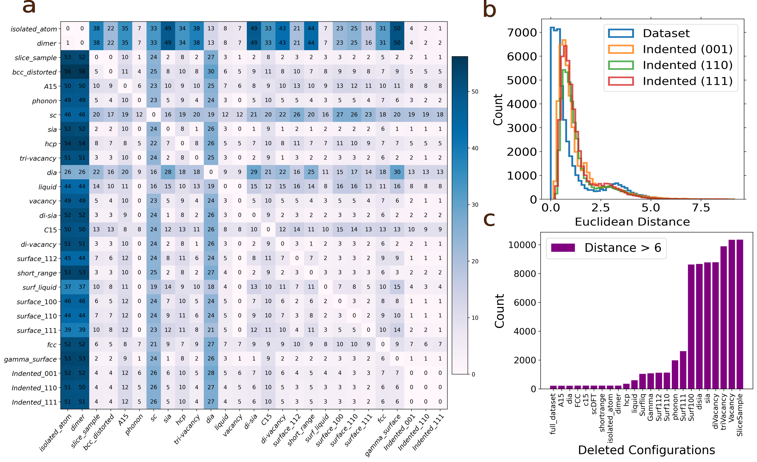
Figure 9: Dataset evaluation and stability. a) Average of minimum distances between different configuration types as well as with the indented samples. b) Distribution of the minimum distances of different configurations to the rest of the data points in the dataset and the minimum distances of the dataset with the indented configurations. c) Effect of configuration removal from the dataset on the minimum distances of the dataset to the indented sample.

This level of similarity is evaluated by identifying which atom $j$ in the dataset has the minimum distance to each atom $i$ in the indented sample. The obtained value corresponds to the largest minimum distance for each atom in the indented sample from all the atoms in the dataset. The concept of “distance” for two atoms $i$ and $j$, refers to the $l^{2}$-norm of $G_{i}[s]-G_{j}[s]$, where $G[s]$ are the fixed-size modified Behler-Parinnelo (mBP) descriptor vectors Smith et al. (2017); Behler and Parrinello (2007), as discussed in the previous sections. To this end, we compared the configuration types present in the dataset to those of all atoms identified in the indented sample and drew conclusions based on the level of correspondence between the two sets. Through this analysis, we aimed to gain insights into the suitability of the selected dataset for studying nanoindentation behavior and identifying the underlying mechanisms governing it.

To generate a suitable dataset for training a NNIP targeted at nanoindentation simulations, it is crucial to ensure that the configurations included accurately represent the three essential regions of a sample under indentation. These regions include the atoms on the surface of the sample, which correspond to the pileup patterns, the atoms situated beneath the indenter tip that undergo significant plastic deformation, and the atoms located on the nucleated dislocation cores. The evaluation of these three critical regions and development of configurations that closely resemble them can serve as a benchmark for ML potentials for other BCC materials.

Before comparing the original dataset with the indented sample, we calculated the average minimum distance between each pair of configuration types and generated a correlation figure to visualize their proximity (Fig. 9(a)). It is evident from this figure that although the isolated atom and dimer configurations are quite distant from almost all other configurations, they are relatively close to the indented samples. However, these configurations were not included in the final dataset due to their low numbers (1 and 19, respectively), which were deemed insufficient for training a NNIP. Moreover, the A15, simple cubic (sc), diamond (dia), liquid and C15 configurations were removed from the final dataset as they were located at a distance beyond the set threshold from the indented configurations, with simple cubic, diamond, and C15 configurations having the largest distance. Furthermore, we excluded short-range configurations from the final dataset because their energies varied significantly (Fig. S1(a)), leading to training difficulties. Finally, to reduce computational cost, we kept only half of the self-interstitial configurations in the final dataset. Table. 3 summarizes all modifications made to the original dataset.

Several methods can be employed to determine a “good” threshold for deciding whether to keep or remove a particular configuration from the dataset, based on its similarity to the indented configuration. In this study, we have chosen to use the start of the tail of the distribution of the minimum values in the dataset distance matrix as the threshold, which is approximately 6 based on Fig. 9(b). Fig. 9(b) also demonstrates that this value is consistent with the minimum distances between the dataset configurations and all three orientations of the indented samples. All decisions regarding whether to keep or remove a configuration from the final dataset in this study are based on this threshold.

To ensure the accuracy of the modifications made to the dataset, we removed one type of configuration from the dataset at a time and quantified the number of atoms in the indented samples that had minimum distances greater than 5 from the dataset (Fig. 9(c)). As our analysis shows, the number of atoms with a minimum distance greater than 5 to the dataset does not increase when A15, diamond, Face-Centered Cubic (FCC), simple cubic, short range, isolated atom, and dimer configurations are removed, indicating the dataset’s stability against the indented samples, whether these configurations are present in the dataset or not. However, upon removing Hexagonal Close-Packed (HCP) configurations, the number of atoms with a large distance from the dataset increases, which is consistent with the fact that the average minimum distance of HCP configurations to the indented samples is 5 . The greatest increase in the number of atoms with a distance greater than 5   from the dataset occurs when surface configurations are removed, which underscores their importance since they represent the surface in the nanoindentation simulations.

Following the modifications made to the dataset obtained from Byggmästar et al. (2020a), attempts were made to enhance its quality by incorporating various types of configurations and reevaluating the distances of the indented configuration from the dataset. Among the crucial local environments that should be included in the dataset are the atoms belonging to the dislocation cores. Furthermore, it was discovered that the distances of the atoms beneath the indenter tip and those on the surface exceeded the selected 6 threshold (Fig. 1(a)). These environments in the indented samples are critical to be covered in the dataset since dislocation cores play a vital role in the dislocation dynamics properties, and the atoms beneath the indenter tip trigger these line defects. Additionally, the plastic region beneath the surface is responsible for the pile-up patterns that appear on the surface of the indented configuration. It is also imperative to incorporate configurations in the dataset representing atoms on the surface to capture this phenomenon.

In order to model the aforementioned regions of an indented sample, we explored the use of high-temperature configurations to effectively reduce the distance between the atoms in these areas and the dataset, as depicted in Fig. 1(b). Nevertheless, accounting for the atoms beneath the indenter tip and on the surface requires the inclusion of a layer of frozen atoms in the high-temperature configurations that emulate the contact of the sample with the indenter tip. The addition of $1000$ isothermal-isobaric ensemble (NPT) high-temperature configurations with $16$ atoms in the $2\times 2\times 2$ supercells appeared to decrease the distances between the atoms on the dislocation cores and the dataset. We utilized the same approach for the atoms beneath the indenter tip. In this regard, we introduced $600$ configurations, denoted as “high temperature $+$ substrate”, where a layer of atoms was frozen while other atoms were heated to high temperatures (under the melting point). While there are various unique layers of atoms that can be taken into account as the contact to the substrate, we verified that 300 configurations ($3\times 3\times 3$) with $54$ atoms per supercell—displayed in the middle figure of Fig. 1-(b)—were adequate and most relevant after trying different layers of atoms. Additionally, we included 300 configurations ($4\times 3\times 3$) with $72$ atoms per supercell, which featured a layer of atoms frozen on top. Moreover, it is crucial for a NNIP’s dataset to incorporate configurations resembling the atoms located on the surface of the indented sample. To achieve this, we introduced $1000$ BCC surface configurations ($3\times 3\times 2$) with $32$ atoms per supercell, where a layer of atoms was frozen on top while the remaining atoms were subjected to high temperature. These configurations were named “pileup” in our study and enabled the dataset to account for the atoms in this region.

Another effective approach to cover the dislocation cores is through the use of GSFCs that incorporate a self-interstitial atom (SIA) atom on the surface (as illustrated in Fig. 2(a)). These configurations have been found to be particularly effective in reducing the distances of atoms on the dislocation cores from the dataset. While the use of GSFCs without an SIA on the surface can also reduce distances of atoms beneath the dislocation cores and on the slipping plane (as shown in Fig. 2(b)), it may not entirely cover all the atoms on the dislocation core.

Incorporating a SIA on the surface of the GSFCs leads to a significant decrease in the distances of almost all atoms on the dislocation cores from the dataset (as demonstrated in Fig. 2(c)). Notably, the use of GSFCs with a SIA instead of high-temperature configurations solely for the dislocation cores presents several advantages. For instance, the distribution of energies of these configurations is narrower, facilitating the learning process for the network (as depicted in Fig. S1(b)). Furthermore, only $100$ GSFCs with SIA configurations, as opposed to the $1000$ mentioned for high-temperature configurations, can ease the process of training the network. Additionally, using GSFCs with SIA configurations guarantees that no atoms on the dislocation core will have a distance greater than 6, thus ensuring the closeness of the distances of these configurations to the dislocation cores.

The visualization of the distances between the atoms in all three regions of interest and the dataset reveals a significant reduction in distances after incorporating the high-temperature configurations (see Fig. 1(c)). The distribution of distances for each region before and after adding the high-temperature configurations is depicted in Fig. 1(d). Although a few atoms still have distances greater than 6 under the indenter tip, the number of such atoms has notably decreased after adding the appropriate configurations. Finally, because we are trying to develop a NNIP for the case of nanoindentation simulation during which atoms are compressed under the indenter tip, we added $300$ compressed $3\times 3\times 4$ configurations with each of them including 72 atoms.

IV.4 DFT calculations

The DFT calculations were performed with the Quantum Espresso et al. (2009, 2017) (QE) package, using a norm-conserving PBEsol exchange-correlation functional Prandini et al. (2018); et al. (2016); Hamann (2013) and 14 valence electrons. The Brillouin zone was sampled using Monkhorst-Pack method Monkhorst and Pack (1976), and, from the convergence analysis of Fig. S2, the k-point mesh and plane-wave cutoff energy in a Mo unit-cell were set to $8\times 8\times 8$ and 60 $Ry$, respectively. The selected k-point grid was rescaled for supercells calculations according to their dimension, implying the use of a $2\times 2\times 2$ grid for $4\times 4\times 4$ conventional super-cells, and was set to $1\times 1\times 1$ for any bigger configuration. Smearing was introduced within the Methfessel-Paxton method Methfessel and Paxton (1989) to help convergence, with a spreading of 0.00735 $Ry$ (0.1 $eV$). The structural properties, involving elastic constants $C_{ij}$, Bulk modulus $B$ (in the Voigt-Reuss-Hill approximation Chung and Buessem (1967)) and Poisson ratio $\nu$, have been computed running the QE driver THERMO_PW the on a Mo unit-cell.

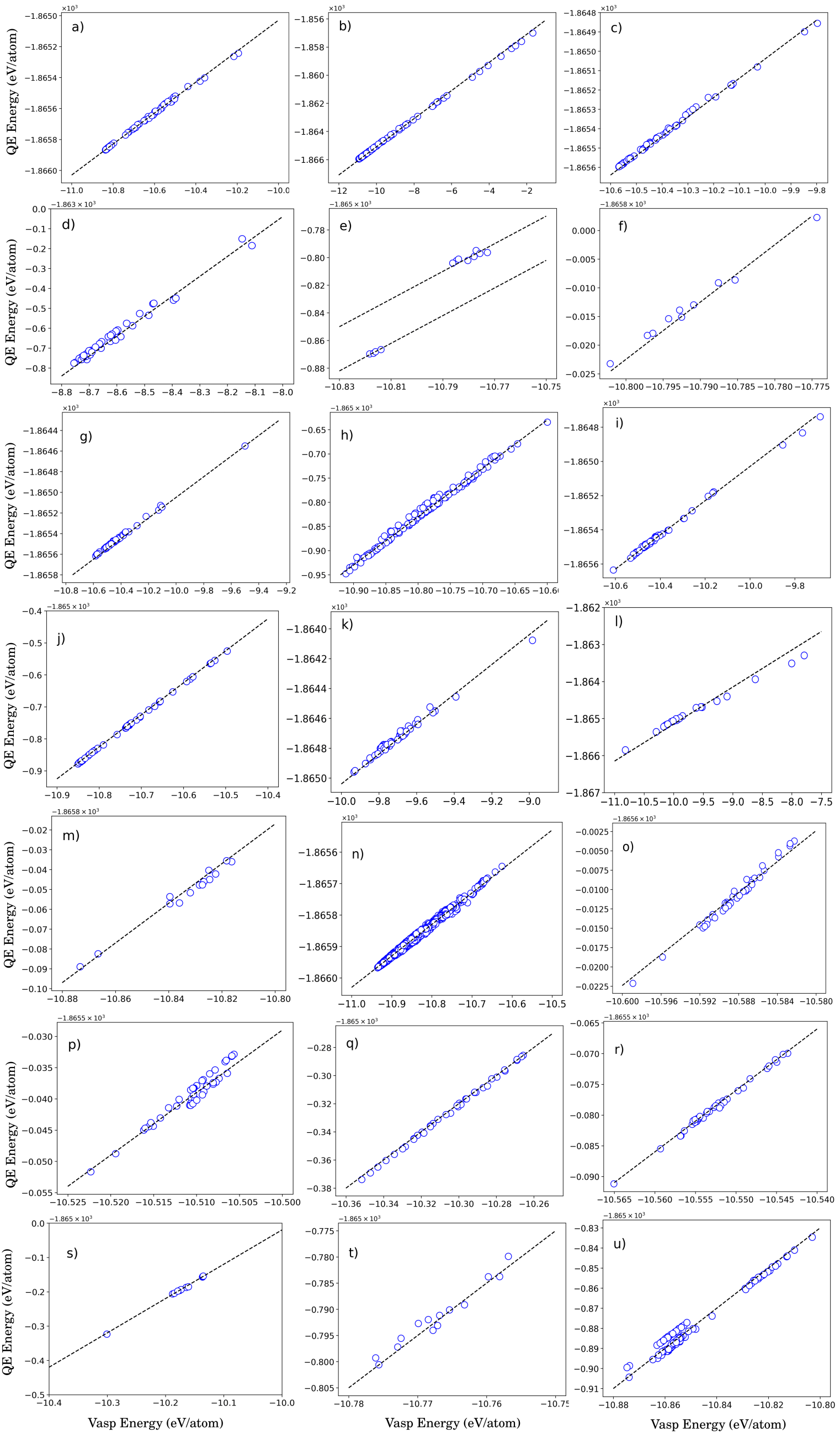
Figure S4: The total energies obtained in this work with Quantum Espresso (QE), compared to VASP (from the original GAP potential). The dashed lines represent a (y = x + b) function with y being the Quantum Espresso energy, x being the VASP energy and b is the y-intercept which is different for each panel and illustrates the correctness of the values we obtained from QE. Figures a) to u) are for the following configurations, respectively: A15, BCC, C15, diamond, di-sia, di-Vacancy, FCC, Gamma, HCP, phonon, sc, short range, sia, sliced sample, surface 100, surface 110, surface 111, surface 112, liquid surface, tri-Vacancy and vacancy.

The total energies of the configurations obtained from Byggmästar et al. (2020a) were compared with the values calculated in our work to make sure of their consistency, which is shown in Fig. S4.

IV.5 Neural Network Training

In the PANNA framework, the environmental descriptors of each atom are provided as input to a fully connected network with two hidden layers, consisting of 256 and 128 nodes for the first and second layers, respectively, both with Gaussian activation function, and a single-node output layer with linear activation. The atomic environment is represented by a descriptor with 152 components, resulting in a network with 71808 weights and 385 biases. A batch size of $10$ is utilized for training, while the model is trained using initial random weights and a constant learning rate of $10^{-4}$ throughout the training process. In this methodology, the energy of a configuration consisting of $N$ atoms is defined as the sum of atomic energy contributions:

$$E=\sum_{i=1}^{N}E_{i}(G_{i}),$$ (7)

where $E_{i}$ is the energy of atom $i$ with a G-vector of $G_{i}$. The force on atom $i$ which is situated at position $\vec{R}_{i}$ is given by:

$$\vec{F}_{i}=-\sum_{j}\sum_{\mu}\frac{\partial E_{j}}{\partial G_{j\mu}}\frac{\partial G_{j\mu}}{\partial\vec{R}_{i}}$$ (8)

with $j$ labeling the atoms located within the cutoff distance of atom $i$ and $\mu$ labeling the descriptor components.

To optimize the weights and bias parameters of the network, we use the Adam algorithm Kingma and Ba (2017) to compute gradients of randomly selected batches of the training dataset. The loss function for optimizing the network weights, denoted collectively as $W$, consists of two terms, one for the energy $\mathcal{L}_{E}(W)$, and one for the forces, $\mathcal{L}_{F}(W)$:

$$\mathcal{L}(W)=\mathcal{L}_{E}(W)+\mathcal{L}_{F}(W).$$ (9)

The energy contribution is given by:

$$\mathcal{L}_{E}(W)=\sum_{s\in{\rm batch}}\left[E_{s}^{{\rm DFT}}-E_{s}(W)\right]^{2}$$ (10)

where $s$ refers to the atomic configuration, $E_{s}^{DFT}$ is the total energy calculated from DFT (the target value) and $E_{s}(W)$ is the total energy predicted by the NNIP. The force contribution is given by:

$$\mathcal{L}_{F}(W)=\lambda_{F}\sum_{s\in{\rm batch}}\sum_{i=1}^{N_{s}}\left\lvert\vec{F}_{i;s}^{{\rm DFT}}-\vec{F}_{i;s}(W)\right\rvert^{2}$$ (11)

with $\vec{F}_{i;s}^{{\rm DFT}}$ the force obtained from DFT and $\vec{F}_{i;s}$ the force obtained from the NNIP, for atom $i$ in configuration $s$; $N_{s}$ is the total number of atoms in configuration $s$. The parameter $\lambda_{F}$ adjusts the relative contribution of the force component and was set to $\lambda_{F}=0.5$.

IV.6 Nanoindetation simulations

IV.6.1 Simulation method and parameters

To establish boundary conditions along the depth ($dz$) of the Mo samples, we divided them into three sections in the $z$ direction during the initial stage: a frozen section with a width of approximately 0.02$\times dz$, which ensured numerical cell stability; a thermostatic section about 0.08$\times dz$ above the frozen section, which dissipated heat generated during nanoindentation; and a dynamical atoms section, where the interaction with the indenter tip modified the surface structure of the samples. Furthermore, we included a 5 nm vacuum section at the top of the sample as an open boundary Kurpaska et al. (2022). We considered the indenter tip as a non-atomic repulsive imaginary (RI) rigid sphere and defined its force potential as

$$F(t)=K\left(\vec{r}(t)-R\right)^{2},$$ (12)

where $K=236$ eV/ų (37.8 GPa) was the force constant, and $\vec{r}(t)$ was the position of the center of the tip as a function of time, with a radius $R=3$ nm. We conducted molecular dynamics (MD) simulations using an NVE statistical thermodynamic ensemble and the velocity Verlet algorithm to emulate an experimental nanoindentation test. The $x$ and $y$ axes had periodic boundary conditions to simulate an infinite surface, while the $z$ orientation had a fixed bottom boundary and a free top boundary in all MD simulations Dominguez-Gutierrez et al. (2021); Domínguez-Gutiérrez et al. (2023).

In our simulations, we chose $\vec{r}(t)=x_{0}\hat{x}+y_{0}\hat{y}+(z_{0}\pm vt)\hat{z}$, where $x_{0}$ and $y_{0}$ were the center of the surface sample on the $xy$ plane, and $z_{0}=0.5$ nm was the initial gap between the surface and the indenter tip. The tip moved with a speed of $v=20$ m/s with a time step of $\Delta t=1$ fs. We chose the maximum indentation depth to be 2.0 nm to avoid the influence of boundary layers in the dynamical atoms region.

IV.6.2 Normalized maximum shear stress

The contact pressure, $P$, is calculated by using a linear elastic contact mechanics formulation Domínguez-Gutiérrez et al. (2023); Varillas et al. (2017):

$$P=2\pi\left[24p\left(\frac{E_{\rm Y}R}{1-\nu^{2}}\right)^{2}\right]^{1/3},$$ (13)

with $E_{Y}$ as the Young’s modulus, $p$ as the simulation load, $R$ the indenter radius, and $\nu$ the Poisson’s ratio; the radius of the contact area is obtained with the geometrical relationship:

$$\mathrm{a}(h)=\left[3PR\left(1-\nu^{2}\right)/8E_{\rm Y}\right]^{1/3}$$ (14)

which is related to the inner radius of the plastic region where the defects nucleate. This quantity provides an intrinsic measure of the surface resistance to a specific defect nucleation process Varillas et al. (2017); Domínguez-Gutiérrez et al. (2023). To determine the strength and stability of the Mo matrix under load, we compute the principal stress applied on the $z$ direction as Remington et al. (2014) :

$$\sigma_{zz}=-\mathcal{S}\left[\left(1-\frac{\arctan(\alpha)}{\alpha}\right)(1+\nu)-\frac{1}{2(1+1/\alpha^{2})}\right],$$ (15)

where the quantities $\mathcal{S}$ and $\alpha$ are defined as:

$$\mathcal{S}=\frac{3P_{\rm ave}}{2\pi\mathrm{a}(h)^{2}},\quad\alpha=\frac{\mathrm{a}(h)}{h}.$$

with $h$ as the indentation depth and $a(h)$ the contact area between the indenter tip and the top atomic layers. The stress applied in the direction parallel to the indenter surface is then expressed as:

$$\sigma_{xx}=\sigma_{yy}=-\frac{\mathcal{S}}{1+1/\alpha^{2}}$$ (16)

This gives the maximum shear stress:

$$\tau_{\rm max}=\frac{1}{2}\left(\sigma_{zz}-\sigma_{xx}\right),$$ (17)

that the material can withstand before it begins to undergo plastic deformation, being normalized by the applied pressure (equal to the applied force $F$ divided by the contact area). The normalized depth is the distance from the surface of the material to the point at which the maximum shear stress occurs, normalized by the radius of the indenter that is used to apply the shear forces.

IV.6.3 Defect analysis

In order to identify the defects in nanoindentation simulations, we apply the BCC Defect Analysis (BDA) developed by Möller and Biztek Möller and Bitzek (2016) which utilizes coordination number (CN), centrosymmetry parameter (CSP), and common neighbor analysis (CNA) techniques to detect typical defects found in bcc crystals. The characterization of the materials defects starts by calculating CN, CSP, and CNA values of all the atoms by considering a cutoff radius of $(1+\sqrt{2})/2a_{0}$ with $a_{0}$ as the lattice constant of Mo. Thus, the six next–nearest neighbors of perfect bcc atoms are into this cutoff and their CN value increases from 8 to 14. Consequently, BDA compares the CN and CSP values of each atom generating a list of non–bcc neighbors with CNA$\neq$bcc and CN$\neq$14 that classifies for the following typical defects: surfaces, vacancies, twin boundaries, screw dislocations, {110} planar faults, and edge dislocations.

Author Contributions

N.D.A. created and designed the DFT training dataset, performed all the NNIP training, compiled and analyzed the data, did NNIP-MD nanoindentation and GSFE simulations and wrote the manuscript. N.D.A. prepared all the figures, jointly with F.J.D. for the nanoindentation section. F.P. and E.Kü. supervised the training procedure and designed the similarity measurement method. F.J.D. supervised the nanoindentation part. D.M. did the DFT GSFE calculations and DFT validation of elastic properties with THERMO_PW. S.P. and E.K. supervised all aspects of the work. All authors contributed to revision of the manuscript.

ACKNOWLEDGEMENTS

We acknowledge support from the European Union Horizon 2020 Research and Innovation Programme under grant agreement no. 857470 and from the European Regional Development Fund via the Foundation for Polish Science International Research Agenda PLUS program grant No. MAB PLUS/2018/8. Computational resources were provided by the High Performance Cluster at the National Centre for Nuclear Research in Poland.

Competing Interests

The authors declare no competing interests.

V References

Supplementary Information for: Neural Network Interatomic Potentials For Open Surface Nanomechanics Applications

Amirhossein D. Naghdi^1,2,∗, Franco Pellegrini³, Emine Kücükbenli^4,5, Dario Massa^1,2, F. Javier Dominguez–Gutierrez¹, Efthimios Kaxiras^5,6, and Stefanos Papanikolaou^1,∗

¹NOMATEN Centre of Excellence, National Center for Nuclear Research, ul. A. Sołtana 7, 05-400 Swierk/Otwock

²IDEAS NCBR, ul. Chmielna 69, 00-801, Warsaw, Poland

³International School for Advanced Studies (SISSA), Via Bonomea, 265, I-34136 Trieste, Italy

⁴ Nvidia Corporation, Santa Clara, CA, USA

⁵ John A. Paulson School of Engineering and Applied Sciences, Harvard University, Cambridge, Massachusetts 02138, USA

⁶Department of Physics, Harvard University, Cambridge, Massachusetts 02138, USA

\begin{overpic}[width=195.12767pt]{Figs/ecut.png} \end{overpic}

\begin{overpic}[width=195.12767pt]{Figs/NK.png} \end{overpic}

Figure S2: DFT convergence check for a) cutoff energy and b k-point mesh grid.

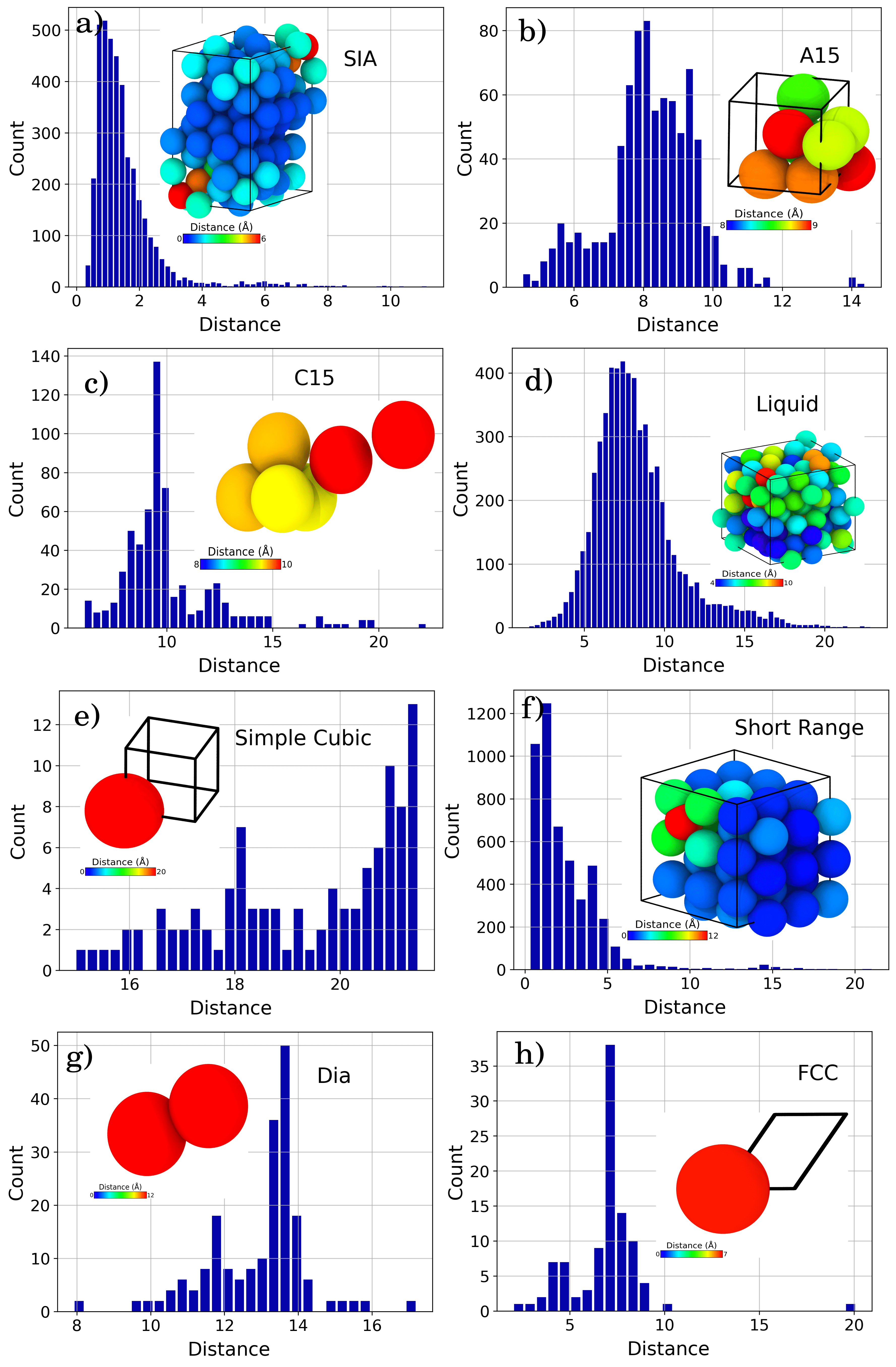
Figure S3: Distribution of minimum distances of each configuration to the indented sample for deleted configurations from the dataset. As it is shown in the insets, each configuration consists of number of atoms with large minimum distance.

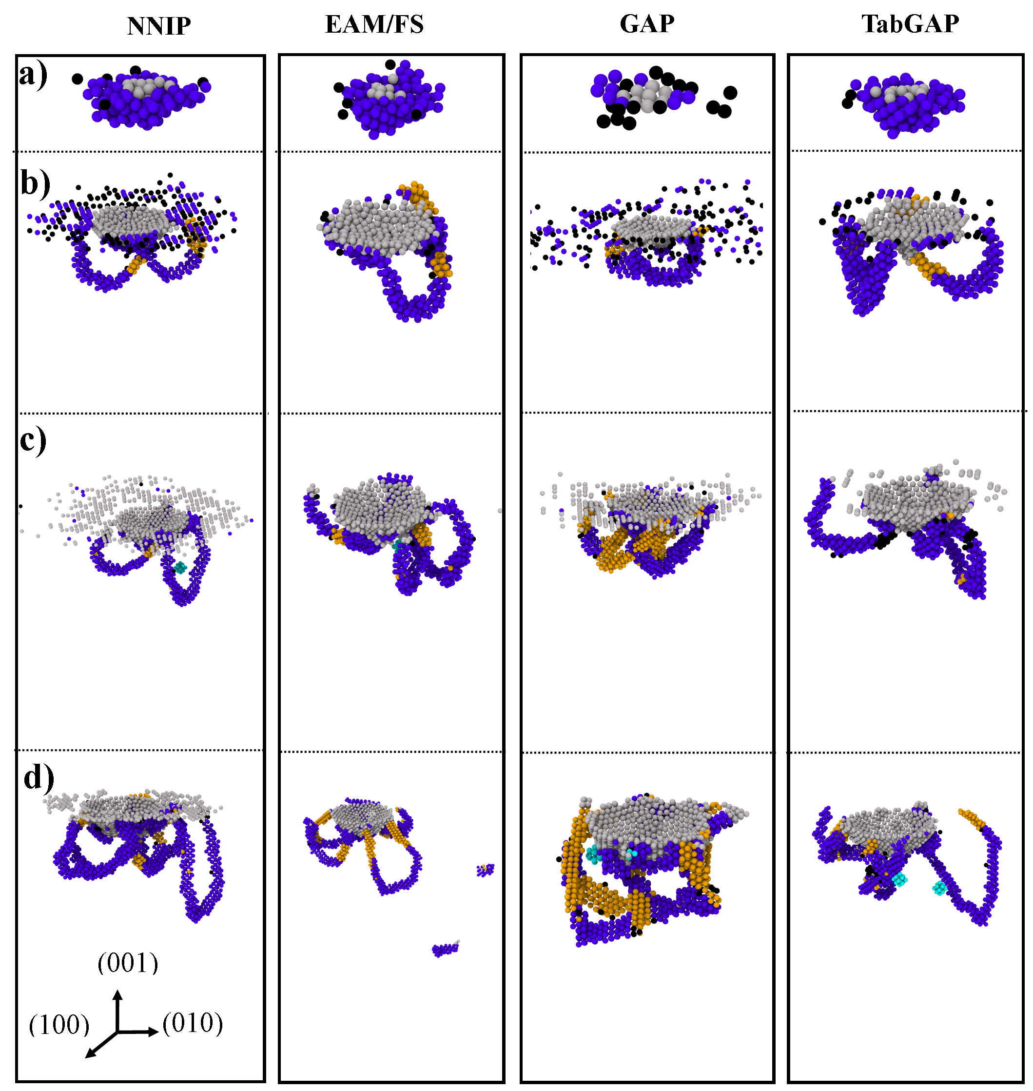
Figure S5: (Color online) Identified defects of indented (001) Mo sample by BDA method at different depths by NNIP, EAM, TabGAP, and GAP approaches. Material defects are depicted using different colors: gray spheres represent surface atoms in direct contact with the indenter tip, blue spheres indicate edge dislocations, light-blue spheres represent atoms in the vicinity of vacancies, yellow spheres depict twin/screw dislocations, and black spheres highlight unidentified defect atoms. The nucleation and propagation of edge dislocations on the {111} slip family are observed, which then evolve into prismatic loops. In addition, identified slip traces and pile-ups are well modeled by NNIP simulations showing the well–known three–fold symmetric rosette depths below 1.40 nm that are formed by [11$\bar{2}$], [$\bar{1}$01] and [0$\bar{1}$1] planes.

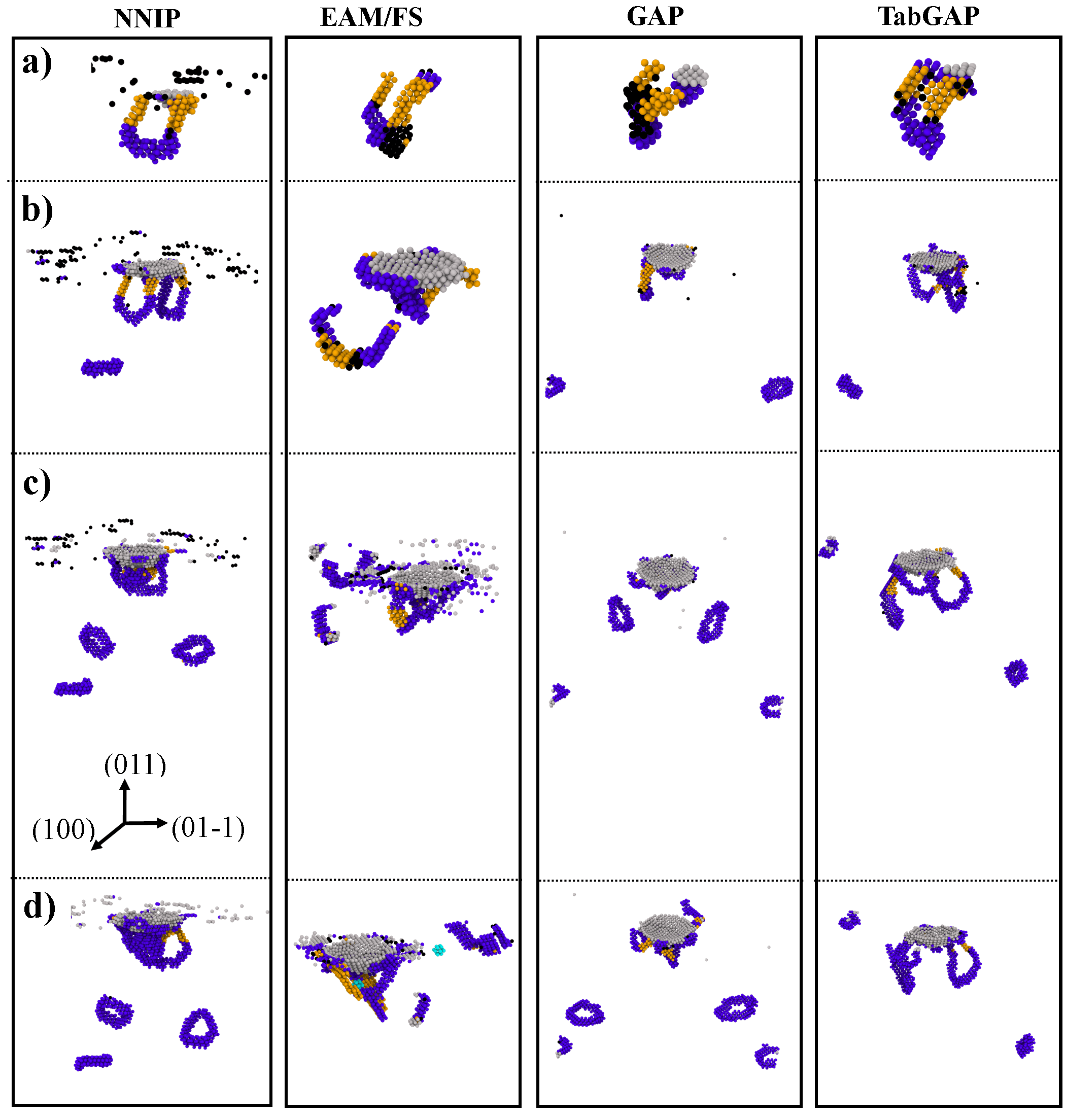
Figure S6: (Color online) Identified defects of indented (011) Mo sample by BDA method at different depths by NNIP, EAM, TabGAP, and GAP approaches. Material defects are depicted using different colors: gray spheres represent surface atoms in direct contact with the indenter tip, blue spheres indicate edge dislocations, light-blue spheres represent atoms in the vicinity of vacancies, yellow spheres depict twin/screw dislocations, and black spheres highlight unidentified defect atoms. The nucleation and propagation of edge dislocations on the {111} slip family are observed, which then evolve into prismatic loops. In addition, identified slip traces and pile-ups are well modeled by NNIP simulations showing the well–known three–fold symmetric rosette depths below 1.40 nm that are formed by [11$\bar{2}$], [$\bar{1}$01] and [0$\bar{1}$1] planes.

References

- Kim and Greer (2009) J.-Y. Kim and J. R. Greer, Acta Materialia 57, 5245 (2009).
- Kim et al. (2012) J.-Y. Kim, D. Jang, and J. R. Greer, International Journal of Plasticity 28, 46 (2012).
- Motamedi et al. (2020) M. Motamedi, A. Naghdi, and S. Jalali, Proceedings of the Institution of Mechanical Engineers, Part C: Journal of Mechanical Engineering Science 234, 635 (2020), https://doi.org/10.1177/0954406219878760 .
- Schuh (2006) C. A. Schuh, Materials Today 9, 32 (2006).
- Varillas et al. (2017) J. Varillas, J. Ocenasek, J. Torner, and J. Alcala, Acta Materialia 125, 431 (2017).
- Kurpaska et al. (2022) L. Kurpaska, F. Dominguez-Gutierrez, Y. Zhang, K. Mulewska, H. Bei, W. Weber, A. Kosińska, W. Chrominski, I. Jozwik, R. Alvarez-Donado, S. Papanikolaou, J. Jagielski, and M. Alava, Materials & Design 217, 110639 (2022).
- Pathak and Kalidindi (2015) S. Pathak and S. R. Kalidindi, Materials Science and Engineering: R: Reports 91, 1 (2015).
- Voyiadjis and Yaghoobi (2017) G. Z. Voyiadjis and M. Yaghoobi, Crystals 7, 321 (2017).
- Remington et al. (2014) T. Remington, C. Ruestes, E. Bringa, B. Remington, C. Lu, B. Kad, and M. Meyers, Acta Materialia 78, 378 (2014).
- Gagel et al. (2016) J. Gagel, D. Weygand, and P. Gumbsch, Acta Materialia 111, 399 (2016).
- Naghdi et al. (2022) A. Naghdi, F. J. Dominguez-Gutierrez, W. Y. Huo, K. Karimi, and S. Papanikolaou, “Dynamic nanoindentation and short-range order in equiatomic nicocr medium entropy alloy lead to novel density wave ordering,” (2022), arXiv:2211.05436 [cond-mat.mtrl-sci] .
- Taneike et al. (2003) M. Taneike, F. Abe, and K. Sawada, Nature 424, 294 (2003).
- Haque and Saif (2002) M. A. Haque and M. T. A. Saif, Experimental Mechanics 42, 123 (2002).
- De Hosson et al. (2006) J. T. M. De Hosson, W. A. Soer, A. M. Minor, Z. Shan, E. A. Stach, S. A. Syed Asif, and O. L. Warren, Journal of Materials Science 41, 7704 (2006).
- Durst et al. (2005) K. Durst, B. Backes, and M. Göken, Scripta Materialia 52, 1093 (2005).
- Maier-Kiener et al. (2017) Maier-Kiener, Verena, Durst, and Karsten, JOM 69, 2246 (2017).
- Casals et al. (2007) O. Casals, J. Očenašek, and J. Alcala, Acta Materialia 55, 55 (2007).
- Smith et al. (2003) R. Smith, D. Christopher, S. D. Kenny, A. Richter, and B. Wolf, Phys. Rev. B 67, 245405 (2003).
- Swaddiwudhipong et al. (2006) S. Swaddiwudhipong, K. Tho, J. Hua, and Z. Liu, International Journal of Solids and Structures 43, 1117 (2006).
- Dominguez-Gutierrez et al. (2021) F. Dominguez-Gutierrez, S. Papanikolaou, A. Esfandiarpour, P. Sobkowicz, and M. Alava, Materials Science and Engineering: A 826, 141912 (2021).
- Kramer et al. (2001) D. Kramer, K. Yoder, and W. Gerberich, Philosophical Magazine A-physics of Condensed Matter Structure Defects and Mechanical Properties - PHIL MAG A 81, 2033 (2001).
- Biener et al. (2007) M. M. Biener, J. Biener, A. M. Hodge, and A. V. Hamza, Phys. Rev. B 76, 165422 (2007).
- Voyiadjis and Faghihi (2012) G. Z. Voyiadjis and D. Faghihi, Procedia IUTAM 3, 205 (2012), iUTAM Symposium on Linking Scales in Computations: From Microstructure to Macro-scale Properties.
- Plummer (2019) K. P. E. Plummer, University of Oxford (2019).
- Frydrych et al. (2023) K. Frydrych, F. Dominguez-Gutierrez, M. Alava, and S. Papanikolaou, Mechanics of Materials 181, 104644 (2023).
- Knapp et al. (1999) J. A. Knapp, D. M. Follstaedt, S. M. Myers, J. C. Barbour, and T. A. Friedmann, Journal of Applied Physics 85, 1460 (1999), https://pubs.aip.org/aip/jap/article-pdf/85/3/1460/10597542/1460_1_online.pdf .
- Lichinchi et al. (1998) M. Lichinchi, C. Lenardi, J. Haupt, and R. Vitali, Thin Solid Films 312, 240 (1998).
- Zhou et al. (2010) C. Zhou, S. B. Biner, and R. LeSar, Acta Materialia 58, 1565 (2010).
- Motz et al. (2008) C. Motz, D. Weygand, J. Senger, and P. Gumbsch, Acta Materialia 56, 1942 (2008).
- Song et al. (2019) H. Song, H. Yavas, E. V. der Giessen, and S. Papanikolaou, Journal of the Mechanics and Physics of Solids 123, 332 (2019), the N.A. Fleck 60th Anniversary Volume.
- Xu et al. (2024) Q. Xu, A. Zaborowska, K. Mulewska, W. Huo, K. Karimi, F. J. Domínguez-Gutiérrez, Łukasz Kurpaska, M. J. Alava, and S. Papanikolaou, Vacuum 219, 112733 (2024).
- Domínguez-Gutiérrez et al. (2023) F. J. Domínguez-Gutiérrez, P. Grigorev, A. Naghdi, J. Byggmästar, G. Y. Wei, T. D. Swinburne, S. Papanikolaou, and M. J. Alava, Phys. Rev. Mater. 7, 043603 (2023).
- Naghdi et al. (2023) A. H. Naghdi, K. Karimi, A. E. Poisvert, A. Esfandiarpour, R. Alvarez, P. Sobkowicz, M. Alava, and S. Papanikolaou, Phys. Rev. B 107, 094109 (2023).
- Karimi et al. (2023) K. Karimi, A. Esfandiarpour, and S. Papanikolaou, “Serrated plastic flow in slowly-deforming complex concentrated alloys: universal signatures of dislocation avalanches,” (2023), arXiv:2310.03828 [cond-mat.mtrl-sci] .
- Karimi and Papanikolaou (2023) K. Karimi and S. Papanikolaou, “Tuning brittleness in multi-component metallic glasses through chemical disorder aging,” (2023), arXiv:2309.11867 [cond-mat.soft] .
- Behler and Parrinello (2007) J. Behler and M. Parrinello, Phys. Rev. Lett. 98, 146401 (2007).
- Bartók et al. (2010) A. P. Bartók, M. C. Payne, R. Kondor, and G. Csányi, Phys. Rev. Lett. 104, 136403 (2010).
- Thompson et al. (2015) A. Thompson, L. Swiler, C. Trott, S. Foiles, and G. Tucker, Journal of Computational Physics 285, 316 (2015).
- Shapeev (2016) A. V. Shapeev, Multiscale Modeling & Simulation 14, 1153 (2016), https://doi.org/10.1137/15M1054183 .
- Glielmo et al. (2018) A. Glielmo, C. Zeni, and A. De Vita, Phys. Rev. B 97, 184307 (2018).
- Zhang et al. (2018) L. Zhang, J. Han, H. Wang, R. Car, and W. E, Phys. Rev. Lett. 120, 143001 (2018).
- Behler (2016) J. Behler, The Journal of Chemical Physics 145, 170901 (2016), https://doi.org/10.1063/1.4966192 .
- Shaidu et al. (2021) Y. Shaidu, E. Küçükbenli, R. Lot, F. Pellegrini, E. Kaxiras, and S. de Gironcoli, npj Computational Materials 7, 52 (2021).
- Li et al. (2021) Q.-J. Li, E. Küçükbenli, S. Lam, B. Khaykovich, E. Kaxiras, and J. Li, Cell Reports Physical Science 2, 100359 (2021).
- Byggmästar et al. (2022) J. Byggmästar, K. Nordlund, and F. Djurabekova, Phys. Rev. Mater. 6, 083801 (2022).
- Vandermause et al. (2020) J. Vandermause, S. B. Torrisi, S. Batzner, Y. Xie, L. Sun, A. M. Kolpak, and B. Kozinsky, npj Computational Materials 6, 20 (2020).
- Pellegrini et al. (2023) F. Pellegrini, R. Lot, Y. Shaidu, and E. Küçükbenli, “Panna 2.0: Efficient neural network interatomic potentials and new architectures,” (2023), arXiv:2305.11805 [physics.comp-ph] .
- Musaelian et al. (2023) A. Musaelian, S. Batzner, A. Johansson, L. Sun, C. J. Owen, M. Kornbluth, and B. Kozinsky, Nature Communications 14, 579 (2023).
- Batatia et al. (2022) I. Batatia, S. Batzner, D. P. Kovács, A. Musaelian, G. N. C. Simm, R. Drautz, C. Ortner, B. Kozinsky, and G. Csányi, “The design space of e(3)-equivariant atom-centered interatomic potentials,” (2022), arXiv:2205.06643 .
- Owen et al. (2023a) C. J. Owen, Y. Xie, A. Johansson, L. Sun, and B. Kozinsky, “Stability, mechanisms and kinetics of emergence of au surface reconstructions using bayesian force fields,” (2023a), arXiv:2308.07311 [cond-mat.mtrl-sci] .
- Owen et al. (2023b) C. J. Owen, N. Marcella, Y. Xie, J. Vandermause, A. I. Frenkel, R. G. Nuzzo, and B. Kozinsky, “Unraveling the catalytic effect of hydrogen adsorption on pt nanoparticle shape-change,” (2023b), arXiv:2306.00901 [cond-mat.mtrl-sci] .
- Goryaeva et al. (2021) A. M. Goryaeva, J. Dérès, C. Lapointe, P. Grigorev, T. D. Swinburne, J. R. Kermode, L. Ventelon, J. Baima, and M.-C. Marinica, Phys. Rev. Mater. 5, 103803 (2021).
- Byggmästar et al. (2019) J. Byggmästar, A. Hamedani, K. Nordlund, and F. Djurabekova, Phys. Rev. B 100, 144105 (2019).
- Nikoulis et al. (2021) G. Nikoulis, J. Byggmästar, J. Kioseoglou, K. Nordlund, and F. Djurabekova, Journal of Physics: Condensed Matter 33, 315403 (2021).
- Byggmästar et al. (2021) J. Byggmästar, K. Nordlund, and F. Djurabekova, Phys. Rev. B 104, 104101 (2021).
- Byggmästar et al. (2020a) J. Byggmästar, K. Nordlund, and F. Djurabekova, Phys. Rev. Materials 4, 093802 (2020a).
- Lot et al. (2020) R. Lot, F. Pellegrini, Y. Shaidu, and E. Küçükbenli, Computer Physics Communications 256, 107402 (2020).
- Salonen et al. (2003) E. Salonen, T. Järvi, K. Nordlund, and J. Keinonen, Journal of Physics: Condensed Matter 15, 5845 (2003).
- Smith et al. (2017) J. S. Smith, O. Isayev, and A. E. Roitberg, Chem. Sci. 8, 3192 (2017).
- Rumble (2019) J. Rumble, CRC Handbook of Chemistry and Physics, 100th Edition, 100th ed. (CRC Press, Boca Raton, FL, 2019).
- Möller and Bitzek (2016) J. J. Möller and E. Bitzek, MethodsX 3, 279 (2016).
- Mulewska et al. (2023) K. Mulewska, F. Dominguez-Gutierrez, D. Kalita, J. ByggmAstar, G. Wei, W. Chromiński, S. Papanikolaou, M. Alava, L. Kurpaska, and J. Jagielski, Journal of Nuclear Materials 586, 154690 (2023).
- et al. (2015) M. A. et al., “TensorFlow: Large-scale machine learning on heterogeneous systems,” (2015), software available from tensorflow.org.
- Byggmästar et al. (2020b) J. Byggmästar, K. Nordlund, and F. Djurabekova, Phys. Rev. Mater. 4, 093802 (2020b).
- et al. (2009) P. G. et al., Journal of Physics: Condensed Matter 21, 395502 (2009).
- et al. (2017) P. G. et al., Journal of Physics: Condensed Matter 29, 465901 (2017).
- Prandini et al. (2018) G. Prandini, A. Marrazzo, I. E. Castelli, N. Mounet, and N. Marzari, npj Computational Materials 4, 72 (2018).
- et al. (2016) K. L. et al., Science 351, aad3000 (2016), https://www.science.org/doi/pdf/10.1126/science.aad3000 .
- Hamann (2013) D. R. Hamann, Phys. Rev. B 88, 085117 (2013).
- Monkhorst and Pack (1976) H. J. Monkhorst and J. D. Pack, Phys. Rev. B 13, 5188 (1976).
- Methfessel and Paxton (1989) M. Methfessel and A. T. Paxton, Phys. Rev. B 40, 3616 (1989).
- Chung and Buessem (1967) D. Chung and W. Buessem, Journal of Applied Physics 38, 2535 (1967).
- (73) “Thermo_pw driver for qe (github link).” .
- Kingma and Ba (2017) D. P. Kingma and J. Ba, “Adam: A method for stochastic optimization,” (2017), arXiv:1412.6980 [cs.LG] .