Tangency as a limit of transverse intersections

Abstract.

We interpret tangency as a limit of two transverse intersections. Using this approach, we obtain a concrete formula to enumerate smooth degree $d$ plane curves tangent to a given line at multiple points with arbitrary order of tangency. Then one nodal curves with multiple tangencies of any order are enumerated. Finally, the plane curves with one cusp that are tangent to first order to a given line at multiple points are enumerated. Also a new way to enumerate curves with one node is given. We extend that method to enumerate curves with two nodes and then go on to enumerate curves with one tacnode; the latter is interpreted as a limit of the former. In the last part of the paper, we show how this idea can be applied in the setting of stable maps and perform a concrete computation to enumerate rational curves with first order tangency. A large number of low degree cases have been worked out explicitly.

1. Introduction

A prototypical question in enumerative geometry is as follows: what is the characteristic number of curves in a linear system that have certain prescribed singularities and are tangent to a given divisor of various orders at multiple points? The curves are, of course, required to meet further insertion conditions so that the ultimate answer is a finite number. For example, in $\mathbb{CP}^{2}$ there are exactly $2$ conics passing through $4$ generic points that are tangent to a given line, and there are $36$ nodal cubics in $\mathbb{CP}^{2}$ through $7$ generic points tangent to a given line. These are some special cases of the famous Caporaso-Harris formula, [3], which addresses the following question: How many degree $d$ curves are there in $\mathbb{CP}^{2}$ that pass through $\mathsf{g}$ generic points, having $\delta$ nodes that are tangent to a given line at $r$ distinct points, with the orders of tangency being $k_{1},\,k_{2},\,\cdots,\,k_{r}$, where

$$\mathsf{g}\,\,:=\,\,\frac{d(d+3)}{2}-\big{(}\delta+(k_{1}+k_{2}+\ldots+k_{r})\big{)}.$$

A key insight of Caporaso-Harris is a degeneration argument. They argue that the characteristic number of degree $d$ plane curves, passing through $\mathsf{g}$ generic points, coincides with the characteristic number of plane curves through $\mathsf{g}-1$ generic points and one point on a given line, plus an excess contribution coming from curves of lower degree. This degeneration argument helps them to formulate the number of degree $d$ plane curves with prescribed tangencies in terms of counts of plane curves of lower degree (but possibly with higher order tangencies).

The purpose of this paper is to give a new way to think about the question of tangency. This can be applied to approach questions studied in [3], i.e., counting curves in a linear system. But unlike the Caporaso-Harris formula — which counts curves with only nodal singularities — we will be counting curves with degenerate singularities as well.

2. A picture

The main idea of this paper can be summarized in one picture:

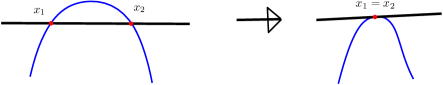
Figure 1. Tangency as a limit of transverse intersection

Let us briefly explain what this cryptic remark means. The right hand side of Figure 1 shows a curve tangent to a given line. Conventional wisdom suggests that we should view the tangency condition in the following way: the directional derivative of the function, defining the curve, along the direction of the line is zero. This approach is taken by the fourth author in [13] and [14]. In this paper, we adopt the following perspective: View tangency as a condition when two points collide as shown in the left hand side of Figure 1. This point of view makes it possible to enumerate curves with tangencies.

One can also study the question of enumerating stable maps tangent to a given divisor. The analogue of the first approach described in the previous paragraph is this: View tangency as the differential of the stable map vanishing in the normal direction to the divisor. This approach has been taken by Andreas Gathmann in [7], [8] and [9], where he successfully enumerates rational curves tangent to a given divisor.

The idea of interpreting tangency as a limit of transverse points has appeared in the literature in the context of stable maps. It has actually been discussed by Gathmann in his paper [6, p. 41]. Subsequently, this idea has also been discussed in the more recent paper by Dusa McDuff and Kyler Siegel [12, pp. 1179–1180]. The discussion in [12] illustrates that for applying this idea in the context of stable maps to enumerate curves with tangencies, we will need to compute the characteristic number of curves with an $m$-fold point; [2] precisely does the latter. Hence, using the results of [2] and by interpreting tangency as a limit of points lying on a line (as illustrated by Figure 1), it is possible to enumerate stable maps with tangencies. In Section 9, a very concrete computation based on this idea is worked out.

Finally, in Section 9.3 this idea is pursued again, but with a difference. We make the points in the domain come together, not in the image. This directly gives us rational curves with tangencies. The idea is implemented using the WDVV equation (namely, the equality of divisors in $\overline{M}_{0,4}$).

2.1. Organization of the paper

Section 3 outlines the underlying geometric behaviour of our results, avoiding technicalities, in particular, the results are presented with the help of rough pictures and are given intuitive geometric justifications. In Section 4 we state and prove a very simple looking lemma that will form a central part of the paper. This lemma will be called the collision lemma.
          In Sections 5, 6 and 7 all the main results of the paper are stated and proved. In particular, Section 5 presents the result to count smooth curves with tangencies at multiple points (see Theorems 5.2 and 5.3). Section 6 examines the enumeration of one nodal curve with multiple tangencies at multiple points (see Theorems 6.3, 6.4, 6.5, 6.6 and 6.7). In Section 7, we examine one cuspidal curve with multiple tangencies of first order (see Theorems 7.2, 7.4 and 7.6). Next, in Section 8, we give a new way to enumerate plane curves with certain singularities. In Section 9 we enumerate rational curves with first order tangency.

Finally, in Section 10, we perform explicit computations and verify special cases of the results using other known results. We have written a mathematica program to implement the formulas in Sections 5, 6, 7, 8 and 9. We have also written a Python program to implement the Caporaso-Harris formula. The programs are available in the web page

$$\textnormal{\url{https://www.sites.google.com/site/ritwik371/home}}.$$

The reader is invited to use the program and verify the assertions.

2.2. Further remarks

One particular aspect of our formula is as follows. We do not insist on keeping the line fixed and then look at curves tangent to that line. For example, suppose we wish to enumerate curves tangent to a given line to second order. Our result will immediately answer the following question: How many pairs, consisting of a line and a degree $d$ curve, are there such that the line passes through $m$ points and the curve passes through $n$ points and is tangent to the line to second order, where $m+n\,=\,\frac{d(d+3)}{2}$. The special case of $m\,=\,2$ is when the line is fixed.

The other point is as follows. When we are enumerating singular curves, it is not necessary for the singularity to be free; it can be constrained to lie on a cycle. For example, we can directly answer the following question: How many nodal degree $d$ curves are there tangent to a given line, such that the nodal point lies on the intersection of $m$ lines and the curve passes through $n$ points, where $m+n\,=\,\frac{d(d+3)}{2}-2$. The special case of $m\,=\,0$ corresponds to the nodal point being free. The case $m\,=\,1$ corresponds to the nodal point lying on a line. Similarly, $m\,=\,2$ corresponds to the nodal point lying on a fixed point. The number is obviously zero if $m$ is greater than $2$. We can also answer a more general question by allowing the line to vary as well.

It may be mentioned that neither of these two generalizations, namely varying the line or imposing a further constraint on the singular point, are covered by the Caporaso-Harris formula.

3. Geometric viewpoints of the results

3.1. A way to think about tangencies

3.1.1. Smooth curves with tangencies

Consider the space of degree $d$ curves in $\mathbb{CP}^{2}$. This is a complex projective space of dimension

$$\delta_{d}\,\,:=\,\,\frac{d(d+3)}{2}.$$ (3.1)

A question: How many degree $d$ curves are there in $\mathbb{CP}^{2}$ passing through $\delta_{d}-1$ generic points, that are tangent to a given line? This question leads to the space of curves and a point $x$, such that $x$ lies on both the line and the curve. We then observe that being tangent to the line at the point $x$ is equivalent to the condition that the directional derivative of the curve along the line vanishes (at the point $x$). This condition can be interpreted as a condition for being a section of a certain vector bundle. When $d$ is sufficiently large, this section will be transverse to the zero section of the vector bundle, and hence the Euler class of the bundle in question will give the desired number.

Let us now move one step ahead and ask the following question: How many degree $d$ curves are there in $\mathbb{CP}^{2}$ passing through $\delta_{d}-2$ generic points, that are tangent to a given line at two distinct points? This leads to the space of curves with two marked points $x_{1}$ and $x_{2}$, such that the curve is tangent to the line at $x_{1}$ while the point $x_{2}$ lies on both the line and the curve. A pictorial description of such a curve:

While it may be hoped that the Euler class of the relevant vector bundle will give the desired answer, this actually turns out to be untrue: the reason being that there is a degenerate contribution to the Euler class. This degeneracy occurs when the points $x_{1}$ and $x_{2}$ become equal producing the following object:

Note that the resulting curve in the closure is tangent to the given line of order two.

Let us now give an alternative way to enumerate curves with tangencies. Instead of interpreting tangency as the vanishing of a certain derivative, think of it in the following way: First, consider the space of curves with two marked points $x_{1}$ and $x_{2}$, such that both the points lie on the curve and the line. Now impose the condition that $x_{1}$ becomes equal to $x_{2}$. This will give the space of curves tangent to a given line because the curve will be tangent to this line precisely when the two points $x_{1}$ and $x_{2}$ collide and become equal. This can be visualized through the following picture:

3.1.2. Unisingular curves with tangencies

Consider the following question: How many degree $d$ plane curves are there through $\delta_{d}-2$ (see (3.1)) generic points that are tangent to a given line while possessing a node? For this, consider the space of curves with three points $p_{1}$, $x_{1}$, and $x_{2}$ such that the curve has a node at $p_{1}$ and intersects the given line at $x_{1}$ and $x_{2}$. Next, impose the condition that $x_{1}$ becomes equal to $x_{2}$. We might naively expect that this will give us precisely the space of one nodal curves tangent to a given line, as it would be suggested by the following picture:

But there is an extra object that occurs. There is also the space of curves with one node lying on the line, as shown by the following picture:

This ensues a degenerate contribution to the Euler class. The same thing happens if the curve has a more degenerate singularity. We have been able to compute the degenerate contribution to the Euler class in the following cases:

• When the degree $d$ plane curve has a node and is tangent to a given line at multiple points of any order.

• When the degree $d$ plane curve has a cusp and is tangent to a given line at multiple points (only tangency of order one).

When the singularity is a node, our answers agree with those predicted by the Caporaso-Harris formula.

There is actually no need to stop at one singular point. As an example, suppose we want to compute the characteristic number of curves with two nodes that are tangent to a given line at two points — both to first order. We can proceed as before by replacing one of the tangency point as two transverse points and then requiring them to collide. What will eventually be required is to compute the characteristic number of curves with two nodes both lying on a line.

3.2. A way to think about singularities

3.2.1. Nodal curves

Consider the following question: How many degree $d$ curves are there in $\mathbb{CP}^{2}$ that pass through $\delta_{d}-1$ (see (3.1)) generic points and have a node? Let us start by reviewing the traditional approach to solve this question. Consider the space of curves and a point in $\mathbb{CP}^{2}$, such that the point lies on the curve. On this space, impose the condition that the total derivative of curve evaluated at the point is zero. The vanishing of this derivative is interpreted as the Euler class of a suitable bundle, which gives the desired number.

We now describe a new way to solve this same question. Begin with a slightly different question: How many degree $d$ curves are there in $\mathbb{CP}^{2}$ that pass through $\delta_{d}-2$ generic points and possessing a node on a given line? First consider the space of curves with a marked point $p$ at which the curve is tangent to the line. It was explained in Section 3.1 a way to think of this space. On this space impose the condition that the derivative of the curve in the normal direction vanishes. That precisely means that the curve has a node at $p$.

Hence, computation of the Euler class of the relevant bundle will yield the desired number.

It might seem that we have solved a question different from the original one, where the node was not required to lie on the given line. That is not at all the case. Consider a more general question. Instead of counting nodal curves, where the node lies on a fixed line, let us count pairs: a line and a curve, together with a marked point, such that the point lies on both the line and the curve while the curve has a node at that point. Now impose the condition that the line passes through $m$ points and the curve passes through $n$ points, where $m+n\,=\,\delta_{d}$. If $m\,=\,2$ and $n\,=\,\delta_{d}-2$, then the line is fixed. However the case where $m\,=\,1$ and $n\,=\,\delta_{d}-1$ will actually give the answer to the original question. Therefore, requiring the node to lie on a line does not amount to losing any generality; on the contrary, it is a more general case.

3.2.2. Binodal curves

We will now consider tacnodes. Before that there is small digression. We will first try to solve the question of enumerating curves with two nodes. However, both the nodes are required to lie on a given line. Consider the space of curves with three marked points $x_{1}$, $x_{2}$ and $x_{3}$, such that all the three points lie on the curve and the line while the curve has a node at the point $x_{1}$. Pictorially, such a curve looks as follows:

Now impose the condition that $x_{2}$ and $x_{3}$ become equal. This results in the following objects:

Next impose the condition that the derivative of the curve at $x_{2}$ in the normal direction is zero. This corresponds to the curve having a node at $x_{2}$. However, there is a degenerate contribution to the Euler class, which occurs when $x_{1}$ and $x_{2}$ come together, as is seen by the following picture:

In the above picture, one of the branches of the node is tangent to the given line of second order. Subtracting off this degeneracy allows us to solve the problem. In particular, we can count the number of pairs consisting of a line and a degree $d$ curve, such that the line passes through $m$ points, the curve passes through $n$ points with $m+n\,=\,\delta_{d}-2$ (see (3.1)) while the curve has two nodes lying on the line. When $m\,=\,2$ and $n\,=\,\delta_{d}-4$, it corresponds to case where the curve has two nodes on the same fixed line. On the other hand, setting $m\,=\,0$ and $n\,=\,\delta_{d}-2$ corresponds to the case where the two nodes are free.

3.2.3. Tacnodal curves

For tacnodes we use the fact that they occur precisely when two nodes collide. Consider the space of curves with two nodes $x_{1}$ and $x_{2}$, both of them lying on a given line. Now impose the condition that $x_{1}\,=\,x_{2}$, and the following object is obtained:

Next assume that the line passes through $m$ points and the curve passes through $n$ points, where $m+n\,=\,\delta_{d}-3$. The case where $m\,=\,0$ and $n\,=\,3$ gives the number of degree $d$ curves through $\delta_{d}-3$ generic points that have a tacnode.

To summarize, we have been able to solve the following questions about enumerating singular curves.

• Plane curve of degree $d$ having a node.

• Plane curve of degree $d$ having two distinct nodes.

• Plane curve of degree $d$ having a tacnode.

3.3. Counting stable maps

Finally, in Section 9, we give an alternative approach to enumerate stable maps with first order tangency; the idea is outlined below.

First of all, it may be recalled that we are counting maps, not zero sets of polynomials. We will be considering the Kontsevich moduli space of rational curves with two marked points, i.e., we will be doing intersection theory on $\overline{M}_{0,2}(\mathbb{CP}^{2},\,d)$. Denote an element of $\overline{M}_{0,2}(\mathbb{CP}^{2},\,d)$ as $[u,\,y_{1},\,y_{2}]$. The letter $u$ denotes a map from a possibly singular genus zero Riemann surface to $\mathbb{CP}^{2}$ while $y_{1}$ and $y_{2}$ are two distinct points on the domain. The square bracket is there since we are looking at equivalence classes of such maps. Denote $x_{1}\,:=\,u(y_{1})$ and $x_{2}\,:=\,u(y_{2})$. Note that $x_{1}$ and $x_{2}$ are points on the target space (i.e., $\mathbb{CP}^{2}$). Now consider the space of rational curves with two marked points and a line, such that the image of the curve evaluated at those two points intersects the line. A pictorial representation of an element of this space is as follows:

On this space, now impose the condition that the points $x_{1}$ and $x_{2}$ become equal. There are two possibilities now. In the first case the corresponding point on the domain also become equal, i.e., $y_{1}\,=\,y_{2}$. This will correspond to the curve having a tangency. In the second case, the corresponding point on the domains are not the same, i.e., $y_{1}\,\neq\,y_{2}$. This corresponds to the image of the curve having a self intersection, so the curve has a node. Hence, imposing the condition $x_{1}\,=\,x_{2}$, what we get can be summarized by the following picture:

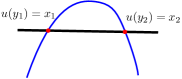
Figure 2. Counting stable maps with tangency

Using the results of [2], all intersection numbers involving the second term on the right hand side of Figure 2 can be computed. Hence, we can compute the characteristic number of rational curves tangent to a given line. Section 9 and Section 10.4 contain a detailed computation along the above line.

We have actually pursued this idea further and computed the characteristic number of rational curves with second order tangency. However, the analysis of the degenerate locus is more intricate.

Finally, in Section 9.3 we pursue this idea again by making the points in the domain come together. This is implemented by extending the idea behind the derivation of Kontsevich’s recursion formula. We choose a suitable subspace of the four pointed moduli space $\overline{M}_{0,4}(\mathbb{CP}^{2},\,d)$ and intersect it with the pullback of two divisors from $\overline{M}_{0,4}$. Equating those two intersection numbers, gives a recursive formula for the characteristic number of rational curves tangent to a given line.

4. The collision lemma

Let $\mathcal{D}_{1}$ be the space of lines in $\mathbb{CP}^{2}$; it is the dual projective space $\widecheck{\mathbb{CP}}^{2}$. Define

$$M \,:=\,\mathcal{D}_{1}\times X_{1}\times X_{2},$$ (4.1)

where $X_{i}$ is a copy of $\mathbb{CP}^{2}$ for $i\,=\,1,\,2$. The pullback to $M$ of the hyperplane classes in $X_{1}$, $X_{2}$ and $\mathcal{D}_{1}$ will be denoted by $a_{1}$, $a_{2}$ and $y_{1}$ respectively. Now define the reduced subscheme

$$X\,:=\,\{(H,\,q_{1},\,q_{2})\,\in\,M\,\,\big{|}\,\,q_{1},\,q_{2}\,\in\,H\},$$

where $M$ is defined in (4.1). Let

$$\iota_{X}\,\,:\,\,X\,\,\hookrightarrow\,M$$ (4.2)

be the inclusion map. Finally, define the reduced hypersurface $Y$ in $X$ as

$$Y \,\,:=\,\,\{(H,\,q_{1},\,q_{2})\,\in\,X\,\,\big{|}\,\,q_{1}\,=\,q_{2}\}\,\,\subset\,\,X.$$ (4.3)

Lemma 4.1 (Collision Lemma).

The line bundle ${\mathcal{O}}_{X}(Y)$ on $X$ (see (4.3)) is given by the divisor class of $\iota^{*}_{X}(a_{1}+a_{2}-y_{1})$ (see (4.2)).

Proof.

Let $\Delta\,\subset\,X_{1}\times X_{2}$ be the reduced diagonal. Let $\text{Bl}_{\Delta}(X_{1}\times X_{2})$ denote the blow-up of $X_{1}\times X_{2}$ along $\Delta$. Note that

$$\text{Bl}_{\Delta}(X_{1}\times X_{2})\,=\,X.$$

This identification sends any $(x_{1},\,x_{2})\,\in\,\mathbb{CP}^{2}_{1}\times\mathbb{CP}^{2}_{2}\setminus\,\Delta$ to $(H,\,x_{1},\,x_{2})\,\in\,X$, where $H$ is the line joining $x_{1}$ and $x_{2}$. The divisor $Y\,\subset\,X$ coincides with the exceptional divisor

$$E\,\subset\,\text{Bl}_{\Delta}(X_{1}\times X_{2}).$$ (4.4)

Let $Z\,:=\,\{(H,\,x)\,\in\,\mathcal{D}_{1}\times\mathbb{CP}^{2}\,\big{|}\,\,x\,\in\,H\}\,\subset\,\mathcal{D}_{1}\times\mathbb{CP}^{2}$ be the reduced divisor. Note that

$$X\,\,=\,\,Z\times_{\mathcal{D}_{1}}Z.$$ (4.5)

This identification sends any $((H,\,x_{1}),\,(H,\,x_{2}))\,\in\,Z\times_{\mathcal{D}_{1}}Z$ to $(H,\,x_{1},\,x_{2})\,\in\,X$. Using this identification, the natural projection

$$\phi\,:\,Z\times_{\mathcal{D}_{1}}Z\,\longrightarrow\,\mathcal{D}_{1}$$ (4.6)

coincides with the restriction to $X$ of the natural projection of $M$ to $\mathcal{D}_{1}$ (see (4.1)). Also, the divisor $Y\,\subset\,X$ coincides with the diagonal divisor

$$\iota_{Z}\,\,:\,\,Z\,\,\hookrightarrow\,\,Z\times_{\mathcal{D}_{1}}Z.$$ (4.7)

For $i\,=\,1,\,2$, consider the following composition of maps

$$Z\times_{\mathcal{D}_{1}}Z\,\stackrel{{\scriptstyle\psi_{i}}}{{\longrightarrow}}\,Z\,\hookrightarrow\,\mathcal{D}_{1}\times\mathbb{CP}^{2}\,\longrightarrow\,\mathbb{CP}^{2},$$

where $\psi_{i}$ is the natural projection to the $i$-th factor and $\mathcal{D}_{1}\times\mathbb{CP}^{2}\,\longrightarrow\,\mathbb{CP}^{2}$ is the projection map. Let $\widetilde{a}_{i}$ be the divisor class on $Z\times_{\mathcal{D}_{1}}Z$ obtained by pulling back the hyperplane class on $\mathbb{CP}^{2}$ using the above composition of maps. Note that the identification in (4.5) takes $\iota^{*}_{X}a_{i}$ to $\widetilde{a}_{i}$, where $\iota_{X}$ is the map in (4.2).

We will show that

$$\phi^{*}{\mathcal{H}}_{1}\,=\,\widetilde{a}_{1}+\widetilde{a}_{2}-\iota_{Z}(Z)$$ (4.8)

(see (4.7) and (4.6)), where ${\mathcal{H}}_{1}$ is the hyperplane class on $\mathcal{D}_{1}$.

Fix a point $(H_{0},\,x_{0})\,\in\,Z$. Consider

$$S_{1}\,:=\,\{((H_{0},\,x),\,(H_{0},\,x_{0}))\,\in\,Z\times_{\mathcal{D}_{1}}Z\,\big{|}\,\,x\,\in\,H_{0}\}\,\subset\,Z\times_{\mathcal{D}_{1}}Z;$$

so $S_{1}$ is identified with the line $H_{0}\,\subset\,\mathbb{CP}^{2}$. The restrictions of the divisor classes $a_{1}$ and $\iota_{Z}(Z)$ to $S_{1}$ are of degree one. The restrictions of the divisor classes $a_{2}$ and $\phi^{*}{\mathcal{H}}_{1}$ to $S_{1}$ are of degree zero. So the restriction of (4.8) to $S_{1}$ is valid. Next consider

$$S_{2}\,:=\,\{((H_{0},\,x_{0}),\,(H_{0},\,x))\,\in\,Z\times_{\mathcal{D}_{1}}Z\,\big{|}\,\,x\,\in\,H_{0}\}\,\subset\,Z\times_{\mathcal{D}_{1}}Z;$$

so $S_{2}$ is identified with the line $H_{0}\,\subset\,\mathbb{CP}^{2}$. The restrictions of the divisor classes $a_{2}$ and $\iota_{Z}(Z)$ to $S_{2}$ are of degree one. The restrictions of the divisor classes $a_{1}$ and $\phi^{*}{\mathcal{H}}_{1}$ to $S_{2}$ are of degree zero. So the restriction of (4.8) to $S_{2}$ is valid.

Consider the line in $\mathcal{D}_{1}$

$${\mathbb{L}}_{x_{0}}\,:=\,\{H\,\in\,\mathcal{D}_{1}\,\,\big{|}\,\,x_{0}\,\in\,H\}\,\subset\,\mathcal{D}_{1},$$

and define

$$S\,:=\,\{((H,\,x_{0}),\,(H,\,x_{0}))\,\in\,Z\times_{\mathcal{D}_{1}}Z\,\big{|}\,\,H\,\in\,{\mathbb{L}}_{x_{0}}\,\subset\,Z\times_{\mathcal{D}_{1}}Z;$$

so $S$ is identified with line ${\mathbb{L}}_{x_{0}}$. The restrictions of the divisor classes $a_{1}$ and $a_{2}$ to $S$ are of degree zero. The restrictions of the divisor classes $\phi^{*}{\mathcal{H}}_{1}$ (respectively, $\iota_{Z}(Z)$) to $S_{2}$ is of degree $1$ (respectively, $-1$). So the restriction of (4.8) to $S$ is valid. Since the restrictions of (4.8) to $S_{1}$, $S_{2}$ and $S$ are valid, we conclude that (4.8) holds.

Since the divisor $Y\,\subset\,X$ coincides with the divisor $\iota_{Z}(Z)\,\subset\,Z\times_{\mathcal{D}_{1}}Z$ by the identification in (4.5), the lemma follows from (4.8). ∎

Define the following divisor class on $M\,=\,\mathcal{D}_{1}\times X_{1}\times X_{2}$

$$\Delta_{1,2}^{\mathsf{L}} \,:=\,a_{1}+a_{2}-y_{1}.$$ (4.9)

The geometric content of the collision lemma is that the intersection of $X$ with the class $\Delta_{1,2}^{\mathsf{L}}$ is equivalent to the class obtained by making the two points come together in $X$.

5. Counting smooth curves with multiple tangencies

Let $\mathcal{D}_{d}$ denote the projective space of dimension $\delta_{d}\,\,=\,\frac{d(d+3)}{2}$ defined by the curves of degree $d$ on the projective plane. Let $X_{1}$ denote a copy of the projective plane. Define the incidence variety

$$\mathrm{I}_{d}\,:=\,\{(H_{d},\,x_{1})\,\in\,\mathcal{D}_{d}\times X_{1}\,\,\big{|}\,\,x_{1}\,\in\,H_{d}\}.$$ (5.1)

Let $a_{1}$ and $y_{d}$ denote the divisor classes on $\mathcal{D}_{d}\times X_{1}$ obtained by pulling back the hyperplane classes on $X_{1}$ and $\mathcal{D}_{d}$ respectively. Then we have

$$[\mathrm{I}_{d}]\,\,=\,\,y_{d}+da_{1}.$$ (5.2)

Indeed, this follows immediately from the fact that the restrictions of (5.2) to both $\{point\}\times\mathbb{CP}^{2}$ and $\mathcal{D}_{d}\times\{point\}$ are valid.

Next, we will study subspaces of $\mathcal{D}_{1}\times\mathcal{D}_{d}\times X_{1}$. First, define $\mathrm{I}_{\mathsf{L}}$ (respectively, $\mathrm{I}_{\mathcal{C}}$) to be the subspace of $\mathcal{D}_{1}\times\mathcal{D}_{d}\times X_{1}$ consisting of all $(H_{1},\,H_{d},\,x_{1})\,\in\,\mathcal{D}_{1}\times\mathcal{D}_{d}\times X_{1}$ such that $x_{1}\,\in\,H_{1}$ (respectively, $x_{1}\,\in\,H_{d}$). Next, define

$$\mathsf{T}_{0}$$ (5.3)

to be the subspace of $\mathcal{D}_{1}\times\mathcal{D}_{d}\times X_{1}$ consisting of all $(H_{1},\,H_{d},\,x_{1})\,\in\,\mathcal{D}_{1}\times\mathcal{D}_{d}\times X_{1}$ such that $H_{1}$ and $H_{d}$ intersect transversally at $x_{1}$. Note that the closure $\overline{\mathsf{T}}_{0}$ comprises of $(H_{1},\,H_{d},\,x_{1})\,\in\,\mathcal{D}_{1}\times\mathcal{D}_{d}\times X_{1}$ such that $x\,\in\,H_{1}\bigcap H_{d}$.

For making the notation easier to read, we will denote the homology class represented by the closure as $[\mathsf{T}_{0}]$ (as opposed to more cumbersome $[\overline{\mathsf{T}}_{0}]$).

Lemma 5.1.

The class $[\mathsf{T}_{0}]\,\in\,H_{2(\delta_{d}+2)}(\mathcal{D}_{1}\times\mathcal{D}_{d}\times X_{1},\,{\mathbb{R}})$ represented by the cycle $\overline{\mathsf{T}}_{0}\,\subset\,\mathcal{D}_{1}\times\mathcal{D}_{d}\times X_{1}$ (see (3.1), (5.3) and (3.1)) is the following:

$$[\mathsf{T}_{0}]\,\,=\,\,[\mathrm{I}_{\mathsf{L}}]\cdot[\mathrm{I}_{\mathcal{C}}],$$ (5.4)

where $[\mathrm{I}_{\mathsf{L}}]$ and $[\mathrm{I}_{\mathcal{C}}]$ are the homology classes of $\mathrm{I}_{\mathsf{L}}$ and $\mathrm{I}_{\mathcal{C}}$ respectively.

Proof.

Consider the divisor $\mathrm{I}_{1}\,\subset\,\mathcal{D}_{1}\times X_{1}$ in (5.1). Let

$$f\,\,:\,\,\mathrm{I}_{1}\times\mathcal{D}_{d}\,\,\hookrightarrow\,\,\mathcal{D}_{1}\times\mathcal{D}_{d}\times X_{1}$$ (5.5)

be the natural map defined by $((H_{1},\,x_{1}),\,H_{d})\,\longmapsto\,(H_{1},\,H_{d},\,x_{1})$, where $(H_{1},\,x_{1})\,\in\,\mathrm{I}_{1}$ and $H_{d}\,\in\,\mathcal{D}_{d}$. Let

$$p\,:\,\mathcal{D}_{1}\times\mathcal{D}_{d}\times X_{1}\,\longrightarrow\,\mathcal{D}_{d}\times X_{1}$$ (5.6)

be the natural projection. Note that

$$\overline{\mathsf{T}}_{0}\,\subset\,\mathrm{I}_{1}\times\mathcal{D}_{d}$$

(see (5.3)) and $\overline{\mathsf{T}}_{0}$ is a divisor.

To prove the lemma it suffices to show the following:

$$f^{*}p^{*}{\mathcal{O}}_{\mathcal{D}_{d}\times X_{1}}(\mathrm{I}_{d})\,=\,{\mathcal{O}}_{\mathrm{I}_{1}\times\mathcal{D}_{d}}(\overline{\mathsf{T}}_{0}).$$ (5.7)

We will now describe three subvarieties $S_{1}$, $S_{2}$ and $S_{3}$ of $\mathrm{I}_{1}\times\mathcal{D}_{d}$. Fix a point $z_{0}\,\in\,\mathrm{I}_{1}$ and define

$$S_{1}\,:=\,\{z_{0}\}\times\mathcal{D}_{d}\,\subset\,\mathrm{I}_{1}\times\mathcal{D}_{d}.$$ (5.8)

Fix curves $(H_{1},\,H_{d})\,\in\,\mathcal{D}_{1}\times\mathcal{D}_{d}$ in $X_{1}$, and we have

$$S_{2}\,:=\,\{(H_{1},\,H_{d},\,x_{1})\,\in\,\mathcal{D}_{1}\times\mathcal{D}_{d}\times X_{1}\,\,\big{|}\,\,x_{1}\,\in\,H_{1}\}\,\subset\,\mathrm{I}_{1}\times\mathcal{D}_{d}.$$ (5.9)

So $S_{2}$ is identified with the line $H_{1}$. Fix a point $x_{0}\,\in\,X_{1}$ and consider the line

$${\mathbb{L}}_{x_{0}}\,:=\,\{H\,\in\,\mathcal{D}_{1}\,\,\big{|}\,\,x_{0}\,\in\,H\}\,\subset\,\mathcal{D}_{1}.$$

Now fix an element $H_{d}\,\in\,\mathcal{D}_{d}$, and define

$$S_{3}\,:=\,\{(H,\,H_{d},\,x_{0})\,\in\,\mathcal{D}_{1}\times\mathcal{D}_{d}\times X_{1}\,\,\big{|}\,\,H\,\in\,{\mathbb{L}}_{x_{0}}\}\,\subset\,\mathrm{I}_{1}\times\mathcal{D}_{d}.$$ (5.10)

Consequently, $S_{3}$ is identified with the line ${\mathbb{L}}_{x_{0}}$.

Given two line bundles ${\mathcal{L}}_{1}$ and ${\mathcal{L}}_{2}$ on $\mathrm{I}_{1}\times\mathcal{D}_{d}$, to show that ${\mathcal{L}}_{1}\,=\,{\mathcal{L}}_{2}$, it is enough to prove that

$${\mathcal{L}}_{1}\big{|}_{S_{j}}\,=\,{\mathcal{L}}_{2}\big{|}_{S_{j}}$$

for $j\,=\,1,\,2,\,3$ (see (5.8), (5.9), (5.10)).

In view of the above criterion it is now straightforward to prove (5.7) using (5.2). ∎

Note that using (5.2), we can rewrite equation (5.4) as

$$[\mathsf{T}_{0}]\,\,=\,\,(y_{1}+a_{1})\cdot(y_{d}+da_{1}),$$ (5.11)

where $\cdot$ denotes topological intersection.

Generalizing $\mathcal{D}_{1}\times\mathcal{D}_{d}\times X_{1}$, define

$$\mathsf{M}_{n}\,\,:=\,\,\mathcal{D}_{1}\times\mathcal{D}_{d}\times(X_{1}\times\cdots\times X_{n}),$$

where $X_{j}$, $1\,\leq\,j\,\leq\,n$, is a copy of $\mathbb{CP}^{2}$. Given nonnegative inters $k_{1},\,\cdots,\,k_{n}$, define

$$[\mathsf{T}_{k_{1}}\ldots\mathsf{T}_{k_{n}}]\,\in\,H_{2(\delta_{d}+2-\sum_{i=1}^{n}k_{i})}(\mathsf{M}_{n},\,\mathbb{R})$$

(see (3.1)) to be the class represented by the closure, in $\mathsf{M}_{n}$, of the subspace $\mathsf{T}_{k_{1}}\ldots\mathsf{T}_{k_{n}}\,\subset\,\mathsf{M}_{n}$ consisting of all $(H_{1},\,H_{d},\,x_{1},\,\cdots,\,x_{n})$ such that

• The points $x_{1},\,\cdots,\,x_{n}$ are all distinct.

• The points $x_{1},\,\cdots,\,x_{n}$ are smooth points of the curve $H_{d}$.

• The line $H_{1}$ intersects the curve $H_{d}$ at the points $x_{1},\,\cdots,\,x_{n}$ with the order of tangencies being $k_{1},\,\cdots,\,k_{n}$ respectively.

Notice that as per its definition, $\mathsf{T}_{1}$ is not a subset of $\mathsf{T}_{0}$, but a subset of the closure $\overline{\mathsf{T}}_{0}$.

Let

$$\pi\,:\,\mathsf{M}_{n+1}\,\longrightarrow\,\mathsf{M}_{n}$$ (5.12)

be the projection that sends any $(H_{1},\,H_{d},\,x_{1},\,\cdots,\,x_{n},\,x_{n+1})$ to $(H_{1},\,H_{d},\,x_{1},\,\cdots,\,x_{n})$. Let

$$\pi_{n+1}\,:\,\mathsf{M}_{n+1}\,\longrightarrow\,\mathsf{M}_{1}$$ (5.13)

be the projection that sends any $(H_{1},\,H_{d},\,x_{1},\,\cdots,\,x_{n},\,x_{n+1})$ to $(H_{1},\,H_{d},\,x_{n+1})$. For any $1\,\leq\,i\,\leq\,n$, let

$$\Delta_{i,{n+1}}\,\,\subset\,\,\mathsf{M}_{n+1}$$

be the locus of all $(H_{1},\,H_{d},\,x_{1},\,\cdots,\,x_{n},\,x_{n+1})$ such that $x_{i}\,=\,x_{n+1}$.

Theorem 5.2.

Let $n$ be a positive integer and $k_{1},\,k_{2},\,\cdots,\,k_{n}$ nonnegative integers with

$$k\,\,:=\,\,k_{1}+k_{2}+\ldots+k_{n}.$$

Then the following equality of elements of $H_{2(\delta_{d}+2-k)}(\mathsf{M}_{n+1},\,{\mathbb{R}})$ holds:

$$\pi^{\ast}[\mathsf{T}_{k_{1}}\ldots\mathsf{T}_{k_{n}}]\cdot\pi_{n+1}^{\ast}[\mathsf{T}_{0}]\,=\,[\mathsf{T}_{k_{1}}\ldots\mathsf{T}_{k_{n}}\mathsf{T}_{0}]+\sum_{i=1}^{n}(k_{i}+1)~{}\pi^{\ast}[\mathsf{T}_{k_{1}}\ldots\mathsf{T}_{k_{n}}]\cdot[\Delta_{i,{n+1}}]$$ (5.14)

(see (5.12), (5.13)) provided $d\,\geq\,k+n$.

Proof.

We will first show that (5.14) is valid on the set-theoretic level. Consider the first term on the left hand side, namely $\pi^{\ast}[\mathsf{T}_{k_{1}}\ldots\mathsf{T}_{k_{n}}]$. It is represented by the closure of the following space: a line, a curve and $n+1$ distinct points $(x_{1},\,\cdots,\,x_{n+1})$, such that the curve is tangent to the line at the points $(x_{1},\,\cdots,\,x_{n})$ to orders $k_{1},\,\cdots,\,k_{n}$ respectively; the last point $x_{n+1}$ is free (it does not have to lie on either the line or the curve).

Now consider second factor on the left hand side of (5.14), namely $\pi_{n+1}^{\ast}[\mathsf{T}_{0}]$. This is simply represented by the following space: a line, a curve and $n+1$ points $(x_{1},\,\cdots,\,x_{n+1})$, such that the points $(x_{1},\,\cdots,\,x_{n})$ are free, while the last point $x_{n+1}$ lies on the line and the curve.

Consider the set-theoretic intersection of the above two spaces. There are two possibilities. The first possibility is that the point $x_{n+1}$ is distinct from all the other points $(x_{1},\,\cdots,\,x_{n})$. The closure of that space represents the first term on the right hand side of (5.14). But there is another possibility. The point $x_{n+1}$ could be equal to one of the $x_{i}$ (for $i\,\in\,\{1,\,\cdots,\,n\}$). On the level of cycles, this space contributes with a multiplicity of $k_{i}+1$. That precisely gives us the second term on the right hand side of (5.14).

To see that equation (5.14) is valid on the level of cycles, it suffices to show that the relevant intersections are transverse as well as justify the multiplicity of the intersection for the second term on the right hand side of (5.14).

We claim that the open part of each of the cycles is actually a smooth manifold of the expected dimension. The first step is to show that $\mathsf{T}_{0}$ is a smooth manifold. We will prove a stronger statement that the closure $\overline{\mathsf{T}}_{0}$ is a smooth manifold.

Let us switch to affine space. Let $\mathcal{F}_{d}$ be the space of polynomials in two variables of degree at most $d$. This is a vector space of dimension $\frac{d(d+3)}{2}+1$, because an element of $\mathcal{F}_{d}$ can be viewed as

$$f(x,\,y)\,:=\,f_{00}+f_{10}x+f_{01}y+\frac{f_{20}}{2}x^{2}+f_{11}xy+\frac{f_{02}}{2}y^{2}+\ldots+\frac{f_{0d}}{d!}y^{d},$$

and hence $f$ can be identified with $(f_{00},\,f_{10},\,f_{01},\,\cdots,\,f_{0d})$. Let $\mathcal{F}_{d}^{*}$ denote the space of nonzero polynomials of degree $d$.

Let us now fix the $x$–axis as designated line. Define $(\mathsf{T}_{0})_{\textsf{Aff}}$ to be the following subspace of $\mathcal{F}_{d}^{*}\times\mathbb{C}$: it consists of a curve $f$ and a complex number $x$ such that the curve transversely passes through the point $(x,\,0)$. It will be shown that $(\mathsf{T}_{0})_{\textsf{Aff}}$ is a smooth submanifold of $\mathcal{F}_{d}^{*}\times\mathbb{C}$. For that, define the map

$$\varphi\,:\,\mathcal{F}_{d}^{*}\times\mathbb{C}\,\longrightarrow\,\mathbb{C},\ \ \ \,(f,\,x)\,\longmapsto\,f(x,\,0).$$

Note that $\overline{(\mathsf{T}_{0})}_{\textsf{Aff}}\,=\,\varphi^{-1}(0)$. In order to show that $\overline{(\mathsf{T}_{0})}_{\textsf{Aff}}$ is a smooth submanifold of $\mathcal{F}_{d}^{*}\times\mathbb{C}$, it suffices to prove that $0$ is a regular value of $\varphi$. To show that $0$ is a regular value of $\varphi$, assume that $\varphi(f,\,x_{1})\,=\,0$. For computing the differential of $\varphi$ at $(f,\,x_{1})$, consider the following curve

$$\gamma(t)\,\,:=\,\,(f+t\eta,\,x),$$

where $\eta$ is as yet an unspecified polynomial. We need to choose $\eta$ in such a way that

$$\{d\varphi|_{(f,x_{1})}\}(\gamma^{\prime}(0))$$

is non-zero. The above expression is

$$\left\{d\varphi\big{|}_{(f,x_{1})}\right\}(\gamma^{\prime}(0))\,\,=\,\,\,\lim_{t\rightarrow\infty}\frac{(f+t\eta)(x_{1},\,0)-f(x_{1},\,0)}{t}\,\,=\,\,\eta(x_{1},\,0).$$

Hence, we require that $\eta(x_{1},\,0)\,\neq\,0$. Clearly such an $\eta$ exists; for example, simply choose $\eta$ to be the polynomial that is identically $1$. Hence, $0$ is a regular value of $\varphi$. This proves that $(\mathsf{T}_{0})_{\textsf{Aff}}$ is a smooth submanifold of $\mathcal{F}_{d}^{*}\times\mathbb{C}$.

Next it will be shown that $\mathsf{T}_{1}$ is a smooth manifold. For that, let $(\mathsf{T}_{1})_{\textsf{Aff}}\,\subset\,\mathcal{F}_{d}^{*}\times\mathbb{C}\,\subset\,\mathcal{F}_{d}^{*}\times\mathbb{C}^{2}$ be the locus of curves and a marked point $(x_{1},\,0)$ contained in the curve such that the curve is tangent to the $x$-axis at $(x_{1},\,0)$ to first order. To show that $(\mathsf{T}_{1})_{\textsf{Aff}}$ is a smooth submanifold of $\mathcal{F}_{d}^{*}\times\mathbb{C}$, define the map

$$\varphi\,\,:\,\,\overline{(\mathsf{T}_{0})}_{\textsf{Aff}}\,\longrightarrow\,\mathbb{C},\ \ \,(f,\,x_{1})\,\longmapsto\,f_{x}(x_{1},\,0).$$

Note that $\overline{(\mathsf{T}_{1})}_{\textsf{Aff}}\,=\,\varphi^{-1}(0)$. In order to prove that $\overline{(\mathsf{T}_{1})}_{\textsf{Aff}}$ is a smooth submanifold of $\mathcal{F}_{d}^{*}\times\mathbb{C}$, it suffices to show that $0$ is a regular value of $\varphi$. For that take $(f,\,x_{1})$ with $\varphi(f,\,x_{1})\,=\,0$. To compute the differential of $\varphi$ at $(f,\,x_{1})$, consider the following curve

$$\gamma(t)\,\,:=\,\,(f+t\eta,\,x_{1}),$$

where $\eta$ is as yet an unspecified polynomial; it should chosen so that

$$\{d\varphi|_{(f,x_{1})}\}(\gamma^{\prime}(0))$$

is non-zero. Furthermore, we need the curve $\gamma(t)$ to lie in $\overline{(\mathsf{T}_{0})}_{\textsf{Aff}}$ for all $t$, i.e., $\eta(x_{1},\,0)\,=\,0$. The differential is given by

$$\{d\varphi|_{(f,x_{1})}\}(\gamma^{\prime}(0))\,\,=\,\,\lim_{t\rightarrow\infty}\frac{(f+t\eta)_{x}(x_{1},\,0)-f_{x}(x_{1},\,0)}{t}\,\,=\,\,\eta_{x}(x_{1},\,0).$$

Hence, $\eta$ should satisfy the conditions that $\eta(x_{1},\,0)\,=\,0$ and $\eta_{x}(x_{1},\,0)\,\neq\,0$. Such an $\eta$ is given by

$$\eta(x,\,y)\,\,=\,\,(x-x_{1}).$$

In order to show that $\overline{\mathsf{T}}_{k}$ is a smooth manifold, we need to find an $\eta$ such that all the derivatives of $\eta$ with respect to $x$, evaluated at $(x_{1},\,0)$ vanish till order $k-1$ and the $k^{\textnormal{th}}$ derivative is non-zero; example of such an $\eta$:

$$\eta(x,\,y)\,\,=\,\,(x-x_{1})^{k}.$$

Notice that this argument works when $d\,\geq\,k$ (otherwise, the above $\eta$ does not exist).

Let us now see what happens when there are multiple points. To show that $\mathsf{T}_{0}\mathsf{T}_{0}$ is a smooth manifold, switch, again, to affine space and define $(\overline{\mathsf{T}}_{0}\overline{\mathsf{T}}_{0})_{\textsf{Aff}}$ as follows:

$$(\overline{\mathsf{T}}_{0}\overline{\mathsf{T}}_{0})_{\textsf{Aff}}\,\,:=\,\,\{(f,\,x_{1},\,x_{2})\,\in\,\mathcal{F}_{d}^{*}\times\mathbb{C}\times\mathbb{C}\,\,\big{|}\,\,f(x_{1},0)\,=\,0,\,\,f(x_{2},0)\,=\,0,\,\,x_{1}\,\neq\,x_{2}\}.$$

To show that $(\overline{\mathsf{T}}_{0}\overline{\mathsf{T}}_{0})_{\textsf{Aff}}$ is a smooth submanifold of $\mathcal{F}_{d}^{*}\times\mathbb{C}\times\mathbb{C}$, define the map

$$\varphi\,:\,\overline{(\mathsf{T}_{0})}_{\textsf{Aff}}\times\mathbb{C}\,\longrightarrow\,\mathbb{C},\ \ \,(f,\,x_{1},\,x_{2})\,\longmapsto\,f(x_{2},\,0).$$

Note that $(\overline{\mathsf{T}}_{0}\overline{\mathsf{T}}_{0})_{\textsf{Aff}}$ is precisely the locus of $(f,\,x_{1},\,x_{2})\,\in\,\varphi^{-1}(0)$ such that $x_{1}\,\neq\,x_{2}$. In order to show that $(\overline{\mathsf{T}}_{0}\overline{\mathsf{T}}_{0})_{\textsf{Aff}}$ is a smooth submanifold of $\mathcal{F}_{d}^{*}\times\mathbb{C}^{2}$, it suffices to show that whenever $\varphi(f,\,x_{1},\,x_{2})\,=\,0$ and $x_{1}\,\neq\,x_{2}$, the differential of $\varphi$ is surjective (i.e., it is non-zero). To prove this, take $(f,\,x_{1},\,x_{2})$ such that $\varphi(f,\,x_{1},\,x_{2})\,=\,0$. To compute the differential of $\varphi$ at $(f,\,x_{1},\,x_{2})$, consider the curve

$$\gamma(t)\,\,:=\,\,(f+t\eta,x_{1},\,x_{2}),$$

where $\eta$ is as yet an unspecified polynomial. It should be so that

$$\{d\varphi|_{(f,x_{1},x_{2})}\}(\gamma^{\prime}(0))$$

is non-zero. Furthermore, the curve $\gamma(t)$ is required to lie in $\overline{(\mathsf{T}_{0})}_{\textsf{Aff}}\times\mathbb{C}$ for all $t$, meaning $\eta(x_{1},\,0)\,=\,0$. The differential is given by

$$\{d\varphi|_{(f,x_{1},x_{2})}\}(\gamma^{\prime}(0))\,\,=\,\,\lim_{t\longrightarrow\infty}\frac{(f+t\eta)(x_{2},\,0)-f(x_{2},\,0)}{t}\,\,=\,\,\eta(x_{2},\,0).$$

Hence, $\eta$ should satisfy $\eta(x_{1},\,0)\,=\,0$ and $\eta(x_{2},\,0)\,\neq\,0$; example of such an $\eta$:

$$\eta(x,\,y)\,\,=\,\,(x-x_{1}).$$

Notice that the condition $x_{1}\,\neq\,x_{2}$ is crucial.

Let us now show that $\mathsf{T}_{k_{1}}\ldots\mathsf{T}_{k_{n}}$ is a smooth manifold. We will prove a stronger statement, namely that $\overline{\mathsf{T}}_{k_{1}}\ldots\overline{\mathsf{T}}_{k_{n}}$ is a smooth manifold, where $\overline{\mathsf{T}}_{k_{1}}\ldots\overline{\mathsf{T}}_{k_{n}}\,\subset\,\mathsf{M}_{n}$ is defined to be the subspace consisting of all $(H_{1},\,H_{d},\,x_{1},\,\cdots,\,x_{n})$ such that

• The points $x_{1},\,\cdots,\,x_{n}$ are all distinct.

• The triple $(H_{1},\,H_{d},\,x_{i})$ belongs to the closure $\overline{\mathsf{T}}_{k_{i}}$ for all $1\,\leq\,i\,\leq\,n$.

Proceeding similarly, we will need to find a curve $\eta$ such that $\eta$ vanishes respectively up to orders $k_{1},\,k_{2},\,\cdots,\,k_{n-1}$ at the points $(x_{1},\,0),\,\cdots,\,(x_{n-1},\,0)$; furthermore, the curve is required to vanish up to to order $k_{n}-1$ at the point $(x_{n},\,0)$ while the derivative of order $k_{n}$ is nonzero at $(x_{n},\,0)$. Such a curve is given by

$$\eta(x,\,y)\,\,=\,\,(x-x_{1})^{k_{1}}(x-x_{2})^{k_{2}}\ldots(x-x_{n-1})^{k_{n-1}}(x-x_{n})^{k_{n}-1}.$$

Notice that this argument works provided $d\,\geq\,k_{1}+k_{2}+\ldots+k_{n}-1$; also the condition that all the $x_{i}$ are distinct is crucial.

Now the multiplicities of the intersections will be computed. The above transversality shows that the first term in the right hand side of (5.14) occurs with multiplicity one. To justify the intersection multiplicities of the remaining terms, consider the situation of $x_{1}$ coinciding with $x_{n+1}$. For convenience, set $(x_{n+1},\,y_{n+1})$ to be the origin. The situation now is that we have a curve $f$ that is tangent to the $x$-axis to order $k_{1}$. We are now going to study the multiplicity with which the evaluation map vanishes at the origin. Hence, $f$ is such that $f_{00},\,f_{10},\,\cdots,\,f_{k_{1}0}$ all vanish. It is given by

$$f(x,\,y)\,\,=\,\,\frac{f_{k_{1}+1,0}}{(k_{1}+1)!}x^{k_{1}+1}+yx+\mathcal{R}(x,\,y),$$

where $\mathcal{R}(x,\,y)$ is an error (or remainder) term. Now consider the evaluation map

$$\varphi(f,\,x)\,\,:=\,\,f(x,\,0)\,\,=\,\,\frac{f_{k_{1}+1,0}}{(k_{1}+1)!}x^{k_{1}+1}.$$

The order of vanishing of $\varphi$ is clearly $k_{1}+1$, provided $f_{k_{1}+1,0}\,\neq\,0$. But that assumption is valid, since to compute the order of vanishing, we will be intersecting with cycles that correspond to constraints being generic. Hence, the order of vanishing is $k_{1}+1$. This proves (5.14) on the level of cycles. ∎

Theorem 5.3.

Let $n$ be a positive integer and $k_{1},\,k_{2},\,\cdots,\,k_{n}$ nonnegative integers with

$$k\,\,:=\,\,k_{1}+k_{2}+\ldots+k_{n}.$$

Then the following equality of elements of $H_{2(\delta_{d}-k)}(\mathsf{M}_{n+1},\,{\mathbb{R}})$ holds:

$$[\mathsf{T}_{k_{1}}\ldots\mathsf{T}_{k_{n-1}}\mathsf{T}_{k_{n}-1}\mathsf{T}_{0}]\cdot[\Delta_{n,{n+1}}^{\mathsf{L}}] =\pi^{*}[\mathsf{T}_{k_{1}}\ldots\mathsf{T}_{k_{n}}]\cdot[\Delta_{n,n+1}],$$ (5.15)

provided $d\,\geq\,k+n$.

Proof.

First consider the special case of this theorem, where $n\,=\,1$ and $k_{1}\,=\,1$. In this case, (5.15) simplifies to

$$[\mathsf{T}_{0}\mathsf{T}_{0}]\cdot[\Delta^{\mathsf{L}}_{12}] \,\,=\,\,\pi^{*}[\mathsf{T}_{1}]\cdot[\Delta_{12}].$$ (5.16)

To prove (5.16), consider the set-up in the proof of Theorem 5.2, where we switch to affine space. The designated line is the $x$–axis. Let $f_{t}$ be a curve that passes through the origin and also through the point $(t,\,0)$. The expression for $f_{t}$ is of the form

$$f_{t}(x,\,y)\,\,=\,\,\varphi_{t}(x)+y\mathcal{R}_{t}(x,\,y),$$

where $\varphi_{t}(x)\,=\,\Big{(}f_{t_{10}}x+\frac{f_{t_{20}}}{2}x^{2}+\ldots\Big{)}$. Since the curve passes through $(t,\,0)$, it follows that

$$\varphi_{t}(x)\,\,=\,\,\Big{(}\mathcal{K}_{t}(x)\Big{)}x(x-t)$$

for some function $\mathcal{K}_{t}(x)$. Denote $f_{0}$ by $f$. Hence,

$$f(x,\,y)\,\,=\,\,\Big{(}\mathcal{K}_{0}(x)\Big{)}x^{2}+y\mathcal{R}_{0}(x,\,y).$$

It is a simple check to see that $f_{00}$ and $f_{10}$ are both zero. Hence, if two $\mathsf{T}_{0}$ points collide, then we get a point which is at least as degenerate as a $\mathsf{T}_{1}$ point (it could be even more degenerate).

Now a more general statement will be proved. Let us show that if $\mathsf{T}_{k}$ and $\mathsf{T}_{0}$ collide, then we get a $\mathsf{T}_{k+1}$. Put the $\mathsf{T}_{k}$ point at $(0,\,0)$ and the $\mathsf{T}_{0}$ point at $(t,\,0)$. The expression for $f_{t}$ is going to be of the form

$$f_{t}(x,\,y) \,=\,\varphi_{t}(x)+y\mathcal{R}_{t}(x,\,y),\ \ \ \textnormal{where}\ \ \varphi_{t}(x)\,=\,\Big{(}f_{t_{10}}x+\frac{f_{t_{20}}}{2}x^{2}+\frac{f_{t_{30}}}{6}x^{3}+\ldots\Big{)}.$$

Since the curve is tangent of the $x$-axis to order $k$ and it also passes through $(t,\,0)$, it follows that

$$\varphi_{t}(x)\,\,=\,\,\Big{(}\mathcal{K}_{t}(x)\Big{)}x^{k+1}(x-t)$$

for some function $\mathcal{K}_{t}(x)$. To see what happens in the limit as $t$ goes to zero, denote $f_{0}$ by $f$. Hence,

$$f(x,\,y)\,\,=\,\,\Big{(}\mathcal{K}_{0}(x)\Big{)}x^{k+2}+y\mathcal{R}_{0}(x,\,y).$$

It is a simple check that $f_{00},\,f_{10},\,\cdots,\,f_{k+1,0}$ are all zero. Hence, if a $\mathsf{T}_{k}$ and a $\mathsf{T}_{0}$ point collide, then we get a point which is at least as degenerate as a $\mathsf{T}_{k+1}$ point (it could be even more degenerate).

In order to complete the proof on the set-theoretic level, it is needed to show that every $\mathsf{T}_{k+1}$ point can be obtained in this way. To see why this is so, first it will be shown why every $\mathsf{T}_{1}$ point can be obtained as a limit to two $\mathsf{T}_{0}$ points.

Let $f\,\in\,(\mathsf{T}_{1})_{\textnormal{Aff}}$. This means that $f_{00}$ and $f_{10}$ are both equal to zero. Hence, $f$ is given by

$$f(x,\,y)\,\,=\,\,\Big{(}\frac{f_{20}}{2}x^{2}+\frac{f_{30}}{6}x^{3}+\ldots\Big{)}+y\mathcal{R}(x,\,y).$$

It will be shown that there exists a point $(f_{t},\,(t,\,0))$ close to $(f,\,(0,\,0))$, such that $f_{t}$ passes through the origin and $(t,\,0)$. Note that since $f_{t}$ passes through the origin, it will be of the form

$$f_{t}(x,\,y)\,=\,f_{t_{10}}x+\Big{(}\frac{f_{t_{20}}}{2}x^{2}+\frac{f_{t_{30}}}{6}x^{3}+\ldots\Big{)}+y\mathcal{R}_{t}(x,\,y).$$

Furthermore, $f_{t_{10}}$ has to be small (since $f_{t}$ is close to $f$ and $f_{10}$ is zero). Impose the condition that $f_{t}(t,\,0)\,=\,0$. Plugging in $(t,\,0)$ inside $f_{t}$ and using the fact that $t\,\neq\,0$, it follows that

$$f_{t_{10}}\,\,=\,\,-\frac{f_{t_{20}}}{2}t+O(t^{2}).$$

Hence, we have constructed this nearby curve $f_{t}$ and a marked point $(t,\,0)$ different from the origin that lies on the curve and the line.

Finally, it will be shown that every element of $\mathsf{T}_{0}\mathsf{T}_{0}$ close to this curve is of this type. This actually fails if $f_{20}\,\neq\,0$. To see how it fails, note that from the construction it follows that the curve $f_{t}$ is unique. But it is a priori possible that the curve could intersect the line at points other than $(0,\,0)$ and $(t,\,0)$. Of course, the curve does intersect it at many points ($d$ points in fact). However, the goal is to find a point that is close to the origin (namely, something that goes to the origin as $t$ goes to zero). It will be shown that the only such point other than the origin is $(t,\,0)$. Let us try to solve the equation

$$f_{t}(x,\,0)\,\,=\,\,0$$

which implies that

$$\Big{(}-\frac{f_{t_{20}}}{2}t+O(t^{2})\Big{)}x+\Big{(}\frac{f_{t_{20}}}{2}x^{2}+\frac{f_{t_{30}}}{6}x^{3}+\ldots\Big{)}\,\,=\,\,0.$$

We are looking for solutions such that $x\,\neq\,0$, and hence may divide out by $x$ and the above equation can be rewritten as

$$\Big{(}-\frac{f_{t_{20}}}{2}t+O(t^{2})\Big{)}+\Big{(}\frac{f_{t_{20}}}{2}x+\frac{f_{t_{30}}}{6}x^{2}+\ldots\Big{)}\,\,=\,\,0.$$

Since $f_{20}\,\neq\,0$, it follows that $f_{t_{20}}\,\neq\,0$. Using the implicit function theorem, $x$ can be uniquely solved in terms of $t$. Hence, the assertion is proved.

We now need to show that every $\mathsf{T}_{k}$ curve is in the limit of a $\mathsf{T}_{k-1}$ and $\mathsf{T}_{0}$. The proof is similar to the above proof of the special case of $k\,=\,1$.

The general case can now proved in a similar way, when there are multiple points. However, there is a subtle point that needs to be addressed. Consider the following assertion

$$[\mathsf{T}_{2}\mathsf{T}_{0}\mathsf{T}_{0}]\cdot[\Delta^{\mathsf{L}}_{23}] \,\,=\,\,\pi^{*}[\mathsf{T}_{2}\mathsf{T}_{1}]\cdot[\Delta_{23}].$$ (5.17)

The proof is almost the same as the proof of (5.16). However, there is one statement that requires further arguments. Recall that we needed to show that every $\mathsf{T}_{1}$ point can be obtained as a limit of two $\mathsf{T}_{0}$ points. In this case, it is needed to show that every $\mathsf{T}_{2}\mathsf{T}_{1}$ point can be obtained as a limit of $\mathsf{T}_{2}\mathsf{T}_{0}\mathsf{T}_{0}$. To see why this is true, recall what has already been proved. Let $f$ be a curve which is tangent to order one to the $x$–axis at the origin. It was shown that there exists a curve $f_{t}$ and a point $(t,\,0)$ such that $f_{t}$ intersects the line transversally at $(0,\,0)$ and $(t,\,0)$. Furthermore, every nearby curve is of that type.

We now have the additional constraint that $f$ intersects the line at say $(a,\,0)$ tangentially to order $2$. Now $f_{t}$ will not necessarily intersect the line tangentially to order $2$. It will be shown that there exists a curve $g_{t}$ close to $f$ such that $g_{t}$ intersects the line at $a$ tangentially to order $2$ (and also intersects the $x$-axis at $(0,\,0)$ and $(t,\,0)$ transversally). For that the following lemma is needed.

Lemma 5.4.

Let $X,\,Y$ and $Z$ be open subsets of $\mathbb{C}^{m},$  $\mathbb{C}^{n}$ and $\mathbb{C}^{k}$ respectively. Let

$$\varphi\,:\,X\times Y\,\longrightarrow\,Z$$

be a holomorphic function such that whenever $\varphi(x,\,y)\,=\,0$, the differential $d\varphi|_{(x,y)}$ restricted to the tangent space $TX|_{x}$ is surjective. For $(x,\,y)$ such that

$$\varphi(x,\,y)\,=\,\varepsilon,$$

where $\varepsilon$ is sufficiently small, there exists a $x_{\varepsilon}$, close to $x$, such that

$$\varphi(x_{\varepsilon},\,y)\,=\,0.$$

Lemma 5.4 follows from the Implicit Function Theorem.

Lemma 5.4 will be used in our setting. Recall that we have a curve $f_{t}$ and three points $(0,\,0)$, $(t,\,0)$ and $(a,\,0)$. Let $X$ denote the subspace of $\mathcal{F}_{d}^{*}$ comprising of curves passing through the points $(0,\,0)$ and $(t,\,0)$. The fact that $X$ is a smooth submanifold of $\mathcal{F}_{d}^{*}$ follows by arguments similar to those showing $(\mathsf{T}_{0}\mathsf{T}_{0})_{\textsf{Aff}}$ is a smooth submanifold of $\mathcal{F}_{d}^{*}\times\mathbb{C}^{2}$; the tangent vector that was used in showing transversality will work in this case as well, because the tangent vector was living entirely in the $\mathcal{F}_{d}^{*}$ slice.

Consider the function

$$\varphi\,:\,X\times\mathbb{C}\,\longrightarrow\,\mathbb{C}^{3},\ \ \,(f,\,x)\,\longmapsto\,(f(x,0),\,f_{x}(x,0),\,f_{xx}(x,0)).$$

Clearly $f_{t}$ belongs to $X$. Note that $\varphi(f_{t},\,a)$ is small (but not necessarily zero). If $\varphi(f,\,a)\,=\,0$, then the differential $d\varphi|_{(f,a)}$ is surjective when restricted to the tangent space of $X$. This is again similar to how it was shown that $(\mathsf{T}_{0}\mathsf{T}_{0}\mathsf{T}_{2})_{\textsf{Aff}}$ is a smooth manifold; the tangent vector used in showing transversality will work here, because the tangent vector lies completely in the $\mathcal{F}_{d}^{*}$ slice. Hence, by Lemma 5.4, there exists a curve $g_{t}$ close to $f_{t}$ such that $g_{t}$ lies in $X$ (i.e., it passes through $(0,\,0)$ and $(t,\,0)$) and it is tangent to order two at $(a,\,0)$. The remaining cases can be proved similarly. This completes the proof of Theorem 5.3. ∎

Note that (5.14) can be rewritten as

$$[\mathsf{T}_{k_{1}}\mathsf{T}_{k_{2}}\ldots\mathsf{T}_{k_{n}}\mathsf{T}_{0}]\,\,=\,\,\pi^{\ast}[\mathsf{T}_{k_{1}}\mathsf{T}_{k_{2}}\ldots\mathsf{T}_{k_{n}}]\cdot\pi_{n+1}^{\ast}[\mathsf{T}_{0}]-\sum_{i=1}^{n}(1+k_{i})~{}\pi^{\ast}[\mathsf{T}_{k_{1}}\mathsf{T}_{k_{2}}\ldots\mathsf{T}_{k_{n}}]\cdot[\Delta_{i,{n+1}}].$$ (5.18)

Also,

$$[\Delta_{i,{n+1}}]\,\,=\,\,a_{i}^{2}+a_{i}a_{n+1}+a_{n+1}^{2}.$$ (5.19)

Let $\beta$ be a class in $\mathsf{M}_{n+1}$ given by

$$\beta\,\,:=\,\,y_{1}^{r}y_{d}^{s}a_{1}^{\varepsilon_{1}}\ldots a_{n+1}^{\varepsilon_{n+1}}.$$

Using (5.11), (5.18) and (5.19), we can recursively compute

$$[\mathsf{T}_{k_{1}}\mathsf{T}_{k_{2}}\ldots\mathsf{T}_{k_{n}}\mathsf{T}_{0}]\cdot\beta$$ (5.20)

for any $\beta$.

Next, let $\alpha$ be a class in $\mathsf{M}_{n}$, given by

$$\alpha\,\,:=\,\,y_{1}^{r}y_{d}^{s}a_{1}^{\varepsilon_{1}}\ldots a_{n}^{\varepsilon_{n}}.$$

Then (5.15) implies that

$$[\mathsf{T}_{k_{1}}\ldots\mathsf{T}_{k_{n}}]\cdot\alpha\,\,=\,\,[\mathsf{T}_{k_{1}}\ldots\mathsf{T}_{k_{n-1}}\mathsf{T}_{k_{n}-1}\mathsf{T}_{0}]\cdot[\Delta_{n,{n+1}}^{\mathsf{L}}]\cdot\alpha.$$ (5.21)

Using equations (4.9), (5.21) and the fact that all the intersection numbers given by (5.20) are computable,

$$[\mathsf{T}_{k_{1}}\mathsf{T}_{k_{2}}\ldots\mathsf{T}_{k_{n}}]\cdot\alpha,$$ (5.22)

can be computed for any $\alpha$.

Note that (5.21) is an equality of numbers; the left hand side is an intersection number in $\mathsf{M}_{n}$, while the right hand side is an intersection number in $\mathsf{M}_{n+1}$. We are using here the convention that if two classes are not of the complementary dimensions, then their intersection number is formally declared to be zero.

6. Counting one nodal curves with multiple tangencies

We now consider plane curves with singularities.

Definition 6.1.

Let $U$ be an open neighbourhood of the origin in $\mathbb{C}$ and let $f\,:\,(U,\,\mathbf{0})\,\longrightarrow\,(\mathbb{C},\,0)$ be a holomorphic function. A point $q\in f^{-1}(0)$ has an $\mathsf{A}_{k}$-singularity if there exists a coordinate system $(x,\,y):(V,\,\mathbf{0})\,\longrightarrow\,(\mathbb{C}^{2},\,\mathbf{0})$ such that $f^{-1}(0)\bigcap V$ is given by

$$y^{2}+x^{k+1} \,\,=\,\,0.$$

An $\mathsf{A}_{1}$-singularity is also called a node, an $\mathsf{A}_{2}$-singularity is called a cusp while an $\mathsf{A}_{3}$-singularity is also called a tacnode.

Define

$$\mathsf{M}_{n}^{m}\,\,:=\,\,\mathcal{D}_{1}\times\mathcal{D}_{d}\times(X^{1}\times\cdots\times X^{m})\times(X_{1}\times\cdots\times X_{n}),$$

where each copy of $X_{i}$ and $X^{j}$ is $\mathbb{CP}^{2}$; the hyperplane classes will be denoted by $a_{i}$ and $b_{j}$ respectively. Let us now define several homology cycles as follows:

• $[\mathsf{A}_{1}^{\mathsf{F}}\mathsf{T}_{k_{1}}\ldots\mathsf{T}_{k_{n}}]\,\in\,H_{\ast}(\mathsf{M}_{n}^{1},\,\mathbb{R})$, where

  $$\mathsf{A}_{1}^{\mathsf{F}}\mathsf{T}_{k_{1}}\ldots\mathsf{T}_{k_{n}}\,\,\subset\,\,\mathsf{M}_{n}^{1}$$

  is the locus of all $(H_{1},\,H_{d},\,p,\,x_{1},\,\cdots,\,x_{n})$ such that the curve $H_{d}$ has a node at $p$ and it is tangent to $H_{1}$ at $x_{1},\,\cdots,\,x_{n}$ with the order of tangencies being $k_{1},\,\cdots,\,k_{n}$ respectively. Furthermore, the points $p,\,x_{1},\,x_{2},\,\cdots,\,x_{n}$ are all distinct.

• $[\mathsf{P}^{(r)}\mathsf{A}_{1}\mathsf{T}_{k_{1}}\ldots\mathsf{T}_{k_{n}}]\,\in\,H_{\ast}(\mathsf{M}_{n}^{1},\,\mathbb{R})$, where

  $$\mathsf{P}^{(r)}\mathsf{A}_{1}\mathsf{T}_{k_{1}}\ldots\mathsf{T}_{k_{n}}\,\subset\,\mathsf{M}_{n}^{1}$$

  is the locus of all $(H_{1},\,H_{d},\,p,\,x_{1},\,\cdots,\,x_{n})$ such that $H_{d}$ has a node at $p$ and one of the branches of the node is tangent to $H_{1}$ at $p$ with the order of tangency being $r$, and $H_{d}$ is tangent to $H_{1}$ at $x_{1},\,\cdots,\,x_{n}$ with the order of tangencies being $k_{1},\,\cdots,\,k_{n}$ respectively. Furthermore, the points $p,\,x_{1},\,x_{2},\,\cdots,\,x_{n}$ are all distinct.

  Notice that if $r\,=\,0$, then $[\mathsf{P}^{(0)}\mathsf{A}_{1}]\,=\,[\mathsf{A}_{1}^{\mathsf{L}}]$, where $\mathsf{A}_{1}^{\mathsf{L}}\,\subset\,\mathsf{M}_{0}^{1}$ is the locus of all $(H_{1},\,H_{d},\,p)$ such that $H_{d}$ has a node at $p$ and $p\,\in\,H_{1}\bigcap H_{d}$. We will use the following notation

  $$[\mathsf{A}_{1}^{\mathsf{L}}]\,\,:=\,\,[\mathsf{P}^{(0)}\mathsf{A}_{1}].$$

  Note that

  $$[\mathsf{A}_{1}^{\mathsf{L}}] \,\,=\,\,[\mathsf{A}_{1}^{\mathsf{F}}]\cdot(y_{1}+b_{1});$$ (6.1)

  this is because intersecting with $(y_{1}+b_{1})$ corresponds to the point $p$ lying on the line.

Proposition 6.2.

The space $\mathsf{A}_{1}^{\mathsf{F}}$ is a smooth submanifold of $\mathsf{M}^{1}_{0}$ of codimension three.

Proof.

The assertion is proved in [11, pp. 216–217], but for the convenience of the reader, we will include the proof here. In fact, we will prove the stronger statement that the closure $\overline{\mathsf{A}_{1}^{\mathsf{F}}}$ is a smooth submanifold of $\mathsf{M}^{1}_{0}$. As before, we will switch to affine space. Consider the map

$$\varphi\,\,:\,\,\mathcal{F}_{d}^{*}\times\mathbb{C}^{2}\,\,\longrightarrow\,\,\mathbb{C}^{3},\ \ \,(f,\,(x,\,y))\,\longmapsto\,(f(x,\,y),\,f_{x}(x,\,y),\,f_{y}(x,\,y)).$$

It suffices to show that $0$ is a regular value of $\varphi$. Consider the polynomials $\eta_{ij}(x,\,y)$ given by

$$\eta_{00}(x,\,y) \,:=\,1,\qquad\eta_{10}(x,\,y)\,:=\,x,\qquad\textnormal{and}\qquad\eta_{01}(x,\,y)\,:=\,y.$$

Let $\gamma_{ij}(t)$ be the curve given by

$$\gamma_{ij}(t)\,\,:=\,\,(f+t\eta_{ij},\,x).$$

Computing the differential of $d\varphi$ on these curves proves transversality. Note that the differential of $\varphi$ restricted to the tangent space of curves is surjective, i.e., the hypothesis of Lemma 5.4 is satisfied. ∎

Theorem 6.3.

Let $n$ be a positive integer, and let $k_{1},\,k_{2},\,\cdots,\,k_{n}$ be nonnegative integers. Define

$$k\,\,:=\,\,k_{1}+k_{2}+\ldots+k_{n}.$$

Then the following equality of homology classes in $H_{*}(\mathsf{M}_{{n+1}}^{1};\,\mathbb{R})$ holds:

$$\pi^{\ast}[\mathsf{A}_{1}^{\mathsf{F}}\mathsf{T}_{k_{1}}\ldots\mathsf{T}_{k_{n}}]\cdot\pi_{n+1}^{\ast}[\mathsf{T}_{0}]\,\,=\,\,[\mathsf{A}_{1}^{\mathsf{F}}\mathsf{T}_{k_{1}}\ldots\mathsf{T}_{k_{n}}\mathsf{T}_{0}]+\sum_{i=1}^{n}(1+k_{i})~{}\pi^{\ast}[\mathsf{A}_{1}^{\mathsf{F}}\mathsf{T}_{k_{1}}\ldots\mathsf{T}_{k_{n}}]\cdot[\Delta_{i,{n+1}}],$$ (6.2)

provided $d\,\geq\,k+n$.

Proof.

This is simply a straightforward generalization of Theorem 5.2; the proof is identical. ∎

Next, we generalize Theorem 5.3.

Theorem 6.4.

Let $n$ be a positive integer, $k_{1},\,k_{2},\,\cdots,\,k_{n-1}$ nonnegative integers and $k_{n}$ a positive integer. Define

$$k \,:=\,k_{1}+k_{2}+\ldots+k_{n}\qquad\textnormal{and}\qquad\mathsf{m}_{k_{n}}\,:=\,\begin{cases}2&~{}~{}\mbox{if}\qquad k_{n}=1,\\ 1&~{}~{}\mbox{if}\qquad k_{n}\,>\,1.\end{cases}$$

On the $(n+1)$–pointed space $\mathsf{M}_{n}^{1}$, let $\alpha$ and $\beta$ be the following classes

$$\alpha \,:=\,y_{1}^{r}y_{d}^{s}b_{1}^{\nu_{\@slowromancap i@}}a_{1}^{\varepsilon_{1}}\ldots a_{n}^{\varepsilon_{n}}\qquad\textnormal{and}\qquad\beta\,:=\,y_{1}^{r}y_{d}^{s}b_{1}^{\nu_{\@slowromancap i@}+\varepsilon_{n}}a_{1}^{\varepsilon_{1}}\ldots a_{n-1}^{\varepsilon_{n-1}}.$$

Then the following equality of numbers holds

$$[\mathsf{A}_{1}^{\mathsf{F}}\mathsf{T}_{k_{1}}\ldots\mathsf{T}_{k_{n-1}}\mathsf{T}_{k_{n}-1}\mathsf{T}_{0}]\cdot[\Delta_{n,{n+1}}^{\mathsf{L}}]\cdot\alpha \,=\,[\mathsf{A}_{1}^{\mathsf{F}}\mathsf{T}_{k_{1}}\ldots\mathsf{T}_{k_{n}}]\cdot\alpha+$$

$$+\mathsf{m}_{k_{n}}~{}\widetilde{\pi}^{\ast}[\mathsf{P}^{(k_{n}-1)}\mathsf{A}_{1}\mathsf{T}_{k_{1}}\ldots\mathsf{T}_{k_{n-1}}]\cdot\beta,$$ (6.3)

provided $d\,\geq\,k+n+1$.

Proof.

First it will be shown that in the special case where $n\,=\,1$ and $k_{n}\,=\,1$, (6.3) simplifies to

$$[\mathsf{A}_{1}^{\mathsf{F}}\mathsf{T}_{0}\mathsf{T}_{0}]\cdot[\Delta_{12}^{\mathsf{L}}]\cdot\alpha \,\,=\,\,[\mathsf{A}_{1}^{\mathsf{F}}\mathsf{T}_{1}]\cdot\alpha+2[\mathsf{A}_{1}^{\mathsf{L}}]\cdot\beta,$$ (6.4)

where

$$\alpha \,\,:=\,\,y_{1}^{r}y_{d}^{s}b_{1}^{\nu_{1}}a_{1}^{\varepsilon_{1}}\qquad\textnormal{and}\qquad\beta\,\,:=\,\,y_{1}^{r}y_{d}^{s}b_{1}^{\nu_{1}+\varepsilon_{1}}.$$

To prove (6.4) it suffices to show the following equality of homology classes in $H_{*}(\mathsf{M}_{\@slowromancap i@,2},\,{\mathbb{R}})$:

$$[\mathsf{A}_{1}^{\mathsf{F}}\mathsf{T}_{0}\mathsf{T}_{0}]\cdot[\Delta_{12}^{\mathsf{L}}] \,=\,\pi^{*}[\mathsf{A}_{1}^{\mathsf{F}}\mathsf{T}_{1}]\cdot[\Delta_{12}]+2\pi^{*}[\mathsf{A}_{1}^{\mathsf{L}}]\cdot[\Delta_{12}]\cdot[\Delta_{\@slowromancap i@,1}].$$ (6.5)

Note that (6.5) is an equality of cycles while (6.4) is an equality of numbers.

The proof of (6.5) builds upon what was already shown in Theorem 5.3, namely when two $\mathsf{T}_{0}$ points collide the first derivative along the line vanishes. Now there are two possibilities. The first one is that the limiting point is a smooth point of the curve. This corresponds to the locus $\mathsf{A}_{1}^{\mathsf{F}}\mathsf{T}_{1}$. There is another possibility that the limiting point is a singular point of the curve. This corresponds to the locus $\mathsf{A}_{1}^{\mathsf{L}}$. On the set-theoretic level, this argument shows that the left hand side of (6.5) is a subset of its right hand side. To show that the right hand side is a subset of the left hand side, we need to show that every element of $\mathsf{A}_{1}^{\mathsf{F}}\mathsf{T}_{1}$ and $\mathsf{A}_{1}^{\mathsf{L}}$ can be obtained as a limit of elements in $\mathsf{A}_{1}^{\mathsf{F}}\mathsf{T}_{0}\mathsf{T}_{0}$. It was shown in the proof of Theorem 5.3 that every element of $\mathsf{T}_{1}$ arises as a limit of elements in $\mathsf{T}_{0}\mathsf{T}_{0}$. To complete the proof here, it is enough to show that every element of $\mathsf{A}_{1}^{\mathsf{F}}\mathsf{T}_{1}$ can be obtained as a limit of elements in $\mathsf{A}_{1}^{\mathsf{F}}\mathsf{T}_{0}\mathsf{T}_{0}$. The argument for it is the same as how we showed (at the end of the proof of Theorem 5.3) that every element of $\mathsf{T}_{1}\mathsf{T}_{2}$ arises as a limit of elements of $\mathsf{T}_{0}\mathsf{T}_{0}\mathsf{T}_{2}$. The crucial fact is what was used in the proof transversality in Proposition 6.2, namely the differential of $\varphi$ restricted to the tangent space of the space of curves is surjective. Hence, using Lemma 5.4 the desired conclusion is reached.

The new thing we need to do for completing the proof of (6.4) (on the set-theoretic level) is to show that every element of $\mathsf{A}_{1}^{\mathsf{L}}$ can be obtained as a limit of elements in $\mathsf{A}_{1}^{\mathsf{F}}\mathsf{T}_{0}\mathsf{T}_{0}$. To prove this assertion, switch to affine space. Let $f$ belong to $(\mathsf{A}_{1}^{\mathsf{L}})_{\textnormal{Aff}}$. As before, the line is the $x$–axis. For convenience, set the nodal point to be the origin. Hence, the expression for $f$ is given by

$$f(x,\,y) \,=\,\frac{f_{20}}{2}x^{2}+f_{11}xy+\frac{f_{02}}{2}y^{2}+\mathcal{R}(x,\,y),$$

where the remainder term $\mathcal{R}(x,\,y)$ is of degree three or higher.

Let us now try to construct a curve $f_{t}$ close to $f$, such that $f_{t}$ passes through the origin, passes through $(t,\,0)$ and has a nodal point close to $(0,\,0)$. The expression for $f_{t}$ will be given by

$$f_{t}(x,\,y) \,=\,f_{t_{10}}x+f_{t_{01}}y+\frac{f_{t_{20}}}{2}x^{2}+f_{t_{11}}xy+\frac{f_{t_{02}}}{2}y^{2}+\ldots$$

First of all, $f_{t_{10}}$ and $f_{t_{01}}$ are small. It is required that $f_{t}$ has a nodal point close to the origin. Hence, we need to find $(u,\,v)\,\neq\,(0,\,0)$ but small, such that

$$f_{t}(u,\,v) \,=\,0,\qquad f_{t_{x}}(u,v)=0\qquad\textnormal{and}\qquad f_{t_{y}}(u,\,v)\,=\,0.$$ (6.6)

To solve (6.6), using the facts that $f_{t_{x}}(u,\,v)\,=\,0$ and $f_{t_{y}}(u,\,v)\,=\,0$ it is deduced that

$$f_{t_{10}} \,=\,-vf_{t_{11}}-uf_{t_{20}}-\mathcal{R}_{x}(u,\,v)\qquad\textnormal{and}\qquad f_{t_{01}}\,=\,-uf_{t_{11}}-vf_{t_{02}}-\mathcal{R}_{y}(u,\,v).$$ (6.7)

Plugging in these values for $f_{t_{10}}$ and $f_{t_{01}}$ from (6.7), and using the fact that $f_{t}(u,\,v)\,=\,0$, it follows that

$$\frac{f_{t_{20}}}{2}u^{2}+f_{t_{11}}uv+\frac{f_{t_{02}}}{2}v^{2}+\mathcal{R}_{2}(u,v)\,\,=\,\,0,\qquad$$ (6.8)

$$\textnormal{where}\qquad\mathcal{R}_{2}(u,\,v):=-2\mathcal{R}(u,\,v)+2u\mathcal{R}_{x}(u,\,v)+2v\mathcal{R}_{y}(u,\,v).$$

Let us now try to solve $u$ in terms of $v$ using (6.8). Since the curve has a genuine node at the origin, it may be assumed that the Hessian is non-degenerate; in other words, $f_{t_{20}}f_{t_{02}}-f_{t_{11}}^{2}$ is non-zero. Hence, after making a change of coordinates and using the fact that the remainder terms $\mathcal{R}_{2}(u,\,v)$ is of order three, it is deduced that there are two solutions to equation (6.8) given by

$$u \,=\,\left(\frac{-f_{t_{11}}+\sqrt{f_{t_{11}}^{2}-f_{t_{20}}f_{t_{02}}}}{f_{t_{20}}}\right)v+O(v^{2})$$

$$\textnormal{or}\qquad u \,=\,\left(\frac{-f_{t_{11}}-\sqrt{f_{t_{11}}^{2}-f_{t_{20}}f_{t_{02}}}}{f_{t_{20}}}\right)v+O(v^{2}).$$

Here $\sqrt{f_{t_{11}}^{2}-f_{t_{20}}f_{t_{02}}}$ is a specific branch of the square root, which exists because $f_{t_{11}}^{2}-f_{t_{20}}f_{t_{02}}$ is non-zero. Hence, the above solution can be re-written as

$$u \,\,=\,\,Av+O(v^{2}),\qquad\textnormal{where}\qquad A\,:=\,\left(\frac{-f_{t_{11}}\pm\sqrt{f_{t_{11}}^{2}-f_{t_{20}}f_{t_{02}}}}{f_{t_{20}}}\right).$$ (6.9)

Now impose the condition that the curve passes through the point $(t,\,0)$. Using (6.9) and the condition that $f_{t}(t,\,0)\,=\,0$ it follows that

$$t \,\,=\,\,2\Big{(}\frac{f_{t_{11}}+Af_{t_{20}}}{f_{t_{20}}}\Big{)}v+O(v^{2}).$$ (6.10)

Hence, the condition of making the two points equal (namely setting $t$  = 0) has a multiplicity, which is is given by (6.10). For each value of $A$, the multiplicity is one. Since there are two possible values of $A$ (corresponding to the branch of the square-root chosen), the total multiplicity is two. Hence, when we intersect with the cycle $[q_{1}\,=\,q_{2}]$, each branch of $\mathsf{A}_{1}^{\mathsf{L}}$ contributes with a multiplicity of $1$ resulting in a total multiplicity is $2$. This property of multiplicity finally shows that (6.5) is true on the level of cycles.

Let us now prove the next case where $n\,=\,1$ and $k_{n}\,=\,k-1$ with $k\,\geq\,3$; denoting $k-1$ by $k_{n}$ makes certain computations more convenient.

Setting $n\,=\,1$ and $k_{n}\,=\,k-1$, equation (6.3) simplifies to

$$[\mathsf{A}_{1}^{\mathsf{F}}\mathsf{T}_{0}\mathsf{T}_{k-2}]\cdot[\Delta_{12}^{\mathsf{L}}]\cdot\alpha\,\,=\,\,[\mathsf{A}_{1}^{\mathsf{F}}\mathsf{T}_{k-1}]\cdot\alpha+[\mathsf{P}^{(k-2)}\mathsf{A}_{1}]\cdot\beta,$$ (6.11)

where

$$\alpha \,\,:=\,\,y_{1}^{r}y_{d}^{s}b_{1}^{\nu_{1}}a_{1}^{\varepsilon_{1}}\qquad\textnormal{and}\qquad\beta\,\,:=\,\,y_{1}^{r}y_{d}^{s}b_{1}^{\nu_{1}+\varepsilon_{1}}.$$

To prove (6.11), it suffices to show the following equality of homology classes in $H_{*}(\mathsf{M}_{\@slowromancap i@,2},\,{\mathbb{R}})$ holds:

$$\pi^{*}[\mathsf{A}_{1}^{\mathsf{F}}\mathsf{T}_{0}\mathsf{T}_{k-2}]\cdot[\Delta_{12}^{\mathsf{L}}] \,=\,\pi^{*}[\mathsf{A}_{1}^{\mathsf{F}}\mathsf{T}_{k-2}]\cdot[\Delta_{12}]+\pi^{*}[\mathsf{P}^{(k-2)}\mathsf{A}_{1}]\cdot[\Delta_{12}]\cdot[\Delta_{\@slowromancap i@,1}].$$ (6.12)

Note that (6.12) is an equality of cycles which implies (6.11) is an equality of numbers.

Let us now prove (6.12). As before, we build up on what we have proved in Theorem 5.3. The justification for the first term on the right hand side of (6.12) is the same as in the proof of Theorem 5.3 (combined with an application of Lemma 5.4). The new thing needed is to justify the second term. In particular, it is needed to show that every element of $\mathsf{P}^{(k-2)}\mathsf{A}_{1}$ can be obtained as a limit of elements in $\mathsf{A}_{1}^{\mathsf{F}}\mathsf{T}_{0}\mathsf{T}_{k-2}$. To prove this assertion, restrict, as before, to affine space.

Let $f$ be a curve that belongs to $\mathsf{P}^{(k-2)}\mathsf{A}_{1}$; the line is set to be the $x$–axis and the nodal point is set to be the origin. We will try to construct a curve $f_{t}$ that is tangent to the $x$–axis at the origin to order $k-2$ (i.e., it is an element of $\mathsf{T}_{k-2}$). It is given by

$$f_{t}(x,\,y) \,=\,uy+\mathsf{P}x^{k-1}+f_{t_{11}}xy+\frac{f_{t_{02}}}{2}y^{2}+\mathsf{Q}x^{k}+\mathcal{R}(x,\,y),\qquad\textnormal{where}$$

$$\mathcal{R}(x,\,y) \,:=\,x^{k+1}\mathsf{A}(x)+yx^{2}\mathsf{B}(x)+y^{2}\mathsf{C}(x,y)\qquad\textnormal{and}\qquad\mathsf{C}(0,\,0)\,=\,0.$$ (6.13)

Notice that $f_{t_{01}}$ is written as $u$. Assume that $\mathsf{Q}\,\neq\,0$. Next, impose the condition that the curve also passes through $(t,\,0)$. In other words, $f_{t}(t,\,0)\,=\,0$. Using this equation and dividing out by $t$, it follows that

$$\mathsf{P} \,\,=\,\,-\mathsf{Q}t+O(t^{2}).$$

Now impose the condition that the curve has a node at $(x,\,y)$. Hence,

$$f_{t}(x,\,y) \,=\,0,\qquad f_{t_{x}}(x,\,y)\,=\,0\qquad\textnormal{and}\qquad f_{t_{y}}(x,\,y)\,=\,0.$$ (6.14)

We are looking for solutions where $u$, $t$, $x$ and $y$ are small and $(x,\,y)\,\neq\,(0,\,0)$. Using the equation $f_{t_{y}}\,=\,0$, it follows that

$$x \,\,=\,\,-\frac{u}{f_{t_{11}}}-\frac{yf_{t_{02}}}{f_{t_{11}}}+\mathcal{E}_{2}(u,y),$$ (6.15)

where the error term $\mathcal{E}_{2}(u,\,y)$ is of second order in $(u,\,y)$. Next, plug this in the equation $f_{t_{x}}(x,\,y)\,=\,0$ and solve for $y$ in terms of $u$ and $t$. This produces

$$(-1)^{k}y \,\,=\,\,\frac{k\mathsf{Q}}{f_{t_{11}}^{k}}u^{k-1}+\frac{(k-1)\mathsf{Q}}{f_{t_{11}}^{k-1}}u^{k-2}t+\mathcal{E}_{k}(u,\,t),$$ (6.16)

where the error term $\mathcal{E}_{k}(u,\,t)$ is of order $k$ in $(u,\,t)$. Plugging all this in $f_{t}(x,\,y)\,=\,0$ gives an implicit relationship between $u$ and $t$. Notice that the expression for $f_{t}(x,\,y)$ will contain a factor of $u^{3}$.

It will be proved that $u$ cannot be zero. Temporarily assume that $u\,\not=\,0$. Since $u\,\neq\,0$, we can cancel off the factor of $u^{3}$ and get a simplified implicit expression for $u$ and $t$. Now we can directly solve for $u$ in terms of $t$ and conclude that

$$u \,\,=\,\,-f_{t_{11}}t+O(t^{2}).$$ (6.17)

Plugging this back into the expression for $x$, gives

$$x \,\,=\,\,t+O(t^{2}).$$ (6.18)

These solutions are the only solutions. Hence, from the expression for $x$ (namely (6.18)), it follows that the multiplicity of the intersection is one. This proves (6.12) on the level of cycles. The general case of Theorem 6.4 now follows in an identical way. This completes the proof of Theorem 6.4. ∎

Theorem 6.5.

Let $n$, $r$ and $k_{1},\,k_{2},\,\cdots,\,k_{n}$ be nonnegative integers. Define

$$k\,\,:=\,\,k_{1}+k_{2}+\ldots+k_{n}.$$

Then the following equality of homology classes of $\mathsf{M}_{n+1}^{1}$ holds:

$$\pi^{\ast}[\mathsf{P}^{(r)}\mathsf{A}_{1}\mathsf{T}_{k_{1}}\mathsf{T}_{k_{2}}\ldots\mathsf{T}_{k_{n}}]\cdot\pi_{n+1}^{\ast}[\mathsf{T}_{0}] \,=\,[\mathsf{P}^{(r)}\mathsf{A}_{1}\mathsf{T}_{k_{1}}\mathsf{T}_{k_{2}}\ldots\mathsf{T}_{k_{n}}\mathsf{T}_{0}]$$

$$+\sum_{i=1}^{n}(k_{i}+1)~{}\pi^{\ast}[\mathsf{P}^{(r)}\mathsf{A}_{1}\mathsf{T}_{k_{1}}\mathsf{T}_{k_{2}}\ldots\mathsf{T}_{k_{n}}]\cdot[\Delta_{i,{n+1}}]$$

$$+(r+2)~{}\pi^{\ast}[\mathsf{P}^{(r)}\mathsf{A}_{1}\mathsf{T}_{k_{1}}\mathsf{T}_{k_{2}}\ldots\mathsf{T}_{k_{n}}]\cdot[\Delta_{{n+1}}^{1}],$$ (6.19)

provided $d\,\geq\,n+k+r+2$.

Proof.

This is a generalization of Theorem 5.2. The new thing needed is to justify the third term on the right hand side of (6.5). The special case of the theorem where $n\,=\,0$ will be proved first. In this special case (6.5) simplifies to

$$\pi^{*}[\mathsf{P}^{(r)}\mathsf{A}_{1}]\cdot\pi_{1}^{*}[\mathsf{T}_{0}] \,\,=\,\,[\mathsf{P}^{(r)}\mathsf{A}_{1}\mathsf{T}_{0}]+(r+2)\pi^{*}[\mathsf{P}^{(r)}\mathsf{A}_{1}]\cdot[\Delta_{1}^{1}].$$ (6.20)

Note that (6.20) is an equality in $H_{*}(\mathsf{M}_{1}^{1},\,\mathbb{R})$.

To prove (6.20), we will first show that $\mathsf{P}^{(r)}\mathsf{A}_{1}$ and $\mathsf{P}^{(r)}\mathsf{A}_{1}\mathsf{T}_{0}$ are smooth manifolds. As before, this will be proved by showing transversality. Let us switch to affine space. It will be shown that $(\mathsf{P}^{(r)}\mathsf{A}_{1})_{\textsf{Aff}}$ is a smooth submanifold of $\mathcal{F}_{d}^{*}\times\mathbb{C}$. For this, define the map

$$\varphi\,\,:\,\,\mathcal{F}_{d}^{*}\times\mathbb{C}\,\,\longrightarrow\,\,\mathbb{C}^{r+3},$$

$$(f,\,x)\,\longmapsto\,\Big{(}f(x,\,0),\,f_{10}(x,\,0),\,f_{01}(x,\,0),\,f_{20}(x,\,0),\,f_{30}(x,\,y),\,\cdots,\,f_{r+1,0}(x,\,0)\Big{)}.$$

Here $f_{ij}(x,\,y)$ denotes the $(i,\,j)^{\textnormal{th}}$ partial derivative of $f$, evaluated at $(x,\,y)$. Note that $(\mathsf{P}^{(r)}\mathsf{A}_{1})_{\textsf{Aff}}$ is $\varphi^{-1}(0)$.

We claim that zero is a regular value of $\varphi$. To prove that, consider the polynomials $\eta_{ij}(x,y)$ given by

$$\eta_{00}(x,\,y) \,:=\,1,\qquad\eta_{10}(x,\,y)\,:=\,x,\qquad\eta_{01}(x,\,y)\,:=\,y,$$

$$\eta_{20}(x,\,y) \,:=\,x^{2},\qquad\eta_{30}(x,\,y)\,:=\,x^{3},\,\cdots\qquad,\,\eta_{r+1,0}(x,\,y)\,:=\,x^{r+1}.$$

Now consider the $r+3$ different curves $\gamma_{ij}(t)$, given by

$$\gamma_{ij}(t)\,\,:=\,\,(f+t\eta_{ij},\,x).$$

Computing the differential of $d\varphi$ on these curves proves transversality. So zero is a regular value of $\varphi$.

Next, it will be shown that $(\mathsf{P}^{(r)}\mathsf{A}_{1}\mathsf{T}_{0})_{\textsf{Aff}}$ is a smooth manifold. Again, we need to achieve transversality. Proceeding as before, we will need to find a curve $\eta$ which has a node at $(x_{1},\,0)$ and all the derivatives in the $x$–direction till order $r+1$ vanish at $(x_{1},\,0)$. Furthermore, the curve should not pass through $(x_{2},\,0)$. Such a curve exists and is given by

$$\eta(x,\,y) \,\,:=\,\,y^{2}+(x-x_{1})y+(x-x_{1})^{r+2}.$$

This shows that the first term on the right hand side of (6.20) occurs with multiplicity one.

Next, let us justify the multiplicity for the second term on the right hand side of (6.20). On the set-theoretic level, the second term is clear. The non-trivial part is to justify the multiplicity of $(r+2)$. This will be done now.

Consider what happens when the $\mathsf{P}^{(r)}\mathsf{A}_{1}$ point and the $\mathsf{T}_{0}$ point coincide. For convenience, set the $\mathsf{P}^{(r)}\mathsf{A}_{1}$ point to be the origin. The situation now is that we have a nodal curve such that one of the branches of the node is tangent to the $x$–axis to order $r$ (at he origin). Hence, the curve $f$ is such that $f_{00},\,f_{10},\,f_{01},\,f_{20},\,\cdots,\,f_{r+1,0}$ all vanish. The function $f$ is given by

$$f(x,\,y) \,\,=\,\,\frac{f_{r+2,0}}{(r+2)!}x^{r+2}+y\mathcal{R}(x,\,y),$$

where $y\mathcal{R}(x,\,y)$ is a remainder term. Now consider the evaluation map

$$\varphi(f,\,x)\,\,:=\,\,f(x,0)\,\,=\,\frac{f_{r+2,0}}{(r+2)!}x^{r+2}.$$

The order of vanishing of $\varphi$ is clearly $r+2$, provided $f_{r+2,0}\,\neq\,0$. But that assumption is valid, since to compute the order of vanishing, we will be intersecting with cycles that correspond to constraints being generic. Hence, the order of vanishing is $r+2$. This proves (6.20) on the level of cycles.

The general statement of Theorem 6.5 is now similar to how Theorem 5.2 is proved. ∎

Theorem 6.6.

Let $n$ be a positive integer, $k_{1},\,k_{2},\,\cdots,\,k_{n-1}$ nonnegative integers and $k_{n}$ a positive integer. Define

$$k \,\,:=\,\,k_{1}+k_{2}+\ldots+k_{n}.$$

On the $(n+1)$–pointed space $\mathsf{M}_{n}^{1}$, let $\alpha$ be the following class

$$\alpha \,\,:=\,\,y_{1}^{r}y_{d}^{s}b_{1}^{\varepsilon_{1}}a_{1}^{\varepsilon_{1}}\ldots a_{n}^{\varepsilon_{n}}.$$

Then the following equality of numbers holds:

$$[\mathsf{P}^{(r)}\mathsf{A}_{1}\mathsf{T}_{k_{1}}\ldots\mathsf{T}_{k_{n-1}}\mathsf{T}_{k_{n}-1}\mathsf{T}_{0}]\cdot[\Delta_{n,{n+1}}^{\mathsf{L}}]\cdot\alpha \,\,=\,\,[\mathsf{P}^{(r)}\mathsf{A}_{1}\mathsf{T}_{k_{1}}\ldots\mathsf{T}_{k_{n}}]\cdot\alpha,$$ (6.21)

provided $d\,\geq\,r+k+n$.

Proof.

This is a generalization of Theorem 5.3; the proof is the same. ∎

Theorem 6.7.

Let $r$ be a positive integer. On $\mathsf{M}^{1}$, define the following class

$$\alpha \,\,:=\,\,y_{1}^{r}y_{d}^{s}b_{1}^{\varepsilon_{1}}.$$

Then the following equality of numbers hold :

$$[\mathsf{P}^{(r-1)}\mathsf{A}_{1}\mathsf{T}_{0}]\cdot[(\Delta^{1}_{1})^{\mathsf{L}}]\cdot\alpha \,\,=\,\,[\mathsf{P}^{(r)}\mathsf{A}_{1}]\cdot\alpha,$$ (6.22)

provided $d\,\geq\,r+3$.

Proof.

First (6.22) will be proved on the set-theoretic level. We switch to affine space. As before, the line is the $x$–axis. Set the $\mathsf{P}^{(r-1)}\mathsf{A}_{1}$ point to be the origin and the $\mathsf{T}_{0}$ point to be $(t,\,0)$. Let $f_{t}$ be a curve that has a $\mathsf{P}^{(r-1)}\mathsf{A}_{1}$ point at the origin and a $\mathsf{T}_{0}$ point at $(t,\,0)$. The former condition says that the first $r$ derivatives with respect to $x$ vanish at the origin. The fact that the curve also passes through $(t,\,0)$ tells that the $(r+1)^{\textnormal{th}}$ derivative is given by

$$f_{r+1,0}\,\,=\,\,-\Big{(}\frac{f_{r+2,0}}{r+2}\Big{)}t+O(t^{2}).$$

Hence, as $t$ goes to zero, $f_{r+1,0}$ vanishes. Furthermore, the curve has a node at the origin. Hence, in the limit, the curve belongs to $\mathsf{P}^{(r)}\mathsf{A}_{1}$.

To complete the proof on the set-theoretic level, it suffices to show that every element of $\mathsf{P}^{(r)}\mathsf{A}_{1}$ arises as a limit of elements of $\mathsf{P}^{(r-1)}\mathsf{A}_{1}\mathsf{T}_{0}$. The proof is exactly the same as how we show every element of $\mathsf{T}_{r+1}$ is a limit of elements of $\mathsf{T}_{r}\mathsf{T}_{0}$. The multiplicity of the intersection also follows in the same way. This proves (6.22) on the level of cycles and completes the proof of Theorem 6.7. ∎

Let us finally note a few things for computational purposes. First, the expression for the homology class $[\mathsf{A}_{1}^{\mathsf{F}}]$ (which is an element of $H_{*}(\mathsf{M}^{1},\,\mathbb{R})$) can be computed using the results of [1]. We will give a new way to derive that expression in Section 8. For now, let us assume that the expression for $[\mathsf{A}_{1}^{\mathsf{F}}]$ is known (which in Section 8.1 we will show is given by (8.1)).

It will now be shown that all the characteristic number of curves with one node tangent to a given line at multiple points to any order can be computed. For this, let $\alpha$ be the following class in $H_{*}(\mathsf{M}_{n}^{1},\,\mathbb{R})$

$$\alpha\,\,:=\,\,y_{1}^{r}y_{d}^{s}b_{1}^{\nu_{1}}a_{1}^{\varepsilon_{1}}\ldots a_{n}^{\varepsilon_{n}}.$$

To compute

$$[\mathsf{A}_{1}^{\mathsf{F}}\mathsf{T}_{k_{1}}\ldots\mathsf{T}_{k_{n}}]\cdot\alpha$$ (6.23)

for any $\alpha$, rewrite (6.2) and (6.21) as follows

$$[\mathsf{A}_{1}^{\mathsf{F}}\mathsf{T}_{k_{1}}\ldots\mathsf{T}_{k_{n}}\mathsf{T}_{0}] \,=\,\pi^{\ast}[\mathsf{A}_{1}^{\mathsf{F}}\mathsf{T}_{k_{1}}\ldots\mathsf{T}_{k_{n}}]\cdot\pi_{n+1}^{\ast}[\mathsf{T}_{0}]$$

$$-\sum_{i=1}^{n}(1+k_{i})~{}\pi^{\ast}[\mathsf{A}_{1}^{\mathsf{F}}\mathsf{T}_{k_{1}}\ldots\mathsf{T}_{k_{n}}]\cdot[\Delta_{i,{n+1}}]\qquad\textnormal{and}$$ (6.24)

$$[\mathsf{A}_{1}^{\mathsf{F}}\mathsf{T}_{k_{1}}\ldots\mathsf{T}_{k_{n}}]\cdot\alpha \,=\,[\mathsf{A}_{1}^{\mathsf{F}}\mathsf{T}_{k_{1}}\ldots\mathsf{T}_{k_{n-1}}\mathsf{T}_{k_{n}-1}\mathsf{T}_{0}]\cdot[\Delta_{n,{n+1}}^{\mathsf{L}}]\cdot\alpha$$

$$-\mathsf{m}_{k_{n}}~{}\widetilde{\pi}^{\ast}[\mathsf{P}^{(k_{n}-1)}\mathsf{A}_{1}\mathsf{T}_{k_{1}}\ldots\mathsf{T}_{k_{n-1}}]\cdot\beta.$$ (6.25)

Using (6.24) and (4.9), the first term on the right hand side of (6.25) is a sum of intersection numbers of the type

$$[\mathsf{A}_{1}^{\mathsf{F}}\mathsf{T}_{k_{1}}\ldots\mathsf{T}_{k_{n}-1}]\cdot\mu$$

for some $\mu$. Hence, in order to compute the expression in (6.23), we have reduced the $k_{n}$ to $k_{n}-1$ (if we consider the first term on the right hand side of (6.25)).

Now consider the second term on the right hand side of (6.25). The goal is to compute

$$[\mathsf{P}^{(k_{n}-1)}\mathsf{A}_{1}\mathsf{T}_{k_{1}}\ldots\mathsf{T}_{k_{n-1}}]\cdot\beta.$$ (6.26)

Rewrite (6.5) and (6.21) as

$$[\mathsf{P}^{(r)}\mathsf{A}_{1}\mathsf{T}_{k_{1}}\mathsf{T}_{k_{2}}\ldots\mathsf{T}_{k_{n}}\mathsf{T}_{0}] \,=\,\pi^{\ast}[\mathsf{P}^{(r)}\mathsf{A}_{1}\mathsf{T}_{k_{1}}\mathsf{T}_{k_{2}}\ldots\mathsf{T}_{k_{n}}]\cdot\pi_{n+1}^{\ast}[\mathsf{T}_{0}]$$

$$-(r+2)~{}\pi^{\ast}[\mathsf{P}^{(r)}\mathsf{A}_{1}\mathsf{T}_{k_{1}}\mathsf{T}_{k_{2}}\ldots\mathsf{T}_{k_{n}}]\cdot[\Delta_{\@slowromancap i@,{n+1}}]$$

$$-\sum_{i=1}^{n}(k_{i}+1)~{}\pi^{\ast}[\mathsf{P}^{(r)}\mathsf{A}_{1}\mathsf{T}_{k_{1}}\mathsf{T}_{k_{2}}\ldots\mathsf{T}_{k_{n}}]\cdot[\Delta_{i,{n+1}}],$$ (6.27)

$$[\mathsf{P}^{(r)}\mathsf{A}_{1}\mathsf{T}_{k_{1}}\ldots\mathsf{T}_{k_{n}}]\cdot\alpha \,=\,[\mathsf{P}^{(r)}\mathsf{A}_{1}\mathsf{T}_{k_{1}}\ldots\mathsf{T}_{k_{n-1}}\mathsf{T}_{k_{n}-1}\mathsf{T}_{0}]\cdot[\Delta_{n,{n+1}}^{\mathsf{L}}]\cdot\alpha.$$ (6.28)

Using (6.28) and (6.27), we can recursively reduce the computation of the expression in (6.26) to the computation of

$$[\mathsf{P}^{(r)}\mathsf{A}_{1}]\cdot\mu$$ (6.29)

for a general $\mu$. To compute the expression in (6.29), rewrite (6.22) as

$$[\mathsf{P}^{(r)}\mathsf{A}_{1}]\cdot\alpha \,\,=\,\,[\mathsf{P}^{(r-1)}\mathsf{A}_{1}\mathsf{T}_{0}]\cdot[(\Delta^{1}_{1})^{\mathsf{L}}]\cdot\alpha.$$ (6.30)

Using (6.30) and (6.27), we reduce the computation of the expression in (6.29) to the computation of

$$[\mathsf{P}^{(0)}\mathsf{A}_{1}]\cdot\mu.$$ (6.31)

But recall that $[\mathsf{P}^{(0)}\mathsf{A}_{1}]$ is the same as $[\mathsf{A}_{1}^{\mathsf{L}}]$; this can be computed from (6.1) and (8.1). Hence, in conclusion, all the intersection numbers in (6.23) can be computed.

7. Counting one cuspidal curves with multiple tangencies of first order

We continue with the set up and notation of Section 6. Define some new homology cycles:

• $[\mathsf{A}_{2}^{\mathsf{F}}\mathsf{T}_{k_{1}}\ldots\mathsf{T}_{k_{n}}]\,\in\,H_{\ast}(\mathsf{M}_{n}^{1},\,\mathbb{R})$, where $\mathsf{A}_{2}^{\mathsf{F}}\mathsf{T}_{k_{1}}\ldots\mathsf{T}_{k_{n}}\,\subset\,\mathsf{M}_{n}^{1}$ is the locus of all

  $$(H_{1},\,H_{d},\,p,\,x_{1},\,\cdots,\,x_{n})$$

  such that the curve $H_{d}$ has a cusp at $p$ and it is tangent to $H_{1}$ at $x_{1},\,\cdots,\,x_{n}$ with the order of tangencies being $k_{1},\,\cdots,\,k_{n}$ respectively. Furthermore, the points $p,\,x_{1},\,x_{2},\,\cdots,\,x_{n}$ are all distinct.

• $[\mathsf{A}_{2}^{\mathsf{L}}\mathsf{T}_{k_{1}}\ldots\mathsf{T}_{k_{n}}]\,\in\,H_{\ast}(\mathsf{M}_{n}^{1},\,\mathbb{R})$, where $\mathsf{A}_{2}^{\mathsf{L}}\mathsf{T}_{k_{1}}\ldots\mathsf{T}_{k_{n}}\,\subset\,\mathsf{M}_{n}^{1}$ is the locus of all

  $$(H_{1},\,H_{d},\,p,\,x_{1},\,\cdots,\,x_{n})$$

  such that the curve $H_{d}$ has a cusp at $p$ and $p\,\in\,H_{1}\bigcap H_{d}$ and it is tangent to $H_{1}$ at $x_{1},\,\cdots,\,x_{n}$ with the order of tangencies being $k_{1},\,\cdots,\,k_{n}$ respectively. Furthermore, the points $p,\,x_{1},\,x_{2},\,\cdots,\,x_{n}$ are all distinct.

Note that

$$[\mathsf{A}_{2}^{\mathsf{L}}] \,\,=\,\,[\mathsf{A}_{2}^{\mathsf{F}}]\cdot(y_{1}+b_{1});$$ (7.1)

this is because intersecting with $(y_{1}+b_{1})$ corresponds to the point $p$ lying on the line. We now start by proving a basic fact about the space of cuspidal curves (similar to Proposition 6.2).

Proposition 7.1.

The space $\mathsf{A}_{2}^{\mathsf{F}}$ is a smooth codimension four submanifold of $\mathsf{M}^{1}_{0}$, provided $d\,\geq\,2$.

Proof.

Unlike before, we will not prove that the closure $\overline{\mathsf{A}_{2}^{\mathsf{F}}}$ is a smooth submanifold. It is in fact usually the case that taking closure makes the space acquire singularities thereby not making it a submanifold.

Let us now prove that $\mathsf{A}_{2}^{\mathsf{F}}$ is a smooth manifold. As before, we will switch to affine space. Consider the map

$$\varphi\,:\,\mathcal{F}_{d}^{*}\times\mathbb{C}^{2}\,\longrightarrow\,\mathbb{C}^{4},\ \ (f,\,(x,\,y))\,\longmapsto\,(f(x,\,y),\,f_{x}(x,\,y),f_{y}(x,\,y),(f_{xx}f_{yy}-f_{xy}^{2})(x,\,y)).$$

It suffices to show that whenever $(x,\,y)$ is a genuine cuspidal point of $f$, the differential of $\varphi$ is surjective.

To prove that the above differential of $\varphi$ is surjective, assume that $(f,\,(x,\,y))\,\in\,\varphi^{-1}(0)$ and that $(x,\,y)$ is a genuine cuspidal point of $f$. In that case, $f_{xx}(x,\,y)$ and $f_{yy}(x,\,y)$ both can’t be zero, because otherwise, even $f_{11}(x,\,y)$ would be zero, making $(x,\,y)$ a triple point of $f$ (i.e., it is not a genuine cusp). Assume that $f_{20}(x,\,y)\,\neq\,0$.

Consider the polynomials $\eta_{ij}(x,\,y)$ given by

$$\eta_{00}(x,\,y) \,=\,1,\qquad\eta_{10}(x,\,y)\,=\,x,\qquad\eta_{01}(x,\,y)\,=\,y\qquad\textnormal{and}\qquad\eta_{20}(x,\,y)\,=\,x^{2}.$$

We have the $4$ different curves $\gamma_{ij}(t)$ given by

$$\gamma_{ij}(t)\,\,:=\,\,(f+t\eta_{ij},\,x).$$

Computing the differential of $d\varphi$ on these curves proves transversality. Note that the differential of $\varphi$ restricted to the tangent space of curves is surjective, so the hypothesis of Lemma 5.4 is satisfied. ∎

The following result enumerates all one cuspidal curves with tangencies at multiple points but all are of first order.

Theorem 7.2.

Let $n$ be a nonnegative integer. Then the following equality of classes in $H_{*}(\mathsf{M}_{{n+1}}^{1},\,\mathbb{R})$ holds:

$$\pi^{\ast}[\mathsf{A}_{2}^{\mathsf{F}}\underbrace{\mathsf{T}_{1}\mathsf{T}_{1}\ldots\mathsf{T}_{1}}_{n}]\cdot\pi_{n+1}^{\ast}[\mathsf{T}_{0}]\,=\,[\mathsf{A}_{2}^{\mathsf{F}}\underbrace{\mathsf{T}_{1}\mathsf{T}_{1}\ldots\mathsf{T}_{1}}_{n}\mathsf{T}_{0}]+\sum_{i=1}^{n}2~{}\pi^{\ast}[\mathsf{A}_{2}^{\mathsf{F}}\underbrace{\mathsf{T}_{1}\mathsf{T}_{1}\ldots\mathsf{T}_{1}}_{n}]\cdot[\Delta_{i,{n+1}}],$$ (7.2)

provided $d\,\geq\,\textnormal{Max}(n+1,\,2)$.

Proof.

This is simply a generalization of Theorems 5.2 and 6.3; the proof is identical. ∎

Theorem 7.3.

Let $n$ be a nonnegative integer. Then the following equality of classes in $H_{*}(\mathsf{M}_{{n+2}}^{1},\mathbb{R})$ holds:

$$\pi^{\ast}[\mathsf{A}_{2}^{\mathsf{F}}\underbrace{\mathsf{T}_{1}\mathsf{T}_{1}\ldots\mathsf{T}_{1}}_{n}\mathsf{T}_{0}]\cdot\pi_{n+2}^{\ast}[\mathsf{T}_{0}] =[\mathsf{A}_{2}^{\mathsf{F}}\underbrace{\mathsf{T}_{1}\mathsf{T}_{1}\ldots\mathsf{T}_{1}}_{n}\mathsf{T}_{0}\mathsf{T}_{0}]$$

$$+\sum_{i=1}^{n}2~{}\pi^{\ast}[\mathsf{A}_{2}^{\mathsf{F}}\underbrace{\mathsf{T}_{1}\mathsf{T}_{1}\ldots\mathsf{T}_{1}}_{n}\mathsf{T}_{0}]\cdot[\Delta_{i,{n+2}}]$$

$$+\pi^{\ast}[\mathsf{A}_{2}^{\mathsf{F}}\underbrace{\mathsf{T}_{1}\mathsf{T}_{1}\ldots\mathsf{T}_{1}}_{n}\mathsf{T}_{0}]\cdot[\Delta_{{n+1},{n+2}}],$$ (7.3)

provided $d\,\geq\,n+2$.

Proof.

Again, this is simply a generalization of Theorem 5.2 and Theorem 6.3; the proof is identical. ∎

Theorem 7.4.

Let $n$ be a positive integer. On the $(n+1)$ pointed space $\mathsf{M}_{n}^{1}$, let $\alpha$ and $\beta$ be the following classes

$$\alpha \,:=\,y_{1}^{r}y_{d}^{s}b_{1}^{\nu_{1}}a_{1}^{\varepsilon_{1}}\ldots a_{n}^{\varepsilon_{n}}\qquad\textnormal{and}\qquad\beta\,:=\,y_{1}^{r}y_{d}^{s}b_{1}^{\nu_{1}+\varepsilon_{n}}a_{1}^{\varepsilon_{1}}\ldots a_{n-1}^{\varepsilon_{n-1}}.$$

Then

$$[\mathsf{A}_{2}^{\mathsf{F}}\underbrace{\mathsf{T}_{1}\ldots\mathsf{T}_{1}}_{n-1}\mathsf{T}_{0}\mathsf{T}_{0}]\cdot[\Delta_{n,{n+1}}^{\mathsf{L}}]\cdot\alpha \,=\,[\mathsf{A}_{2}^{\mathsf{F}}\underbrace{\mathsf{T}_{1}\ldots\mathsf{T}_{1}}_{n}]\cdot\alpha+3\widetilde{\pi}^{\ast}[\mathsf{A}_{2}^{\mathsf{L}}\underbrace{\mathsf{T}_{1}\ldots\mathsf{T}_{1}}_{n-1}]\cdot\beta,$$ (7.4)

provided $d\,\geq\,2n+1$.

Proof.

This is a generalization of Theorem 5.3 and Theorem 6.4. First consider the special case where $n\,=\,1$. Then (7.4) simplifies to

$$[\mathsf{A}_{2}^{\mathsf{F}}\mathsf{T}_{0}\mathsf{T}_{0}]\cdot[\Delta_{12}^{\mathsf{L}}]\cdot\alpha \,\,=\,\,[\mathsf{A}_{2}^{\mathsf{F}}\mathsf{T}_{1}]\cdot\alpha+3[\mathsf{A}_{2}^{\mathsf{L}}]\cdot\beta,$$ (7.5)

where

$$\alpha \,=\,y_{1}^{r}y_{d}^{s}b_{1}^{\nu_{1}}a_{1}^{\varepsilon_{1}}\qquad\textnormal{and}\qquad\beta\,=\,y_{1}^{r}y_{d}^{s}b_{1}^{\nu_{1}+\varepsilon_{1}}.$$

To prove (7.5) it suffices to show the following equality of homology classes in $H_{*}(\mathsf{M}_{2}^{1},\,{\mathbb{R}})$:

$$[\mathsf{A}_{2}^{\mathsf{F}}\mathsf{T}_{0}\mathsf{T}_{0}]\cdot[\Delta_{12}^{\mathsf{L}}] \,\,=\,\,\pi^{*}[\mathsf{A}_{2}^{\mathsf{F}}\mathsf{T}_{1}]\cdot[\Delta_{12}]+3\pi^{*}[\mathsf{A}_{2}^{\mathsf{L}}]\cdot[\Delta_{12}]\cdot[\Delta_{1}^{1}].$$ (7.6)

Note that (7.5) is an equality of cycles while (7.6) is an equality of numbers.

To prove (7.6), the first term on the right hand side of (7.6) is explained the same way the first term on the right hand side of (6.5) is explained. The new thing is to interpret the second term. Let us first explain this term at the set-theoretic level.

It was already shown that when two $\mathsf{T}_{0}$ points collide, the first derivative along the line vanishes. When the resulting point is smooth, the locus $\mathsf{A}_{2}^{\mathsf{F}}\mathsf{T}_{1}$ is obtained. When the resulting point is not smooth, the locus $\mathsf{A}_{2}^{\mathsf{L}}$ is obtained. To complete the proof on the set-theoretic level, we need to show that every point of $\mathsf{A}_{2}^{\mathsf{F}}\mathsf{T}_{1}$ and $\mathsf{A}_{2}^{\mathsf{L}}$ arises this way. The first assertion is proved exactly as before using Lemma 5.4 and Proposition 7.1.

Let us now show that every point of $\mathsf{A}_{2}^{\mathsf{L}}$ arises as a limit of $\mathsf{A}_{2}^{\mathsf{F}}\mathsf{T}_{0}\mathsf{T}_{0}$. As before, we will be working in affine space. Take $f\,\in\,(\mathsf{A}_{2}^{\mathsf{L}})_{\textsf{Aff}}$. As usual, the line is the $x$–axis and the cuspidal point is the origin. Assume that $f_{20}\,\neq\,0$; here $f_{ij}$ denotes the $(i,\,j)^{\textnormal{th}}$ derivative at the origin. Let $f_{t}$ be a curve close to $f$ that passes through the origin and also passes through $(t,\,0)$. The Taylor expansion of $f_{t}$ is

$$f_{t}(x,\,y)\,=\,uy+\mathsf{P}x+\frac{f_{t_{20}}}{2}x^{2}+f_{t_{11}}xy+\frac{1}{2}\Big{(}s+\frac{f_{t_{11}}^{2}}{f_{t_{20}}}\Big{)}y^{2}+\frac{f_{t_{30}}}{6}x^{3}+$$

$$\frac{f_{t_{21}}}{2}x^{2}y+\frac{f_{t_{12}}}{2}xy^{2}+\frac{f_{t_{03}}}{6}y^{3}+\mathcal{E}_{4}(x,\,y),$$

where the error term $\mathcal{E}_{4}(x,\,y)$ is fourth order in $(x,\,y)$. Here $f_{t_{01}}$ is denoted by $u$ and $f_{t_{10}}$ is denoted by $\mathsf{P}$.

Now impose the condition that the curve passes through $(t,\,0)$, so $f_{t}(t,\,0)\,=\,0$. This implies that

$$\mathsf{P} \,\,=\,\,-\frac{f_{t_{20}}}{2}t+O(t^{2}).$$ (7.7)

Now impose the condition that the curve has a cuspidal point at $(x,\,y)$. This implies that

$$f_{t}(x,\,y) \,=\,0,\qquad f_{t_{x}}(x,\,y)\,=\,0,\qquad f_{t_{y}}(x,\,y)\,=\,0\qquad\textnormal{and}\qquad H_{f_{t}}\,:=\,f_{t_{xx}}f_{t_{yy}}-f_{t_{xy}}^{2}\,=\,0.$$ (7.8)

Using the conditions that $f_{t_{x}}\,=\,0$ and $f_{t_{y}}\,=\,0$ it follows that

$$\frac{f_{t_{20}}}{2}t \,=\,yf_{t_{11}}+xf_{t_{20}}+\frac{f_{t_{12}}}{2}y^{2}+f_{t_{21}}xy+\frac{f_{t_{30}}}{2}x^{2}+\mathcal{E}_{3}(x,\,y)\qquad\textnormal{and}$$ (7.9)

$$-u \,=\,\Big{(}s+\frac{f_{t_{11}}^{2}}{f_{t_{20}}}\Big{)}y+xf_{t_{11}}+\frac{f_{t_{03}}}{2}y^{2}+f_{t_{12}}xy+\frac{f_{t_{21}}}{2}x^{2}+\widetilde{\mathcal{E}}_{3}(x,\,y).$$ (7.10)

Next, use the condition $H_{f_{t}}\,=\,0$ to conclude that

$$-s \,=\,\Big{(}f_{t_{12}}+\frac{f_{t_{11}}^{2}f_{t_{30}}}{f_{t_{20}}^{2}}\Big{)}x+\Big{(}f_{t_{30}}-\frac{2f_{t_{11}}f_{t_{12}}}{f_{t_{20}}}+\frac{f_{t_{11}}^{2}f_{t_{21}}}{f_{t_{20}}^{2}}\Big{)}y.$$ (7.11)

Finally, plugging all these in $f_{t}(x,\,y)\,=\,0$, it follows that

$$-\frac{(f_{t_{20}}x+f_{t_{11}}y)^{2}}{2f_{t_{20}}}- \frac{f_{t_{30}}}{3}x^{3}-f_{t_{21}}x^{2}y+xy^{2}\Big{(}\frac{f_{t_{11}}^{2}f_{t_{30}}}{2f_{t_{20}}^{2}}-\frac{f_{t_{12}}}{2}\Big{)}$$

$$+ \Big{(}\frac{f_{t_{03}}}{6}-\frac{f_{t_{11}}f_{t_{12}}}{f_{t_{20}}}+\frac{f_{t_{11}}^{2}f_{t_{21}}}{2f_{t_{20}}^{2}}\Big{)}y^{3}\,=\,0.$$ (7.12)

Next, make the following change of coordinates

$$\widehat{x} \,\,:=\,\,f_{t_{20}}x+f_{t_{11}}y\qquad\textnormal{and}\qquad\widehat{y}\,\,:=\,\,y.$$ (7.13)

Note that this is a valid change of coordinate because $f_{t_{20}}\,\not=\,0$. Under a further genericity assumption on the third derivatives, we can make a change of coordinates (centred around the origin) so that (7.12) can be rewritten as

$$\widehat{x}^{2}-\widehat{y}^{3} \,\,=\,\,0.$$ (7.14)

Equation (7.14) has exactly one solution close to the origin, namely

$$\widehat{x} \,\,=\,\,v^{3}\qquad\textnormal{and}\qquad\widehat{y}\,\,=\,\,v^{2}.$$ (7.15)

Using (7.9), (7.13) and (7.15) it follows that

$$t \,\,=\,\,\frac{2}{f_{t_{20}}}v^{3}+O(v^{4}).$$ (7.16)

Since we are setting $t$ to be equal to zero to obtain the $\mathsf{A}_{2}^{\mathsf{L}}$ point, (7.16) implies that the multiplicity of the intersection in the second term on the right hand side of (7.6) is $3$. This proves (7.6). Note that the assumption $f_{t_{20}}\,\not=\,0$ and the genericity assumption of the third derivative is valid, since to compute the multiplicity of intersections, we will intersect with a generic cycle. The general case now follows as before. ∎

Theorem 7.5.

Let $n$ be a nonnegative integer. Let $\alpha$ and $\beta$ be the following classes in $H_{*}(\mathsf{M}_{n+2}^{1},\,\mathbb{R})$:

$$\alpha \,:=\,y_{1}^{r}y_{d}^{s}b_{1}^{\nu_{1}}a_{1}^{\varepsilon_{1}}\ldots a_{n+2}^{\varepsilon_{n+2}}\qquad\textnormal{and}\qquad\beta\,:=\,y_{1}^{r}y_{d}^{s}b_{1}^{\nu_{1}}a_{1}^{\varepsilon_{1}}\ldots a_{n+1}^{\varepsilon_{n+1}+\varepsilon_{n+2}}.$$

Then

$$[\mathsf{A}_{2}^{\mathsf{L}}\underbrace{\mathsf{T}_{1}\ldots\mathsf{T}_{1}}_{n}\mathsf{T}_{0}\mathsf{T}_{0}]\cdot[\Delta_{{n+1},{n+2}}^{\mathsf{L}}]\cdot\alpha \,\,=\,\,[\mathsf{A}_{2}^{\mathsf{L}}\underbrace{\mathsf{T}_{1}\ldots\mathsf{T}_{1}}_{n+1}]\cdot\beta,$$ (7.17)

provided $d\,\geq\,2n+2$.

Proof.

This is a generalization of Theorem 5.3 and Theorem 6.6; the proof is the same. ∎

Theorem 7.6.

Let $n$ be a nonnegative integer. Then the following equality of classes in $H_{*}(\mathsf{M}_{{n+1}}^{1},\,\mathbb{R})$ holds:

$$\pi^{\ast}[\mathsf{A}_{2}^{\mathsf{L}}\underbrace{\mathsf{T}_{1}\mathsf{T}_{1}\ldots\mathsf{T}_{1}}_{n}]\cdot\pi_{n+1}^{\ast}[\mathsf{T}_{0}] \,=\,[\mathsf{A}_{2}^{\mathsf{L}}\underbrace{\mathsf{T}_{1}\mathsf{T}_{1}\ldots\mathsf{T}_{1}}_{n}\mathsf{T}_{0}]+\sum_{i=1}^{n}2~{}\pi^{\ast}[\mathsf{A}_{2}^{\mathsf{L}}\underbrace{\mathsf{T}_{1}\mathsf{T}_{1}\ldots\mathsf{T}_{1}}_{n}]\cdot[\Delta_{i,{n+1}}]$$

$$+2~{}\pi^{\ast}[\mathsf{A}_{2}^{\mathsf{L}}\underbrace{\mathsf{T}_{1}\mathsf{T}_{1}\ldots\mathsf{T}_{1}}_{n}]\cdot[\Delta_{{n+1}}^{1}],$$ (7.18)

provided $d\,\geq\,n+3$.

Proof.

This is a generalization of Theorem 6.5. The new thing we need to show is to justify the third term on the right hand side of (7.6).

Let us first prove the special case of Theorem 7.6 where $n\,=\,0$. In this case (7.6) simplifies to

$$\pi^{*}[\mathsf{A}_{2}^{\mathsf{L}}]\cdot\pi_{1}^{*}[\mathsf{T}_{0}] \,\,=\,\,[\mathsf{A}_{2}^{\mathsf{L}}\mathsf{T}_{0}]+2\pi^{*}[\mathsf{A}_{2}^{\mathsf{L}}]\cdot[\Delta_{1}^{1}].$$ (7.19)

The first step to prove (7.19) would be to show that $\mathsf{A}_{2}^{\mathsf{L}}$ and $\mathsf{A}_{2}^{\mathsf{L}}\mathsf{T}_{0}$ are smooth manifolds. As before, this will be proved by showing transversality. Let us switch to affine space.

To show that $(\mathsf{A}_{2}^{\mathsf{F}})_{\textsf{Aff}}$ is a smooth submanifold of $\mathcal{F}_{d}^{*}\times\mathbb{C}$, define the map

$$\varphi\,:\,\mathcal{F}_{d}^{*}\times\mathbb{C} \,\longrightarrow\,\mathbb{C}^{4},$$

$$(f,\,x) \,\longmapsto\,\Big{(}f(x,\,0),~{}f_{10}(x,\,0),~{}f_{01}(x,\,0),~{}(f_{20}f_{02}-f_{11}^{2})(x,\,0)\Big{)}.$$

Here $f_{ij}(x,\,y)$ denotes the $(i,\,j)^{\textnormal{th}}$ partial derivative of $f$, evaluated at $(x,\,y)$. Note that $(\mathsf{A}_{2}^{\mathsf{L}})_{\textsf{Aff}}$ is an open dense subset of $\varphi^{-1}(0)$ (the latter contains points that are more degenerate than an $\mathsf{A}_{2}$ singularity). We will show that the differential $d\varphi_{(f,x)}$ is surjective, whenever $(x,\,0)$ is a genuine cuspidal point of $f$.

Suppose that $\varphi(f,\,x)\,=\,0$ and $(x,\,0)$ is a genuine cuspidal point of $f$. This means that $f_{20}(x,0)$ and $f_{02}(x,0)$ both can’t be zero, because otherwise $f_{11}$ would also be zero and the singularity would be a triple point (which is more degenerate than a cusp). Assume $f_{20}(x,\,0)\,\not=\,0$. Consider the polynomials $\eta_{ij}(x,y)$ given by

$$\eta_{00}(x,\,y) \,:=\,1,\qquad\eta_{10}(x,\,y)\,:=\,x,\qquad\eta_{01}(x,\,y)\,:=\,y\qquad\textnormal{and}\qquad\eta_{20}(x,\,y)\,:=\,x^{2}.$$

Let $\gamma_{ij}(t)$ be the $4$ different curves defined by

$$\gamma_{ij}(t)\,\,:=\,\,(f+t\eta_{ij},x).$$

Computing the differential of $d\varphi$ on these curves proves transversality.

Next, it will be shown that $(\mathsf{A}_{2}^{\mathsf{L}}\mathsf{T}_{0})_{\textsf{Aff}}$ is a smooth manifold; this will be done using transversality. Proceeding as before, we will need to find a curve $\eta$, such that it has a cuspidal point at $(x_{1},\,0)$ and the curve should not pass through $(x_{2},\,0)$. Such a curve exists and is given by

$$\eta(x,\,y) \,\,:=\,\,(x-x_{1})^{2}+y^{3}.$$

This shows that the first term on the right hand side of (7.19) occurs with a multiplicity of one.

Next, let us justify the multiplicity for the second term on the right hand side of (7.19). On the set-theoretic level, the second term is clear. The nontrivial part is to justify the multiplicity $2$.

Consider what happens when the $\mathsf{A}_{2}^{\mathsf{L}}$ point and the $\mathsf{T}_{0}$ point coincide. For convenience, set the $\mathsf{A}_{2}^{\mathsf{L}}$ point to be the origin. We are now going to study the multiplicity with which the evaluation map vanishes at the origin. Note that the curve $f$ is such that $f_{00}$,  $f_{10}$,  $f_{01}$,  $f_{20}f_{02}-f_{11}^{2}$ all vanish. Further assume that $f_{20}\,\neq\,0$. Consequently, the curve is given by

$$f(x,\,y) \,=\,\frac{f_{20}}{2}x^{2}+f_{11}xy+\frac{f_{11}^{2}}{f_{02}}y^{2}+\mathcal{R}(x,\,y),$$

where $\mathcal{R}(x,\,y)$ is a remainder term of order three. The order of vanishing of the evaluation map should be $2$. To see why that is so, consider the evaluation map

$$\varphi(f,\,x) \,:=\,f(x,\,0)\,=\,\frac{f_{20}}{2}x^{2}+O(x^{3}).$$

Since by assumption $f_{20}\,\neq\,0$, we conclude that the order of vanishing is $2$. The assumption that $f_{20}\,\neq\,0$ is valid, since to compute the multiplicity of intersections, we intersect with generic cycles. This proves (7.19) on the level of cycles. The general statement now follows similarly. ∎

Theorem 7.7.

Let $n$ be a nonnegative integer. Then the following equality of classes in $H_{*}(\mathsf{M}_{{n+1}}^{1},\,\mathbb{R})$ holds:

$$\pi^{\ast}[\mathsf{A}_{2}^{\mathsf{L}}\underbrace{\mathsf{T}_{1}\mathsf{T}_{1}\ldots\mathsf{T}_{1}}_{n}\mathsf{T}_{0}]\cdot\pi_{n+2}^{\ast}[\mathsf{T}_{0}] \,=\,[\mathsf{A}_{2}^{\mathsf{L}}\underbrace{\mathsf{T}_{1}\mathsf{T}_{1}\ldots\mathsf{T}_{1}}_{n}\mathsf{T}_{0}\mathsf{T}_{0}]+2~{}\pi^{\ast}[\mathsf{A}_{2}^{\mathsf{L}}\underbrace{\mathsf{T}_{1}\mathsf{T}_{1}\ldots\mathsf{T}_{1}}_{n}\mathsf{T}_{0}]\cdot[\Delta_{\@slowromancap i@,{n+2}}]$$

$$+\pi^{\ast}[\mathsf{A}_{2}^{\mathsf{L}}\underbrace{\mathsf{T}_{1}\mathsf{T}_{1}\ldots\mathsf{T}_{1}}_{n}\mathsf{T}_{0}]\cdot[\Delta_{n+1,{n+2}}]$$

$$+\sum_{i=1}^{n}2~{}\pi^{\ast}[\mathsf{A}_{2}^{\mathsf{L}}\underbrace{\mathsf{T}_{1}\mathsf{T}_{1}\ldots\mathsf{T}_{1}}_{n}\mathsf{T}_{0}]\cdot[\Delta_{i,{n+2}}],$$ (7.20)

provided $d\,\geq\,n+4$.

Proof.

The proof is the same as that of Theorem 7.6. ∎

Let us finally note a few things for computational purposes. First, the expression for the homology class $[\mathsf{A}_{2}^{\mathsf{F}}]$ (which is an element of $H_{*}(\mathsf{M}^{1},\,\mathbb{R})$) can be computed using the results of [1], given by

$$[\mathsf{A}_{2}^{\mathsf{F}}] =\big{(}12d^{2}-36d+24\big{)}y_{d}^{2}b_{1}^{2}+\big{(}8d-12\big{)}y_{d}^{3}b_{1}+2y_{d}^{4}.$$ (7.21)

It will be shown how the characteristic number of curves with one cusp, tangent to a given line at multiple points to first order can be computed. For this, let $\alpha$ be the following class in $H_{*}(\mathsf{M}_{n}^{1},\mathbb{R})$

$$\alpha \,\,:=\,\,y_{1}^{r}y_{d}^{s}b_{1}^{\nu_{1}}a_{1}^{\varepsilon_{1}}\ldots a_{n}^{\varepsilon_{n}}.$$

In order to compute

$$[\mathsf{A}_{2}^{\mathsf{F}}\underbrace{\mathsf{T}_{1}\ldots\mathsf{T}_{1}}_{n}]\cdot\alpha$$ (7.22)

for any $\alpha$, first of all rewrite (7.4) as

$$[\mathsf{A}_{2}^{\mathsf{F}}\underbrace{\mathsf{T}_{1}\ldots\mathsf{T}_{1}}_{n}]\cdot\alpha \,=\,[\mathsf{A}_{2}^{\mathsf{F}}\underbrace{\mathsf{T}_{1}\ldots\mathsf{T}_{1}}_{n-1}\mathsf{T}_{0}\mathsf{T}_{0}]\cdot[\Delta_{n,{n+1}}^{\mathsf{L}}]\cdot\alpha-\widetilde{\pi}^{\ast}[\mathsf{A}_{2}^{\mathsf{L}}\underbrace{\mathsf{T}_{1}\ldots\mathsf{T}_{1}}_{n-1}]\cdot\beta.$$ (7.23)

Furthermore, rewrite (7.2) and (7.3) as

$$[\mathsf{A}_{2}^{\mathsf{F}}\underbrace{\mathsf{T}_{1}\mathsf{T}_{1}\ldots\mathsf{T}_{1}}_{n}\mathsf{T}_{0}] \,=\,\pi^{\ast}[\mathsf{A}_{2}^{\mathsf{F}}\underbrace{\mathsf{T}_{1}\mathsf{T}_{1}\ldots\mathsf{T}_{1}}_{n}]\cdot\pi_{n+1}^{\ast}[\mathsf{T}_{0}]$$

$$-\sum_{i=1}^{n}2~{}\pi^{\ast}[\mathsf{A}_{2}^{\mathsf{F}}\underbrace{\mathsf{T}_{1}\mathsf{T}_{1}\ldots\mathsf{T}_{1}}_{n}]\cdot[\Delta_{i,{n+1}}]\qquad\textnormal{and}$$ (7.24)

$$[\mathsf{A}_{2}^{\mathsf{F}}\underbrace{\mathsf{T}_{1}\mathsf{T}_{1}\ldots\mathsf{T}_{1}}_{n}\mathsf{T}_{0}\mathsf{T}_{0}] \,=\,\pi^{\ast}[\mathsf{A}_{2}^{\mathsf{F}}\underbrace{\mathsf{T}_{1}\mathsf{T}_{1}\ldots\mathsf{T}_{1}}_{n}\mathsf{T}_{0}]\cdot\pi_{n+2}^{\ast}[\mathsf{T}_{0}]-\sum_{i=1}^{n}2~{}\pi^{\ast}[\mathsf{A}_{2}^{\mathsf{F}}\underbrace{\mathsf{T}_{1}\mathsf{T}_{1}\ldots\mathsf{T}_{1}}_{n}\mathsf{T}_{0}]\cdot[\Delta_{i,{n+2}}]$$

$$-\pi^{\ast}[\mathsf{A}_{2}^{\mathsf{F}}\underbrace{\mathsf{T}_{1}\mathsf{T}_{1}\ldots\mathsf{T}_{1}}_{n}\mathsf{T}_{0}]\cdot[\Delta_{{n+1},{n+2}}].$$ (7.25)

Using (7.25) and (7.24), the computation of the first term on the right hand side of (7.23) reduces to a computation of

$$[\mathsf{A}_{2}^{\mathsf{F}}\underbrace{\mathsf{T}_{1}\ldots\mathsf{T}_{1}}_{n-1}]\cdot\mu$$

for any $\mu$. Using (7.21), this can be recursively computed. Let us now see how to compute the second term on the right hand side of (7.23).

Rewrite (7.6) and (7.7) as

$$[\mathsf{A}_{2}^{\mathsf{L}}\underbrace{\mathsf{T}_{1}\mathsf{T}_{1}\ldots\mathsf{T}_{1}}_{n}\mathsf{T}_{0}] \,=\,\pi^{\ast}[\mathsf{A}_{2}^{\mathsf{L}}\underbrace{\mathsf{T}_{1}\mathsf{T}_{1}\ldots\mathsf{T}_{1}}_{n}]\cdot\pi_{n+1}^{\ast}[\mathsf{T}_{0}]-2~{}\pi^{\ast}[\mathsf{A}_{2}^{\mathsf{L}}\underbrace{\mathsf{T}_{1}\mathsf{T}_{1}\ldots\mathsf{T}_{1}}_{n}]\cdot[\Delta_{{n+1}}^{1}]$$

$$-\sum_{i=1}^{n}2~{}\pi^{\ast}[\mathsf{A}_{2}^{\mathsf{L}}\underbrace{\mathsf{T}_{1}\mathsf{T}_{1}\ldots\mathsf{T}_{1}}_{n}]\cdot[\Delta_{i,{n+1}}]\qquad\textnormal{and}$$ (7.26)

$$[\mathsf{A}_{2}^{\mathsf{L}}\underbrace{\mathsf{T}_{1}\mathsf{T}_{1}\ldots\mathsf{T}_{1}}_{n}\mathsf{T}_{0}\mathsf{T}_{0}] \,=\,\pi^{\ast}[\mathsf{A}_{2}^{\mathsf{L}}\underbrace{\mathsf{T}_{1}\mathsf{T}_{1}\ldots\mathsf{T}_{1}}_{n}\mathsf{T}_{0}]\cdot\pi_{n+2}^{\ast}[\mathsf{T}_{0}]-2~{}\pi^{\ast}[\mathsf{A}_{2}^{\mathsf{L}}\underbrace{\mathsf{T}_{1}\mathsf{T}_{1}\ldots\mathsf{T}_{1}}_{n}\mathsf{T}_{0}]\cdot[\Delta_{{n+2}}^{1}]$$

$$-\pi^{\ast}[\mathsf{A}_{2}^{\mathsf{L}}\underbrace{\mathsf{T}_{1}\mathsf{T}_{1}\ldots\mathsf{T}_{1}}_{n}\mathsf{T}_{0}]\cdot[\Delta_{n+1,{n+2}}]$$

$$-\sum_{i=1}^{n}2~{}\pi^{\ast}[\mathsf{A}_{2}^{\mathsf{L}}\underbrace{\mathsf{T}_{1}\mathsf{T}_{1}\ldots\mathsf{T}_{1}}_{n}\mathsf{T}_{0}]\cdot[\Delta_{i,{n+2}}].$$ (7.27)

An application of (7.27) and (7.26) shows that the second term on the right hand side of (7.23) reduces to a computation of

$$[\mathsf{A}_{2}^{\mathsf{L}}\underbrace{\mathsf{T}_{1}\ldots\mathsf{T}_{1}}_{n-1}]\cdot\mu.$$ (7.28)

To compute (7.28), rewrite (7.17) (by replacing $n$ with $n-2$) as

$$[\mathsf{A}_{2}^{\mathsf{L}}\underbrace{\mathsf{T}_{1}\ldots\mathsf{T}_{1}}_{n-1}]\cdot\beta \,=\,[\mathsf{A}_{2}^{\mathsf{L}}\underbrace{\mathsf{T}_{1}\ldots\mathsf{T}_{1}}_{n-2}\mathsf{T}_{0}\mathsf{T}_{0}]\cdot[\Delta_{n,{n+1}}^{\mathsf{L}}]\cdot\alpha.$$ (7.29)

Using (7.29), (7.27) and (7.26), the computation of (7.28) gets reduced to computing

$$[\mathsf{A}_{2}^{\mathsf{L}}\underbrace{\mathsf{T}_{1}\ldots\mathsf{T}_{1}}_{n-2}]\cdot\mu.$$ (7.30)

Hence, this ultimately reduces to computing

$$[\mathsf{A}_{2}^{\mathsf{L}}]\cdot\mu.$$

But this is computable, using (7.1) and (7.21). Hence, we can compute the number given by (7.22).

8. Counting singular curves

In this section we will give a new way to count the number of degree $d$ curves passing through the right number of generic points and having:

• One node

• Two nodes

• One tacnode

Similar to $\mathsf{A}_{1}^{\mathsf{F}}$ and $\mathsf{A}_{2}^{\mathsf{F}}$, define $\mathsf{A}_{3}^{\mathsf{F}}\subset\mathsf{M}^{1}_{0}$ to be the locus $(H_{1},H_{d},p)$ such that $H_{d}$ has a tacnode at $p$. Furthermore, define $\mathsf{A}_{1}^{\mathsf{F}}\mathsf{A}_{1}^{\mathsf{F}}\subset\mathsf{M}^{2}_{0}$, to be the locus $(H_{1},H_{d},p_{1},p_{2})$ such that $H_{d}$ has a node at $p_{1}$ and $p_{2}$ and $p_{1}$ and $p_{2}$ are distinct. The following formulas will be proven in this section:

$$[\mathsf{A}_{1}^{\mathsf{F}}] =\big{(}3d^{2}-6d+3\big{)}y_{d}b_{1}^{2}+\big{(}3d-3\big{)}y_{d}^{2}b_{1}+y_{d}^{3},$$ (8.1)

$$[\mathsf{A}_{3}^{\mathsf{F}}] =\big{(}50d^{2}-192d+168\big{)}y_{d}^{3}b_{1}^{2}+\big{(}25d-48\big{)}y_{d}^{4}b_{1}+5y_{d}^{5}\qquad\textnormal{and}$$ (8.2)

$$[\mathsf{A}_{1}^{\mathsf{F}}\mathsf{A}_{1}^{\mathsf{F}}] =\big{(}9d^{4}-36d^{3}+12d^{2}+81d-66\big{)}y_{d}^{2}b_{1}^{2}b_{2}^{2}$$

$$+\big{(}9d^{3}-27d^{2}-d-30\big{)}y_{d}^{3}b_{1}b_{2}^{2}+\big{(}9d^{3}-27d^{2}-d-30\big{)}y_{d}^{3}b_{1}^{2}b_{2}$$

$$+\big{(}3d^{2}-6d-4\big{)}y_{d}^{4}b_{1}^{2}+\big{(}9d^{2}-18d+2\big{)}y_{d}^{4}b_{1}b_{2}+\big{(}3d^{2}-6d-4\big{)}y_{d}^{4}b_{2}^{2}$$

$$+\big{(}3d-3\big{)}y_{d}^{5}b_{1}+\big{(}3d-3\big{)}y_{d}^{5}b_{2}+y_{d}^{6}.$$ (8.3)

8.1. Counting one nodal curves

We will prove (8.1). Recall that (6.1) says that the cycle $[\mathsf{A}_{1}^{\mathsf{L}}]$ can be computed by multiplying the cycle $[\mathsf{A}_{1}^{\mathsf{F}}]$ with $(y_{d}+b_{1})$. Note that knowing $[\mathsf{A}_{1}^{\mathsf{L}}]$ does not — a priori — give $[\mathsf{A}_{1}^{\mathsf{F}}]$. Nevertheless, it will be shown that knowing $[\mathsf{A}_{1}^{\mathsf{L}}]$ in fact does give the class $[\mathsf{A}_{1}^{\mathsf{F}}]$.

First of all, we note that $[\mathsf{A}_{1}^{\mathsf{F}}]$ is a codimension $3$ class in $\mathsf{M}^{1}_{0}$. Hence, it is of the form

$$[\mathsf{A}_{1}^{\mathsf{F}}] =\sum_{\begin{subarray}{c}i+j=3,\\ i,j\geq 0,\\ j\leq 2\end{subarray}}C_{ij}y_{d}^{i}b_{1}^{j}.$$ (8.4)

There is no term involving $y_{1}$, because it is the pullback of a class in $\mathcal{D}_{d}\times X^{1}$. We also note that $j$ can not be greater than $2$, since $b_{1}^{3}$ is zero. Hence, it suffices to compute the following three numbers:

$$C_{12},\qquad C_{21}\qquad\textnormal{and}\qquad C_{30}.$$

Next, we note that

$$C_{12} \,=\,[\mathsf{A}_{1}^{\mathsf{F}}]\cdot y_{1}^{2}y_{d}^{\delta_{d}-1},\qquad C_{21}\,=\,[\mathsf{A}_{1}^{\mathsf{F}}]\cdot y_{1}^{2}y_{d}^{\delta_{d}-2}b_{1}\qquad\textnormal{and}\qquad C_{30}\,=\,[\mathsf{A}_{1}^{\mathsf{F}}]\cdot y_{1}^{2}y_{d}^{\delta_{d}-3}b_{1}^{2}.$$ (8.5)

It is rather straightforward that $C_{21}$ is the number of degree $d$ curves passing through $\delta_{d}-2$ generic points with a node lying on a line; intersecting with $y_{d}^{\delta_{d}}-2$ makes the curve pass through $\delta_{d}-2$ points and intersecting with $b_{1}$ makes the nodal point lie on a line (the line will be representing the class $b_{1}$). But that can also be obtained as an intersection number involving the class $[\mathsf{A}_{1}^{\mathsf{L}}]$, namely

$$C_{21} \,\,=\,\,[\mathsf{A}_{1}^{\mathsf{L}}]\cdot y_{1}^{2}y_{d}^{\delta_{d}-2}.$$ (8.6)

Hence, knowing $[\mathsf{A}_{1}^{\mathsf{L}}]$ gives the coefficient $C_{21}$.

Next, observe that $C_{12}$ is the number of degree $d$ curves passing through $\delta_{d}-1$ generic points with a node. Hence, one concludes that

$$C_{12}\,\,=\,\,[\mathsf{A}_{1}^{\mathsf{L}}]\cdot y_{1}y_{d}^{\delta_{d}-1}.$$ (8.7)

Indeed, intersecting with $y_{d}^{\delta_{d}-1}$ makes the nodal curve pass through $\delta_{d}-1$ points. For each such curve, the nodal point is now fixed. Intersecting with $y_{1}$ now fixes a unique line. Hence, the right hand side of (8.7) gives us $C_{2}$.

Finally, note that $C_{30}$ is the number of degree $d$ curves passing through $\delta_{d}-3$ generic points with a node located at a fixed point. A similar argument gives that

$$C_{2} \,\,=\,\,[\mathsf{A}_{1}^{\mathsf{L}}]\cdot y_{1}^{2}b_{1}y_{d}^{\delta_{d}-3}.$$ (8.8)

Hence, in order to compute $[\mathsf{A}_{1}^{\mathsf{F}}]$ it suffices to compute $[\mathsf{A}_{1}^{\mathsf{L}}]$, which we will be done now.

We will do intersection theory on $\mathsf{M}^{1}_{0}$. Let us think of $\overline{\mathsf{T}}_{1}$ as a subspace of $\mathsf{M}^{1}_{0}:=\mathcal{D}_{1}\times\mathcal{D}_{d}\times X^{1}$. Let $(H_{1},\,H_{d},\,p)\,\in\,\overline{\mathsf{T}}_{1}$ and suppose that the curve $H_{d}$ is given by the zero set of the polynomial $f_{d}$. Furthermore, suppose that the line is given by the zero set of $f_{1}$. This gives us the following short exact sequence:

$$0\,\longrightarrow\, \textnormal{Ker}\nabla f_{1}|_{p}\,\longrightarrow\,TX^{1}|_{p}\,\longrightarrow\,\gamma_{\mathcal{D}_{1}}^{*}\otimes\gamma_{X^{1}}^{*}\,\longrightarrow\,0.$$ (8.9)

Here $\gamma_{\mathcal{D}_{1}}$ and $\gamma_{X^{1}}$ denote the tautological line bundles over $\mathcal{D}_{1}$ and $X^{1}$ respectively and $\gamma_{\mathcal{D}_{1}}^{*}$ and $\gamma_{X^{1}}^{*}$ denote their duals. The first nontrivial map in equation (8.9) denotes the inclusion map into the tangent space $TX^{1}|_{p}$. The second map denotes the vertical derivative $\nabla f_{1}|_{p}$. This map is surjective since the point $p$ is not a singular point of the line $f_{1}^{-1}(0)$ (all points of a line are smooth). Define the line bundle $\mathbb{L}\,\longrightarrow\,\overline{\mathsf{T}}_{1}$, whose fiber over each point is $\textnormal{Ker}\nabla f_{1}|_{p}$.

We will now impose the condition that the derivative of $f_{d}$ in the normal direction to the line is zero. This means that

$$\nabla f_{d}|_{p}(u) \,=\,0\qquad\forall~{}~{}u\,\in\,\big{(}TX^{1}/\mathbb{L}\big{)}.$$ (8.10)

Taking the derivative along $u$ induces a section of the vector bundle

$$\mathcal{V} :=\Big{(}TX^{1}/\mathbb{L}\Big{)}^{*}\otimes\gamma_{\mathcal{D}_{d}}^{*}\otimes(\gamma_{X^{1}}^{*})^{d}.$$

Hence,

$$[\mathsf{A}_{1}^{\mathsf{L}}] \,\,=\,\,[\mathsf{T}_{1}]\cdot\Big{(}y_{d}-y_{1}+(d-1)b_{1}\Big{)}.$$ (8.11)

The second term on the right hand side of (8.11) is the Euler class of $\mathcal{V}$, which can be computed using (8.9). Using the results of Section 5, all intersection numbers involving the class $[\mathsf{T}_{1}]$ can be computed. Hence, (8.11) enables us to compute all intersection numbers involving the class $[\mathsf{A}_{1}^{\mathsf{L}}]$. As a result, using (8.6), (8.7) and (8.8) one obtains (8.1).

It remains to prove that the intersection in (8.11) is transverse. As before, we switch to affine space. The line will set to be the $x$–axis. It has already been shown that $(\overline{\mathsf{T}}_{0})_{\textsf{Aff}}$ and $(\overline{\mathsf{T}}_{1})_{\textsf{Aff}}$ are smooth submanifolds of $\mathcal{F}_{d}^{*}\times\mathbb{C}$. Consider the map

$$\varphi\,:\,(\overline{\mathsf{T}}_{1})_{\textsf{Aff}}\,\longrightarrow\,\mathbb{C},\ \ \,(f,\,x_{1})\,\longmapsto\,f_{y}(x_{1},\,0).$$

In view of the previous discussion on transversality, we need to find a polynomial $\eta(x,\,y)$ such that $\eta(x_{1},\,0)\,=\,0$, $\eta_{x}(x_{1},\,0)\,=\,0$ and $\eta_{y}(x_{1},\,0)\,\neq\,0$. Such a polynomial exists; for example consider

$$\eta(x,\,y)\,\,:=\,\,y-(x-x_{1})^{2}.$$

This shows that the section corresponding to taking the derivative in the normal direction is transverse to zero. This completes the proof of (8.1).

8.2. Counting binodal curves

We will now prove (8.3). First of all, note that $[\mathsf{A}_{1}^{\mathsf{F}}\mathsf{A}_{1}^{\mathsf{F}}]$ is a codimension $6$ class in $\mathsf{M}^{2}_{0}$. Hence, it is of the form

$$[\mathsf{A}_{1}^{\mathsf{F}}\mathsf{A}_{1}^{\mathsf{F}}] =\sum_{\begin{subarray}{c}i+j+k=6,\\ i,j,k\geq 0,\\ j,k\leq 2\end{subarray}}C_{ijk}y_{d}^{i}b_{1}^{j}b_{2}^{k}.$$ (8.12)

There is no term involving $y_{1}$, because it is the pullback of a class in $\mathcal{D}_{d}\times X^{1}\times X^{2}$. We also note that $j$ or $k$ can not be greater than $2$, since $b_{1}^{3}$ and $b_{2}^{3}$ are both zero. We also note that $C_{ijk}=C_{ikj}$; this is because the map from $\mathsf{A}_{1}^{\mathsf{F}}\mathsf{A}_{1}^{\mathsf{F}}$ to itself, that permutes the two marked points is a bijection. Hence, it suffices to compute the following five numbers:

$$C_{222},\qquad C_{312},\qquad C_{420},\qquad C_{411},\qquad C_{510}\qquad\textnormal{and}\qquad C_{600}.$$

We will do intersection theory on $\mathsf{M}^{2}_{0}$. Let us define $\mathsf{A}_{1}^{\mathsf{L}}\mathsf{A}_{1}^{\mathsf{L}}\subset\mathsf{M}^{2}_{0}$ to be the locus $(H_{1},H_{d},p_{1},p_{2})$ such that curve $H_{d}$ has a node at the two distinct points $p_{1}$ and $p_{2}$. Furthermore, the two points $p_{1}$ and $p_{2}$ also lie on the line $H_{1}$. Let us for the moment assume that we can compute all intersection numbers involving the class $[\mathsf{A}_{1}^{\mathsf{L}}\mathsf{A}_{1}^{\mathsf{L}}]$. It will now be shown how to compute the numbers $C_{ijk}$ from this information. In particular, it will be shown that

$$C_{222} =[\mathsf{A}_{1}^{\mathsf{L}}\mathsf{A}_{1}^{\mathsf{L}}]\cdot y_{d}^{\delta_{d}-2},\quad C_{312}=[\mathsf{A}_{1}^{\mathsf{L}}\mathsf{A}_{1}^{\mathsf{L}}]\cdot y_{d}^{\delta_{d}-3}b_{1},\quad C_{420}=[\mathsf{A}_{1}^{\mathsf{L}}\mathsf{A}_{1}^{\mathsf{L}}]\cdot y_{d}^{\delta_{d}-4}b_{1}^{2},$$

$$C_{411} =[\mathsf{A}_{1}^{\mathsf{L}}\mathsf{A}_{1}^{\mathsf{L}}]\cdot y_{d}^{\delta_{d}-4}b_{1}b_{2},\quad C_{510}=[\mathsf{A}_{1}^{\mathsf{L}}\mathsf{A}_{1}^{\mathsf{L}}]\cdot y_{d}^{\delta_{d}-5}b_{1}b_{2}^{2}\quad\textnormal{and}\quad C_{600}=[\mathsf{A}_{1}^{\mathsf{L}}\mathsf{A}_{1}^{\mathsf{L}}]\cdot y_{d}^{\delta_{d}-6}b_{1}^{2}b_{2}^{2}.$$ (8.13)

We start by justifying the expression for $C_{222}$. Note that by definition

$$C_{222} \,\,=\,\,[\mathsf{A}_{1}^{\mathsf{F}}\mathsf{A}_{1}^{\mathsf{F}}]\cdot y_{1}^{2}y_{d}^{\delta_{d}-2}.$$

Hence, $C_{222}$ is equal to the number of degree $d$ curves passing through $\delta_{d}-2$ points and having two (ordered) nodal points. This is the same as the right hand side of the first equation of (8.13). Let us see why this as true. Intersecting $[\mathsf{A}_{1}^{\mathsf{L}}\mathsf{A}_{1}^{\mathsf{L}}]$ with $y_{d}^{\delta_{d}-2}$ corresponds to making the curve pass through $\delta_{d}-2$ points. By definition of $[\mathsf{A}_{1}^{\mathsf{L}}\mathsf{A}_{1}^{\mathsf{L}}]$, both the nodal points lie on the line. Since there are two nodal points, the line is now fixed. This proves the first assertion of (8.13). The remaining five assertions of (8.13) can be seen similarly.

Hence, we have shown that to prove (8.3), it suffices to compute all intersection numbers involving the class $[\mathsf{A}_{1}^{\mathsf{L}}\mathsf{A}_{1}^{\mathsf{L}}]$. To explain how to compute those numbers, think of $\mathsf{A}_{1}^{\mathsf{L}}\mathsf{T}_{1}$ as a subspace of $\mathsf{M}^{2}_{0}$. Let $(H_{1},\,H_{d},\,p_{1},\,p_{2})\,\in\,\overline{\mathsf{A}_{1}^{\mathsf{L}}\mathsf{T}}_{1}$. Let us now impose the condition that the derivative of the polynomial defining the curve $H_{d}$ in the normal direction to the line $H_{1}$ vanishes at $p_{2}$. Analogous to (8.11), it is tempting to conclude that

$$[\mathsf{A}_{1}^{\mathsf{L}}\mathsf{T}_{1}]\cdot\Big{(}y_{d}-y_{1}+(d-1)b_{2}\Big{)}. =[\mathsf{A}_{1}^{\mathsf{L}}\mathsf{A}_{1}^{\mathsf{L}}].$$

Unfortunately, the above equation is incorrect. This is because when $p_{1}$ and $p_{2}$ collide in the closure we get a $\mathsf{P}^{(1)}\mathsf{A}_{1}$, as can be seen intuitively by the following picture:

We will justify the above assertion shorty; for now let us accept the above assertion. Let

$$\alpha:=y_{1}^{r}y_{d}^{s}b_{1}^{\varepsilon_{1}}b_{2}^{\varepsilon_{2}}\qquad\textnormal{and}\qquad\beta:=y_{1}^{r}y_{d}^{s}b_{1}^{\varepsilon_{1}+\varepsilon_{2}}.$$

We conclude that

$$[\mathsf{A}_{1}^{\mathsf{L}}\mathsf{T}_{1}]\cdot\Big{(}y_{d}-y_{1}+(d-1)b_{2}\Big{)}\cdot\alpha =[\mathsf{A}_{1}^{\mathsf{L}}\mathsf{A}_{1}^{\mathsf{L}}]\cdot\alpha+[\mathsf{P}^{(1)}\mathsf{A}_{1}]\cdot\beta$$ (8.14)

$$\implies[\mathsf{A}_{1}^{\mathsf{L}}\mathsf{A}_{1}^{\mathsf{L}}]\cdot\alpha =[\mathsf{A}_{1}^{\mathsf{L}}\mathsf{T}_{1}]\cdot\Big{(}y_{d}-y_{1}+(d-1)b_{2}\Big{)}\cdot\alpha-[\mathsf{P}^{(1)}\mathsf{A}_{1}]\cdot\beta.$$ (8.15)

By the results of subsection 6, we can compute all intersection numbers involving the classes $[\mathsf{A}_{1}^{\mathsf{L}}\mathsf{T}_{1}]$ and $[\mathsf{P}^{(1)}\mathsf{A}_{1}]$. Hence, using (8.15) we can compute all intersection numbers involving the class $[\mathsf{A}_{1}^{\mathsf{L}}\mathsf{A}_{1}^{\mathsf{L}}]$. Hence, using (8.13) and (8.12), we get (8.3).

It remains to justify (8.14). First, it will be proved on the set-theoretic level. We switch to affine space. As before, the line is the $x$-axis. We have already shown that $(\mathsf{A}_{1}^{\mathsf{L}}\overline{\mathsf{T}}_{1})_{\mathsf{Aff}}$ is a smooth submanifold of $\mathcal{F}_{d}^{*}\times\mathbb{C}^{2}$. The argument that the intersection of the cycles on the open part is transverse is similar to how we have shown the earlier transversality statements. This justifies the first term on the right hand side of (8.14) (on the level of cycles).

The second term will now be justified. One needs to figure out what happens when the nodal point $p_{1}$ and the $\mathsf{T}_{1}$ point $p_{2}$ coincide. The following fact has already been shown: if at $p_{1}$ and $p_{2}$ the first derivatives of the polynomial defining the curve vanish (along the direction of the line), then when $p_{1}$ and $p_{2}$ coincide, the first and second derivatives of the polynomial vanish. This was shown while proving that $\mathsf{T}_{1}$ and $\mathsf{T}_{1}$ collide to form a $\mathsf{T}_{3}$. Notice that one does not need $p_{1}$ and $p_{2}$ to be a smooth points of the curve for the argument to work.

Now note that $p_{1}$ is a singular point of the curve. Hence, when the two points collide, it will continue to remain a a singular point of the curve. Hence, we conclude the following: when $p_{1}$ and $p_{2}$ coincide, the first two derivatives of the polynomial defining the curve will vanish (along the direction of the line). Furthermore, it will be a singular point of the curve. Note that any element of $\mathsf{P}^{(1)}\mathsf{A}_{1}$ satisfies these conditions. We will now show that every curve in $\mathsf{P}^{(1)}\mathsf{A}_{1}$ actually lies in the closure.

Let $(f,(0,0))$ belong to $(\mathsf{P}^{(1)}\mathsf{A}_{1})_{\textsf{Aff}}$. Note that we are setting the $\mathsf{P}^{(1)}\mathsf{A}_{1}$ point to be $(0,0)$. Hence, the Taylor expansion of $f$ is given by

$$f(x,y) =f_{11}xy+\frac{f_{02}}{2}y^{2}+\frac{f_{21}}{2}x^{2}y+\frac{f_{12}}{2}xy^{2}+\frac{f_{03}}{6}y^{3}+\frac{f_{40}}{24}x^{4}+\ldots$$

We will now try to find a nearby curve $f_{t}$ that has a nodal point at $(0,0)$ and has a $\mathsf{T}_{1}$ point at $(t,0)$. The Taylor expansion of $f_{t}$ is given by

$$f_{t}(x,y) =\frac{f_{t_{20}}}{2}x^{2}+f_{t_{11}}xy+\frac{f_{t_{02}}}{2}y^{2}+\frac{f_{t_{30}}}{6}x^{3}+\frac{f_{t_{21}}}{2}x^{2}y+\frac{f_{t_{12}}}{2}xy^{2}+\frac{f_{t_{03}}}{6}y^{3}+\frac{f_{t_{40}}}{24}x^{4}+\ldots$$

We now impose the condition $f_{t}(t,0)=0$ and $f_{t_{x}}(t,0)=0$. We can solve for this and get an expression for $f_{t_{20}}$ and $f_{t_{30}}$. Moreover, every solution is constructed by this procedure. Hence, there is only one branch.

It remains to justify the multiplicity of the intersection. Let us consider the condition of taking the derivative in the normal direction at the point $(t,0)$. This is given by $f_{t_{y}}(t,0)$. Written explicitly, it is given by the map

$$t\,\,\longrightarrow\,\,f_{t_{11}}t.$$

Assuming that $f_{t_{11}}\,\neq\,0$, the order of vanishing of the above function at $t=0$ is one. This is a valid assumption, since to compute the intersection multiplicity, we will be intersecting with generic cycles. This proves (8.14) on the level of cycles and hence, completes the proof of (8.3).

8.3. Counting one tacnodal curves

We will now prove (8.2). First of all, we note that $[\mathsf{A}_{3}^{\mathsf{F}}]$ is a codimension $5$ class in $\mathsf{M}^{1}_{0}$. Hence, it is of the form

$$[\mathsf{A}_{3}^{\mathsf{F}}] =\sum_{\begin{subarray}{c}i+j=5,\\ i,j\geq 0,\\ j\leq 2\end{subarray}}C_{ij}y_{d}^{i}b_{1}^{j}.$$ (8.16)

There is no term involving $y_{1}$, because it is the pullback of a class in $\mathcal{D}_{d}\times X^{1}$. We also note that $j$ can not be greater than $2$, since $b_{1}^{3}$ is zero. Hence, it suffices to compute the following three numbers:

$$C_{32},\qquad C_{41}\qquad\textnormal{and}\qquad C_{50}.$$

Let us define $\mathsf{P}\mathsf{A}_{3}\subset\mathsf{M}^{1}_{0}$ to be the locus $(H_{1},H_{d},p_{1})$ such that curve $H_{d}$ has a tacnode at $p_{1}$ and the line $H_{1}$ is the branch of the tacnode. Pictorially, it is denoted by the following picture

Notice the difference between the spaces $\overline{\mathsf{A}^{\mathsf{L}}_{3}}$ and $\mathsf{P}\mathsf{A}_{3}$; the latter lies in the closure of the former. The space $\mathsf{A}_{3}^{\mathsf{L}}$ is pictorially represented as follows

It will now be shown that computing intersection numbers involving the class $[\mathsf{P}\mathsf{A}_{3}]$ will enable us to compute the numbers $C_{ij}$. In particular, it will be shown that

$$C_{32} =[\mathsf{P}\mathsf{A}_{3}]\cdot y_{d}^{\delta_{d}-3},\qquad C_{41}=[\mathsf{P}\mathsf{A}_{3}]\cdot y_{d}^{\delta_{d}-4}b_{1}\qquad\textnormal{and}\qquad C_{50}=[\mathsf{P}\mathsf{A}_{3}]\cdot y_{d}^{\delta_{d}-5}b_{1}^{2}.$$ (8.17)

Let us justify the first term of (8.17), namely the computation of $C_{32}$. Note that by definition,

$$C_{32}=[\mathsf{A}_{3}^{\mathsf{F}}]\cdot y_{1}^{2}y_{d}^{\delta_{d}-3}.$$

Hence, $C_{32}$ denotes the number of degree $d$ curves passing through $\delta_{d}-3$ generic points and having a tacnode. We now note that intersecting $[\mathsf{P}\mathsf{A}_{3}]$ with $y_{d}^{\delta_{d}-3}$ makes the curve pass through $\delta_{d}-3$ points. By definition of $\mathsf{P}\mathsf{A}_{3}$, the line is now fixed because there is a unique line that passes through the tacnodal point and is the branch of the tacnode. This proves the first equation of (8.17). The remaining two equations follow similarly.

Hence, it has been shown that to prove (8.2), it suffices to compute all intersection numbers involving the class $[\mathsf{P}\mathsf{A}_{3}]$. It will now be explained how to compute those numbers.

Although we are enumerating curves with one singularity, the intersection theory will be done on the two pointed space $\mathsf{M}^{2}_{0}$. Let $(H_{1},\,H_{d},\,p_{1},\,p_{2})\,\in\,\overline{\mathsf{A}_{1}^{\mathsf{L}}\mathsf{A}^{\mathsf{L}}_{1}}$. Now impose the condition that the two points $p_{1}$ and $p_{2}$ come together. It will be shown shortly that when that happens, we get a curve in $\mathsf{PA}_{3}$. The intuitive reason for that is the following picture:

Let

$$\alpha\,:=\,y_{1}^{r}y_{d}^{s}b_{1}^{\varepsilon}.$$

Hence, by the collision lemma it follows that

$$[\mathsf{PA}_{3}]\cdot\alpha \,\,=\,\,[\mathsf{A}_{1}^{\mathsf{L}}\mathsf{A}_{1}^{\mathsf{L}}]\cdot(b_{1}+b_{2}-y_{1})\cdot\alpha.$$ (8.18)

Using the results of Section 8.2, we can compute all intersection numbers involving the class $[\mathsf{A}_{1}^{\mathsf{L}}\mathsf{A}_{1}^{\mathsf{L}}]$. Hence, using (8.18), we can compute all intersection numbers involving the class $[\mathsf{PA}_{3}]$.

It remains to justify (8.18). First of all recall the proof of the fact that when a $\mathsf{T}_{1}$ point and another $\mathsf{T}_{1}$ point collide, we get a $\mathsf{T}_{3}$ point. The proof in fact shows the following: suppose the first derivative of $f$ vanishes at $p_{1}$ and $p_{2}$, then when the two points coincide, the first, second and third derivatives coincide. The proof does not in any way require the points to be smooth points of the curve. Hence, when two nodal points lying on a line coincide, the first, second and third derivatives along the line vanish. Furthermore, the point is a singular point of the curve. Note that any curve in $\mathsf{PA}_{3}$ satisfies these conditions.

We will now show that every element of $\mathsf{PA}_{3}$ lies in the closure. We switch to affine space. Let $f$ be a curve that has a $\mathsf{PA}_{3}$ point at the origin. Hence, the Taylor expansion of $f$ is given by

$$f(x,y) =f_{11}xy+\frac{f_{02}}{2}y^{2}+\frac{f_{21}}{2}x^{2}y+\frac{f_{12}}{2}xy^{2}+\frac{f_{03}}{6}y^{3}$$

$$+\frac{f_{40}}{24}x^{4}+\frac{f_{31}}{6}x^{3}y+\frac{f_{22}}{4}x^{2}y^{2}+\frac{f_{13}}{6}xy^{3}+\frac{f_{04}}{24}y^{4}+\ldots$$

We will now try to construct a nearby curve $f_{t}$ that has a nodal point at $(0,\,0)$ and at $(t,\,0)$. We will also show that every nearby curve is of the type we have constructed.

The Taylor expansion of $f_{t}$ is given by

$$f_{t}(x,y) =\frac{f_{t_{20}}}{2}x^{2}+f_{t_{11}}xy+\frac{f_{t_{02}}}{2}y^{2}+\frac{f_{t_{30}}}{6}x^{3}+\frac{f_{t_{21}}}{2}x^{2}y+\frac{f_{t_{12}}}{2}xy^{2}+\frac{f_{t_{03}}}{6}y^{3}$$

$$+\frac{f_{t_{40}}}{24}x^{4}+\frac{f_{t_{31}}}{6}x^{3}y+\frac{f_{t_{22}}}{4}x^{2}y^{2}+\frac{f_{13}}{6}xy^{3}+\frac{f_{t_{04}}}{24}y^{4}+\ldots$$

We now impose the condition $f_{t}(t,\,0)\,=\,0$, $f_{t_{x}}(t,\,0)\,=\,0$ and $f_{t_{y}}(t,\,0)\,=\,0$. Using the equation $f_{t_{y}}(t,\,0)\,=\,0$, we can uniquely solve for $f_{t_{11}}$. Next, using the equation $f_{t_{x}}(t,\,0)\,=\,0$, we can uniquely solve for $f_{t_{20}}$. Plugging these two solutions in the equation $f_{t}(t,\,0)\,=\,0$, we can uniquely solve for $f_{t_{30}}$.

This gives us a procedure to construct a curve $f_{t}$, close to $f$, that has a nodal point at $(0,\,0)$ and at $(t,\,0)$. Since our solution was unique, this implies that every nearby curve is of this type, i.e., there is only one branch.

It remains to compute the multiplicity of the intersection. We are basically setting the $x$-coordinate to be equal to zero. But the $x$-coordinate is $t$. Hence, the order of vanishing is one (since there is exactly one branch). This completes the proof of (8.18).

9. Counting rational curves

9.1. A review of Gathmann’s approach to count curves with tangencies

In his papers [7], [8] and [9], Andreas Gathman gives a systematic approach to solve the following question: Let $Y$ be a hypersurface inside $\mathbb{CP}^{n}$. What are the characteristic number of rational degree $d$ curves in $\mathbb{CP}^{n}$ that are tangent to $Y$ at a given point to order $k$? Gathmann successfully solves the above question for any ample hypersurface and any $k$. He goes on to use this study to compute Gromov-Witten invariants of the Quintic Threefold.

Consider a special case of Gathmann’s result when $Y$ is a line inside $\mathbb{CP}^{2}$ and ask the following question: How many rational degree $d$ curves are there in $\mathbb{CP}^{2}$, that pass through $3d-2$ generic points and are tangent to a given line? In this subsection we will recapitulate Gathmann’s approach to solve this question. The next subsection describes an alternative approach to the question based on applying Figure 1 in the setting of stable maps (which is also discussed in [6, pp. 41] and [12, pp. 1179–1180]).

Let us now describe Gathmann’s idea. The setup is modified in order to solve a slightly more general question. The question we will solve is as follows: How many pairs — consisting of a line and a rational degree $d$ curve, passing through $m$ points and $n$ points respectively — are there such that the line is tangent to the curve and $m+n\,=\,3d+1$? The special case of $m\,=\,2$ corresponds to the line being fixed.

Let us start by describing the ambient space. Recall that $\overline{M}_{0,0}(\mathbb{CP}^{2},\,d)$ is the compactification of the Kontsevich moduli space of rational curves (with no marked points). Let $\mathcal{H}$ denote the divisor that corresponds to the subspace of curves that pass through a generic point. We note that the intersection number

$$[\overline{M}_{0,0}(\mathbb{CP}^{2},\,d)]\cdot\mathcal{H}^{m}$$

is computable via Kontsevich’s recursion formula. For dimensional reasons, the above number is nonzero only when $m\,=\,3d-1$. On the zero pointed moduli space, this is the only intersection number that is relevant for our purposes; it is also called a primary Gromov-Witten invariant.

Now consider $\overline{M}_{0,1}(\mathbb{CP}^{2},\,d)$, the one marked moduli space. As before, we have the divisor $\mathcal{H}$ which corresponds to the subspace of curves whose image passes through a generic point. But now, there are two other things as well. Denote the pullback (via the evaluation map) of the hyperplane class in $\mathbb{CP}^{2}$ by $\textnormal{ev}^{*}(b_{1})$. Finally, consider

$$\mathcal{L}\longrightarrow\overline{M}_{0,1}(\mathbb{CP}^{2},\,d),$$

the universal tangent bundle, whose fibre over each point is the tangent space at that marked point. Denote the first Chern class of the dual of this bundle by $\psi$, i.e.,

$$\psi \,\,:=\,\,c_{1}(\mathcal{L}^{*}).$$

It is a standard fact that all the intersection numbers

$$[\overline{M}_{0,1}(\mathbb{CP}^{2},\,d)]\cdot\mathcal{H}^{m}\cdot\textnormal{ev}^{*}(b_{1})^{n}\cdot\psi^{\theta}$$ (9.1)

are computable for any choice of $m,n$ and $\theta$. This can be seen from the paper [10, p. 311, Proposition 2.2]. When $\theta$ is greater than zero, the above number is also called a secondary Gromov-Witten invariant.

Let us now explain the geometric idea behind Gathmann’s method to enumerate rational curves that are tangent to a fixed line, and how to modify his method when the line is not fixed but is free to move in a family. Denote by $\overline{M}_{0,k}(\mathbb{CP}^{2},\,d)$ the $k$ marked moduli space. The pullback of the hyperplane classes (via the evaluation map) are denoted by

$$\textnormal{ev}^{*}(b_{1}^{n_{1}}), \,\,\cdots,\,\,\textnormal{ev}^{*}(b_{k}^{n_{k}}).$$

Now define $\mathsf{M}_{1}$ as

$$\mathsf{M}_{1} \,\,:=\,\,\mathcal{D}_{1}\times\overline{M}_{0,1}(\mathbb{CP}^{2},\,d)\times\mathbb{CP}^{2}_{1},$$

where $\mathbb{CP}^{2}_{i}$ denotes a copy of $\mathbb{CP}^{2}$ and $\mathcal{D}_{1}$ denotes the space of lines in $\mathbb{CP}^{2}$. The corresponding hyperplane classes will be denoted by $a_{i}$ and $y_{1}$.

Note that an element of $\mathsf{M}_{1}$ comprises of a line, a one pointed rational curve (namely an element of $\overline{M}_{0,1}(\mathbb{CP}^{2},\,d)$), and a point of $\mathbb{CP}^{2}_{1}$. The relevant classes that live in $\mathsf{M}_{1}$ are

$$y_{1},~{}~{}\mathcal{H},~{}~{}\textnormal{ev}^{*}(b_{1}),\,\psi,~{}~{}\textnormal{and}~{}~{}a_{1}.$$

Since we can compute all the primary and secondary Gromov-Witten invariants (i.e., the numbers in equation (9.1)), we can compute all the following intersection numbers

$$\big{[}\mathsf{M}_{1}\big{]}\cdot\mathcal{H}^{m}\cdot\textnormal{ev}^{*}(b_{1}^{n_{1}})\cdot\psi^{\theta}\cdot y_{1}^{r}\cdot a_{1}^{s}.$$ (9.2)

Let us now define $\big{(}\mathsf{T}_{0}\big{)}_{\textnormal{st}}$ as the following subspace of $\mathsf{M}_{1}$:

$$\big{(}\mathsf{T}_{0}\big{)}_{\textnormal{st}} \,\,:=\,\,\{([f_{1}],\,[u,\,y_{1}],\,x_{1})\,\in\,\mathsf{M}_{1}\,\,\big{|}\,\,u(y_{1})\,=\,x_{1},~{}~{}f_{1}(x_{1})\,=\,0\}.$$

Remark: Note the following fact: we are typically going to denote the marked point of the domain by the letter $y_{i}$. It is not going to cause any confusion with the other place where the letter $y_{1}$ is used, namely for the hyperplane class of $\mathcal{D}_{1}$.

Returning to the discussion, an element of $\big{(}\mathsf{T}_{0}\big{)}_{\textnormal{st}}$ can be pictorially described as follows:

Let us now see how we can go about describing the class $\big{[}\big{(}\mathsf{T}_{0}\big{)}_{\textnormal{st}}\big{]}$. First of all, we note that the condition $f_{1}(q_{1})=0$ is same as intersecting with the class $(y_{1}+a_{1})$ (see equation (5.2)). It remains to figure out how to express the condition $u(y_{1})=q_{1}$. Consider the map

$$\textnormal{ev}\times\textnormal{id}_{\mathbb{CP}^{2}_{1}}:\mathsf{M}_{1} \longrightarrow\mathbb{CP}^{2}\times\mathbb{CP}^{2}_{1},\qquad\textnormal{given by}\qquad\textnormal{ev}\times\textnormal{id}_{\mathbb{CP}^{2}_{1}}([f_{1}],[u,y_{1}],x_{1}):=(u(y_{1}),x_{1}).$$

The condition $u(y_{1})=x_{1}$ is same as intersecting with the pullback of the diagonal, namely

$$(\textnormal{ev}\times\textnormal{id}_{\mathbb{CP}^{2}_{1}})^{*}(\Delta_{b_{1}a_{1}}).$$

Hence, we conclude that

$$\Big{[}\big{(}\mathsf{T}_{0}\big{)}_{\textnormal{st}}\Big{]} \,=\,\Big{(}\textnormal{ev}^{*}(b_{1}^{2})+\textnormal{ev}^{*}(b_{1})a_{1}+a_{1}^{2}\Big{)}\cdot(y_{1}+a_{1}).$$ (9.3)

Since all the intersection numbers in equation (9.2) are computable, we conclude from equation (9.3) that all the intersection numbers

$$\Big{[}\big{(}\mathsf{T}_{0}\big{)}_{\textnormal{st}}\Big{]}\cdot\mathcal{H}^{m}\cdot\textnormal{ev}^{*}(b_{1}^{n_{1}})\cdot\psi^{\theta}\cdot y_{1}^{r}\cdot a_{1}^{s}$$ (9.4)

are computable.

Let us now define $\big{(}\mathsf{T}_{1}\big{)}_{\textnormal{st}}$. It is the subspace of $\big{(}\mathsf{T}_{0}\big{)}_{\textnormal{st}}$, where the curve is tangent to the line at the point $x_{1}$. It is pictorially described as follows:

Let us now explain Gathmann’s approach to compute intersection numbers involving the class $\big{[}\big{(}\mathsf{T}_{1}\big{)}_{\textnormal{st}}\big{]}$. In the next subsection, we will give an alternative approach to compute these intersection numbers.

Gathmann’s approach is best summarized by the following equation

$$\Big{[}\big{(}\mathsf{T}_{1}\big{)}_{\textnormal{st}}\Big{]} =\Big{[}\big{(}\mathsf{T}_{0}\big{)}_{\textnormal{st}}\Big{]}\cdot\Big{(}\psi+y_{1}+a_{1}\Big{)}.$$ (9.5)

Let us explain why equation (9.5) is true. We note that for a rational curve $[u,y_{1}]$ to be tangent to the line, the differential $du|_{y_{1}}$ should take values in the tangent space of the line. In other words, the differential $du|_{y_{1}}$ has to vanish in the normal direction of the line. Let us interpret this condition as the vanishing of a section of an appropriate line bundle.

First of all, let us consider the line bundle $\mathbb{L}\longrightarrow\big{(}\mathsf{T}_{0}\big{)}_{\textnormal{st}}$ whose fibre over each point $([f_{1}],[u,y_{1}],x_{1})$ is the tangent space of the line $f_{1}^{-1}(0)$ at the point $x_{1}$. This is basically the same line bundle we defined in subsection 8.1. For the convenience of the reader, we review the definition, namely the short exact sequence into which the line bundle fits:

$$0\longrightarrow \mathbb{L}\longrightarrow T\mathbb{CP}^{2}_{1}|_{x_{1}}\longrightarrow\gamma_{\mathcal{D}_{1}}^{*}\otimes\gamma_{\mathbb{CP}^{2}_{1}}^{*}\longrightarrow 0.$$ (9.6)

The condition that $[u,y_{1}]$ is tangent to the line at $x_{1}$ (namely that the differential $du|_{y_{1}}$ vanishes in the normal direction to the line) can be interpreted as a section of the following line bundle

$$\mathcal{L}^{*}\otimes\textnormal{ev}^{*}\Big{(}T\mathbb{CP}^{2}_{1}/\mathbb{L}\Big{)}.$$

Using equation (9.6), we conclude that the Euler class of the above line bundle is equal to $(\psi+y_{1}+a_{1})$ which gives us equation (9.5).

Note that using equations (9.5), (9.3), and the fact that all the intersection numbers of equation (9.2) are computable, we conclude that all the following intersection numbers

$$\Big{[}\big{(}\mathsf{T}_{1}\big{)}_{\textnormal{st}}\Big{]}\cdot\mathcal{H}^{m}\cdot\textnormal{ev}^{*}(b_{1}^{n_{1}})\cdot\psi^{\theta}\cdot y_{1}^{r}\cdot a_{1}^{s}$$ (9.7)

are computable.

This idea can be pushed further to enumerate rational curves with higher order tangency. However, starting from second order tangency, there is a non-trivial geometric phenomenon that occurs. In the closure of curves tangent to a given line, there will be bubble maps. These bubble maps will be in the zero locus of the section that computes the second derivative. Hence, one has to analyse a degenerate locus and subtract off from the Euler class. Gathmann does that successfully in his papers [7], [8] and [9] and is able to enumerate rational curves tangent to any order.

9.2. A new method to count rational curves with first order tangency

In this subsection, we will give an alternate approach to enumerate rational curves with tangencies based on figure 1. This idea has been discussed in [6] (see page 41) and [12, pp. 1179–1180].

Let us continue with the setup of Section 9.1. We will do intersection theory on $\mathsf{M}_{2}$, which is defined as

$$\mathsf{M}_{2} \,:=\,\mathcal{D}_{1}\times\overline{M}_{0,2}(\mathbb{CP}^{2},\,d)\times\mathbb{CP}^{2}_{1}\times\mathbb{CP}^{2}_{2}.$$

The relevant classes that live in $\mathsf{M}_{2}$ are

$$y_{1},~{}~{}\mathcal{H},~{}~{}\textnormal{ev}^{*}(b_{1}),~{}~{}\textnormal{ev}^{*}(b_{2}),~{}~{}a_{1}~{}~{}\textnormal{and}~{}~{}a_{1}.$$

Define the following projection map

$$\pi_{21}\,:\,\mathsf{M}_{2} \,\longrightarrow\,\mathsf{M}_{1},\qquad\textnormal{given by}\qquad\pi_{21}([f_{1}],\,[u,\,y_{1},\,y_{2}],\,x_{1},\,x_{2})\,:=\,([f_{1}],\,[u,\,y_{1}],\,x_{1}).$$ (9.8)

Basically, the map forgets the second marked point on $\overline{M}_{0,2}(\mathbb{CP}^{2},\,d)$. Furthermore, it forgets the second factor $\mathbb{CP}^{2}_{2}$. The cycles that have been defined in the one pointed moduli space $\mathsf{M}_{1}$ can be pulled back to the two pointed moduli space $\mathsf{M}_{2}$ via this projection map.

Let us now define the following divisor in the two pointed moduli space $\overline{M}_{0,2}(\mathbb{CP}^{2},\,d)$. We will denote this divisor by the symbol

$$\big{[}y_{1}=y_{2}\big{]}.$$

The above symbol allows us to guess the divisor we will be talking about: this divisor is represented by the space of stable maps with two marked points, where the two marked points have coincided. It can be pictorially represented as follows:

Usually, in the literature, it is denoted by $D(\{\emptyset\},{2};d,0)$ (see [5]). Note that this space can be identified with the one marked moduli space $\overline{M}_{0,1}(\mathbb{CP}^{2},\,d)$. Let us now explain how to intersect with this divisor. It is a standard fact that all the primary intersection numbers

$$\big{[}\overline{M}_{0,2}(\mathbb{CP}^{2},\,d)\big{]}\cdot\mathcal{H}^{m}\cdot\textnormal{ev}^{*}(b_{1}^{n_{1}})\cdot\textnormal{ev}^{*}(b_{2}^{n_{2}})$$ (9.9)

are computable.

Now define $\big{(}\mathsf{T}_{0}\mathsf{T}_{0}\big{)}_{\textnormal{st}}$ to be the following subspace of $\mathsf{M}_{2}$: it comprises of a line and a rational curve and two marked points, where the two marked points lie on the line. It is pictorially given by

It will be shown that the following equality of cycles holds in $\mathsf{M}_{2}$

$$\Big{(}\textnormal{ev}^{*}(b_{1}^{2})+\textnormal{ev}^{*}(b_{1})a_{1}+a_{1}^{2}\Big{)}\cdot(y_{1}+a_{1})$$

$$\cdot\Big{(}\textnormal{ev}^{*}(b_{2}^{2})+\textnormal{ev}^{*}(b_{2})a_{2}+a_{2}^{2}\Big{)}\cdot(y_{1}+a_{2}) =\Big{[}\big{(}\mathsf{T}_{0}\mathsf{T}_{0}\big{)}_{\textnormal{st}}\Big{]}+\Big{[}\big{(}\mathsf{T}_{0}\big{)}_{\textsf{st}}\Big{]}.$$ (9.10)

A slight abuse of notation is being made here. Equation (9.10) is an equality of cycles in $\mathsf{M}_{2}$. The second term on the right hand side, namely $\Big{[}\big{(}\mathsf{T}_{0}\big{)}_{\textsf{st}}\Big{]}$ is a cycle in $\mathsf{M}_{1}$. However, we can identify that as a cycle in $\mathsf{M}_{2}$ via the following process: we attach a ghost bubble at the marked point and add one more marked point on the ghost component. This is the intended meaning of the second term of the right hand side.

The reason for why equation (9.10) is true is similar to why Theorem 5.2 is true (for the special case $n\,=\,1$ and $k_{1}\,=\,0$). It has been shown in subsection 9.1 that intersecting with

$$\big{(}\textnormal{ev}^{*}(b_{1}^{2})+\textnormal{ev}^{*}(b_{1})a_{1}+a_{1}^{2}\big{)}\cdot(y_{1}+a_{1})$$

is imposing the condition that the first marked point lies on the line. Similarly, intersecting with

$$\big{(}\textnormal{ev}^{*}(b_{2}^{2})+\textnormal{ev}^{*}(b_{2})a_{2}+a_{2}^{2}\big{)}\cdot(y_{1}+a_{2})$$

imposes the condition that the second marked point lies on a line. Intersecting with both of them gives us the condition that both the marked points lie on the line. However, the two marked points can coincide. That gives us the degenerate locus corresponding to the second term on the right hand side of equation (9.10). Rewriting equation (9.10), one concludes that

$$\Big{[}\big{(}\mathsf{T}_{0}\mathsf{T}_{0}\big{)}_{\textnormal{st}}\Big{]}= \Big{(}\textnormal{ev}^{*}(b_{1}^{2})+\textnormal{ev}^{*}(b_{1})a_{1}+a_{1}^{2}\Big{)}\cdot(y_{1}+a_{1})$$

$$\cdot\Big{(}\textnormal{ev}^{*}(b_{2}^{2})+\textnormal{ev}^{*}(b_{2})a_{2}+a_{2}^{2}\Big{)}\cdot(y_{1}+a_{2})-\Big{[}\big{(}\mathsf{T}_{0}\big{)}_{\textsf{st}}\Big{]}.$$ (9.11)

Using equation (9.11), the fact that all the intersection numbers of equation (9.9) are computable and the fact that all the intersection numbers in equation (9.4) are computable, one concludes that all the intersection numbers

$$\Big{[}\big{(}\mathsf{T}_{0}\mathsf{T}_{0}\big{)}_{\textnormal{st}}\Big{]}\cdot\mathcal{H}^{m}\cdot\textnormal{ev}^{*}(b_{1}^{n_{1}})\cdot\textnormal{ev}^{*}(b_{2}^{n_{2}})\cdot y_{1}^{r}\cdot a_{1}^{n_{1}}\cdot a_{2}^{n_{2}}$$ (9.12)

are computable.

Next, let us define $\big{(}\mathsf{A}_{1}\big{)}_{\textnormal{st}}$ to be the following subspace of the two pointed moduli space $M_{0,2}(\mathbb{CP}^{2},\,d)$:

$$\big{(}\mathsf{A}_{1}\big{)}_{\textnormal{st}} :=\{[u,y_{1},y_{2}]\in M_{0,2}(\mathbb{CP}^{2},\,d):u(y_{1})=u(y_{2})\}.$$

Let us also define $\big{(}\mathsf{A}_{1}^{\mathsf{L}}\big{)}_{\textnormal{st}}$ to be the following subspace of $\mathsf{M}_{2}$

$$\big{(}\mathsf{A}_{1}^{\mathsf{L}}\big{)}_{\textnormal{st}}\,:=\,\{([f_{1}],\,[u,\,y_{1},\,y_{2}],\,x_{1},\,x_{2})\,\in\,\mathsf{M}_{2} \,:\,[u,\,y_{1},\,y_{2}]\,\in\,\big{(}\mathsf{A}_{1}\big{)}_{\textnormal{st}},$$

$$~{}u(y_{1})\,=\,x_{1},~{}u(y_{2})\,=\,x_{2},~{}f_{1}(x_{1})\,=\,0,~{}f_{1}(x_{2})\,=\,0\}.$$

Pictorially, the space $\big{(}\mathsf{A}_{1}^{\mathsf{L}}\big{)}_{\textnormal{st}}$ can be represented as follows:

We will now explain how to compute the characteristic number of rational curves with first order tangency. On the space $\overline{\big{(}\mathsf{T}_{0}\mathsf{T}_{0}\big{)}}_{\textnormal{st}}$, let us now impose the additional condition that $x_{1}\,=\,x_{2}$. By Lemma 4.1, this is same as intersecting with $(a_{1}+a_{2}-y_{1})$. Hence,

$$\Big{[}\big{(}\mathsf{T}_{0}\mathsf{T}_{0}\big{)}_{\textnormal{st}}\Big{]}\cdot(a_{1}+a_{2}-y_{1}) =\Big{[}\big{(}\mathsf{T}_{1}\big{)}_{\textsf{st}}\Big{]}+2\Big{[}\big{(}\mathsf{A}_{1}^{\mathsf{L}}\big{)}_{\textnormal{st}}\Big{]}.$$ (9.13)

Again, we are making an abuse of notation here. Equation (9.13) is an equality of cycles in $\mathsf{M}_{2}$. The first term on the right hand side, namely $\Big{[}\big{(}\mathsf{T}_{1}\big{)}_{\textsf{st}}\Big{]}$ is a cycle in $\mathsf{M}_{1}$. However, we can identify that as a cycle in $\mathsf{M}_{2}$ via the following process: we attach a ghost bubble at the marked point and add one more marked point on the ghost component. This is the intended meaning of the first term of the right hand side.

Let us now see why (9.13) is true. We note that when we impose the condition $x_{1}=x_{2}$, there are two possibilities. The first possibility is that the corresponding points in the domain are also the same and hence it corresponds to a point of tangency as given by the following picture:

This corresponds to the first term of the right hand side of equation (9.13). But there is a second possibility. The points in the domain can be distinct. This is a point of self intersection, which is a nodal point. This corresponds to the second term in the right hand side of (9.13). The intersection occurs with a multiplicity of $2$, because if a line intersects a nodal point of a curve, then it contributes $2$ to the intersection. Let us denote $\mu$ as

$$\mu :=\mathcal{H}^{m}\cdot\textnormal{ev}^{*}(b_{1}^{n_{1}})\cdot y_{1}^{r}\cdot a_{1}^{n_{1}}.$$

Rewriting equation (9.13) and intersecting with $\mu$, we conclude that

$$\Big{[}\big{(}\mathsf{T}_{1}\big{)}_{\textsf{st}}\Big{]}\cdot\mu =\Big{[}\big{(}\mathsf{T}_{0}\mathsf{T}_{0}\big{)}_{\textnormal{st}}\Big{]}\cdot(a_{1}+a_{2}-y_{1})\cdot\mu-2\Big{[}\big{(}\mathsf{A}_{1}^{\mathsf{L}}\big{)}_{\textnormal{st}}\Big{]}\cdot\mu.$$ (9.14)

Since all the intersection numbers in (9.12) are computable, we conclude that the first term on the right hand side of (9.14) is computable. It will be shown in a moment that using the result of [2], one can also compute the second term. Hence, the right hand side of (9.14) is computable for any $\mu$. This gives us an alternative way to compute the characteristic number of rational curves tangent to a given line to first order. The reader can refer to subsection 10.4 where we have tabulated explicit numbers.

This idea can actually be pursued further. Suppose we wish to enumerate curves with second order tangency. Then as expected, we will define the space $(\mathsf{T}_{1}\mathsf{T}_{0})_{\mathsf{st}}$. We will then impose the condition of the two points coming together. This results in two things. First of all we have curves with second order tangency. We will also encounter curves with a node lying on the line, such that the line is one of the branches of the node. Hence, we need to compute that number. In order to do that, we will define the space $(\mathsf{A}_{1}^{\mathsf{L}}\mathsf{T}_{0})_{\mathsf{st}}$ and require the points to come together. The two things we get are, a nodal curve, with the line being one of the branches of the node. The second thing we get is a curve with a triple point. To compute the latter, we can use the result of [2]. We have actually carried out this entire computation. The details of the computation are available on request. However, the analysis of the degenerate locus and its contribution to the intersection is more non-trivial. We hope to pursue this approach in a more thorough way in future and figure out how to enumerate rational curves with $k^{\textnormal{th}}$-order tangency.

It remains to be shown how to compute the second term on the right hand side of (9.14). First of all, we note that intersecting $[\big{(}\mathsf{A}_{1}^{\mathsf{L}}\big{)}_{\textnormal{st}}]$ with $a_{1}$ or $\textnormal{ev}^{*}(b_{1})$ is the same thing. Hence, it suffices to give a procedure to find intersection numbers with $\mathcal{H}^{m}\cdot y_{1}^{r}\cdot a_{1}^{n}$. Let $\alpha:=(d,2)$ and let $N_{\alpha}(m,n)$ denote the intersection number defined in [2, pp. 5]. Here $m$ and $n$ are non-negative integers. From the definition of $N_{\alpha}(m,n)$ and the proof of the correspondence result, [2, pp. 13–16], we conclude that

$$\Big{[}\big{(}\mathsf{A}_{1}^{\mathsf{L}}\big{)}_{\textnormal{st}}\Big{]}\cdot\mathcal{H}^{m}\cdot y_{1}^{r}\cdot a_{1}^{n}\,=\, 0 r\,=\,0$$ if   , (9.15a)

$$\Big{[}\big{(}\mathsf{A}_{1}^{\mathsf{L}}\big{)}_{\textnormal{st}}\Big{]}\cdot\mathcal{H}^{m}\cdot y_{1}^{r}\cdot a_{1}^{n}\,=\, N_{\alpha}(m,n) r\,=\,1$$ if   , (9.15b)

$$\Big{[}\big{(}\mathsf{A}_{1}^{\mathsf{L}}\big{)}_{\textnormal{st}}\Big{]}\cdot\mathcal{H}^{m}\cdot y_{1}^{r}\cdot a_{1}^{n}\,=\, N_{\alpha}(m,1) r\,=\,2 n\,=\,0$$ if       and  , (9.15c)

$$\Big{[}\big{(}\mathsf{A}_{1}^{\mathsf{L}}\big{)}_{\textnormal{st}}\Big{]}\cdot\mathcal{H}^{m}\cdot y_{1}^{r}\cdot a_{1}^{n}\,=\, N_{\alpha}(m,2) r\,=\,2 n\,=\,1$$ if       and  , (9.15d)

$$\Big{[}\big{(}\mathsf{A}_{1}^{\mathsf{L}}\big{)}_{\textnormal{st}}\Big{]}\cdot\mathcal{H}^{m}\cdot y_{1}^{r}\cdot a_{1}^{n}\,=\, 0 r\,=\,2 n\,\geq\,2$$ if       and  , (9.15e)

$$\Big{[}\big{(}\mathsf{A}_{1}^{\mathsf{L}}\big{)}_{\textnormal{st}}\Big{]}\cdot\mathcal{H}^{m}\cdot y_{1}^{r}\cdot a_{1}^{n}\,=\, 0 r\,\geq\,3$$ if   . (9.15f)

Let us see why this is true. The first case, (9.15a) follows from dimensional reasons.

Let us justify the next case, (9.15b). From the proof of the correspondence result, [2, pp. 13–16], we conclude that $N_{\alpha}(m,n)$ denotes the number of rational curves passing through $m$ generic points and with a choice of a node lying at the intersection of $n$ generic lines. Once such a nodal curve is fixed, a unique line passes through one point and the nodal point. That precisely corresponds to the left hand side of the equation.

Next, let us justify (9.15c). We start by unwinding the left hand side. Intersecting with $y_{1}^{2}$ corresponds to fixing a line. Now we intersect with $\mathcal{H}^{m}$. This is equal to the number of rational curves passing through $m$ generic points and with a choice of a node lying on a line. That is precisely equal to $N_{\alpha}(m,1)$; again this follows from the proof of the correspondence result.

Next, let us justify (9.15d). Again, we begin by unwinding the left hand side. Intersecting with $y_{1}^{2}$ corresponds to fixing a line. We recall that the nodal point will be lying on this line. Intersecting with $a_{1}$ is restricting the nodal point to lie on another line; in other words, we are restricting the nodal point to lie on a fixed point. Now we intersect with $\mathcal{H}^{m}$. This is equal to the number of rational curves passing through $m$ generic points and with a choice of a node lying on a fixed point. That is precisely equal to $N_{\alpha}(m,2)$; again this follows from the proof of the correspondence result. The next case, (9.15e) follows immediately, since intersecting with $y_{1}^{2}$ restricts the nodal point to lie on a line and intersecting with $a_{1}^{2}$ is restricting the nodal point to lie on a point; since a line and a point do not intersect, this number is clearly zero.

Finally, (9.15f) follows immediately since $y_{1}^{3}$ is zero.

9.3. Another method to count rational curves with first order tangency

We conclude this paper by illustrating that there is yet another way to exploit Figure 1 to enumerate stable maps with tangencies. Recall that in the previous subsection, we made the two points in the images come together. This results in two things; curves that are tangent to the line and curves that have a point of self intersection lying on the line. The former occurs when the points in the domain also coincide, while the latter occurs when the points in the domain remain distinct.

What if we could simply make the points in the domain come together? In this final part of the paper, we will do precisely that. The idea will be implemented by extending Kontsevich’s idea to enumerate rational curves, i.e., the WDVV equation. The details are as follows.

Recall that Kontsevich’s recursion formula gives an answer to the following question: How many degree $d$ rational curves are there in $\mathbb{CP}^{2}$ that pass through $3d-1$ generic points? Denote this number by $n_{d}$. Let us also denote $\mathsf{N}_{d}^{\mathsf{T}_{1}}$ to be the number of rational degree $d$ curves in $\mathbb{CP}^{2}$ that pass through $3d-2$ that are tangent to a given line. A recursive formula for $\mathsf{N}_{d}^{\mathsf{T}_{1}}$ will be obtained by using the WDVV equation. Note that for simplicity, the line will be kept fixed; the more general case of keeping the line variable can be worked out with with very little extra effort (the only issue would be notational).

Consider $\overline{M}_{0,4}(\mathbb{CP}^{2},\,d)$, the moduli space of genus zero stable maps, with $4$ marked points. Let $\mathsf{L}$ be a fixed line inside $\mathbb{CP}^{2}$. Define $\mathsf{X}_{d}$ to be the following subspace of $M_{0,4}(\mathbb{CP}^{2},\,d)$: it is the subspace of rational degree $d$ curves where the image of the first two marked points lie on two distinct points of the line $\mathsf{L}$. It is pictorially represented as follows:

We denote $\overline{\mathsf{X}}_{d}$ to be the closure of $\mathsf{X}_{d}$ inside $\overline{M}_{0,4}(\mathbb{CP}^{2},\,d)$.

Following the idea behind Kontsevich’s recursion formula, let us consider the forgetful map

$$\pi\,\,:\,\,\overline{M}_{0,4}(\mathbb{CP}^{2},\,d) \,\,\longrightarrow\,\,\overline{M}_{0,4}.$$

Let $[(ij|kl)]$ denote the divisor in $\overline{M}_{0,4}$ corresponding to the wedge of two spheres and where the marked points $(y_{i},y_{j})$ lie on the one sphere and $(y_{k},y_{l})$ lie on the other sphere. In $\overline{M}_{0,4}(\mathbb{CP}^{2},\,d)$, define the class $\mathcal{Z}$ as

$$\mathcal{Z} :=\textnormal{ev}_{3}^{*}(\textnormal{pt})\cdot\textnormal{ev}_{4}^{*}(\textnormal{pt})\cdot\mathcal{H}^{3d-4}.$$

Since $\overline{M}_{0,4}$ is isomorphic to $\mathbb{CP}^{1}$, any two points determine the same divisor. Hence, $[(12|34)]$ is equal to $[(13|24)]$ as divisors. Hence,

$$\big{[}\overline{\mathsf{X}}_{d}\big{]}\cdot\big{[}\pi^{*}(12|34)\big{]}\cdot\mathcal{Z} =\big{[}\overline{\mathsf{X}}_{d}\big{]}\cdot\big{[}\pi^{*}(13|24)\big{]}\cdot\mathcal{Z}.$$ (9.16)

Note that the left hand side and right hand side of (9.16) denote intersection numbers in $\overline{M}_{0,4}(\mathbb{CP}^{2},\,d)$. We will now unravel both the sides of the equation and get a recursive formula.

We start by unwinding the left hand side of (9.16) by looking at it geometrically. First, consider the possibility when the two points $y_{3}$ and $y_{4}$ come together. That results in a bubble map of type $(d_{1},d_{2})$ such that

• The marked points $y_{1}$ and $y_{2}$ lie on the $d_{1}$ component.

• The marked points $y_{3}$ and $y_{3}$ lie on the $d_{2}$ component.

• The image of the marked points $y_{1}$ and $y_{2}$ intersect the line $\mathsf{L}$.

• The image of $y_{3}$ and $y_{4}$ coincide with two generic points (this corresponds to intersection with $\textnormal{ev}_{3}^{*}(\textnormal{pt})$ and $\textnormal{ev}_{4}^{*}(\textnormal{pt})$).

• The entire configuration passes through $3d-4$ points (this corresponds to intersecting with $\mathcal{H}^{3d-4}$).

The total number of such bubble maps is given by

$$\sum_{d_{1}+d_{2}=d}\binom{3d-4}{3d_{1}-1}n_{d_{1}}n_{d_{2}}(d_{1}d_{2})d_{1}(d_{1}-1).$$

The factor of $d_{1}d_{2}$ is to encode the number of choices for the bubble point. The factor of $d_{1}(d_{1}-1)$ is there to encode the number of choices where the image of the points $y_{1}$ and then $y_{2}$ can lie.

Let us now see what happens when $y_{1}$ and $y_{2}$ come together. What happens is that we get a rational curve, tangent to the given line. The point of tangency is given by the image of $y_{1}$ (which is also the same as the image of $y_{2}$). Furthermore, the image of $y_{3}$ and $y_{4}$ coincide with two generic points (which corresponds to intersection with $\textnormal{ev}_{3}^{*}(\textnormal{pt})$ and $\textnormal{ev}_{4}^{*}(\textnormal{pt})$) and the entire configuration passes through $3d-4$ points (which corresponds to intersecting with $\mathcal{H}^{3d-4}$). The total number of such objects is precisely equal to the number of rational curves passing through $3d-2$ generic points, tangent to a given line. That is precisely equal to $\mathsf{N}_{d}^{\mathsf{T}_{1}}$. Hence, the left hand side of (9.16) is

$$\mathsf{N}_{d}^{\mathsf{T}_{1}}+\sum_{d_{1}+d_{2}=d}\binom{3d-4}{3d_{1}-1}n_{d_{1}}n_{d_{2}}(d_{1}d_{2})d_{1}(d_{1}-1).$$ (9.17)

Let us now unwind what is the right hand side of (9.16) by looking at it geometrically. When the two points $y_{1}$ and $y_{3}$ come together (or $y_{2}$ and $y_{4}$ come together), a bubble map of type $(d_{1},\,d_{2})$ is obtained such that:

• The marked points $y_{1}$ and $y_{3}$ lie on the $d_{1}$ component.

• The marked points $y_{2}$ and $y_{4}$ lie on the $d_{2}$ component.

• The image of the marked point $y_{1}$ intersects the line $\mathsf{L}$.

• The image of the marked point $y_{2}$ intersects the line $\mathsf{L}$.

• The image of $y_{3}$ coincides with a generic points (this corresponds to intersection with $\textnormal{ev}_{3}^{*}(\textnormal{pt})$).

• The image of $y_{4}$ coincides with a generic points (this corresponds to intersection with $\textnormal{ev}_{4}^{*}(\textnormal{pt})$).

• The entire configuration passes through $3d-4$ points (this corresponds to intersecting with $\mathcal{H}^{3d-4}$).

The total number of such configurations is given by

$$\sum_{d_{1}+d_{2}=d}\binom{3d-4}{3d_{1}-2}n_{d_{1}}n_{d_{2}}(d_{1}d_{2})(d_{1})(d_{2}).$$ (9.18)

This is precisely the right hand side of (9.16). Equating (9.17) and (9.18), we conclude that

$$\mathsf{N}_{d}^{\mathsf{T}_{1}} \,=\,\sum_{d_{1}+d_{2}=d}\Big{(}\binom{3d-4}{3d_{1}-2}d_{1}d_{2}-\binom{3d-4}{3d_{1}-1}d_{1}(d_{1}-1)\Big{)}n_{d_{1}}n_{d_{2}}d_{1}d_{2}.$$ (9.19)

10. Low degree checks

In this section we will perform various non-trivial low degree checks which will be compared with the existing known results.

10.1. Counting smooth curves with tangencies: confirmation with Caporaso-Harris

In section 5 it was shown that the following numbers

$$\big{[}\mathsf{T}_{k_{1}}\ldots\mathsf{T}_{k_{n}}\big{]}\cdot y_{1}^{2}y_{d}^{\delta_{d}-k},$$

can be computed. We remind the reader that $k:=k_{1}+\ldots+k_{n}$. A few values are displayed in the following table.

$d$	$4$	$5$	$6$	$7$	$8$	$9$
$\mu$	$y_{1}^{2}y_{4}^{10}$	$y_{1}^{2}y_{5}^{16}$	$y_{1}^{2}y_{6}^{23}$	$y_{1}^{2}y_{7}^{31}$	$y_{1}^{2}y_{8}^{40}$	$y_{1}^{2}y_{9}^{50}$
$\frac{1}{2}\big{[}\mathsf{T}_{1}\mathsf{T}_{1}\mathsf{T}_{2}\big{]}\cdot\mu$	$0$	$0$	$0$	$36$	$144$	$360$

Table 1.   

Note that we have divided by a factor of $2$, because in the computation of $\big{[}\mathsf{T}_{1}\mathsf{T}_{1}\mathsf{T}_{2}\big{]}\cdot\mu$ all the tangency points are ordered. It is more natural to consider the two $\mathsf{T}_{1}$ points as unordered.

The corresponding nonzero numbers obtained from the Caporaso-Harris by setting

$$\delta:=0,\qquad\alpha:=(0)\qquad\textnormal{and}\qquad\beta:=(i,2,1),~{}~{}\forall~{}i=0,1,2.$$

are as follows

$d$	$7$	$8$	$9$
$N^{d,\delta}(\alpha,\beta)$	$36$	$144$	$360$

Table 2.   

We are assuming that the reader is familiar with the notation developed by Caporaso-Harris in their paper [3]; we have followed that notation in Table 2. Notice that the values in the last row of Table 1 and 2 are in agreement.

Next, the value of the following numbers

$$\big{[}\mathsf{T}_{k_{1}}\ldots\mathsf{T}_{k_{n}}\big{]}\cdot y_{1}^{2}y_{d}^{\delta_{d}-k-1}a_{1},$$

will be displayed for certain values. This corresponds to fixing the line (intersecting with $y_{1}^{2}$) and fixing the location of the first tangency point (intersecting with $a_{1}$). The remaining tangency points are free. The values obtained by using the theorems of Section 5 are

$d$	$7$	$8$	$9$
$\mu$	$y_{1}^{2}y_{7}^{30}a_{1}$	$y_{1}^{2}y_{8}^{39}a_{1}$	$y_{1}^{2}y_{9}^{49}a_{1}$
$\big{[}\mathsf{T}_{1}\mathsf{T}_{1}\mathsf{T}_{2}\big{]}\cdot\mu$	$12$	$36$	$72$

Table 3.   

Note that in this case, there is no significance of dividing by $2$, because the two $\mathsf{T}_{1}$ points are different; the first $\mathsf{T}_{1}$ point lies on a fixed point, while the second $\mathsf{T}_{1}$ is free.

The corresponding numbers from Caporaso-Harris by setting

$$\delta:=0,\qquad\alpha:=(0,1)\qquad\textnormal{and}\qquad\beta:=(i,1,1),~{}~{}\forall~{}i=0,1,2.$$

are as follows:

$d$	$7$	$8$	$9$
$N^{d,\delta}(\alpha,\beta)$	$12$	$36$	$72$

Table 4.   

The values in the last row of Table 3 and 4 are in agreement.

10.2. Counting one nodal curves with tangencies: confirmation with Caporaso-Harris

Using the theorems of Section 6, the following numbers

$$\big{[}\mathsf{A}_{1}^{\mathsf{F}}\mathsf{T}_{k_{1}}\ldots\mathsf{T}_{k_{n}}\big{]}\cdot y_{1}^{2}y_{d}^{\delta_{d}-k-1}.$$

can be computed. A few values are tabulated below.

$d$	$7$	$8$
$\mu$	$y_{1}^{2}y_{7}^{30}$	$y_{1}^{2}y_{8}^{39}$
$\frac{1}{2}\big{[}\mathsf{A}_{1}^{\mathsf{F}}\mathsf{T}_{1}\mathsf{T}_{1}\mathsf{T}_{2}\big{]}\cdot\mu$	$3420$	$19404$

Table 5.   

The corresponding numbers from Caporaso-Harris by setting

$$\begin{split}&\delta:=1,\qquad\alpha:=(0),\qquad\qquad\beta:=(0,2,1)\quad\textnormal{and}\\ &\delta:=1,\qquad\alpha:=(0),\qquad\qquad\beta:=(1,2,1)\end{split}$$

are as follows:

$d$	$7$	$8$
$N^{d,\delta}(\alpha,\beta)$	$3420$	$19404$

Table 6.   

The values in the last row of Table 5 and 6 are in agreement.

Next, the value of the following numbers

$$\big{[}\mathsf{A}_{1}^{\mathsf{F}}\mathsf{T}_{k_{1}}\ldots\mathsf{T}_{k_{n}}\big{]}\cdot y_{1}^{2}y_{d}^{\delta_{d}-k-2}a_{1},$$

will be displayed for certain values. This corresponds to fixing the line (intersecting with $y_{1}^{2}$) and fixing the location of the first tangency point (intersecting with $a_{1}$). The remaining tangency points are free. The values obtained by using the theorems of Section 5 are

$d$	$8$
$\mu$	$y_{1}^{2}y_{8}^{38}a_{1}$
$\big{[}\mathsf{A}_{1}^{\mathsf{F}}\mathsf{T}_{1}\mathsf{T}_{1}\mathsf{T}_{2}\big{]}\cdot\mu$	$4912$

Table 7.   

The corresponding numbers from Caporaso-Harris by setting

$$\delta:=1,\qquad\alpha:=(0,1)\qquad\textnormal{and}\qquad\beta:=(1,1,1)$$

are as follows:

$d$	$8$
$N^{d,\delta}(\alpha,\beta)$	$4912$

Table 8.   

The values in the last row of Table 7 and 8 are in agreement.

10.3. Counting one cuspidal cubics with tangencies: confirmation with Ernström-Kennedy

Using the theorems of Section 7, one obtains that for $d\,=\,3$,

$$\big{[}\mathsf{A}_{2}^{\mathsf{F}}\mathsf{T}_{1}\big{]}\cdot y_{1}^{2}y_{3}^{6} \,\,=\,\,60.$$

This number is equal to the number of rational cuspidal cubics passing through $6$ generic points that is tangent to a given line. This is in agreement with the answer obtained by Ernström and Kennedy in [4].

10.4. Counting stable maps with tangencies: confirmation with Gathmann

Using the results of Section 9.2, the following numbers

$$\Big{[}\big{(}\mathsf{T}_{1}\big{)}_{\textnormal{st}}\Big{]}\cdot y_{1}^{2}\cdot\mathcal{H}^{3d-2-n}a_{1}^{n}$$

can be computed. A few numbers are tabulated in the following two tables:

$d$	$3$	$4$	$5$	$6$	$7$	$8$
$\mu$	$y_{1}^{2}\mathcal{H}^{7}$	$y_{1}^{2}\mathcal{H}^{10}$	$y_{1}^{2}\mathcal{H}^{13}$	$y_{1}^{2}\mathcal{H}^{16}$	$y_{1}^{2}\mathcal{H}^{19}$	$y_{1}^{2}\mathcal{H}^{22}$
$\big{[}\big{(}\mathsf{T}_{1}\big{)}_{\textnormal{st}}\big{]}\cdot\mu$	$36$	$2184$	$335792$	$106976160$	$61739450304$	$58749399019136$

Table 9.   

$d$	$3$	$4$	$5$	$6$	$7$	$8$
$\mu$	$y_{1}^{2}\mathcal{H}^{6}a_{1}$	$y_{1}^{2}\mathcal{H}^{9}a_{1}$	$y_{1}^{2}\mathcal{H}^{12}a_{1}$	$y_{1}^{2}\mathcal{H}^{15}a_{1}$	$y_{1}^{2}\mathcal{H}^{18}a_{1}$	$y_{1}^{2}\mathcal{H}^{21}a_{1}$
$\big{[}\big{(}\mathsf{T}_{1}\big{)}_{\textnormal{st}}\big{]}\cdot\mu$	$10$	$428$	$51040$	$13300176$	$6498076192$	$5362556317120$

Table 10.   

These are all in agreement with the numbers computed by Gathmann’s program GROWI (that implements the formulas in [7], [8] and [9]).

Finally, Gathmann’s approach is extend in subsection 9.1 where the line can be varied. In particular, the following intersection numbers can be computed

$$\Big{[}\big{(}\mathsf{T}_{1}\big{)}_{\textnormal{st}}\Big{]}\cdot y_{1}^{r}\cdot\mathcal{H}^{3d-n-r}\cdot a_{1}^{n}.$$

A few numbers are tabulated in the following two tables:

$d$	$3$	$4$	$5$	$6$	$7$	$8$
$\mu$	$y_{1}\mathcal{H}^{8}$	$y_{1}\mathcal{H}^{11}$	$y_{1}\mathcal{H}^{14}$	$y_{1}\mathcal{H}^{17}$	$y_{1}\mathcal{H}^{20}$	$y_{1}\mathcal{H}^{23}$
$\big{[}\big{(}\mathsf{T}_{1}\big{)}_{\textnormal{st}}\big{]}\cdot\mu$	$48$	$3720$	$698432$	$263129760$	$175401698304$	$189360514383488$

Table 11.   

These values are all in agreement with the alternative approach given in subsection 9.2 to compute these intersection numbers.

Finally, for $d=3$ one can compute (using the Theorems of Section 6) that

$$\big{[}\mathsf{A}_{1}^{\mathsf{F}}\mathsf{T}_{1}\big{]}\cdot y_{1}y_{3}^{8} =48.$$

This number is in agreement with the first number tabulated in Table 11.

Finally, we tabulate the values of $\mathsf{N}_{d}^{\mathsf{T}_{1}}$ using (9.19).

$d$	$3$	$4$	$5$	$6$	$7$	$8$
$\mathsf{N}_{d}^{\mathsf{T}_{1}}$	$36$	$2184$	$335792$	$106976160$	$61739450304$	$58749399019136$

Table 12.   

These are all in agreement with the numbers computed by Gathmann’s program GROWI.

11. Acknowledgement

We are grateful to Chitrabhanu Chaudhuri for several useful discussions related to this paper. We also thank Soumya Pal for writing a Python program to implement Caporaso-Harris formula for verification.

References

• [1] S. Basu and R. Mukherjee, Enumeration of curves with one singular point, J. Geom. Phys., 104 (2016), pp. 175–203.
• [2] I. Biswas, C. Chaudhuri, A. Choudhury, R. Mukherjee, and A. Paul, Counting rational curves with an $m$-fold point, Adv Math, 431 (2023).
• [3] L. Caporaso and J. Harris, Counting plane curves of any genus, Invent. Math., 131 (1998), pp. 345–392.
• [4] L. Ernström and G. Kennedy, Recursive formulas for the characteristic numbers of rational plane curves, J. Algebraic Geom., 7 (1998), pp. 141–181.
• [5] W. Fulton and R. Pandharipande, Notes on stable maps and quantum cohomology, in Algebraic geometry—Santa Cruz 1995, vol. 62 of Proc. Sympos. Pure Math., Amer. Math. Soc., Providence, RI, 1997, pp. 45–96.
• [6] A. Gathmann, Gromov-witten invariants of blow-ups, J. Algebraic Geom., 10 (2001), pp. 399–432.
• [7]  , Gromov-witten invariants of hypersurfaces, (2003). Habilitationsschrift for Technischen Universität Kaiserslautern.
• [8]  , Relative Gromov-Witten invariants and the mirror formula, Math. Ann., 325 (2003), pp. 393–412.
• [9]  , The number of plane conics that are five-fold tangent to a given curve, Compos. Math., 141 (2005), pp. 487–501.
• [10] E. Ionel, Genus one enumerative invariants in $\mathbb{P}^{2}$, Duke Math Jour, 94 (1998), pp. 279–324.
• [11] D. McDuff and D. Salamon, $J$-holomorphic curves and symplectic topology, vol. 52 of American Mathematical Society Colloquium Publications, American Mathematical Society, Providence, RI, second ed., 2012.
• [12] D. McDuff and K. Siegel, Counting curves with local tangency constraints, Journal of Topology, 14 (2021), pp. 1176–1242.
• [13] A. Paul, Counting singular curves with tangencies. https://arxiv.org/pdf/1909.03201.pdf, 2019.
• [14] A. Paul, Enumeration of singular curves with prescribed tangencies, 2021. Thesis (Ph.D.)–National Institue of Science Education and Research.