Information geometry and $\alpha$-parallel prior of the beta-logistic distribution

Abstract.

The hyperbolic secant distribution has several generalizations with applications in finance. In this study, we explore the dual geometric structure of one such generalization, namely the beta-logistic distribution. Recent findings also interpret Bernoulli and Euler polynomials as moments of specific random variables, treating them as special cases within the framework of the beta-logistic distribution. The current study also uncovers that the beta-logistic distribution admits an $\alpha$-parallel prior for any real number $\alpha$, that has the potential for application in geometric statistical inference.

1. Introduction

The originality of the hyperbolic secant distribution (HSD) can date back to Fisher [6], with a simple probability density function on $\mathbb{R}$

(1.1) $$\frac{\sech x}{\pi}=\frac{1}{\pi\cosh x}=\frac{2}{\pi(e^{x}+e^{-x})}.$$

Here, the factor $1/\pi$ is for normalization. A formal construction begins with two independent Gaussian distributions, say $Y_{1}$ and $Y_{2}$. It is well-known that $Y_{1}/Y_{2}$ admits a Cauchy distribution, with density $1/(\pi(x^{2}+1))$. Then, it is not hard to check that $\log(|Y_{1}/Y_{2}|)$ satisfies a HSD.

Generalizations of HSD have been well studied, with applications in finance; see, e.g., [5] for a comprehensive collection. For example, Perks [14] (see also [5, Chpt. 2]) introduced the rational extension in $e^{-x}$, of the HSD, with the density function of the form

(1.2) $$f(x)=\frac{a_{0}+a_{1}e^{-x}+a_{2}e^{-2x}+\cdots+a_{m}e^{-mx}}{b_{0}+b_{1}e^{-x}+b_{2}e^{-2x}+\cdots+b_{n}e^{-nx}},$$

where proper parameters $a_{0},a_{1},\ldots,a_{m},b_{0},b_{1},\ldots,b_{n}$ make $f(x)$ a probability density function. Baten [2] (see also [5, Chpt. 3]), originates to consider the sum of i.i.d. hyperbolic secant distributions. Then, Harkness and Harkness [7], on the other hand, considered the sum of i.i.d., whose moment generating function is of the form $\sech^{\rho}(\alpha x)$. This leads to the skew generalized hyperbolic secant distribution, with density

(1.3) $$f(x;\rho,h)=\frac{2^{\rho-2}}{\pi\Gamma(\rho)}\cdot\left|\Gamma\left(\frac{\rho}{2}+\mathbf{i}\frac{x}{2}\right)\right|^{2}\exp\left(hx+\rho\ln\cos(h)\right),$$

where $\Gamma$ is the gamma function and $\mathbf{i}$ is the imaginary unit. The parameters are subject to $\rho>0$ and $|h|<\pi/2$. The special case $\rho\mapsto\rho/2$ and $x\mapsto x/2$ leads to the Meixner distribution.

In this work, we focus on another generalized hyperbolic secant distribution. Instead of having the moment generating function as the power of a hyperbolic secant function, we study the case that the density function being propositional to the power of the hyperbolic secant function. More precisely, we consider the family $X_{\theta}=X_{(\theta^{1},\theta^{2})}$ with the density function

(1.4) $$p(x;\theta^{1},\theta^{2})=\frac{\sech^{\theta^{1}}(x)\cdot\exp({\theta^{2}x})}{\int_{\mathbb{R}}\sech^{\theta^{1}}(x)\cdot\exp({\theta^{2}x})\operatorname{d}\!x},\quad x\in\mathbb{R},$$

where two parameters $\theta^{1}$ and $\theta^{2}$ are introduced, with $\theta^{1}\pm\theta^{2}>0$. This is, up to simple factors, the exponential generalized beta of the second kind (EGB2) distribution or the beta-logistic distribution, whose density function is given by, for $\beta_{1},\beta_{2}>0$,

(1.5) $$f\left(x;\beta_{1},\beta_{2}\right)=\frac{1}{B\left(\beta_{1},\beta_{2}\right)}\cdot\frac{\exp\left(\beta_{1}x\right)}{(1+\exp(x))^{\beta_{1}+\beta_{2}}},$$

involving the beta function $B(x,y)$. See, e.g., [5, Sect. 4.4].

A second motivation on studying the family $X_{\theta}$ lies in the probabilistic interpretations of Bernoulli and Euler polynomials, both of which are important polynomials appearing in various areas of mathematics, e.g., number theory, combinatorics, numerical analysis, etc. They are defined as follows.

Definition 1.1.

The Bernoulli polynomials $B_{n}(x)$ and Euler polynomials $E_{n}(x)$ are defined by their exponential generating functions as follows

(1.6) $$\sum_{n=0}^{\infty}B_{n}\left(x\right)\frac{t^{n}}{n!}=\frac{te^{xt}}{e^{t}-1}\qquad\text{and}\qquad\sum_{n=0}^{\infty}E_{n}\left(x\right)\frac{t^{n}}{n!}=\frac{2e^{xt}}{1+e^{t}}.$$

In particular, $B_{n}=B_{n}(0)$ and $E_{n}=2^{n}E_{n}(1/2)$ are the Bernoulli numbers and Euler numbers, respectively.

The umbral calculus (see, e.g., [16]) allows us to apply the Bernoulli umbra $\mathcal{B}$ and Euler umbra $\mathcal{E}$, with only simple evaluations:

(1.7) $$eval\left[(\mathcal{B}+x)^{n}\right]=B_{n}(x)\qquad\text{and}\qquad eval\left[(\mathcal{E}+x)^{n}\right]=E_{n}(x).$$

The probabilistic interpretations involve the hyperbolic secant function. More precisely, we can let $L_{B}$ be the random variable subject to the density function $\pi\sech^{2}(\pi x)/2$ and $L_{E}$ be the one with density function $\sech(\pi t)$, then

(1.8) $$\mathcal{B}=\mathbf{i}L_{B}-\frac{1}{2}\qquad\text{and}\qquad\mathcal{E}=\mathbf{i}L_{E}-\frac{1}{2}.$$

Namely, (see, e.g., [3, Thm. 2.3])

(1.9) $$B_{n}(x)=eval\left[(\mathcal{B}+x)^{n}\right]=\mathbb{E}\left[(\mathcal{B}+x)^{n}\right]=\frac{\pi}{2}\int_{\mathbb{R}}\left(x+\mathbf{i}t-\frac{1}{2}\right)^{n}\sech^{2}(\pi t)\operatorname{d}\!t,$$

and (see, e.g., [9, Prop. 2.1])

(1.10) $$E_{n}(x)=eval\left[(\mathcal{E}+x)^{n}\right]=\mathbb{E}\left[(\mathcal{E}+x)^{n}\right]=\int_{\mathbb{R}}\left(x+\mathbf{i}t-\frac{1}{2}\right)^{n}\sech(\pi t)\operatorname{d}\!t.$$

As both important polynomials are moments of certain random variables, with powers of hyperbolic secant in the density functions, studies on the family $X_{\theta}$ with density (1.4) may potentially reveal more hidden connections between $B_{n}(x)$ and $E_{n}(x)$, as well as general properties of the whole family.

This paper is constructed as follows. In Section 2, we introduce basics in information geometry and several important special functions including Riemann and Hurwitz zeta functions, gamma and beta functions, and the polygamma function, in order to make this paper self-contained. Then, in Section 3, we calculate the geometry structures of the beta-logistic distribution, such as Fisher information metric, $\alpha$-connections, $\alpha$- curvatures, and the geodesic equations. At the end of this section, as examples, we apply the formulas to the cases related to Bernoulli polynomials and Euler polynomials. Finally, in Section 5, we summarize the results and discuss some remarks on further work.

2. Preliminaries

In this section, we will introduce some basics in differential geometry, information geometry, special functions, and etc., in order to make this paper self-contained. References are listed at the very beginning of each subsection.

2.1. Information Geometry

Fundamentals of information geometry can be found, e.g., in [1] and [17].

Definition 2.1.

For a probability density function $p(x;\theta)$, where the parameters are $\theta=(\theta^{1},\theta^{2},\ldots,\theta^{n})\in\Theta\subset\mathbb{R}^{n}$, we call

(2.1) $$M=\left\{p(x;\theta)\mid(\theta^{1},\theta^{2},\ldots,\theta^{n})\in\Theta\subset\mathbb{R}^{n}\right\}$$

an $n$-dimensional statistical manifold with local coordinates $(\theta^{1},\theta^{2},\ldots,\theta^{n})$.

In the following, we assume all probability density functions satisfy the regularity conditions for computational convenience; for details of the regularity conditions, the reader may refer to [1].

Definition 2.2.

The manifold $M$ becomes Riemannian by introducing the Fisher information metric with local matrix expression $(g_{ij})$ defined by

(2.2) $$g_{ij}=\mathbb{E}\left[\partial_{i}l\quad\!\!\!\partial_{j}l\right],\quad i,j=1,2,\ldots,n,$$

where the function $l$ stands for $l(x;\theta)=\ln p(x;\theta)$ and

(2.3) $$\partial_{i}l=\frac{\partial l(x;\theta)}{\partial\theta^{i}}.$$

We denote the determinant of the Fisher information matrix as $\left|G\right|:=\det(g_{ij})$ and the inverse as $(g^{ij})=(g_{ij})^{-1}$. For $i,j,k=1,2,\ldots,n$, the Riemannian connection coefficients $\Gamma_{ijk}$ with respect to the Fisher information metric are given by

(2.4) $$\Gamma_{ijk}=\frac{1}{2}\left(\partial_{i}g_{jk}+\partial_{j}g_{ki}-\partial_{k}g_{ij}\right).$$

Definition 2.3.

Statistical manifolds admit a one-parameter family of dual connections, denoted by $\alpha$-connections, with connection coefficients defined by

(2.5) $$\Gamma_{ijk}^{(\alpha)}=\Gamma_{ijk}-\frac{\alpha}{2}T_{ijk},$$

where

(2.6) $$T_{ijk}=E\left[\partial_{i}l\quad\!\!\!\partial_{j}l\quad\!\!\!\partial_{k}l\right].$$

Standard computation gives the corresponding $\alpha$-curvatures. In the $\theta$ coordinate system, using the Einstein summation convention,

1. the $\alpha$-curvature tensors $R_{ijkl}^{(\alpha)}$ are given by

   (2.7) $$R_{ijkl}^{(\alpha)}=\left(\partial_{j}\Gamma_{ik}^{s(\alpha)}-\partial_{i}\Gamma_{jk}^{s(\alpha)}\right)g_{sl}+\left(\Gamma_{jtl}^{(\alpha)}\Gamma_{ik}^{t(\alpha)}-\Gamma_{itl}^{(\alpha)}\Gamma_{jk}^{t(\alpha)}\right),\quad i,j,k,l=1,2,\ldots,n,$$

   where

   (2.8) $$\Gamma_{ij}^{k(\alpha)}=\Gamma_{ijs}^{(\alpha)}g^{sk};$$

2. the $\alpha$-Ricci curvatures $R_{ik}^{(\alpha)}$ (in components) are

   (2.9) $$R_{ik}^{(\alpha)}=R_{ijkl}^{(\alpha)}g^{jl};$$

3. the $\alpha$-scalar curvature is

   (2.10) $$R^{(\alpha)}=R^{(\alpha)}_{ij}g^{ij}.$$

Finally, when $n=2$, the $\alpha$-sectional curvature coincides with the $\alpha$-Gaussian curvature given by $K^{(\alpha)}=R^{(\alpha)}_{1212}/|G|$. When $\alpha=0$, the connection becomes self-dual, which corresponds to the Riemannian structure.

Definition 2.4.

The geodesic equations of the manifold $(M,g)$ with coordinate $\theta=(\theta^{1},\theta^{2},\ldots,\theta^{n})$ are

(2.11) $$\frac{\operatorname{d}^{2}\!\theta^{k}}{\operatorname{d}\!t^{2}}+\Gamma_{ij}^{k}\frac{\operatorname{d}\!\theta^{i}}{\operatorname{d}\!t}\frac{\operatorname{d}\!\theta^{j}}{\operatorname{d}\!t}=0.$$

2.2. Several special functions

In this subsection, we provide the definitions, important properties of the gamma, beta, zeta, and polygamma functions. Most of them can be found, e.g., [12, Chpts. 5 and 25].

Definition 2.5.

The gamma function $\Gamma(z)$ is defined to be the analytic continuation of the integral represented function

(2.12) $$\Gamma(z)=\int_{0}^{\infty}e^{-t}t^{z-1}\operatorname{d}\!t,$$

on the right-half plane $\real(z)>0$. It is a meromorphic function on $\mathbb{C}$ with no zeros, and simple poles of residue $(-1)^{n}/n!$ at nonpositive integer points $z=-n$, for $n=0,1,2,\ldots$.

The polygamma function of order $m$ is the $(m+1)$th derivative of the logarithm of $\Gamma(z)$, i.e.,

(2.13) $$\psi^{(m)}=\frac{\operatorname{d}^{m}}{\operatorname{d}\!z^{m}}\psi(z)=\frac{\operatorname{d}^{m+1}}{\operatorname{d}\!z^{m+1}}\ln\Gamma(z),$$

where $\psi(z)=\psi^{(0)}(z)=\Gamma^{\prime}(z)/\Gamma(z)$.

The beta function $B(x,y)$ is the analytic continuation of the the integral represented function

(2.14) $$B(x,y)=\int_{0}^{1}t^{x-1}(1-t)^{y-1}\operatorname{d}\!t,$$

for $\real(x)>0,\real(y)>0$.

The Riemann zeta-function is the analytic continuation of the series expansion

(2.15) $$\zeta(s)=\sum_{n=1}^{\infty}\frac{1}{n^{s}},$$

and the Hurwitz zeta-function is similarly defined, with an extra parameter $a\neq 0,-1,-2,\ldots$,

(2.16) $$\zeta(s,a)=\sum_{n=0}^{\infty}\frac{1}{(n+a)^{s}}.$$

Lemma 2.6.

The following identities are well known:

(2.17) $$B(x,y) =\frac{\Gamma(x)\Gamma(y)}{\Gamma(x+y)},$$

$$\psi^{(m)}(z) =(-1)^{m+1}m!\zeta(m+1,z).$$

For a positive integer $k$,

(2.18) $$\psi^{(m)}(k)=(-1)^{m+1}m!\left(\zeta(m+1)-H_{k-1}^{(m+1)}\right),$$

where the generalized harmonic number is defined as

(2.19) $$H_{n}^{(r)}:=1+\frac{1}{2^{r}}+\frac{1}{3^{r}}+\cdots+\frac{1}{n^{r}}.$$

Finally, if we recall the Bateman’s tables [11, Entry 1.9.5] that for $x\in\mathbb{R}$,

(2.20) $$\int_{0}^{\infty}\sech^{\rho}\left(\alpha t\right)\cos\left(xt\right)\operatorname{d}\!t=\frac{2^{\rho-2}}{\alpha}B\left(\frac{\rho}{2}+\frac{\mathbf{i}x}{2\alpha},\frac{\rho}{2}-\frac{\mathbf{i}x}{2\alpha}\right),$$

then, by $e^{\mathbf{i}xt}=\cos(xt)+\mathbf{i}\sin(xt)$ and the parities of cosine and sine functions, we have

(2.21) $$\int_{\mathbb{R}}\sech^{\rho}te^{\mathbf{i}tx}\operatorname{d}\!t=2^{\rho-1}B\left(\frac{\rho+\mathbf{i}x}{2},\frac{\rho-\mathbf{i}x}{2}\right),$$

which implies the density in (1.4) should be

(2.22) $$p(x;\theta^{1},\theta^{2})=\frac{2^{1-\theta^{1}}\sech^{\theta^{1}}(x)\exp(\theta^{2}x)}{B\left(\frac{\theta^{1}-\theta^{2}}{2},\frac{\theta^{1}+\theta^{2}}{2}\right)},$$

a beta-logistic distribution due to normalization.

3. Geometric Structure of the Beta-Logistic Distribution

Now, we consider the family $X_{\theta}$ and study the corresponding statistical manifold

(3.1) $$M=\{p(x;\theta^{1},\theta^{2}),x\in\mathbb{R}\mid\theta^{1}\pm\theta^{2}>0\},$$

where the density $p(x;\theta^{1},\theta^{2})$ is given by (2.22). Notice that

(3.2) $$l(x;\theta^{1},\theta^{2})=\ln p(x;\theta^{1},\theta^{2})=\theta^{1}\ln\sech(x)+\theta^{2}x-\phi(\theta^{1},\theta^{2}),$$

where the potential function is

(3.3) $$\phi(\theta^{1},\theta^{2})=\ln B\left(\frac{\theta^{1}-\theta^{2}}{2},\frac{\theta^{1}+\theta^{2}}{2}\right)+(\ln 2)\left(\theta^{1}-1\right).$$

3.1. Dual geometric structures

Eq. (3.2) implies that this gives an exponential family with $(\theta^{1},\theta^{2})$ the natural coordinates (see, e.g., [1]), whose dual geometric structure can be totally determined by the potential function (3.3).

For example, the Fisher information matrix

(3.4) $$g_{ij}=-\mathbb{E}\left[\partial_{i}\partial_{j}l\right]=\partial_{i}\partial_{j}\phi$$

is given by the Hessian of the potential function. Furthermore,

(3.5) $$\Gamma_{ijk}^{(\alpha)}=\Gamma_{ijk}-\frac{\alpha}{2}T_{ijk}=\frac{1-\alpha}{2}\partial_{i}\partial_{j}\partial_{k}\phi,$$

and

(3.6) $$R_{ijkl}^{(\alpha)}=\frac{1-\alpha^{2}}{4}g^{mn}(T_{kmi}T_{jln}-T_{kmj}T_{iln}).$$

Proposition 3.1.

The Fisher matrix $G=(g_{ij})_{2\times 2}$ of the manifold $M$ defined in (3.1) is given by

(3.7) $$G=\left(\begin{matrix}\frac{1}{4}\psi^{\prime}\left(\frac{\theta^{1}+\theta^{2}}{2}\right)+\frac{1}{4}\psi^{\prime}\left(\frac{\theta^{1}-\theta^{2}}{2}\right)-\psi^{\prime}(\theta^{1})&\frac{1}{4}\psi^{\prime}\left(\frac{\theta^{1}+\theta^{2}}{2}\right)-\frac{1}{4}\psi^{\prime}\left(\frac{\theta^{1}-\theta^{2}}{2}\right)\\ \\ \frac{1}{4}\psi^{\prime}\left(\frac{\theta^{1}+\theta^{2}}{2}\right)-\frac{1}{4}\psi^{\prime}\left(\frac{\theta^{1}-\theta^{2}}{2}\right)&\frac{1}{4}\psi^{\prime}\left(\frac{\theta^{1}+\theta^{2}}{2}\right)+\frac{1}{4}\psi^{\prime}\left(\frac{\theta^{1}-\theta^{2}}{2}\right)\end{matrix}\right).$$

Proof.

Using Lemma 2.6, the potential function can be rewritten as

(3.8) $$\phi(\theta^{1},\theta^{2})=\ln\Gamma\left(\frac{\theta^{1}-\theta^{2}}{2}\right)+\ln\Gamma\left(\frac{\theta^{1}+\theta^{2}}{2}\right)-\ln\Gamma\left(\theta^{1}\right)+(\ln 2)\left(\theta^{1}-1\right).$$

Direct calculation then completes the proof. ∎

It is straightforward to compute the determinant, denoted

(3.9) $$\det G=\frac{\mathcal{G}}{4},$$

where

(3.10) $$\mathcal{G}=\psi^{\prime}\left(\frac{\theta^{1}-\theta^{2}}{2}\right)\cdot\psi^{\prime}\left(\frac{\theta^{1}+\theta^{2}}{2}\right)-\psi^{\prime}(\theta^{1})\left(\psi^{\prime}\left(\frac{\theta^{1}-\theta^{2}}{2}\right)+\psi^{\prime}\left(\frac{\theta^{1}+\theta^{2}}{2}\right)\right).$$

Then the inverse matrix $(g^{ij})$ can be easily obtained,

(3.11) $$G^{-1}=\frac{1}{\mathcal{G}}\left(\begin{matrix}\psi^{\prime}\left(\frac{\theta^{1}+\theta^{2}}{2}\right)+\psi^{\prime}\left(\frac{\theta^{1}-\theta^{2}}{2}\right)&\psi^{\prime}\left(\frac{\theta^{1}-\theta^{2}}{2}\right)-\psi^{\prime}\left(\frac{\theta^{1}+\theta^{2}}{2}\right)\\ \\ \psi^{\prime}\left(\frac{\theta^{1}-\theta^{2}}{2}\right)-\psi^{\prime}\left(\frac{\theta^{1}+\theta^{2}}{2}\right)&\psi^{\prime}\left(\frac{\theta^{1}+\theta^{2}}{2}\right)+\psi^{\prime}\left(\frac{\theta^{1}-\theta^{2}}{2}\right)-4\psi^{\prime}(\theta^{1})\end{matrix}\right).$$

Now, by direct computation, we can obtain the connection coefficients, curvature tensor, and curvatures as follows.

Proposition 3.2.

We have

1. the $\alpha$-connection coefficients

   (3.12) $$\Gamma_{111}^{(\alpha)} =\frac{1-\alpha}{16}\left\{\psi^{\prime\prime}\left(\frac{\theta^{1}+\theta^{2}}{2}\right)+\psi^{\prime\prime}\left(\frac{\theta^{1}-\theta^{2}}{2}\right)-8\psi^{\prime\prime}(\theta^{1})\right\},$$

   $$\Gamma_{121}^{(\alpha)} =\Gamma_{112}^{(\alpha)}=\Gamma_{211}^{(\alpha)}=\Gamma_{222}^{(\alpha)}=\frac{1-\alpha}{16}\left\{\psi^{\prime\prime}\left(\frac{\theta^{1}+\theta^{2}}{2}\right)-\psi^{\prime\prime}\left(\frac{\theta^{1}-\theta^{2}}{2}\right)\right\},$$

   $$\Gamma_{122}^{(\alpha)} =\Gamma_{212}^{(\alpha)}=\Gamma_{221}^{(\alpha)}=\frac{1-\alpha}{16}\left\{\psi^{\prime\prime}\left(\frac{\theta^{1}+\theta^{2}}{2}\right)+\psi^{\prime\prime}\left(\frac{\theta^{1}-\theta^{2}}{2}\right)\right\};$$

2. the nonzero $\alpha$-curvature tensor

   (3.13) $$R_{1212}^{(\alpha)} =R_{2121}^{(\alpha)}=-R_{1221}^{(\alpha)}=-R_{2112}^{(\alpha)}$$

   $$=\frac{1-\alpha^{2}}{16\mathcal{G}}\left(\psi^{\prime}(\theta^{1})\psi^{\prime\prime}\left(\frac{\theta^{1}+\theta^{2}}{2}\right)\psi^{\prime\prime}\left(\frac{\theta^{1}-\theta^{2}}{2}\right)-\psi^{\prime\prime}(\theta^{1})\right.$$

   $$\quad\quad\left.\times\left\{\psi^{\prime}\left(\frac{\theta^{1}+\theta^{2}}{2}\right)\psi^{\prime\prime}\left(\frac{\theta^{1}-\theta^{2}}{2}\right)+\psi^{\prime}\left(\frac{\theta^{1}-\theta^{2}}{2}\right)\psi^{\prime\prime}\left(\frac{\theta^{1}+\theta^{2}}{2}\right)\right\}\right);$$

3. the $\alpha$-Ricci curvature

   $$R_{11}^{(\alpha)} =-\frac{(1-\alpha^{2})\left(-4\psi^{\prime}(\theta^{1})+\psi^{\prime}\left(\frac{\theta^{1}-\theta^{2}}{2}\right)+\psi^{\prime}\left(\frac{\theta^{1}+\theta^{2}}{2}\right)\right)}{16\mathcal{G}^{2}}$$

   $$\quad\times\left(\psi^{\prime}\left(\frac{\theta^{1}+\theta^{2}}{2}\right)\psi^{\prime\prime}(\theta^{1})\psi^{\prime\prime}\left(\frac{\theta^{1}-\theta^{2}}{2}\right)\right.+\left(\psi^{\prime}\left(\frac{\theta^{1}-\theta^{2}}{2}\right)\psi^{\prime\prime}(\theta^{1})\right.$$

   $$\quad\quad\quad\left.\left.-\psi^{\prime}(\theta^{1})\psi^{\prime\prime}\left(\frac{\theta^{1}-\theta^{2}}{2}\right)\right)\psi^{\prime\prime}\left(\frac{\theta^{1}+\theta^{2}}{2}\right)\right),$$

   $$R_{12}^{(\alpha)}=R_{21}^{(\alpha)} =\frac{(1-\alpha^{2})\left(\psi^{\prime}\left(\frac{\theta^{1}-\theta^{2}}{2}\right)-\psi^{\prime}\left(\frac{\theta^{1}+\theta^{2}}{2}\right)\right)}{16\mathcal{G}^{2}}$$

   $$\quad\times\left(\psi^{\prime}\left(\frac{\theta^{1}+\theta^{2}}{2}\right)\psi^{\prime\prime}\left(\theta^{1}\right)\psi^{\prime\prime}\left(\frac{\theta^{1}-\theta^{2}}{2}\right)\right.+\left(\psi^{\prime}\left(\frac{\theta^{1}-\theta^{2}}{2}\right)\psi^{\prime\prime}\left(\theta^{1}\right)\right.$$

   $$\quad\quad\quad\left.\left.-\psi^{\prime}\left(\theta^{1}\right)\psi^{\prime\prime}\left(\frac{\theta^{1}-\theta^{2}}{2}\right)\right)\psi^{\prime\prime}\left(\frac{\theta^{1}+\theta^{2}}{2}\right)\right),$$

   $$R_{22}^{(\alpha)} =-\frac{(1-\alpha^{2})\left(\psi^{\prime}\left(\frac{\theta^{1}-\theta^{2}}{2}\right)+\psi^{\prime}\left(\frac{\theta^{1}+\theta^{2}}{2}\right)\right)}{16\mathcal{G}^{2}}$$

   $$\quad\times\left(\psi^{\prime}\left(\frac{\theta^{1}+\theta^{2}}{2}\right)\psi^{\prime\prime}\left(\theta^{1}\right)\psi^{\prime\prime}\left(\frac{\theta^{1}-\theta^{2}}{2}\right)\right.+\left(\psi^{\prime}\left(\frac{\theta^{1}-\theta^{2}}{2}\right)\psi^{\prime\prime}\left(\theta^{1}\right)\right.$$

   $$\quad\quad\quad\left.\left.-\psi^{\prime}\left(\theta^{1}\right)\psi^{\prime\prime}\left(\frac{\theta^{1}-\theta^{2}}{2}\right)\right)\psi^{\prime\prime}\left(\frac{\theta^{1}+\theta^{2}}{2}\right)\right);$$

4. and finally the $\alpha$-scalar curvature, expressed as $R^{(\alpha)}=8R_{1212}^{(\alpha)}/\mathcal{G}$, which is $2K^{(\alpha)}$.

Proof.

This can be proved through a direct computation and details are omitted here. ∎

Corollary 3.3.

Since $M$ is an exponential family, the statistical manifold is $\pm 1$-flat. When $\alpha=0$, the Gaussian curvature is

$$K =\frac{\psi^{\prime\prime}\left(\frac{\theta^{1}+\theta^{2}}{2}\right)\left(\psi^{\prime\prime}\left(\frac{\theta^{1}-\theta^{2}}{2}\right)\psi^{\prime}(\theta^{1})-\psi^{\prime\prime}(\theta^{1})\psi^{\prime}\left(\frac{\theta^{1}-\theta^{2}}{2}\right)\right)}{4\left(\psi^{\prime}(\theta^{1})\psi^{\prime}\left(\frac{\theta^{1}-\theta^{2}}{2}\right)+\left(\psi^{\prime}(\theta^{1})-\psi^{\prime}\left(\frac{\theta^{1}-\theta^{2}}{2}\right)\right)\psi^{\prime}\left(\frac{\theta^{1}+\theta^{2}}{2}\right)\right)^{2}}$$

$$\quad-\frac{\psi^{\prime\prime}(\theta^{1})\psi^{\prime\prime}\left(\frac{\theta^{1}-\theta^{2}}{2}\right)\psi^{\prime}\left(\frac{\theta^{1}+\theta^{2}}{2}\right)}{4\left(\psi^{\prime}(\theta^{1})\psi^{\prime}\left(\frac{\theta^{1}-\theta^{2}}{2}\right)+\left(\psi^{\prime}(\theta^{1})-\psi^{\prime}\left(\frac{\theta^{1}-\theta^{2}}{2}\right)\right)\psi^{\prime}\left(\frac{\theta^{1}+\theta^{2}}{2}\right)\right)^{2}}.$$

3.2. Bernoulli and Euler cases

Recall that the random variable interpretation of Bernoulli and Euler umbras in (1.8), both $L_{B}$ and $L_{E}$ are beta-logistic distributions with $\theta^{2}=0$, which make the Fisher matrix $G$ diagonal. In particular, we emphasize the followings:

1. $L_{B}$, i.e., $\theta^{1}=2$ and $\theta^{2}=0$, which we will call the Bernoulli case;

2. $L_{E}$, i.e., $\theta^{1}=1$ and $\theta^{2}=0$, which we will call the Euler case.

Remark.

For the Bernoulli case, $\theta^{1}=2$ and $\theta^{2}=0$, we have

$$G_{\left(2,0\right)}=\left(\begin{matrix}\frac{1}{2}\psi^{\prime}\left(1\right)-\psi^{\prime}\left(2\right)&0\\ 0&\frac{1}{2}\psi^{\prime}\left(1\right)\end{matrix}\right)=\left(\begin{matrix}1-\frac{\pi^{2}}{12}&0\\ 0&\frac{\pi^{2}}{12}\end{matrix}\right).$$

Therefore, all the curvatures are rational in $\pi$ and $\zeta(3)$:

$$R_{1212}^{(\alpha)} =\frac{3\left(1-\alpha^{2}\right)\zeta\left(3\right)\left(6\zeta\left(3\right)+\pi^{2}\zeta\left(3\right)-2\pi^{2}\right)}{2\pi^{2}\left(\pi^{2}-12\right)},$$

$$R_{11}^{(\alpha)} =\frac{18\left(1-\alpha^{2}\right)\zeta\left(3\right)\left(6\zeta\left(3\right)+\pi^{2}\zeta\left(3\right)-2\pi^{2}\right)}{\pi^{4}\left(\pi^{2}-12\right)},$$

$$R_{12}^{(\alpha)} =R_{21}^{(\alpha)}=0,$$

$$R_{22}^{(\alpha)} =-\frac{18\left(1-\alpha^{2}\right)\zeta\left(3\right)\left(6\zeta\left(3\right)+\pi^{2}\zeta\left(3\right)-2\pi^{2}\right)}{\pi^{2}\left(\pi^{2}-12\right)^{2}},$$

and

$$R^{(\alpha)}=-\frac{432\left(1-\alpha^{2}\right)\zeta\left(3\right)\left(6\zeta\left(3\right)+\pi^{2}\zeta\left(3\right)-2\pi^{2}\right)}{\pi^{4}\left(\pi^{2}-12\right)^{2}}.$$

For the Euler case, $\theta^{1}=1$ and $\theta^{2}=0$, the Fisher information metric is

$$G_{\left(1,0\right)}=\left(\begin{matrix}\frac{\pi^{2}}{12}&0\\ 0&\frac{\pi^{2}}{4}\end{matrix}\right),$$

and the curvatures are

$$R_{1212}^{(\alpha)} =\frac{7\left(1-\alpha^{2}\right)\zeta\left(3\right)^{2}}{2\pi^{2}},$$

$$R_{11}^{(\alpha)} =\frac{14\left(1-\alpha^{2}\right)\zeta\left(3\right)^{2}}{\pi^{4}},\quad R_{12}^{(\alpha)}=R_{21}^{(\alpha)}=0,\quad R_{22}^{(\alpha)}=\frac{42\left(1-\alpha^{2}\right)\zeta\left(3\right)^{2}}{\pi^{4}},$$

$$R^{(\alpha)} =\frac{336\left(1-\alpha^{2}\right)\zeta\left(3\right)^{2}}{\pi^{6}}.$$

3.3. Geodesics and their stability

Finally, we obtain the geodesics (of the Riemannian case) and analyze their stability.

Proposition 3.4.

The geodesic equations are given by

$$\frac{\operatorname{d}^{2}\!\theta^{1}}{\operatorname{d}\!t^{2}}-\left(\frac{\psi^{\prime}\left(\frac{\theta^{1}+\theta^{2}}{2}\right)\left(4\psi^{\prime\prime}(\theta^{1})-\psi^{\prime\prime}\left(\frac{\theta^{1}-\theta^{2}}{2}\right)\right)}{8\mathcal{G}}\right.$$

$$\quad\quad\quad\quad\quad\quad+\left.\frac{\psi^{\prime}\left(\frac{\theta^{1}-\theta^{2}}{2}\right)\left(4\psi^{\prime\prime}(\theta^{1})-\psi^{\prime\prime}\left(\frac{\theta^{1}+\theta^{2}}{2}\right)\right)}{8\mathcal{G}}\right)\left(\frac{\operatorname{d}\!\theta^{1}}{\operatorname{d}\!t}\right)^{2}$$

$$+\frac{\psi^{\prime\prime}\left(\frac{\theta^{1}+\theta^{2}}{2}\right)\psi^{\prime}\left(\frac{\theta^{1}-\theta^{2}}{2}\right)-\psi^{\prime\prime}\left(\frac{\theta^{1}-\theta^{2}}{2}\right)\psi^{\prime}\left(\frac{\theta^{1}+\theta^{2}}{2}\right)}{4\mathcal{G}}\frac{\operatorname{d}\!\theta^{1}}{\operatorname{d}\!t}\frac{\operatorname{d}\!\theta^{2}}{\operatorname{d}\!t}$$

$$+\frac{\psi^{\prime\prime}\left(\frac{\theta^{1}-\theta^{2}}{2}\right)\psi^{\prime}\left(\frac{\theta^{1}+\theta^{2}}{2}\right)+\psi^{\prime\prime}\left(\frac{\theta^{1}+\theta^{2}}{2}\right)\psi^{\prime}\left(\frac{\theta^{1}-\theta^{2}}{2}\right)}{8\mathcal{G}}\left(\frac{\operatorname{d}\!\theta^{2}}{\operatorname{d}\!t}\right)^{2}=0$$

and

$$\frac{\operatorname{d}^{2}\!\theta^{2}}{\operatorname{d}\!t^{2}}+\left(\frac{\psi^{\prime}\left(\frac{\theta^{1}+\theta^{2}}{2}\right)\left(4\psi^{\prime\prime}(\theta^{1})-\psi^{\prime\prime}\left(\frac{\theta^{1}-\theta^{2}}{2}\right)\right)}{8\mathcal{G}}\right.+\frac{\left(\psi^{\prime\prime}\left(\frac{\theta^{1}-\theta^{2}}{2}\right)-\psi^{\prime\prime}\left(\frac{\theta^{1}+\theta^{2}}{2}\right)\right)\psi^{\prime}(\theta^{1})}{4\mathcal{G}}$$

$$\quad\quad\quad\quad\quad\quad+\left.\frac{\left(\psi^{\prime\prime}\left(\frac{\theta^{1}+\theta^{2}}{2}\right)-4\psi^{\prime\prime}(\theta^{1})\right)\psi^{\prime}\left(\frac{\theta^{1}-\theta^{2}}{2}\right)}{8\mathcal{G}}\right)\left(\frac{\operatorname{d}\!\theta^{1}}{\operatorname{d}\!t}\right)^{2}\allowdisplaybreaks$$

$$+\frac{\psi^{\prime\prime}\left(\frac{\theta^{1}-\theta^{2}}{2}\right)\left(\psi^{\prime}\left(\frac{\theta^{1}+\theta^{2}}{2}\right)-2\psi^{\prime}(\theta^{1})\right)+\psi^{\prime\prime}\left(\frac{\theta^{1}+\theta^{2}}{2}\right)\left(\psi^{\prime}\left(\frac{\theta^{1}-\theta^{2}}{2}\right)-2\psi^{\prime}(\theta^{1})\right)}{4\mathcal{G}}\frac{\operatorname{d}\!\theta^{1}}{\operatorname{d}\!t}\frac{\operatorname{d}\!\theta^{2}}{\operatorname{d}\!t}$$

$$+\frac{\psi^{\prime\prime}\left(\frac{\theta^{1}-\theta^{2}}{2}\right)\left(2\psi^{\prime}(\theta^{1})-\psi^{\prime}\left(\frac{\theta^{1}+\theta^{2}}{2}\right)\right)+\psi^{\prime\prime}\left(\frac{\theta^{1}+\theta^{2}}{2}\right)\left(\psi^{\prime}\left(\frac{\theta^{1}-\theta^{2}}{2}\right)-2\psi^{\prime}(\theta^{1})\right)}{8\mathcal{G}}\left(\frac{\operatorname{d}\!\theta^{2}}{\operatorname{d}\!t}\right)^{2}=0.$$

The geodesic equations cannot be easily solved analytically, and here we seek for its numerical solutions by using the ode45 of Matlab in the domain $\theta^{1}\pm\theta^{2}>0$. Fig. 1 shows a variety of geodesics starting from $(1,0)$.

The relative geodesic spread can be characterised by the Jacobi field, which satisfies the Jacobi–Levi-Civita equations (see, e.g., [4, 13]). Fig. 1 implies that the geodesic spread is at least linearly unstable.

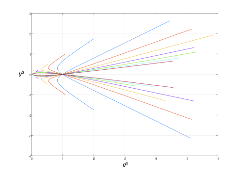
Figure 1. Geodesics starting from $(1,0)$ in the domain $\theta^{1}\pm\theta^{2}>0$.

4. $\alpha$-parallel prior

Takeuchi and Amari [18] studies the invariant $\alpha$-parallel priors with respect to statistical manifolds. Our statistical manifold $M$ given by (3.1) is $\pm 1$-flat, and is hence statistically equiaffine, i.e.,

(4.1) $$\partial_{i}T_{jk}^{k}=\partial_{j}T_{ik}^{k},\quad i,j=1,2,$$

holds everywhere in $M$, where $T_{ij}^{k}=T_{ijl}g^{lk}$. Consequently, $M$ admits $\alpha$-parallel prior $\omega^{(\alpha)}(\theta)$ for any $\alpha\in\mathbb{R}$, satisfying

(4.2) $$\partial_{i}\omega^{(\alpha)}(\theta)=\Gamma_{ij}^{(\alpha)j}\omega^{(\alpha)}(\theta).$$

For the exponential family $M$, this can be simply solved, yielding

(4.3) $$\omega^{(\alpha)}(\theta)=\left(\det G\right)^{(1-\alpha)/2},$$

where $G$ is the Fisher matrix (3.7). In particular, Jeffreys prior (e.g., [8]) is the $0$-prior, while the left-invariant Haar measure (e.g., [19]) is the $-1$-prior.

For a series of independent observations $\mathbf{x}=\{x_{1},x_{2},\ldots,x_{N}\}$ from the beta-logistic distribution (2.22) with unknown parameters $\theta^{1},\theta^{2}$, the posterior distribution $p_{\alpha}(\theta^{1},\theta^{2}\mid\mathbf{x})$ can be obtained by employing (4.3) as the improper prior. From Bayes’ theorem, we have

(4.4) $$p_{\alpha}(\theta^{1},\theta^{2}\mid\mathbf{x})=\frac{p(\mathbf{x};\theta^{1},\theta^{2})\left(\det G\right)^{(1-\alpha)/2}}{A(\mathbf{x})},$$

where

(4.5) $$A(\mathbf{x})=\int_{0}^{\infty}\int_{-\theta^{1}}^{\theta^{1}}p(\mathbf{x};\theta^{1},\theta^{2})\left(\det G\right)^{(1-\alpha)/2}\operatorname{d}\!\theta^{2}\operatorname{d}\!\theta^{1}.$$

The joint distribution of the observations $\mathbf{x}$ is

(4.6) $$p(\mathbf{x};\theta^{1},\theta^{2})=\prod_{i=1}^{N}p(x_{i};\theta^{1},\theta^{2})=\frac{2^{N(1-\theta^{1})}\left(a(\mathbf{x})\right)^{\theta^{1}}\exp(\theta^{2}b(\mathbf{x}))}{B^{N}\left(\frac{\theta^{1}-\theta^{2}}{2},\frac{\theta^{1}+\theta^{2}}{2}\right)},$$

where

(4.7) $$a(\mathbf{x})=\prod\limits_{i=1}^{N}\sech(x_{i}),\quad b(\mathbf{x})=\sum\limits_{i=1}^{N}x_{i}.$$

The maximum a posteriori estimation for the parameters $\theta=(\theta^{1},\theta^{2})$ can hence be obtained by

(4.8) $$\widehat{\theta}=\underset{\theta}{\arg\max}~{}~{}p_{\alpha}(\theta^{1},\theta^{2}\mid\mathbf{x}).$$

Introduce natural logarithm of the posterior distribution (4.4)

(4.9) $$l_{\alpha}(\theta^{1},\theta^{2}\mid\mathbf{x}) =\log p_{\alpha}(\theta^{1},\theta^{2}\mid\mathbf{x})$$

$$=N(1-\theta^{1})\log 2+\theta^{1}\log a(\mathbf{x})+\theta^{2}b(\mathbf{x})-N\log B\left(\frac{\theta^{1}-\theta^{2}}{2},\frac{\theta^{1}+\theta^{2}}{2}\right)$$

$$\quad+\frac{1-\alpha}{2}\log\det G-\log A(\mathbf{x}),$$

where determinant of the Fisher matrix is (see eq. (3.9))

(4.10) $$\det G=4\left(\psi^{\prime}\left(\frac{\theta^{1}-\theta^{2}}{2}\right)\cdot\psi^{\prime}\left(\frac{\theta^{1}+\theta^{2}}{2}\right)-\psi^{\prime}(\theta^{1})\left(\psi^{\prime}\left(\frac{\theta^{1}-\theta^{2}}{2}\right)+\psi^{\prime}\left(\frac{\theta^{1}+\theta^{2}}{2}\right)\right)\right),$$

and the maximum a posteriori estimation $\widehat{\theta}$ can be determined by $\nabla l_{\alpha}=0$, where $\nabla$ denotes the gradient with respect to $\theta$. These equations can be obtained by direct calculation, which read

(4.11) $$\log\frac{a(\mathbf{x})}{2^{N}}-\frac{N}{2}\left(\psi\left(\frac{\theta^{1}+\theta^{2}}{2}\right)+\psi\left(\frac{\theta^{1}-\theta^{2}}{2}\right)-2\psi(\theta^{1})\right)+\frac{1-\alpha}{2}\frac{\partial_{\theta^{1}}\!\det G}{\det G} =0,$$

$$b(\mathbf{x})-\frac{N}{2}\left(\psi\left(\frac{\theta^{1}+\theta^{2}}{2}\right)-\psi\left(\frac{\theta^{1}-\theta^{2}}{2}\right)\right)+\frac{1-\alpha}{2}\frac{\partial_{\theta^{2}}\!\det G}{\det G} =0.$$

Here, we used the properties

(4.12) $$B(x,y)=B(y,x)\text{ and }\partial_{x}B(x,y)=B(x,y)(\psi(x)-\psi(x+y)).$$

Solving the system (4.11) analytically proves to be challenging. Numerical methods can be utilised in practical applications, such as Newton’s method, gradient descent, and fixed-point iteration.

5. Conclusion

Inspired by the probabilistic interpretation of Bernoulli and Euler polynomials as moments of certain distributions, we study the exponential generalized beta of the second distribution, which includes both Bernoulli and Euler cases as special evaluations. Besides the geometric structure, e.g., Fisher information metric, $\alpha$-connection coefficients, $\alpha$-curvature tensors, $\alpha$-Ricci curvature, and the $\alpha$-scalar curvature, we also provide the geodesic equations, which imply that the geodesic spread is at least linearly unstable. Finally, as the statistical manifold is $\pm 1$-flat and hence equiaffine, we give the $\alpha$-parallel prior and the equations determining the maximum a posteriori estimation. Some future work include analytic and numerical solutions to those differential equations, though the former seems to be challenging.

Acknowledgement. L. Peng was partially supported by JSPS KAKENHI grant number JP20K14365, JST-CREST grant number JPMJCR1914, the Fukuzawa Fund and KLL of Keio University.

References

- [1] S. Amari and H. Nagaoka, Methods of Information Geometry, Transl. Math. Monogr., vol 191, Oxford University Press, Oxford, 2000.
- [2] W. D. Baten, The probability law for the sum of independent variables, each subject to the law , Bull. Am. Math. Soc. 40 (1934), 284–290.
- [3] A. Dixit, V. H. Moll, and C. Vignat, The Zagier modification of Bernoulli numbers and a polynomial extension. Part I, Ramanujan J. 33 (2014), 379–422.
- [4] M. P. do Carmo, Riemannian Geometry, Birkhäuser, Boston, 1992.
- [5] M. J. Fischer, Generalized Hyperbolic Secant Distributions: With Applications to Finance, Springer, 2014.
- [6] R. A. Fisher, On the “Probable Error” of a coefficient of correlation deduced from a small sample volume I., Metron 4 (1921), 3–32.
- [7] W. L. Harkness and M. L. Harkness, Generalized hyperbolic secant distributions, J. Amer. Statist. Assoc. 63 (1968), 329–337.
- [8] H. Jeffreys, Theory of Probability, 3rd ed., Oxford University Press, Oxford, 1998.
- [9] L. Jiu, V. H. Moll, and C. Vignat, Identities for generalized Euler polynomials, Integral Transforms Spec. Funct. 25 (2014), 777–789.
- [10] M. Li, H. Sun, and L. Peng, Fisher–Rao geometry and Jeffreys prior for Pareto distribution, Commun. Stat. Theory Methods 51 (2022), 1895–1910.
- [11] W. Magnus, F. Oberhettinger, and F. G. Tricomi, Tables of Integral Transforms. Vol. I., Bateman Manuscript Project, McGraw-Hill, New York, 1954.
- [12] F. W. J. Olver et al. (eds.), NIST Handbook of Mathematical Functions, Cambridge University Press, New York, 2010. Online version: http://dlmf.nist.gov.
- [13] L. Peng, H. Sun, D. Sun, and J. Yi, The geometric structures and instability of entropic dynamic models, Adv. Math. 227 (2011), 459–471.
- [14] W. Perks, On some experiments in the graduation of mortality statistics, J. Inst. Actuar. 63 (1932), 12–57.
- [15] J. Pitman and M. Yor, Infinitely divisible laws associated with hyperbolic functions, Canad. J. Math. 55 (2003), 292–330.
- [16] S. Roman, The Umbral Calculus, Pure and Applied Mathematics, vol. 111, Academic Press Inc., London, 1983.
- [17] H. Sun, Z. Zhang, L. Peng and X. Duan, An Elementary Introduction to Information Geometry, Science Press, Beijing, 2016.
- [18] J. Takeuchi and S. Amari, -parallel prior and its properties, IEEE Trans. Inform. Theory 51 (2005), 1011–1023.
- [19] J. V. Zidek, A representation of Bayesian invariant procedures in terms of Haar measure, Ann. Inst. Statist. Math. 21 (1969), 291–308.