M-Estimation in Censored Regression Model using Instrumental Variables under Endogeneity

Abstract

We propose and study M-estimation to estimate the parameters in the censored regression model in the presence of endogeneity, i.e., the Tobit model. In the course of this study, we follow two-stage procedures: the first stage consists of applying control function procedures to address the issue of endogeneity using instrumental variables, and the second stage applies the M-estimation technique to estimate the unknown parameters involved in the model. The large sample properties of the proposed estimators are derived and analyzed. The finite sample properties of the estimators are studied through Monte Carlo simulation and a real data application related to women’s labor force participation.

Key Words: M-estimation, Tobit model, endogeneity, control variables, two-stage estimation, exogenous variable, instrumental variables.

1 Introduction

The regression models in which the dependent variable is censored or limited to a specific range are referred to as censored regression models. Censoring in a regression model may arise due to the process that generates the data, or it may be incorporated into the model by the experimenter. For instance, expenditure on durable goods may be zero for some households based on their economic status; on the other side, an experimenter may introduce censoring in the data by top-coding the income exceeding a certain level. The first type of censoring in the preceding example is due to the underlying process generating the data, that is, the individual’s decision not to spend on durable goods, while the second type of censoring is independent of the individual’s decision. Tobit models are a particular class of censored regression models where the dependent variable is censored above or below the threshold zero. They are also referred to as standard Tobit models or Tobit type-I models. Tobit models were introduced in the pioneering work by [53] in which Tobin analyzed the household expenditure on durable goods using a regression model with a dependent variable (household expenditure), which was censored below the threshold zero. In this context, the methodology proposed in the Section 2 can be implemented for the non-zero threshold as well.

In this article, we consider Tobit models with endogenous explanatory variables. An explanatory variable is said to be endogenous if it is correlated with the error term in the model. Censoring and endogeneity occur in tandem in many real-life situations. One such real-life example comes from the standard labor supply model, which assumes that each individual has some desired hours of work, say $y^{*}$, which is subject to the constraints of how many hours an individual wants and does not want to work. Thus, the variable $y^{*}$ is assumed to be the interior solution to a utility maximization problem subject to constraints on the number of working hours and leisure. Further, it is also assumed that the firm sets the lower limit of working hours, say $c$. Therefore, the dependent variable $y$ is the actual number of hours worked, which is denoted as $y=y^{*}$ if $y^{*}>c$, and $y=c$ if $y^{*}<c$. In this model, one is interested in examining the effects of other independent variables, such as non-labor income, education, age, wage, etc., on the dependent variable $y$. Therefore, one can fit a regression model to see the effect of these independent variables on $y$. However, it is usually understood that wages and the number of hours are correlated across individuals, which causes the problem of endogeneity in the regression model due to the reverse causality between wages and the number of hours. Now, since the dependent variable $y$ is censored below 0 and there is one endogenous explanatory variable, i.e., wage, in the model, it leads to the problem of estimating the censored regression model with an endogenous explanatory variable.

There are various solutions available in the literature to deal with endogeneity in the Tobit models (see, e.g., [25]). Among them, we consider the instrumental variable (IV) estimation method using the control function approach to remove endogeneity from the model. The instrumental variable method is a standard procedure to remove endogeneity from the model (see, e.g., [8]). This method introduces instrumental variables or instruments, which are correlated,in limit, with the endogenous explanatory variables and uncorrelated,in limit, with the errors in the model. Using the instrumental variables, we consider a two-stage estimation procedure to have some appropriate estimators of the unknown parameters involved in the model. In the first stage, we regress endogenous variables on instrumental variables to find residuals, which are referred to as control variables. In the second stage, we include these control variables as additional explanatory variables to remove the endogeneity from the model under certain assumptions and then estimate the model with M-estimation. An advantage of using the M-estimation procedures with the control function approach to address the issue of endogeneity is that it allows one to include instrumental variables straightforwardly due to its flexibility in specifying the objective function.

1.1 Literature review

Early literature on the estimation of the unknown parameters involved in the Tobit model uses the maximum likelihood estimation technique, assuming the normality of the errors in the model. Later on, [2] established the consistency and asymptotic normality of the maximum likelihood estimator under the assumption that errors are normally distributed, and [24] extended the least squares estimation to a two-step estimation procedure for the Tobit model. The assumption of normality of error is crucial for the estimator to be consistent, unlike in the standard linear regression model, where the parameter estimates are consistent for a wide class of non-normal error distributions. However, if the assumption of normality is violated, then the parameter estimates are inconsistent for the Tobit models; see [22] and [6], where the inconsistency of maximum likelihood estimates was demonstrated for several standard non-normal error distributions. Another important aspect was highlighted by [31], [39], [5], where it is shown that heteroskedasticity of the error terms can also lead to inconsistent parameter estimates even when the functional form of the error density is appropriately specified. The ideas of [40], [10], [26], and [20] are examples of a class of estimation methods that combine likelihood-based approaches with the nonparametric estimation of the distribution function of the error, but this methodology is sensitive to the assumption of identically distributed error terms.

The semi-parametric and non-parametric approaches to estimation have also been introduced to overcome the issue of the specification of error distributions. [45] extends the consistent least absolute deviation (CLAD) estimator to the Tobit model and establishes consistency and asymptotic normality of the estimators without assuming any functional form of the error. However, consistency and asymptotic normality of estimators require stronger assumptions on the behavior of the regression function than those imposed on a model with normally distributed error. In a similar spirit, [46] proposed the symmetrically trimmed least square estimator and established the consistency and asymptotic normality of the estimator, assuming the errors are coming from a symmetric distribution. The modified version of the Huber estimator ([29]) was proposed by [38] for the Tobit models, and it was named as winsorized mean estimators (WME).

It is well known that the use of M-estimation techniques helps in overcoming the robustness issues with the least squares approach ([30]; [23]) for uncensored data. [47], [57], [37] constructed M-estimators for the model using appropriately censored data. The methods described in [47] and [37] are extensions of the estimators proposed by [10] to general M-estimators. All these estimators are consistent and asymptotically normal under some conditions. Although the existence of a solution to the estimating equation has been demonstrated, this approach’s main drawback is that it neither provides a unique solution nor guarantees the consistency of all solutions. [33] developed an M-estimator for the semi-parametric linear model with right-censored data. A class of asymptotically normal, consistent estimators is provided by [33]’s method, which was developed for random censoring. After a few years, [32] developed generalized M-estimators for type-I Tobit models in high-dimensional settings and established consistency and asymptotic normality. Besides, there is an extensive amount of study in the literature addressing the problem of endogeneity in the Tobit models. Early literature relies on complete models with parametric specifications, as studied in [25], [3], [52]. These procedures are primarily based on control function approaches and marginal or conditional maximum likelihood procedures. The semi-parametric approach using the control function is studied by [15], [8], [13].

The instrumental variable estimation provides a consistent estimator of the regression coefficients in the linear model when the random error is correlated with the explanatory variables. The area of instrumental variables has remained an area of interest for many researchers from various perspectives, including parametric, semi-parametric, nonparametric, Bayesian, and non-Bayesian inference. An excellent overview of instrumental variable models is available in [9]. The robust estimation of instrumental variable models has been discussed in the literature by several researchers. A robust instrumental variable estimator is proposed by Cohen et al. (2013). The robustness-related issues of estimators are studied in [54]. The aspect of the robustness of bootstrap inference methods for instrumental variable regression models by considering the test statistics for parameter hypotheses based on the instrumental variables and the generalized method of trimmed moments estimators are discussed in [11]. The Bayesian nonparametric instrumental variables approach to correcting the endogeneity bias in regression models when the functional form of the covariate effects is unknown is discussed in [56]. The aspects of the application of two-stage instrumental variable estimation have been extensively used in real data. For example, [17] presented a goodness of fit statistics in the instrumental variables model and applied it to COVID-19 data; see also [4], [12],[1],[35],[21],[16],[43], [51] etc.

1.2 Main Contribution

In this study, we propose a general class of estimators, which are obtained by applying the M-estimation procedure to a generic loss function $\rho$. One of the advantages of the M-estimation procedure is that it provides flexibility in choosing the objective function, which allows one to customize the estimation procedure according to the complexity of the data and the questions of the research at hand. This adaptability of objective functions can be helpful when some of the classical assumptions of the regression models are violated or there are outliers in the data. One such example can be quantile-based methodology (see, e.g., [18]), which is a particular case of M-estimation-based methodology. We establish consistency and asymptotic normality of the derived estimator under the assumption that $\rho$ is Lipschitz continuous, having the second-order sub-gradient to be bounded. The theoretical results in this paper are established under the same assumption on the behavior of the regression function, as in [45] and [38]. Thus, we bring many standard semi-parametric estimators, such as CLAD and WME, under the same umbrella through a generic loss function and also introduce another estimator by choosing the log cos hyperbolic (log-cosh) loss function. The log-cosh-loss function possesses an important property, as described in [50] that the log-cosh-loss function belongs to the class of robust estimators that focus on solutions near the median rather than the mean. Another point of view is that robust estimators are more tolerant of outliers in the data set, which is possibly one of the main reasons to prefer the log-cosh loss function over others. As demonstrated in the simulation study, the proposed estimator based on the log-cosh loss function performs equally well as the well-known estimators CLAD and WME.

The M-estimators in lower dimensions have not yet been established for censored regression models when data are censored by a fixed constant. Furthermore, models with fixed censoring are more prone to distributional misspecification because knowledge of the underlying data-generating mechanism is seldom available. To get around this, we establish a unified class of estimators with no distributional assumptions and establish consistency and asymptotic normality.

1.3 Overcoming Mathematical Challenges

One of the main challenges is that the objective function may not be continuously differentiable; therefore, usual approaches based on Taylor’s expansion of objective functions are not always applicable. To overcome this problem, we adopt the same technique discussed in [45] with appropriate modifications for a generic Lipschitz continuous loss function. [45] modified the techniques in [28] for the censored outcomes, which approximate the sub-gradient of the objective function by its continuously differentiable expectation. Then, it relates it to the first-order condition, which minimizes the objective function by setting the sub-gradient of the objective function equal to zero asymptotically. We extend regularity conditions to those described in [45] for a class of loss functions to establish consistency and asymptotic normality.

1.4 Organisation of the Paper

The model description is presented in Section 2. Section 2.2 describes the estimation using the control function approach and the proposed M-estimation procedure. Section 3 presents the main theoretical results and states the main theorems. Section 4 provides a simulation study to validate the theoretical results. Section 5 showcases real-life applications of the proposed methodology on a real data set. Finally, Section 6 provides some concluding remarks on this work. All the proofs of the theorems are supplied in Section 7.

The R codes of simulated and real data study are available at https://github.com/swati-1602/CRM.git.

2 Model Description and Estimation Procedure

2.1 The Model

For given paired data $(y_{i},\boldsymbol{x}^{*}_{i}),\hskip 2.84544pti=1,\ldots,n,$ where $y_{i}$ is the $i^{th}$ observations on the response variable, defined as

$$y_{i}=\begin{cases}y^{*}_{i}&\text{if}\>y^{*}_{i}>\textit{c}\\ \textit{c}&\text{if}\>y^{*}_{i}\leq\textit{c},\\ \end{cases}$$

where $c$ is a fixed and non-random censoring threshold. Here $y_{i}$ is fully observed but the latent variable $y_{i}^{*}$ is not fully observed and modelled as

$$y^{*}=\boldsymbol{x}^{T}_{i}\boldsymbol{\alpha}_{0}+w_{i}\gamma_{0}+\epsilon_{i},$$ (2.1)

and $\boldsymbol{x}^{*}_{i}=(\boldsymbol{x}_{i},w_{i})$ is the $i^{th}$ observations on a vector of $(p+1)$ dimensional explanatory variables with two components. One component $\boldsymbol{x}_{i}=(x_{i1},\ldots,x_{ip})^{T}$ is a vector of $p$ dimensional exogenous explanatory variables that are uncorrelated with the error term, and $w_{i}$ is the endogenous explanatory variable that is correlated with the error term in (2.1). The unobservable random error $\epsilon_{i}$ is assumed to be independent of $\boldsymbol{x}_{i}$. Here, we have considered only one endogenous variable in the model for the sake of simplicity in understanding. However, the results and estimation procedure in this paper are also applicable and can be extended to a model with more than one endogenous variable. The vector of unknown parameters associated with the exogenous variable is denoted by $\boldsymbol{\alpha}_{0}=(\alpha_{10},\ldots,\alpha_{p0})^{T}$ and the parameter associated with the endogenous explanatory variable is represented by $\gamma_{0}$.

Now, consider the censored linear regression model with left censoring at a fixed and non-random threshold $c$, also called the standard Tobit model, defined as

$$y_{i}=\max\leavevmode\nobreak\ (c,y^{*})=\max\leavevmode\nobreak\ \{c,\boldsymbol{x}^{T}_{i}\boldsymbol{\alpha}_{0}+w_{i}\gamma_{0}+\epsilon_{i}\},\hskip 11.38092pti=1,\ldots,n.$$ (2.2)

This model is often referred to as the semi-parametric censored linear regression model since the error distribution is not specified. Without loss of generality, we restrict our study to a censored linear regression model where the censoring threshold is 0, i.e.,

$$y_{i}=\text{ max }\{0,\boldsymbol{x}^{T}_{i}\boldsymbol{\alpha}_{0}+w_{i}\gamma_{0}+\epsilon_{i}\},\hskip 2.84544pti=1,\ldots,n.$$ (2.3)

2.2 Estimation of Parameters in Presence of Endogeneity

The common approach to estimating the parameters of a regression model in the presence of one or more endogenous regressors is based on the instrumental variable (IV) approach. The instrumental variable approach is based on the principle that, in the first stage, the endogeneity from the model is removed with the help of instruments or instrumental variables. Then, one estimates the parameters of the model in the next stage using some suitable estimation technique. The inherent assumption in the instrumental variable approach is the validity of the instruments. An instrument is said to be valid if it is exogenous and is correlated with the endogenous variables. In the present context, we use instrumental variable estimation based on the control function approach (see, e.g., [52], [41], and [48]) to remove endogeneity from the model.

Let $z_{i}$ denote the $i^{th}$ value of the instrumental variable corresponding to the endogenous variable $w_{i}$ in the model (2.3), for $i=1,\ldots,n$. Then the control function approach proceeds in the following steps:

1. We regress the observations on endogenous variable $w_{i}$ on the instrumental variable $z_{i}$, i.e.,

   $$w_{i}=z_{i}\delta_{1}+\eta_{i},\quad i=1,\ldots,n,$$ (2.4)

   where $\delta_{1}$ is the unknown parameter associated with $z$ and $\eta_{i}$ is the random error in the $i^{th}$ observation such that $cov(z_{i},\eta_{i})=0$.

2. The source of endogeneity is controlled using $E(\epsilon_{i}|\eta_{i})$ by decomposing $\epsilon_{i}$ as follows:

   $$\epsilon_{i}=E(\epsilon_{i}|\eta_{i})+\xi_{i},\quad i=1,\ldots,n,$$ (2.5)

   where $\xi_{i}$ is a random variable denoting the deviation of $\epsilon_{i}$ from $E(\epsilon_{i}|\eta_{i})$. Note that $E(\epsilon_{i}|\eta_{i})\neq 0$ since $w_{i}$ is endogenous, implying that $cov(\epsilon_{i},\eta_{i})\neq 0$.

3. The control function is the functional form of $E(\epsilon_{i}|\eta_{i})$, which is often chosen to be linear, and we choose $E(\epsilon_{i}|\eta_{i})=\rho_{10}\eta_{i}$, reducing (2.5) as follows:

   $$\epsilon_{i}=\rho_{10}\eta_{i}+\xi_{i},\quad i=1,\ldots,n,$$ (2.6)

   where $\rho_{10}$ is an unknown parameter in (2.6).

4. The idea is to incorporate the control function in the original model (see, (2.3)) to account for endogeneity and use $\xi_{i}$ as the error term instead of $\epsilon_{i}$. Note that (2.5) is constructed in such a way that $cov(\xi_{i},\eta_{i})=0$, since all the variation in $\epsilon_{i}$ due to $\eta_{i}$ is subsumed into $E(\epsilon_{i}|\eta_{i})$. Thus, the following transformed model will be free from endogeneity and can be estimated using any suitable technique.

   $$y_{i}=\text{ max }\{0,\boldsymbol{x}^{T}_{i}\boldsymbol{\alpha}_{0}+w_{i}\gamma_{0}+\rho_{10}\eta_{i}+\xi_{i}\},\quad i=1,\ldots,n.$$ (2.7)

5. The model in (2.7) contains $\eta_{i}$, which is unobserved. Therefore, we replace $\eta_{i}$ by the residuals of the model in (2.4). Let $e_{i},i=1,\ldots,n$ denote the residuals of the model in (2.4), then the model in (2.7) becomes

   $$y_{i}=\text{ max }\{0,\boldsymbol{x}^{T}_{i}\boldsymbol{\alpha}_{0}+w_{i}\gamma_{0}+e_{i}\rho_{10}+\xi_{i}\}=\text{ max }\{0,\boldsymbol{X}^{T}_{i}\boldsymbol{\beta}_{0}+\xi_{i}\},$$ (2.8)

   where $\boldsymbol{X}_{i}=[\boldsymbol{x}_{i},w_{i},e_{i}]^{T}$ and $\boldsymbol{\beta}_{0}=[\boldsymbol{\alpha}_{0},\gamma_{0},\rho_{10}]^{T}$ is the $m\times 1$ vector of unknown parameters with $m=p+2$.

2.2.1 Implementation of M-estimation Technique

The parameters of the model described in (2.8) can be estimated using any suitable estimation procedure, such as censored least absolute deviation (CLAD) ([45]) and winsorized mean estimator (WME) ([38]), to name a few. In this article, we take a general perspective using a general loss function, which encapsulates some existing estimation procedures, such as CLAD and WME as its particular cases. We use the well-known estimation procedure, the M-estimation procedure, to estimate the parameters in (2.8). The definition of such an estimator, denoted as $\hat{\boldsymbol{\beta}}_{n}$, is as follows:

$$\hat{\boldsymbol{\beta}}_{n}=\underset{\boldsymbol{\beta}\in\mathcal{B}}{\arg\min}\leavevmode\nobreak\ Q_{n}(\boldsymbol{\beta}),$$ (2.9)

where

$$Q_{n}(\boldsymbol{\beta})=\frac{1}{n}\sum_{i=1}^{n}\rho(y_{i},\boldsymbol{\beta})=\frac{1}{n}\sum_{i=1}^{n}\rho(y_{i}-\text{ max }\{0,\boldsymbol{X}^{T}_{i}\boldsymbol{\beta}\}).$$ (2.10)

Here $\boldsymbol{\beta}=(\boldsymbol{\alpha},\gamma,\rho_{1})^{T},$ $\mathcal{B}$ is the parameter space of $\boldsymbol{\beta},$ and $\rho$ is a real valued loss function. If $\rho$ in (2.10) is differentiable in $\boldsymbol{\beta}$ with a continuous derivative $\frac{\partial\rho(y_{i},\boldsymbol{\beta})}{\partial\boldsymbol{\beta}}$ then, $\hat{\boldsymbol{\beta}}_{n}$ is a root of the equation

$$\frac{1}{n}\sum_{i=1}^{n}\frac{\partial(\rho(y_{i},\boldsymbol{\beta}))}{\partial\boldsymbol{\beta}}=0,\hskip 14.22636pt\boldsymbol{\beta}\in\mathcal{B.}$$ (2.11)

The class of M-estimators covers the following well-known estimators for the Tobit model for a given choice of $\rho$:

1. The censored least absolute deviation estimator (CLAD) corresponds to

   $$\rho(y_{i},\boldsymbol{\beta})=|(y_{i}-\text{ max }\{0,\boldsymbol{X}^{T}_{i}\boldsymbol{\beta}\}|.$$ (2.12)

2. The winsorized mean estimator (WME) corresponds to

   $$\rho(y_{i},\boldsymbol{\beta})=\begin{cases}\frac{1}{2}\left(y_{i}-\text{ max }\{0,\boldsymbol{X}^{T}_{i}\boldsymbol{\beta}\}\right)^{2},&\text{if }|y_{i}-\text{ max }\{0,\boldsymbol{X}^{T}_{i}\boldsymbol{\beta}\}|\leq w\\ w\left(|y_{i}-\text{ max }\{0,\boldsymbol{X}^{T}_{i}\boldsymbol{\beta}\}|-\frac{w}{2}\right),&\text{otherwise.}\end{cases}$$ (2.13)

3. The censored log cosh estimator (CLCE) corresponds to

   $$\rho(y_{i},\boldsymbol{\beta})=log(cosh(y_{i}-\text{max}(0,\boldsymbol{X}^{T}_{i}\boldsymbol{\beta}))).$$ (2.14)

3 Asymptotic Properties of $\hat{\boldsymbol{\beta}}_{n}$

There is a vast literature on the asymptotic properties, such as consistency and asymptotic normality, of M-estimators for the usual regression model. However, to the best of our knowledge, we are unaware of any literature on the asymptotic properties of M-estimators for regression models when the response variable is censored at a non-random and fixed threshold in the presence of endogeneity. In this article, we establish the consistency and asymptotic normality of $\hat{\boldsymbol{\beta}}_{n}$ described in (2.9).

One of the major issues in applying the M-estimation technique to the model described in (2.3) is that the objective function need not be convex and differentiable. The non-convexity of the objective function $Q_{n}(\boldsymbol{\beta})$ (see, (2.10)) poses the problem of non-identifiability of the true parameter $\boldsymbol{\beta}_{0}$. For example, consider the case when all the observations are censored, that is, $y_{i}=0\;\text{for all}\;i=1,\ldots,n$. Then we have,

$$Q_{n}(\boldsymbol{\beta})=\frac{1}{n}\sum\limits_{i=1}^{n}\rho(-max\{0,\boldsymbol{X}^{T}_{i}\boldsymbol{\beta}\}).$$

In such a case, $Q_{n}(\boldsymbol{\beta})=0$ for any $\boldsymbol{\beta}\in\mathcal{B}$ for which $\boldsymbol{X}^{T}_{i}\boldsymbol{\beta}\leq 0$ for all $i=1,\ldots,n$, under the assumption that $\rho(0)=0$ (see $\boldsymbol{A.4}$ in Section 3.1). Therefore, assuming $\rho$ to be a non-negative loss function, any value $\boldsymbol{\beta}\in\mathcal{B}$ for which $\boldsymbol{X}^{T}_{i}\boldsymbol{\beta}\leq 0$ for all $i=1,\ldots,n$, is a minimizer of $Q_{n}(\boldsymbol{\beta})$. Thus, $\hat{\boldsymbol{\beta}}_{n}$ is not unique, and the true parameter $\boldsymbol{\beta}_{0}$ is not identifiable in this case.

To avoid the above-mentioned situation, one can assume that there are “enough” numbers of uncensored observations for a large sample size of $n$. More precisely, let $n_{0}$ denote the number of uncensored observations in a sample of size $n$ such that $n_{0}/n\xrightarrow{}\lambda\in(0,1]$ as $n\xrightarrow{}\infty$. In this case, for any $\boldsymbol{\beta}\in\mathcal{B}$ for which $\boldsymbol{X}^{T}_{i}\boldsymbol{\beta}\leq 0$ for all $i=1,\ldots,n$, we have,

$$Q_{n}(\boldsymbol{\beta})=\frac{1}{n}\sum\limits_{i=1}^{n_{0}}\rho(y_{i}).$$

Note that for this case as well, one encounters the problem related to the non-identifiability of $\boldsymbol{\beta}_{0}$ since $Q_{n}(\boldsymbol{\beta})$ does not depend on $\boldsymbol{\beta}$. As a consequence, any $\boldsymbol{\beta}\in\mathcal{B}$ for which $\boldsymbol{X}^{T}_{i}\boldsymbol{\beta}\leq 0$ for all $i=1,\ldots,n$, is a minimizer of $Q_{n}(\boldsymbol{\beta})$. This again leads to the problem of the non-identifiability of $\boldsymbol{\beta}_{0}$ and the non-uniqueness of $\hat{\boldsymbol{\beta}}_{n}.$

In light of both the above-described situations, it is necessary to restrict that $\boldsymbol{X}^{T}_{i}\boldsymbol{\beta}>0$ for “enough” observations in a large sample. Therefore, minimization of (2.9) can be viewed as executing M-estimation only for those sample observations for which $\boldsymbol{X}^{T}_{i}\boldsymbol{\beta}\geq 0$. Thus, if $\hat{\boldsymbol{\beta}}_{n}$ is to be consistent, the true regression function $\boldsymbol{X}^{T}_{i}\boldsymbol{\beta}_{0}$ must be non-negative for a significant proportion of the sample. As pointed out in [45], to overcome the issue of non-identifiability of $\boldsymbol{\beta}_{0}$, it is necessary to restrict the behavior of the true regression function $\boldsymbol{X}^{T}_{i}\boldsymbol{\beta}_{0}$ such that for large enough samples $\boldsymbol{X}^{T}_{i}\boldsymbol{\beta}_{0}>0$, and the regressors are not collinear. This requirement is articulated in the assumption $\boldsymbol{A.3}$.

3.1 Strong Consistency of $\hat{\boldsymbol{\beta}}_{n}$

We establish the consistency of $\hat{\boldsymbol{\beta}}_{n}$ under the following assumptions on the parameter space, errors, regressors, the true regression function, and the loss function. Recall the model (2.8); all of the assumptions discussed below are based on it.

Assumptions:

1. $\mathcal{B}$ defined in (2.9) and (2.10) is a compact space, and $\boldsymbol{\beta}_{0}\in\mathcal{B}^{o}.$ Here $\boldsymbol{\beta}_{0}$ is the same as defined in (2.8), and $\mathcal{B}^{o}$ is the interior of $\mathcal{B}.$

2. The random variables $\{\xi_{i}\}_{1\leq i\leq n}$ defined in (2.5) are identically and independently distributed with the common probability density function $f$. Moreover, for all $1\leq i\leq n,$ $\xi_{i}$ is independent of $\boldsymbol{X}_{i},$ where $\boldsymbol{X}_{i}$ is the same as defined in (2.8).

3. For all $1\leq i\leq n,$ the random vectors $\{\boldsymbol{X}_{i}\}$ defined in (2.8) are independent with $E\|\boldsymbol{X}_{i}\|^{4}<K_{0},$ where $K_{0}$ is some positive constant. Moreover, for some positive $\epsilon_{0}>0,$

   $$\underset{n\to\infty}{\lim}E\left[\frac{1}{n}\sum_{i=1}^{n}\mathds{1}(\boldsymbol{X}_{i}^{T}\boldsymbol{\beta}_{0}\geq\epsilon_{0})\boldsymbol{X}_{i}\boldsymbol{X}^{T}_{i}\right]=Q,$$ (3.1)

   where $Q$ is some positive definite matrix.

4. $\rho(x)\geq 0$ for all $x\in\mathbb{R},$ $\rho(0)=0,$ $\rho(x)=\rho(-x)$ for all $x\in\mathbb{R},$ and moreover,

   $$|\rho(x)-\rho(y)|\leq k.|x-y|,$$

   where $k$ is some positive constant. Here $\rho$ is the same as defined in (2.10).

5. For all ${1\leq i\leq n},$

   $$E[\rho(y_{i}-max(0,\boldsymbol{X}^{T}_{i}\boldsymbol{\beta}_{0}))]<E[\rho(y_{i}-max(0,\boldsymbol{X}^{T}_{i}\boldsymbol{\beta}))].$$ (3.2)

Remark 3.1.

As required by Lemma 7.2, the assumption $\boldsymbol{A.1}$ guarantees the existence and measurability of $\hat{\boldsymbol{\beta}}_{n}$ as well as the uniformity of the almost sure convergence of the minimand over $\mathcal{B}$. Assumption $\boldsymbol{A.2}$ is self-explanatory. Assumption $\boldsymbol{A.3}$ ensures that $\boldsymbol{X}_{i}^{T}\boldsymbol{\beta}_{0}>0$ for ”enough” sample points and the regressors $\boldsymbol{X}_{i}$’s are not collinear for these observations. Assumption $\boldsymbol{A.4}$ implies that the loss function is smooth enough. The condition described in (3.2) is borrowed from [19], which is necessary to ensure the identifiable uniqueness of the true parameter $\boldsymbol{\beta}_{0}$. It is indeed true that such a condition holds for a wide range of $\rho$.

Theorem 3.1.

For the model described in (2.8), under the assumptions $\boldsymbol{A.1}$, $\boldsymbol{A.2}$, $\boldsymbol{A.3}$, $\boldsymbol{A.4}$, and $\boldsymbol{A.5}$, we have $||\hat{\boldsymbol{\beta}}_{n}-\boldsymbol{\beta}_{0}||_{\mathbb{R}^{m}}\rightarrow 0$ almost surely as $n\rightarrow\infty$. Here $m=p+2$, $\hat{\boldsymbol{\beta}}_{n}$ is the same as defined in (2.9), and $\boldsymbol{\beta}_{0}$ is the same as defined in (2.8).

Proof.

See Appendix $B.1.$ ∎

3.2 Asymptotic Normality of $\hat{\boldsymbol{\beta}}_{n}$

In this section, we establish the asymptotic distribution of $\hat{\boldsymbol{\beta}}_{n}$ described in (2.9). Since the sample minimand $Q_{n}(\boldsymbol{\beta})$ is non-differentiable, the common method for proving asymptotic normality, which relies on an expansion of the objective function using Taylor’s expansion, is not immediately applicable to the situation at hand. The purpose of this paper is to establish general asymptotic normality results equivalent to those found in [14], [27], [28], and the following works (see, e.g., [28], [7], [34], [49], [36], [44], and [45]). As the loss function involved in (2.10) is not differentiable at $\boldsymbol{\beta}$ when $\boldsymbol{X}^{T}_{i}\boldsymbol{\beta}=0$, we must rule out sequences of $\boldsymbol{X}_{i}$ values that are orthogonal to $\boldsymbol{\beta}$ and have a positive frequency to establish the asymptotic normality of $\hat{\boldsymbol{\beta}}_{n}$. The following assumption is sufficient for this purpose:

• For some constants, $K_{1}>0$ and $\zeta_{0}>0$, and for all $1\leq i\leq n,$ the random vector $\boldsymbol{X}_{i}$ defined in (2.8), under the condition $\|\boldsymbol{\beta}-\boldsymbol{\beta}_{0}\|<\zeta_{0}$, satisfy the following inequality for all $0\leq z^{*}<\zeta_{0},$ and $r=0,1,2:$

  $$E\left[\mathds{1}\left(|\boldsymbol{X}^{T}_{i}\boldsymbol{\beta}|\leq\|\boldsymbol{X}_{i}\|.z^{*}\right)\|\boldsymbol{X}_{i}\|^{r}\right]\leq K_{1}.z^{*}.$$

• The loss function $\rho$ defined in (2.10) is twice differentiable with respect to $\boldsymbol{\beta}$, provided $\boldsymbol{X}^{T}_{i}\boldsymbol{\beta}>0$ for all $1\leq i\leq n.$ Moreover, for some constants $M_{0}>0$ and $M_{1}>0$, $|\rho^{\prime}(x)|\leq M_{1}$ and $|\rho^{\operatorname*{\prime\prime}}(x)|\leq M_{0}$ for all $x\in\mathbb{R},$ and in addition, $\sum\limits_{i=1}^{\infty}\rho^{\prime}(y_{i}-\boldsymbol{X}^{T}_{i}\boldsymbol{\beta}_{0})<\infty$, almost surely for all $1\leq i\leq n.$ Here $\rho^{{}^{\prime}}$ and $\rho^{{}^{\prime\prime}}$ denote the first and second derivatives of $\rho$, respectively.

Remark 3.2.

The assumption $\boldsymbol{A.6}$ implies the differentiability of the minimand defined in (2.10) at $\boldsymbol{\beta}.$ Further, when for all $1\leq i\leq n$, $\boldsymbol{X}^{T}_{i}\boldsymbol{\beta}>0,$ with probability 1, then $\boldsymbol{A.6}$ holds, under some smoothness condition on the distribution of $\boldsymbol{X}_{i}$. Moreover, the assumption $\boldsymbol{A.7}$ ensures some degree of smoothness of the loss function $\rho$ along with some tail property of the function $\rho.$

Theorem 3.2.

For the model described in (2.8), under the assumptions $\boldsymbol{A.1}$, $\boldsymbol{A.6}$ and $\boldsymbol{A.7}$, we have

$$D_{n}^{-1/2}H_{n}.\sqrt{n}\left(\hat{\boldsymbol{\beta}}_{n}-\boldsymbol{\beta}_{0}\right)\overset{d}{\to}Z,$$

where Z is a $\mathbb{R}^{m}$ valued random vector associated with a standard m-dimensional multivariate normal distribution,

$$H_{n}=\frac{1}{n}\sum_{i=1}^{n}E\left[\mathds{1}\left(\boldsymbol{X}^{T}_{i}\boldsymbol{\beta}_{0}>0\right)\boldsymbol{X}_{i}\boldsymbol{X}^{T}_{i}\rho^{\operatorname*{\prime\prime}}\left(y_{i}-\boldsymbol{X}^{T}_{i}\boldsymbol{\beta}_{0}\right)\right],$$

and $D^{-1/2}_{n}$ is such that

$$(D_{n}^{-1/2}D_{n}^{-1/2})^{-1}=\frac{1}{n}\sum_{i=1}^{n}E\left[\mathds{1}\left(\boldsymbol{X}^{T}_{i}\boldsymbol{\beta}_{0}>0\right)\boldsymbol{X}_{i}\boldsymbol{X}^{T}_{i}\{\rho^{\prime}\left(y_{i}-\boldsymbol{X}^{T}_{i}\boldsymbol{\beta}_{0}\right)\}^{2}\right].$$

Proof.

See Appendix $B.2.$ ∎

3.3 Consistent Estimation of $D_{n}$ and $H_{n}$

Consistent estimators of $D_{n}$ and $H_{n}$ must be derived to use the asymptotic normality of $\hat{\boldsymbol{\beta}}_{n}$ to construct large sample hypothesis tests for the parameter vector $\boldsymbol{\beta}_{0}$. There are “natural” estimators of the matrices $H_{n}$ and $D_{n}$ for the model (2.8); these are

$$\begin{split}\hat{H_{n}}&=\frac{1}{n}\sum_{i=1}^{n}\mathds{1}\left(\boldsymbol{X}^{T}_{i}\hat{\boldsymbol{\beta}}_{n}>0\right)\boldsymbol{X}_{i}\boldsymbol{X}^{T}_{i}\rho^{\operatorname*{\prime\prime}}\left(y_{i}-\boldsymbol{X}^{T}_{i}\hat{\boldsymbol{\beta}}_{n}\right)\\ &=\frac{1}{n}\sum_{i=1}^{n}\mathds{1}\left(\boldsymbol{X}^{T}_{i}\hat{\boldsymbol{\beta}}_{n}>0\right)\boldsymbol{X}_{i}\boldsymbol{X}^{T}_{i}\rho^{\operatorname*{\prime\prime}}\left(\hat{\xi}_{i}\right)\end{split}$$ (3.3)

and

$$\hat{D_{n}}=\frac{1}{n}\sum_{i=1}^{n}\mathds{1}\left(\boldsymbol{X}^{T}_{i}\hat{\boldsymbol{\beta}}_{n}>0\right)\boldsymbol{X}_{i}\boldsymbol{X}^{T}_{i}\{\rho^{\prime}(\hat{\xi_{i}})\}^{2},$$ (3.4)

where, $\hat{\xi_{i}}=y_{i}-\boldsymbol{X}^{T}_{i}\hat{\boldsymbol{\beta}}_{n}.$

Theorem 3.3.

Under the conditions of Theorem 3.2, the estimators $\hat{H}_{n}$ and $\hat{D}_{n},$ as stated in (3.3) and (3.4), are strongly consistent, i.e., $\hat{H}_{n}-H_{n}=o(1)$ and $\hat{D}_{n}-D_{n}=o(1)$ almost surely.

Proof.

See Appendix $B.3.$ ∎

In view of the assertions in Theorems 3.2 and 3.3, we have the following result:

Proposition 3.1.

Under the assumptions in Theorems 3.2 and 3.3, we have

$$\hat{D}_{n}^{-1/2}\hat{H}_{n}.\sqrt{n}\left(\hat{\boldsymbol{\beta}}_{n}-\boldsymbol{\beta}_{0}\right)\overset{d}{\to}Z,$$

where Z is a $\mathbb{R}^{m}$ valued random vector associated with a standard m-dimensional multivariate normal distribution, $\hat{D}_{n}$ and $\hat{H}_{n}$ are the same as defined in (3.4) and (3.3), respectively.

Remark 3.3.

Observe that one may conduct testing of hypothesis problems related to $\boldsymbol{\beta}_{0}$ or construct a confidential interval of $\boldsymbol{\beta}_{0}$ using the result described in proposition in 3.1 as $\hat{D}_{n}$, $\hat{H}_{n}$, and $\hat{\boldsymbol{\beta}}_{n}$ are computable for a given data in principle regardless of the computational complexity.

4 Simulation Study

In this section, Monte Carlo experiments are performed to study the finite sample performance of the estimators in terms of their empirical bias and mean square error (MSE). This section compares the effectiveness of the proposed estimators of the unknown parameters involved in the model (2.8) with an endogenous regressor. In this study, we compare the performance of the estimators defined in Section 2.2.1, namely, CLAD (see, (2.12)), WME (see, (2.13)), and CLCE (see, (2.14)). The following model is considered to generate the data: For $i=1,\ldots,n$,

$$y^{*}_{i} =\beta_{0}+\beta_{1}x_{1i}+\beta_{2}x_{2i}+e_{1i},$$ (4.1)

$$x_{2i} =\alpha z_{i}+e_{2i},$$ (4.2)

$$e_{1i} =\rho_{1}e_{2i}+\eta_{i},$$ (4.3)

$$y_{i} =\text{max}(0,\beta_{0}+\beta_{1}x_{1i}+\beta_{2}x_{2i}+\rho_{1}e_{2i}+\eta_{i}),$$ (4.4)

In the model (4.1), the endogenous regressor $x_{2i}$ is regressed on the instrumental variable $z_{i}$ (see, (4.2)), and the exogenous regressor $(x_{1i})$ is generated from the standard normal distribution $N(0,1)$. The random error $e_{2i}$ corresponding to the model (4.2) are generated from $N(0,1)$, while $z_{i}$ is generated from the uniform distribution over $(0,1)$, i.e., $U(0,1)$. Consequently, the observations on $x_{2i}$ are generated for given values of $\alpha=1$. Let $\beta_{T}=(\beta_{0},\beta_{1},\beta_{2},\rho_{1})=(1,2,3,0.5)$, where $\beta_{T}$ represents the true parameter values. As mentioned in Section 2.2, by applying the control function approach, the random error $e_{1i}$ in the model (4.1) and the random error corresponding to the model (4.2) are correlated (see (4.3)). Afterwards, models (4.1) and (4.2) lead to the model (4.4). The homoscedastic random errors $\eta_{i}$ corresponding to the model (4.4) are generated from the following distributions: standard normal distribution $N(0,1)$, Laplace distribution $DE(0,1)$, and $t$-distribution with $n$ degrees of freedom $t_{n}$. The heteroscedastic errors $\xi_{i}$ are generated from $N(0,\sigma_{X_{i}}^{2})$, where $\sigma_{X_{i}}^{2}=(\boldsymbol{X}^{T}_{i}\boldsymbol{\beta})^{2},\boldsymbol{X_{i}}=(x_{1i},x_{2i})^{T}$ and $\boldsymbol{\beta}=(\beta_{1},\beta_{2})^{T}$. The impact of non-normally distributed random errors on the empirical bias and empirical MSE can be judged by comparing the values from $DE(0,1)$ and $U(0,1)$ with $N(0,1)$. The performance of the proposed estimators studied by considering various choices of the loss function $\rho$, while the distributions of $\eta_{i}$ are kept relatively simple so that the true values of the censored regression coefficients are tractable. Since $\rho$ is a Lipschitz-Continuous function, we consider a least absolute error loss function (see (2.12)), a Huber error loss function with a tuning parameter $w=1.35$ (see (2.13)), and a log-cosh loss function (see (2.14)) as particular choices of $\rho$. Next, the estimated values of $\beta_{0},$ $\beta_{1},$ $\beta_{2}$ and $\rho_{1}$ are computed from the Nelder-Meade simplex algorithm using the “optim” function in R software for these loss functions. We replicate this process $r=5000$ times for the sample size $n\in\{50,100,150,1000\}$. Then, the empirical bias and empirical mean squared error (MSE) of the parameter estimates of $\beta_{0}$, $\beta_{1}$, $\beta_{2}$, and $\beta_{3}=\rho_{1}$ are computed as follows:

$$Bias(\hat{\beta}_{j})=\frac{1}{r}\sum_{k=1}^{r}\left(\hat{\beta}_{jk}-\beta_{j}\right),j=0,1,2,3$$

and

$$MSE(\hat{\beta}_{j})=\frac{1}{r}\sum_{k=1}^{r}\left(\hat{\beta}_{jk}-\beta_{j}\right)^{2},j=0,1,2,3$$

where $\hat{\beta}_{ij}$ is the estimate of the parameter $\beta_{j}$ in the $k^{th},k=1,2,\ldots r$ replicate. For these designs, the overall censoring probabilities vary between $18\%$ to $48\%$, and the different censoring percentages do not change any qualitative conclusions.

Tables 1 and 2 report the empirical bias and empirical mean square error of the proposed estimators along with the probability of censored observations for varying sample sizes $n\in\{50,100,500,1000\}$. Due to keeping the length of the paper shorter, the empirical bias and empirical MSE are reported only for $n\in\{50,100,500,1000\}$. It is clear from the results that estimators corresponding to different $\rho$ give different bias and MSE, which depend on the distribution generating random errors. In all cases, MSEs are decreasing as the sample size increases. Table 1 demonstrates that the bias and MSE of the CLAD, WME, and CLCE estimators are considerably higher for the small sample size in the case of all error distributions. For $n=50$, the MSE of the WME and CLCE estimators is higher than that of CLAD estimates in the case of homoscedastic error. In the case of heteroscedastic error, increasing the variance of the error term does have an adverse impact on CLCE and WME estimators, while CLAD is a better choice in this scenario. For $n=100$, it performs well because these estimators are less sensitive to outliers, and as the sample size increases further, CLCE and CLAD estimators perform well as compared to WME estimators. For the sample size $n=500,1000$, the bias and MSE of the proposed estimators are approaching zero in the case of all error distributions, which is congruous with the fact that the proposed estimators are asymptotically unbiased and consistent.

Table 1: Empirical bias and MSE of $\hat{\beta_{0}},$ $\hat{\beta_{1}},$ $\hat{\beta_{2}}$ and $\hat{\rho_{1}}$ with $n=50,100.$

Estimators	$\boldsymbol{\beta}$	Error-distribution
		$N(0,1)$			$DE(0,1)$			$t_{n}$			$N(0,\sigma_{X_{i}}^{2})$, $\sigma_{X_{i}}^{2}=(\boldsymbol{X}^{T}_{i}\boldsymbol{\beta})^{2}$
		Bias	MSE	C.P	Bias	MSE	C.P	Bias	MSE	C.P	Bias	MSE	C.P
		$n=50$
	$\beta_{0}$	0.1036	0.5342		0.1153	0.6155		0.1165	0.4199		-0.4188	1.9455
CLAD	$\beta_{1}$	0.0009	0.0566	22$\%$	0.0074	0.0615	38$\%$	0.0104	0.0538	26$\%$	0.2362	1.1679	48$\%$
	$\beta_{2}$	-0.2207	1.0975		-0.2653	1.2673		-0.2791	1.6153		0.0458	7.1524
	$\rho_{1}$	0.2363	1.1495		0.2957	1.3139		0.2975	1.6387		-0.2375	6.8123
	$\beta_{0}$	0.0300	2.5824		-0.0089	5.8653		0.0874	5.3688		–2.3589	77.024
WME	$\beta_{1}$	0.0213	0.0568	18$\%$	0.0295	0.0948	24$\%$	0.0143	0.0610	34$\%$	0.5879	6.0178	38$\%$
	$\beta_{2}$	-0.1094	13.863		-0.0547	20.351		-0.2107	20.891		1.3187	184.66
	$\rho_{1}$	0.1411	13.999		0.0990	20.365		0.2411	20.933		-0.0087	176.35
	$\beta_{0}$	0.1500	2.5797		0.1031	2.8856		0.1059	2.5419		-0.4741	53.334
CLCE	$\beta_{1}$	-0.0161	0.0454	30$\%$	-0.0190	0.0589	38$\%$	-0.0078	0.0434	28$\%$	0.1414	1.7814	46$\%$
	$\beta_{2}$	-0.2498	9.1222		-0.1596	11.327		-0.1725	10.190		0.0011	123.23
	$\rho_{1}$	0.2209	9.0952		0.1343	11.252		0.1582	10.210		0.5446	123.18
		$n=100$
	$\beta_{0}$	0.0725	0.3409		0.0817	0.3916		0.0721	0.1807		-0.3198	0.8408
CLAD	$\beta_{1}$	-0.0021	0.0325	25$\%$	0.0038	0.0302	30$\%$	0.0082	0.0209	30$\%$	0.1835	0.4920	28$\%$
	$\beta_{2}$	-0.1597	0.5754		-0.1813	0.9068		-0.1728	0.4896		0.1310	3.1660
	$\rho_{1}$	0.1688	0.5861		0.1900	0.9347		0.1948	0.4963		-0.4250	2.7691
	$\beta_{0}$	0.0054	1.2936		0.0115	0.5094		0.0325	1.4159		-0.9830	10.263
WME	$\beta_{1}$	0.0158	0.0116	29$\%$	0.0147	0.0116	22$\%$	0.0069	0.0238	28$\%$	0.2790	1.4183	26$\%$
	$\beta_{2}$	-0.0419	4.8663		-0.0824	1.2155		-0.0968	4.4673		0.4015	19.363
	$\rho_{1}$	0.0593	4.8618		-0.1116	1.2207		0.1077	4.4372		0.2418	19.371
	$\beta_{0}$	0.0882	0.9985		0.1158	0.4890		0.0945	0.3628		-0.0594	8.4772
CLCE	$\beta_{1}$	-0.0095	0.0139	28$\%$	-0.0219	0.0136	38$\%$	-0.0164	0.0206	25$\%$	0.0162	0.5710	39$\%$
	$\beta_{2}$	-0.0964	3.7648		-0.1329	1.4031		-0.1186	1.0547		-0.1027	11.408
	$\rho_{1}$	0.0682	3.7569		0.0969	1.4093		0.0853	1.0793		0.3050	10.933

Table 2: Empirical bias and MSE of $\hat{\beta_{0}},$ $\hat{\beta_{1}},$ $\hat{\beta_{2}}$ and $\hat{\rho_{1}}$ with $n=500,1000.$

Estimators	$\boldsymbol{\beta}$	Error-distribution
		$N(0,1)$			$DE(0,1)$			$t_{n}$			$N(0,\sigma_{X_{i}}^{2})$, $\sigma_{X_{i}}^{2}=(\boldsymbol{X}^{T}_{i}\boldsymbol{\beta})^{2}$
		Bias	MSE	C.P	Bias	MSE	C.P	Bias	MSE	C.P	Bias	MSE	C.P
		$n=500$
	$\beta_{0}$	0.0079	0.1496		0.0079	0.1487		0.0056	0.0202		-0.1089	0.0749
CLAD	$\beta_{1}$	0.0018	0.0037	31$\%$	-0.0009	0.0036	26.8$\%$	0.0016	0.0017	27$\%$	0.0372	0.0567	36.8$\%$
	$\beta_{2}$	-0.0235	0.0553		-0.0142	0.0545		-0.0136	0.0305		-0.0055	0.3804
	$\rho_{1}$	0.0258	0.0569		0.0139	0.0538		0.0133	0.0306		-0.4912	0.5534
	$\beta_{0}$	0.0034	0.1617		0.0052	0.1604		-0.0044	0.0635		-0.1408	0.5299
WME	$\beta_{1}$	0.0010	0.0022	24.4$\%$	0.0009	0.0024	32$\%$	0.0025	0.0037	27.8$\%$	0.0513	0.1647	39.2$\%$
	$\beta_{2}$	-0.0159	0.0305		-0.0144	0.0311		-0.0034	0.0479		0.0786	1.1313
	$\rho_{1}$	0.0193	0.0311		0.0166	0.0313		0.0081	0.0474		0.0312	0.9958
	$\beta_{0}$	0.0681	0.1782		0.0805	0.1780		0.0645	0.0722		0.1281	0.1720
CLCE	$\beta_{1}$	-0.0205	0.0028	27$\%$	-0.0262	0.0026	31.6$\%$	-0.0220	0.0041	25.8$\%$	-0.1095	0.0833	34.8$\%$
	$\beta_{2}$	-0.0490	0.0377		-0.0551	0.0380		-0.0443	0.0531		-0.0534	0.5364
	$\rho_{1}$	0.0137	0.0382		0.0100	0.0385		0.0073	0.0535		-0.0004	0.4691
		$n=1000$
	$\beta_{0}$	0.0040	0.0130		0.0011	0.1366		0.0056	0.0126		-0.1043	0.0393
CLAD	$\beta_{1}$	-0.0015	0.0015	26$\%$	0.0000	0.0017	29$\%$	0.0005	0.0007	29.4$\%$	0.0319	0.0283	40.5$\%$
	$\beta_{2}$	-0.0105	0.0265		-0.0039	0.0252		-0.0098	0.0126		0.0207	0.1801
	$\rho_{1}$	0.0110	0.0268		0.0048	0.0251		0.0113	0.0130		-0.5302	0.4177
	$\beta_{0}$	0.0022	0.1524		-0.0036	0.1539		-0.0006	0.0513		-0.0657	0.2198
WME	$\beta_{1}$	-0.0001	0.0011	27.3$\%$	0.0025	0.0011	26.8$\%$	0.0013	0.0018	29.7$\%$	0.0281	0.0766	35.4$\%$
	$\beta_{2}$	-0.0067	0.0139		-0.0014	0.0144		-0.0016	0.0214		0.0308	0.4919
	$\rho_{1}$	0.0060	0.0142		0.0057	0.0146		0.0004	0.0216		0.0109	0.4331
	$\beta_{0}$	0.0571	0.1659		0.0765	0.1683		0.0621	0.0601		0.1466	0.0887
CLCE	$\beta_{1}$	-0.0205	0.0016	26.3$\%$	-0.0249	0.0015	27.2$\%$	-0.0221	0.0023	27.5$\%$	-0.1192	0.0470	38.8$\%$
	$\beta_{2}$	-0.0310	0.0183		-0.0504	0.0191		-0.0390	0.0250		-0.0545	0.2459
	$\rho_{1}$	-0.0047	0.0187		0.0057	0.0186		0.0015	0.0251		-0.0198	0.2183

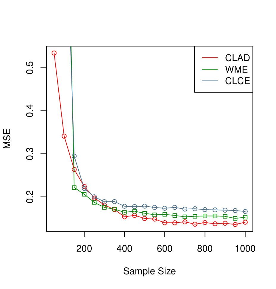
(a) $\hat{\beta}_{0}$

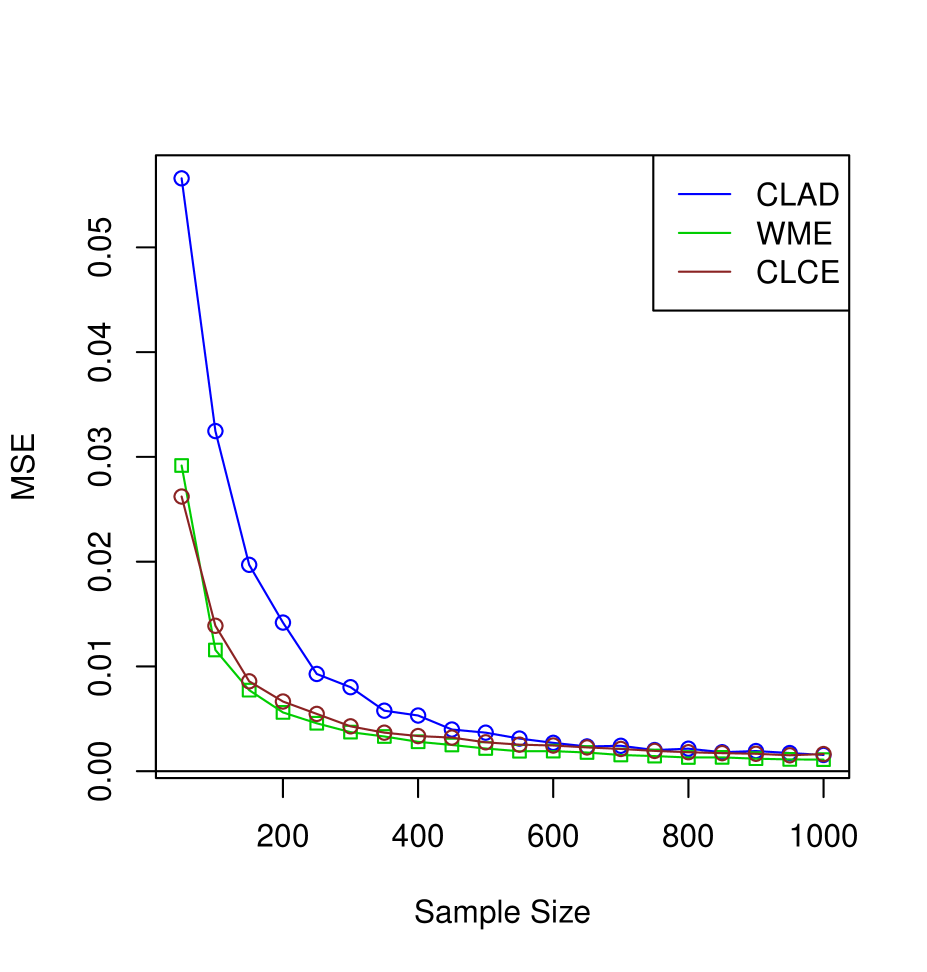
(b) $\hat{\beta}_{1}$

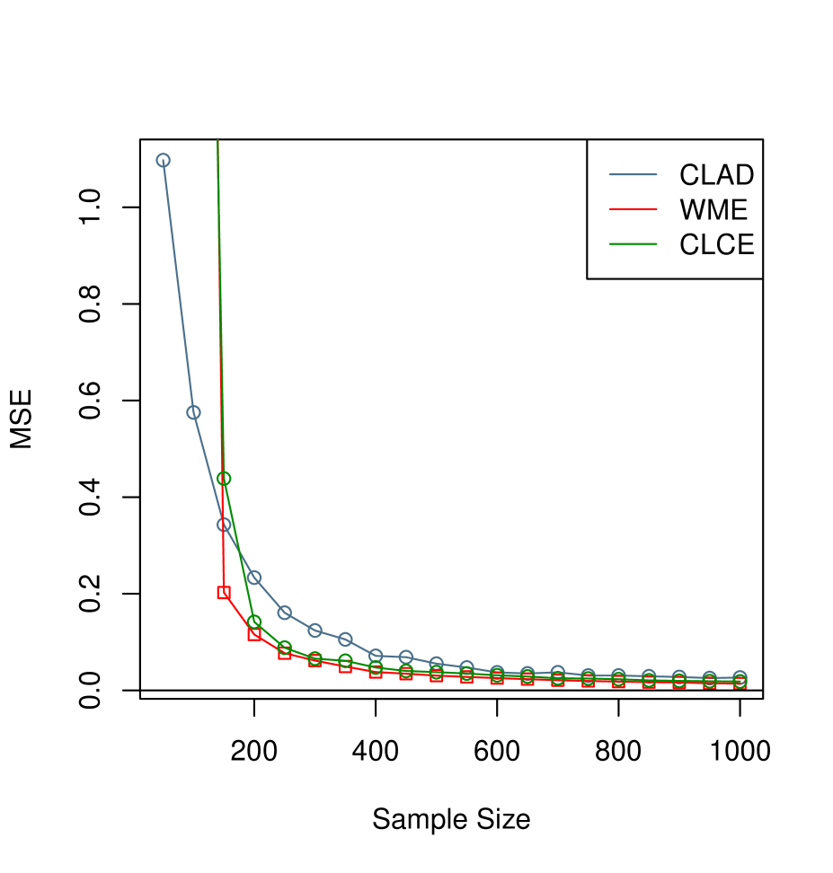
(c) $\hat{\beta}_{2}$

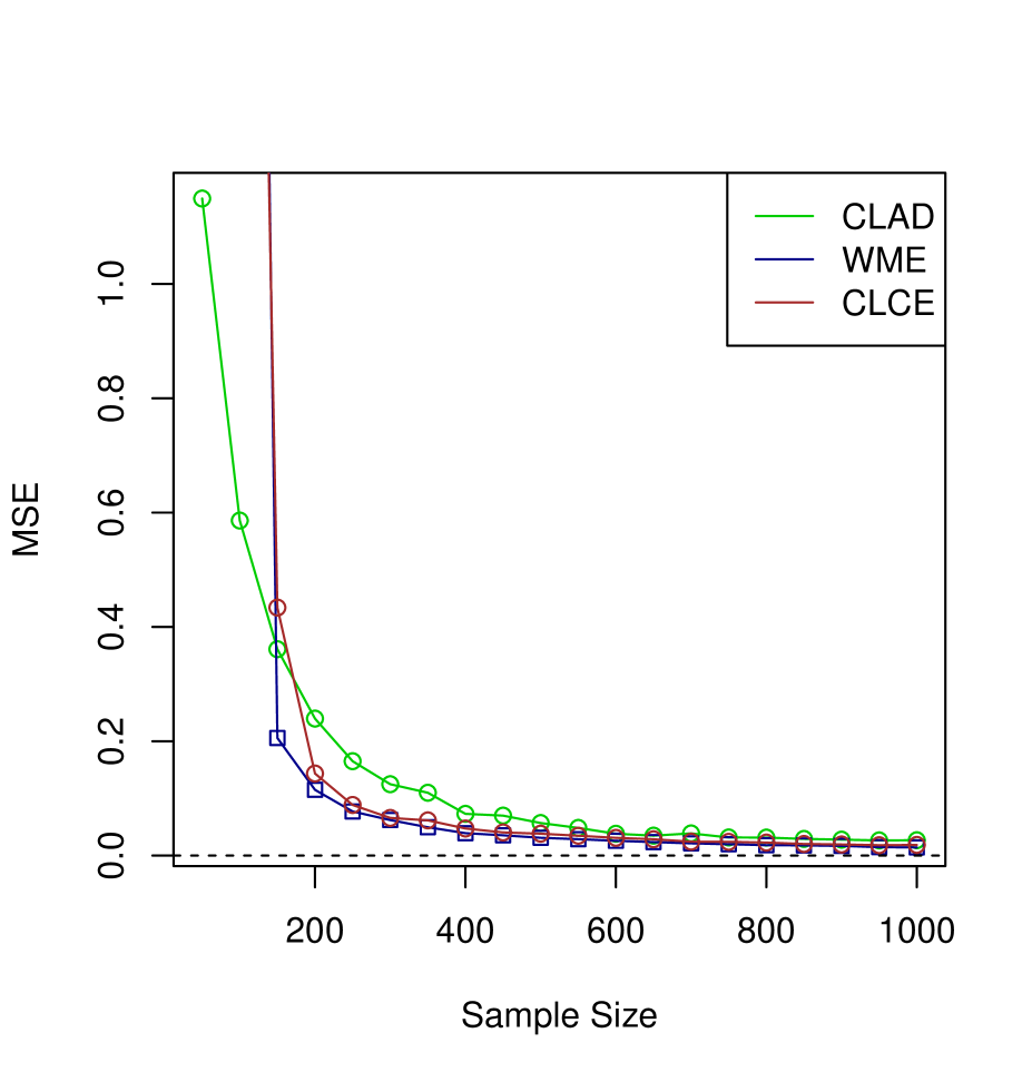
(d) $\hat{\rho}_{1}$

Figure 1: Empirical MSE for CLAD, WME and CLCE estimates of $\hat{\beta}_{0}$, $\hat{\beta}_{1}$, $\hat{\beta}_{3}$, and $\hat{\rho}_{1}$ when errors follow $N(0,1)$ for $n=50,100,150,\ldots,1000$

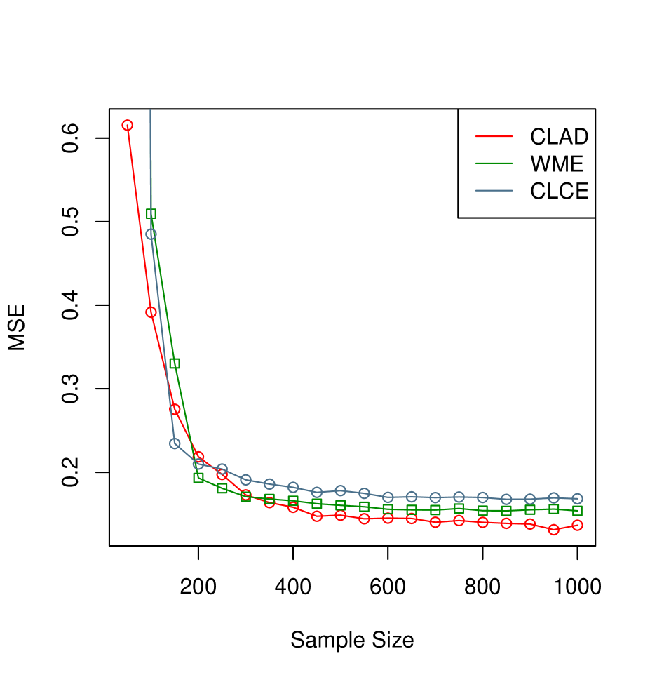
(a) $\hat{\beta}_{0}$

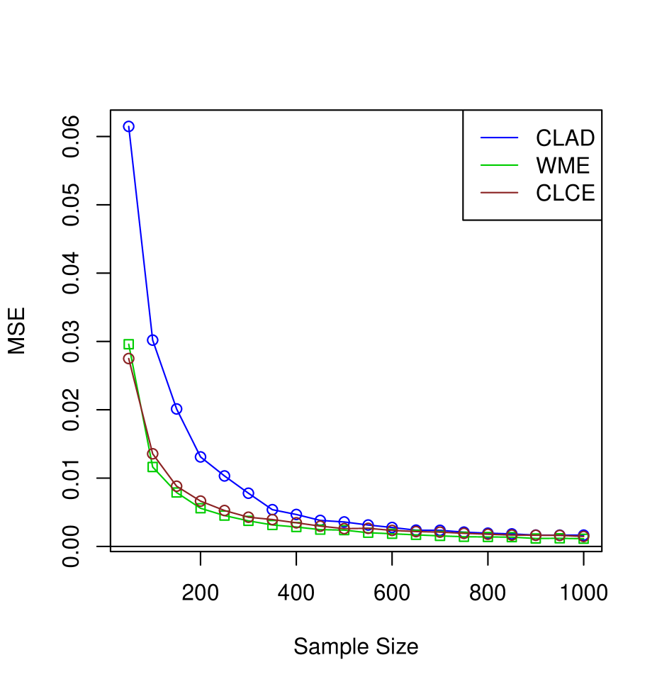
(b) $\hat{\beta}_{1}$

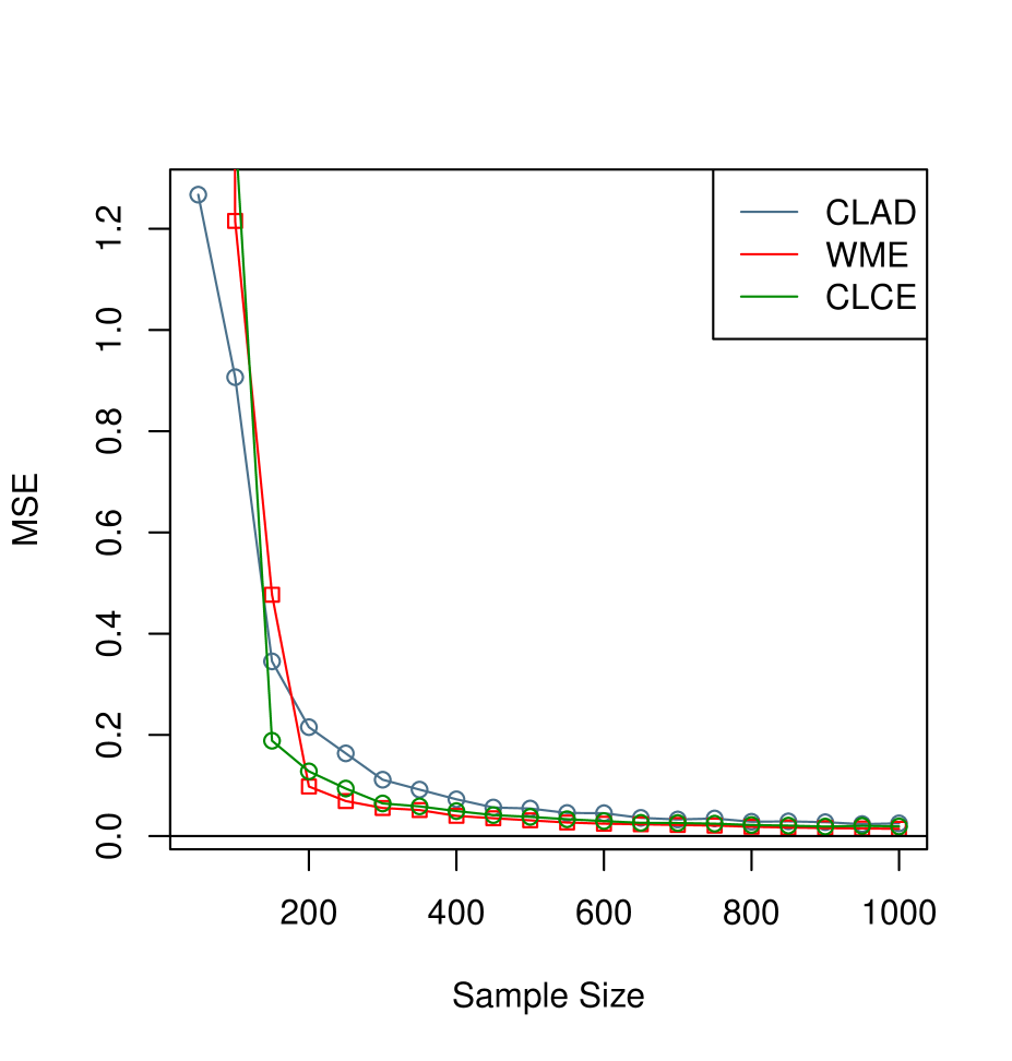
(c) $\hat{\beta}_{2}$

(d) $\hat{\rho}_{1}$

Figure 2: Empirical MSE for CLAD, WME and CLCE estimates of $\hat{\beta}_{0},$ $\hat{\beta}_{1}$,$\hat{\beta}_{3}$ and $\hat{\rho}_{1}$ when errors follow $DE(0,1)$ for $n=50,100,150,\ldots,1000$.

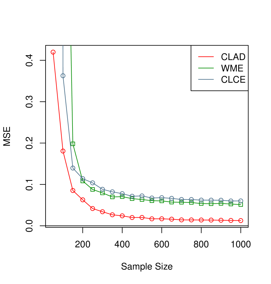
(a) $\hat{\beta}_{0}$

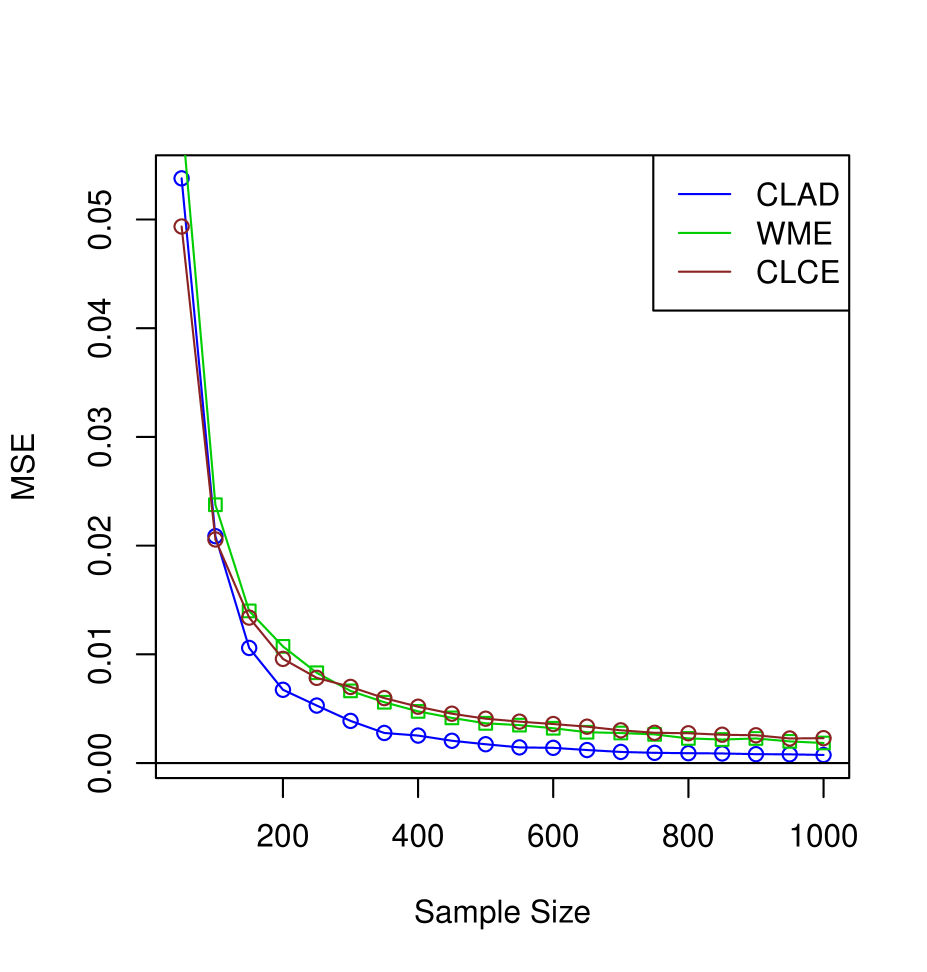
(b) $\hat{\beta}_{1}$

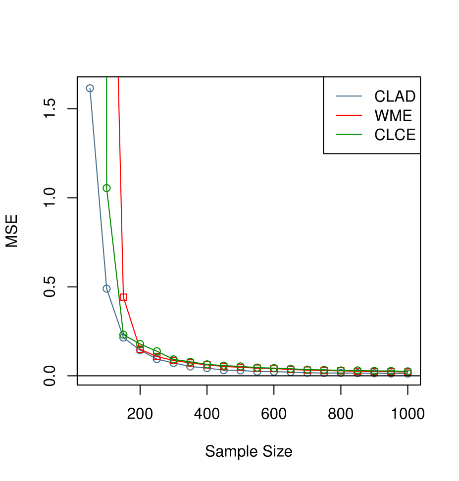
(c) $\hat{\beta}_{2}$

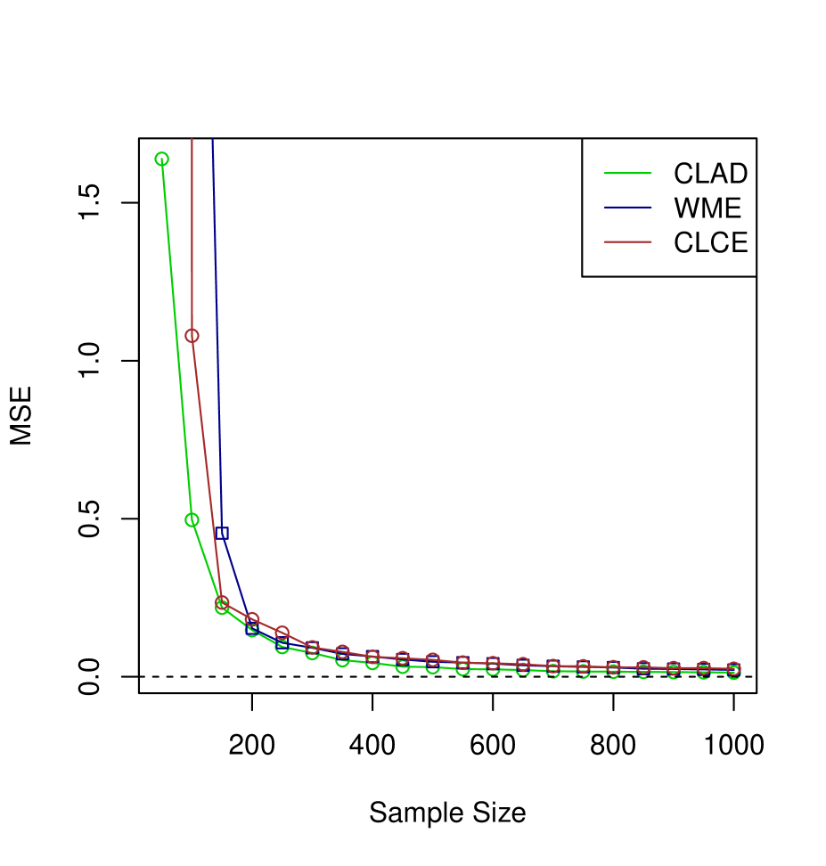
(d) $\hat{\rho}_{1}$

Figure 3: Empirical MSE for CLAD, WME and CLCE estimates of $\hat{\beta}_{0},$ $\hat{\beta}_{1}$,$\hat{\beta}_{3}$ and $\hat{\rho}_{1}$ when errors follow $t_{n}$ for $n=50,100,150,\ldots,1000.$

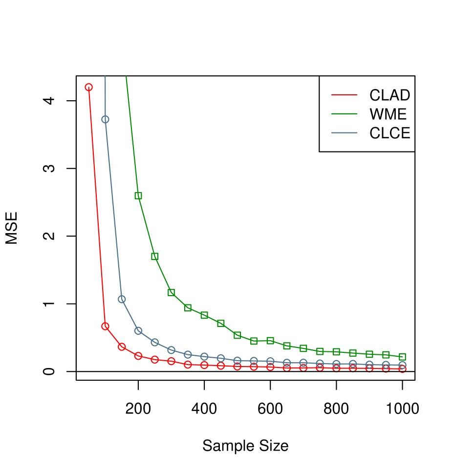
(a) $\hat{\beta}_{0}$

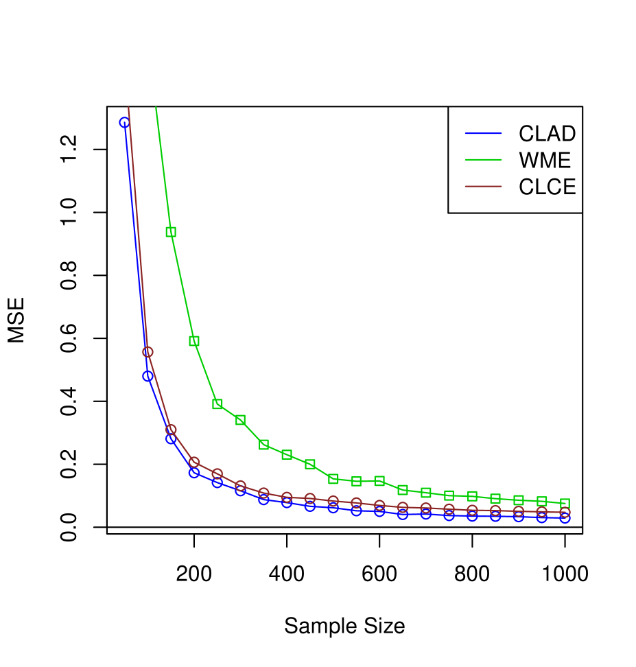
(b) $\hat{\beta}_{1}$

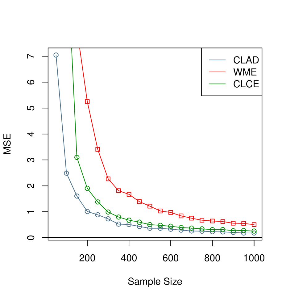
(c) $\hat{\beta}_{2}$

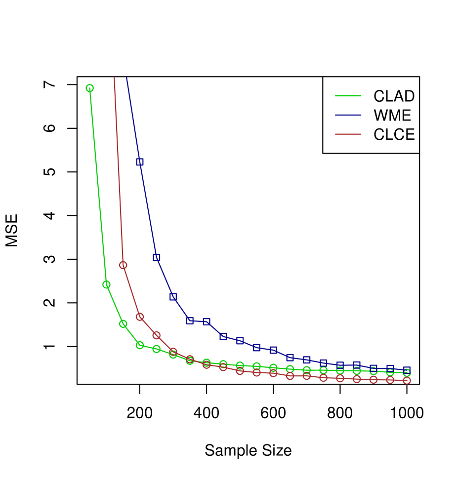
(d) $\hat{\rho}_{1}$

Figure 4: Empirical MSE for CLAD, WME and CLCE estimates of $\hat{\beta}_{0},$ $\hat{\beta}_{1}$,$\hat{\beta}_{3}$ and $\hat{\rho}_{1}$ when errors follow $N(0,\sigma_{X_{i}}^{2})$, where $\sigma_{X_{i}}^{2}=(\boldsymbol{X}^{T}_{i}\boldsymbol{\beta})^{2}$ for $n=50,100,150,\ldots,1000.$

It is evident from Figures 1, 2 and 3 that in the presence of endogenous variables, the estimators of the parameters associated with the model (2.8) are consistent, as it is theoretically established in Theorem 3.1. Next, Figure 4 represents the comparison of the MSE of these estimators in the case of heteroskedasticity, and it is observed that the MSEs of WME and CLCE estimators are higher than that of CLAD for small sample sizes, but as the sample size increases, eventually the MSEs decrease. So, it is evident that in the case of heteroskedasticity, the MSEs are approaching zero as the sample size increases. Hence, these estimators are performing well in the case of all error distributions, including non-normal distributions, considered here.

Table 3 represents the empirical bias and empirical MSE of symmetrically censored least squares (SCLS) when the support of the error distribution is bounded. We perform a simulation study based on truncated normal distribution, truncated Laplace distribution, truncated $t$-distribution, and $N(0,\sigma_{X_{i}}^{2})$, where $\sigma_{X_{i}}^{2}=(\boldsymbol{X}^{T}_{i}\boldsymbol{\beta})^{2}$ as error distribution. For a small sample size, the values reported in Table 3 indicate that the MSEs of $\beta_{2}$ and $\rho_{1}$ are higher as compared to that of $\beta_{1}$ and $\beta_{0}$.

Table 3: Empirical bias and MSE of $\hat{\beta_{0}},$ $\hat{\beta_{1}},$ $\hat{\beta_{2}}$ and $\hat{\rho_{1}}$ with $n=50,100,500,1000.$

Estimators	$\boldsymbol{\beta}$	Error-distribution
		$N(0,1)$			$DE(0,1)$			$t_{n}$			$N(0,\sigma_{X_{i}}^{2})$, $\sigma_{X_{i}}^{2}=(\boldsymbol{X}^{T}_{i}\boldsymbol{\beta})^{2}$
		Bias	MSE	C.P	Bias	MSE	C.P	Bias	MSE	C.P	Bias	MSE	C.P
		$n=50$
	$\beta_{0}$	0.0436	0.9645		0.0512	2.0848		0.0398	3.7091		0.0220	2.5667
SCLS	$\beta_{1}$	0.0040	0.0127	26$\%$	-0.0002	0.0102	30$\%$	0.0051	0.0121	28$\%$	0.0119	0.0381	38$\%$
	$\beta_{2}$	-0.1036	3.4037		-0.1494	9.3995		-0.1429	10.237		-0.0435	14.448
	$\rho_{1}$	0.1109	3.4103		0.1499	9.3870		0.1459	10.236		0.0645	14.404
		$n=100$
	$\beta_{0}$	-0.0024	8.7150		0.1545	6.3232		0.1256	2.4670		0.0654	2.2007
SCLS	$\beta_{1}$	0.0018	0.0057	25$\%$	0.0018	0.0051	22$\%$	0.0004	0.0054	25$\%$	0.0084	0.0181	33$\%$
	$\beta_{2}$	-0.0604	1.8580		0.0102	4.7568		-0.0527	1.8049		-0.0845	1.0643
	$\rho_{1}$	0.0620	1.8618		-0.0050	4.7580		0.0514	1.8140		0.0932	1.0663
		$n=500$
	$\beta_{0}$	0.0052	0.0077		0.0034	0.0067		0.0055	0.0076		0.0020	0.0165
SCLS	$\beta_{1}$	-0.0003	0.0011	22$\%$	0.0018	0.0009	29$\%$	0.0009	0.0011	24.2$\%$	0.0032	0.0035	28.2$\%$
	$\beta_{2}$	-0.0113	0.0200		-0.0114	0.0188		-0.0097	0.0201		-0.0096	0.0426
	$\rho_{1}$	0.0119	0.0205		0.0117	0.0192		0.0093	0.0203		0.0115	0.0438
		$n=1000$
	$\beta_{0}$	0.0045	0.0035		0.0020	0.0033		0.0020	0.0034		0.0035	0.0078
SCLS	$\beta_{1}$	0.0001	0.0005	25.7$\%$	0.0004	0.0005	28.4$\%$	-0.0005	0.0005	29$\%$	0.0007	0.0017	27.6$\%$
	$\beta_{2}$	-0.0080	0.0090		-0.0053	0.0082		-0.0046	0.0087		-0.0092	0.0194
	$\rho_{1}$	0.0078	0.0092		0.0060	0.0080		0.0058	0.0090		0.0102	0.0199

5 Real Data Study

To illustrate the applicability of the proposed estimators over other estimators, we consider a well-known data set, Mroz data. This Mroz (1987) data set is available in the Wooldridge R package (see https://rdrr.io/rforge/Ecdat/man/Mroz.html), which pertains to U.S. women’s labor force participation. The data set contains observations on 753 individuals. The dependent variable is the total number of hours worked per week. In the data, 325 of the 753 women worked 0 hours; therefore, the dependent variable is left-censored at zero. Hence, the censoring probability is approximately 0.43. For this data set, the explanatory variables are years of education (educ), years of experience (exper) and its square (expersq), age of the wife (age), number of children under six years old (kidslt6), number of children equal to or greater than six years old (kidsge6), and non-wife household income (nwifeinc). We consider nwifeinc to be an endogenous variable since it may be correlated to unobserved household preferences regarding the wife’s labor force participation. We add the husband’s years of schooling (huseduc) as an instrument because it can influence both his income and the now-wife’s household income, but it should not influence the wife’s decision to engage in the labor force.

Table 4: Parameter estimates of Tobit model

Variables	CLAD	WME	CLCE
age	-0.4580	0.5077	-0.2991
educ	0.3550	0.8450	0.1719
exper	1.1123	1.5373	0.9289
expersq	-0.4014	-1.9696	-0.3233
kidslt6	-0.7913	0.0358	0.0724
kidsge6	0.2221	0.0978	-0.1578
nwifeinc	0.1249	-2.5682	-1.2380
residual	-0.3397	2.6877	0.8040

Table 5: Bootstrap MSE of CLAD, WME, and CLCE Estimator for $B=500,1000,1500$.

Parameters	BMSE
	CLAD			WME			CLCE
	$B=500$	$B=1000$	$B=1500$	$B=500$	$B=1000$	$B=1500$	$B=500$	$B=1000$	$B=1500$
age	0.7118	0.7011	0.6985	0.3518	0.3604	0.3645	0.5177	0.4941	0.4618
educ	0.5898	0.5855	0.6129	0.4844	0.4811	0.4676	0.6843	0.7085	0.6672
exper	0.4927	0.5439	0.4890	2.8544	3.1788	3.1627	1.6108	1.6805	1.5337
expersq	1.8319	1.7724	1.8819	3.8145	4.3454	4.2618	1.5171	1.6423	1.4472
kidslt6	2.9191	2.8311	2.9829	0.1231	0.1228	0.1213	0.1535	0.1541	0.1613
kidsge6	0.7251	0.7112	0.7530	0.0904	0.1065	0.1066	0.2150	0.1889	0.1798
nwifeinc	0.8463	0.8253	0.8776	4.4537	4.5254	4.1562	2.9621	2.9260	2.9958
residual	1.6876	1.6326	1.7354	4.9339	5.0020	4.6065	3.9345	3.8406	3.8480

To validate the theoretical result on the real data set, estimates and bootstrap mean square error (MSE) are computed in this part. Following are the steps to find the bootstrap mean square error (BMSE) of parameters in the Tobit model using the control function approach:

• First, obtain the residual from the linear regression model by regressing the endogenous variable (nwifeinc) on the instrumental variable (husedu). To address endogeneity and create a control function, the residual obtained from the previous step is incorporated into the Tobit model.

• Estimate the Tobit model parameters, which contain the explanatory variables and the control function, using the original data set. Here, $\hat{\theta}_{1},\ldots,\hat{\theta}_{p},$ represents the $p$ true parameter values.

• Using basic random sampling with replacement, generate $B$ bootstrap samples $\{s^{*}_{1},\ldots,s^{*}_{B}\}$ from the original data set to create a new data set of the same size as the original data set.

• Estimate the parameters of the Tobit model for each bootstrap sample, which is denoted as $\{\hat{\boldsymbol{\theta}}^{*}_{1},\hat{\boldsymbol{\theta}}^{*}_{2},\ldots,\hat{\boldsymbol{\theta}}^{*}_{B}\}.$

• Compute the bootstrap mean square error (BMSE) between the bootstrap estimates and the true parameter value for each bootstrap sample.

• Use the following formula to find the average BMSE for each parameter over all bootstrap samples:

  $$BMSE=\frac{1}{B}\sum_{b=1}^{B}\left(\hat{\theta}_{ib}-\hat{\theta}_{i}\right)^{2}$$

  where $\hat{\theta}_{ib}$ is the $ith$ element of $\hat{\boldsymbol{\theta}}^{*}_{b}$, $b=1,\ldots,B$ and $i=1,\ldots,p.$

Table 4 contains the results of parameter estimates for the Tobit model. In the table, the second column gives the CLAD parameter estimates (see, (2.12)), the third column gives the WME estimates (see, (2.13)), and the last column gives the CLCE estimates (see, (2.14)). The interpretation of these estimates shows interesting patterns in the relationship between various factors and the working hours of married women.

Regarding CLAD and CLCE, the age coefficient is negative, demonstrating that married women work fewer hours as they get older. Nevertheless, WME has a positive coefficient, representing that working hours increase with age. Across all three cases (CLAD, WME, and CLCE), a positive coefficient for education (educ) and experience (exper) indicates that married women who hold higher levels of education also work for a longer period of time. Furthermore, the coefficient for the squared term of experience (expersq) is negative in all three cases. This implies that, where more working hours are initially associated with more experience, this effect wanes as experience levels increase. There is evidence that married women with small children work less hours; this is indicated by the variable (kidslt6) having a negative coefficient.

In the overall context, working hours for CLAD and CLCE are positively impacted by kidsge6, nwifeinc, and the residual term, but negatively impacted by age, education, experience, and kidslt6. In the case of WME, working hours are positively influenced by age, education, experience, and kidslt6, but adversely affected by kidsge6 and nwifeinc. The residual term also has a positive impact. Table 5 represents the BMSE of parameter estimates. When the number of bootstrap samples ($B$) increases, CLAD shows consistent improvement in BMSE across all parameters. Overall, it does quite well. The performance of WME is mixed. As the bootstrap sample size increases, it shows improvement for certain parameters (e.g., kidslt6) but increases BMSE for other parameters (e.g., exper, expersq). In contrast, CLCE consistently performs well in BMSE as $B$ increases, outperforming WME and CLAD overall.

6 Conclusion

In this study, we have proposed and studied the M-estimation for the Tobit model with an endogenous regressor. By incorporating the control function technique using instrumental variables, we address endogeneity issues in the Tobit model. In the presence of left censoring, our proposed method allows the exploration of M-estimation with a control function technique to accommodate a general non-convex, non-differentiable, and non-monotone loss function. Our method is adaptable and suitable for a wide range of applications because the loss function that is taken into account covers well-known instances such as Huber, least absolute, and log-cosh.

Through rigorous theoretical analysis, the strong consistency and asymptotic normality of the M-estimator under some regularity conditions are derived. Additionally, a consistent estimation procedure for the estimation of the covariance matrix of the asymptotic distribution of the proposed M-estimators is developed. The finite sample performance of three different estimators- CLAD, WME, and CLCE- of the parameters in the Tobit model through an extensive simulation study with a large sample size. The analyses included both heteroskedastic and homoskedastic error distributions. The results of the simulation study indicate that all estimators perform well under various different conditions. The effectiveness of the suggested methodology, in particular the CLCE estimator corresponding to the log-cosh loss function, was demonstrated by the data. It is noteworthy that the proposed estimator CLCE consistently outperforms over CLAD and WME with respect to MSE.

To further validate the proposed methodology, we conducted a real data study by representing the bootstrap MSE estimates of parameters. The empirical results reinforced the improved performance of the estimators, affirming their robustness in practical applications. This research provides significant insight into the statistical modeling of endogenous regressors in censored data. It is possible to extend this concept in the future to identify rank-based estimators when endogenous regressors are present. In this investigation, a continuous endogenous regressor has been taken into consideration. A similar method can also be used to extend this concept to binary endogenous variables.

Acknowledgement : Subhra Sankar Dhar gratefully acknowledges his core research grant CRG/2022/001489, Government of India.

7 Appendix

$\boldsymbol{B.1.}$ Consistency

In this section, we present the proof of the Theorem 3.1 stated in Section 3 to show strong consistency of the M-estimator for the model (2.8). It is similar to those used by [45] to demonstrate the strong consistency of the LAD estimator for the standard Tobit model and [42] to demonstrate the weak consistency of the LAD estimator for the nonlinear regression model. The following lemmas of [55] are employed in the following proof:

Lemma 7.1 (Lemma 2.3 of [55]).

Let $\{y_{i}\}$ be a sequence of independent random variables that takes value in $(\Omega,\mathcal{F})$,$\mathcal{F}$ is a $\sigma$-field. Let $\rho\colon(\Omega,\mathcal{B})\to\mathbb{R}$, where $\mathcal{B}\in\mathbb{R}^{m}$ is compact. Assume that

1. For each $\boldsymbol{\beta}$ in $\mathcal{B},$ $\rho(\omega,\boldsymbol{\beta})$ is $\mathcal{F}$-measurable.

2. $\rho(y_{i},\boldsymbol{\beta})$ is continuous on $\mathcal{B}$, uniformly in i, a.s.

3. There exists a measurable $m_{i}\colon\Omega\to\mathbb{R}$ for which $|\rho(\omega,\boldsymbol{\beta})|<m_{i}(\omega),\hskip 2.84544pt\forall\boldsymbol{\beta}\in\mathcal{B},$ and for all i, $E\left[m_{i}(y_{i})\right]^{1+\delta^{*}}\leq M<\infty,$ and some $\delta^{*}>0.$ Then

   1. $E\left[\rho(y_{i},\boldsymbol{\beta})\right]$ is continuous on $\mathcal{B}$, uniformly in i.

   2. $\underset{\boldsymbol{\beta}\;\in\;\mathcal{B}}{\text{sup}}\;\left|\frac{1}{n}\sum\limits_{i=1}^{n}\rho(y_{i},\boldsymbol{\beta})-\overline{S}_{n}(\boldsymbol{\beta})\right|\overset{a.s}{\to}0,$ where $\overline{S}_{n}(\boldsymbol{\beta})=\frac{1}{n}\sum\limits_{i=1}^{n}E\left[\rho(y_{i},\boldsymbol{\beta})\right].$

Lemma 7.2 (Lemma 2.2 of [55]).

Let $S_{n}(\omega,\boldsymbol{\beta})$ be a measurable function on a measurable space $(\Omega,\mathcal{F})$ and a continuous function of $\boldsymbol{\beta}$ on a compact set $\mathcal{B}$ for each $\omega$ in $\Omega.$ Then there exists a measurable function $\hat{\beta}_{n}(\omega)$ such that

$$S_{n}\left[\omega,\hat{\boldsymbol{\beta}}_{n}(\omega)\right]=\underset{\boldsymbol{\beta}\;\in\;\mathcal{B}}{\text{inf}}S_{n}\left(\omega,\boldsymbol{\beta}\right)$$

for all $\omega$ in $\Omega.$ if $\left|S_{n}(\omega,\boldsymbol{\beta})-\overline{S}_{n}(\boldsymbol{\beta})\right|\overset{a.s}{\to}0.$ uniformly for all $\boldsymbol{\beta}$ in $\mathcal{B}$ and if $\overline{S}_{n}(\boldsymbol{\beta})$ has a minimum at $\boldsymbol{\beta}_{0}$ which is identifiably unique(i.e., for any $\epsilon^{*}>0$,

$$\underset{n\geq n_{0}}{\text{inf}}\underset{\boldsymbol{\beta}}{\text{min}}\left\{\overline{S}_{n}(\boldsymbol{\beta})-\overline{S}_{n}(\boldsymbol{\beta}_{0})\colon\boldsymbol{\beta}\in\mathcal{B},\|\boldsymbol{\beta}-\boldsymbol{\beta}_{0}\|>\epsilon^{*}\right\}>0$$

for some positive integer $n_{0}$), then $\hat{\boldsymbol{\beta}}_{n}$ converges to $\boldsymbol{\beta}_{0}$ almost surely $(\omega).$

Proof of Theorem 3.1..

Suppose

$$\xi_{i}^{*}=y_{i}-max\{0,\boldsymbol{X}_{i}^{T}\boldsymbol{\beta}_{0}\},$$ (7.1)

and define

$$h_{i}=h_{i}(\boldsymbol{\beta},\boldsymbol{\beta}_{0})=max\{0,\boldsymbol{X}_{i}^{T}\boldsymbol{\beta}\}-max\{0,\boldsymbol{X}_{i}^{T}\boldsymbol{\beta}_{0}\},$$ (7.2)

where $\boldsymbol{\delta}^{*}=\boldsymbol{\beta}-\boldsymbol{\beta}_{0}$, First, note that minimizing $Q_{n}(\boldsymbol{\beta})$ is equivalent to minimizing the normalized function

$$S_{n}(\boldsymbol{\beta})=Q_{n}(\boldsymbol{\beta})-Q_{n}(\boldsymbol{\beta}_{0}),$$ (7.3)

which can be written as

$$S_{n}(\boldsymbol{\beta})=\frac{1}{n}\sum\limits_{i=1}^{n}\rho\left(y_{i}-max\{0,\boldsymbol{X}_{i}^{T}\boldsymbol{\beta}\}\right)-\frac{1}{n}\sum\limits_{i=1}^{n}\rho\left(y_{i}-max\{0,\boldsymbol{X}_{i}^{T}\boldsymbol{\beta}_{0}\}\right)$$ (7.4)

Since $Q_{n}(\boldsymbol{\beta}_{0})$ is independent of $\boldsymbol{\beta}$, normalization has no impact on the sequence of minimizing values $\{\hat{\beta}_{n}\}.$ Now we will show that $S_{n}(\boldsymbol{\beta})$ will satisfy the conditions of the lemma (7.1). Then, using (7.4), we obtain

$$\begin{split}S_{n}(\boldsymbol{\beta})&=\frac{1}{n}\sum\limits_{i=1}^{n}\rho\left(\xi_{i}^{*}-h_{i}\right)-\frac{1}{n}\sum\limits_{i=1}^{n}\rho\left(\xi_{i}^{*}\right)\\ &=\frac{1}{n}\sum\limits_{i=1}^{n}\left[\rho(\xi_{i}^{*}-h_{i})-\rho(\xi_{i}^{*})\right]\\ &\leq\frac{1}{n}\sum\limits_{i=1}^{n}\left|\rho(\xi_{i}^{*}-h_{i})-\rho(\xi_{i}^{*})\right|\\ &\leq\frac{k}{n}\sum\limits_{i=1}^{n}\left|\xi_{i}^{*}-h_{i}-\xi_{i}^{*}\right|=\frac{k}{n}\sum\limits_{i=1}^{n}\left|h_{i}\right|\end{split}$$ (7.5)

$$\begin{split}\text{and}\;|h_{i}|=|h_{i}(\boldsymbol{\beta},\boldsymbol{\beta}_{0})|&=\left|max\{0,\boldsymbol{X}_{i}^{T}\boldsymbol{\beta}\}-max\{0,\boldsymbol{X}_{i}^{T}\boldsymbol{\beta}_{0}\}\right|\\ &=\left|\frac{1}{2}\left[\boldsymbol{X}_{i}^{T}\boldsymbol{\beta}+|\boldsymbol{X}_{i}^{T}\boldsymbol{\beta}|\right]-\frac{1}{2}\left[\boldsymbol{X}_{i}^{T}\boldsymbol{\beta}_{0}+|\boldsymbol{X}_{i}^{T}\boldsymbol{\beta}_{0}|\right]\right|\\ &=\left|\frac{1}{2}\left[\boldsymbol{X}_{i}^{T}(\boldsymbol{\beta}-\boldsymbol{\beta}_{0})\right]+\frac{1}{2}\left[|\boldsymbol{X}_{i}^{T}\boldsymbol{\beta}|-|\boldsymbol{X}_{i}^{T}\boldsymbol{\beta}_{0}|\right]\right|\\ &\leq\frac{1}{2}\left|\boldsymbol{X}_{i}^{T}\left(\boldsymbol{\beta}-\boldsymbol{\beta}_{0}\right)\right|+\frac{1}{2}\left|\boldsymbol{X}_{i}^{T}\left(\boldsymbol{\beta}-\boldsymbol{\beta}_{0}\right)\right|=\left|\boldsymbol{X}_{i}^{T}\left(\boldsymbol{\beta}-\boldsymbol{\beta}_{0}\right)\right|\\ &\leq\|\boldsymbol{X}_{i}\|\;\|\boldsymbol{\beta}-\boldsymbol{\beta}_{0}\|\\ &\leq\|\boldsymbol{X}_{i}\|\left(\|\boldsymbol{\beta}\|+\|\boldsymbol{\beta}_{0}\|\right)=\mathcal{O}(\|\boldsymbol{X}_{i}\|).\\ \end{split}$$ (7.6)

Because summand ($|h_{i}|$) in ((7.5)) is bounded (in magnitude) by $\|\boldsymbol{X}_{i}\|\left(\|\boldsymbol{\beta}\|+\|\boldsymbol{\beta}_{0}\|\right)$, which is $\mathcal{O}(\|\boldsymbol{X}_{i}\|)$ due to the compactness of $\mathcal{B}$. Assumptions $\boldsymbol{A.2}$ and $\boldsymbol{A.3}$, as well as Lemma 7.1, lead to

$$\underset{n\to\infty}{lim}\left|S_{n}\left(\boldsymbol{\beta}\right)-E\left[S_{n}\left(\boldsymbol{\beta}\right)\right]\right|=0\hskip 5.69046pta.s.,$$ (7.7)

uniformly in $\boldsymbol{\beta}$. Since $E\left[S_{n}(\boldsymbol{\beta}_{0})\right]=0$, according to Lemma 7.2, $\hat{\boldsymbol{\beta}}_{n}$ is strongly consistent if for every $\epsilon^{*}>0,$ $E\left[S_{n}\left(\boldsymbol{\beta}\right)\right]$ is bounded away from 0, uniformly in $\boldsymbol{\beta}$ for $\|\boldsymbol{\beta}-\boldsymbol{\beta}_{0}\|\geq\epsilon^{*}$ and for all sufficiently large $n$. Since $E\left[Q_{n}\left(\boldsymbol{\beta}\right)\right]$ is not convex in $\boldsymbol{\beta}$. Therefore, to demonstrate that $E\left[Q_{n}\left(\boldsymbol{\beta}\right)-Q_{n}\left(\boldsymbol{\beta}_{0}\right)\right]$ has unique minima whenever $\boldsymbol{\beta}$ near $\boldsymbol{\beta}_{0},$ the conditional expectation of $S_{n}(\boldsymbol{\beta})$ can be expressed as

$$E\left[S_{n}\left(\boldsymbol{\beta}\right)|\boldsymbol{X}_{1},\ldots,\boldsymbol{X}_{n}\right]=E\left[Q_{n}\left(\boldsymbol{\beta}\right)|\boldsymbol{X}_{1},\ldots,\boldsymbol{X}_{n}\right]-E\left[Q_{n}\left(\boldsymbol{\beta}_{0}\right)|\boldsymbol{X}_{1},\ldots,\boldsymbol{X}_{n}\right].$$ (7.8)

We determine $E\left[Q_{n}\left(\boldsymbol{\beta}\right)\right]$ and $E\left[Q_{n}\left(\boldsymbol{\beta}_{0}\right)\right]$ individually, then we subtract it to demonstrate that the individual term is positive.

$$\begin{split}E\left[Q_{n}\left(\boldsymbol{\beta}\right)|\boldsymbol{X}_{1},\ldots,\boldsymbol{X}_{n}\right]&=\frac{1}{n}\sum\limits_{i=1}^{n}\mathds{1}\left(\boldsymbol{X}^{T}_{i}\boldsymbol{\beta}>0\right)E_{\xi|\boldsymbol{X}}\left[\rho\left(y_{i}-\boldsymbol{X}^{T}_{i}\boldsymbol{\beta}\right)\right]+\mathds{1}\left(\boldsymbol{X}^{T}_{i}\boldsymbol{\beta}<0\right)E_{\xi|\boldsymbol{X}}\left[\rho\left(y_{i}\right)\right]\\ &=\frac{1}{n}\sum\limits_{i=1}^{n}\mathds{1}\left(\boldsymbol{X}^{T}_{i}\boldsymbol{\beta}>0\right)\left\{\mathds{1}\left(\boldsymbol{X}^{T}_{i}\boldsymbol{\beta}_{0}>0\right)E_{\xi|\boldsymbol{X}}\left[\rho\left(y_{i}-\boldsymbol{X}^{T}_{i}\boldsymbol{\beta}\right)\right]\right\}\\ &+\frac{1}{n}\sum\limits_{i=1}^{n}\mathds{1}\left(\boldsymbol{X}^{T}_{i}\boldsymbol{\beta}>0\right)\left\{\mathds{1}\left(\boldsymbol{X}^{T}_{i}\boldsymbol{\beta}_{0}<0\right)E_{\xi|\boldsymbol{X}}\left[\rho\left(y_{i}-\boldsymbol{X}^{T}_{i}\boldsymbol{\beta}\right)\right]\right\}\\ &+\frac{1}{n}\sum\limits_{i=1}^{n}\mathds{1}\left(\boldsymbol{X}^{T}_{i}\boldsymbol{\beta}<0\right)\bigr{\{}\mathds{1}\left(\boldsymbol{X}^{T}_{i}\boldsymbol{\beta}_{0}>0\right)E_{\xi|\boldsymbol{X}}\left[\rho\left(y_{i}\right)\right]\\ &+\mathds{1}\left(\boldsymbol{X}^{T}_{i}\boldsymbol{\beta}_{0}<0\right)E_{\xi|\boldsymbol{X}}\left[\rho\left(y_{i}\right)\right]\bigr{\}}.\end{split}$$ (7.9)

Similarly,

$$\begin{split}E\left[Q_{n}(\boldsymbol{\beta}_{0})|\boldsymbol{X}_{1},\ldots,\boldsymbol{X}_{n}\right]&=\frac{1}{n}\sum\limits_{i=1}^{n}\bigr{\{}\mathds{1}\left(\boldsymbol{X}^{T}_{i}\boldsymbol{\beta}_{0}>0\right)E_{\xi|\boldsymbol{X}}\left[\rho\left(y_{i}-\boldsymbol{X}^{T}_{i}\boldsymbol{\beta}_{0}\right)\right]\\ &+\mathds{1}\left(\boldsymbol{X}^{T}_{i}\boldsymbol{\beta}_{0}<0\right)E_{\xi|\boldsymbol{X}}\left[\rho\left(y_{i}\right)\right]\bigr{\}}\\ &=\frac{1}{n}\sum\limits_{i=1}^{n}\mathds{1}\left(\boldsymbol{X}^{T}_{i}\boldsymbol{\beta}_{0}>0\right)\left\{\mathds{1}\left(\boldsymbol{X}^{T}_{i}\boldsymbol{\beta}>0\right)E_{\xi|\boldsymbol{X}}\left[\rho\left(y_{i}-\boldsymbol{X}^{T}_{i}\boldsymbol{\beta}_{0}\right)\right]\right\}\\ &+\frac{1}{n}\sum\limits_{i=1}^{n}\mathds{1}\left(\boldsymbol{X}^{T}_{i}\boldsymbol{\beta}_{0}>0\right)\left\{\mathds{1}\left(\boldsymbol{X}^{T}_{i}\boldsymbol{\beta}<0\right)E_{\xi|\boldsymbol{X}}\left[\rho\left(y_{i}-\boldsymbol{X}^{T}_{i}\boldsymbol{\beta}_{0}\right)\right]\right\}\\ &+\frac{1}{n}\sum\limits_{i=1}^{n}\mathds{1}\left(\boldsymbol{X}^{T}_{i}\boldsymbol{\beta}_{0}<0\right)\bigr{\{}\mathds{1}\left(\boldsymbol{X}^{T}_{i}\boldsymbol{\beta}>0\right)E_{\xi|\boldsymbol{X}}\left[\rho\left(y_{i}\right)\right]\\ &+\mathds{1}\left(\boldsymbol{X}^{T}_{i}\boldsymbol{\beta}<0\right)E_{\xi|\boldsymbol{X}}\left[\rho\left(y_{i}\right)\right]\bigr{\}}.\end{split}$$ (7.10)

Subtract the (7.10) from the (7.9), and we have

$$E\left[Q_{n}\left(\boldsymbol{\beta}\right)-Q_{n}\left(\boldsymbol{\beta}_{0}\right)|\boldsymbol{X}_{1},\ldots,\boldsymbol{X}_{n}\right]=E\left[S_{n}\left(\boldsymbol{\beta}\right)|\boldsymbol{X}_{1},\ldots,\boldsymbol{X}_{n}\right]$$

$$\begin{split}&=\frac{1}{n}\sum\limits_{i=1}^{n}\left\{\mathds{1}\left(\boldsymbol{X}^{T}_{i}\boldsymbol{\beta}>0\right)\mathds{1}\left(\boldsymbol{X}^{T}_{i}\boldsymbol{\beta}_{0}>0\right)\right\}E_{\xi|\boldsymbol{X}}\left[\rho\left(y_{i}-\boldsymbol{X}^{T}_{i}\boldsymbol{\beta}\right)-\rho\left(y_{i}-\boldsymbol{X}^{T}_{i}\boldsymbol{\beta}_{0}\right)\right]\\ &+\frac{1}{n}\sum\limits_{i=1}^{n}\left\{\mathds{1}\left(\boldsymbol{X}^{T}_{i}\boldsymbol{\beta}>0\right)\mathds{1}\left(\boldsymbol{X}^{T}_{i}\boldsymbol{\beta}_{0}<0\right)\right\}E_{\xi|\boldsymbol{X}}\left[\rho\left(y_{i}-\boldsymbol{X}^{T}_{i}\boldsymbol{\beta}\right)-\rho\left(y_{i}\right)\right]\\ &+\frac{1}{n}\sum\limits_{i=1}^{n}\left\{\mathds{1}\left(\boldsymbol{X}^{T}_{i}\boldsymbol{\beta}<0\right)\mathds{1}\left(\boldsymbol{X}^{T}_{i}\boldsymbol{\beta}_{0}>0\right)\right\}E_{\xi|\boldsymbol{X}}\left[\rho\left(y_{i}\right)-\rho\left(y_{i}-\boldsymbol{X}^{T}_{i}\boldsymbol{\beta}_{0}\right)\right].\\ \end{split}$$ (7.11)

Since all terms in this expression are positive, using the assumption $\boldsymbol{A.5}$, there exists $k_{1}>0$ such that we have the following:

$$\begin{split}E\left[S_{n}\left(\boldsymbol{\beta}\right)|\boldsymbol{X}_{1},\ldots,\boldsymbol{X}_{n}\right]&\geq\frac{k_{1}}{n}\sum\limits_{i=1}^{n}\{\mathds{1}\left(\boldsymbol{X}^{T}_{i}\boldsymbol{\beta}>0\right)\mathds{1}\left(\boldsymbol{X}^{T}_{i}\boldsymbol{\beta}_{0}>0\right)\\ &+\frac{k_{1}}{n}\sum\limits_{i=1}^{n}\left\{\mathds{1}\left(\boldsymbol{X}^{T}_{i}\boldsymbol{\beta}<0\right)\mathds{1}\left(\boldsymbol{X}^{T}_{i}\boldsymbol{\beta}_{0}>0\right)\right\}\\ &\geq\frac{k_{1}}{n}\sum\limits_{i=1}^{n}\{\mathds{1}\left(\boldsymbol{X}^{T}_{i}\boldsymbol{\beta}_{0}>0\right).\end{split}$$ (7.12)

Now, taking expectation with respect to random vector $\boldsymbol{X}$ defined in (2.8), and for any $\epsilon_{0}>0$, we have

$$E\left[S_{n}\left(\boldsymbol{\beta}\right)\right] \geq\frac{k_{1}\epsilon_{0}}{n}\sum\limits_{i=1}^{n}E_{\boldsymbol{X}}\left\{\mathds{1}\left(\boldsymbol{X}^{T}_{i}\boldsymbol{\beta}_{0}>\epsilon_{0}\right)\right\}$$

$$\geq\frac{k_{1}\epsilon_{0}}{n}\sum\limits_{i=1}^{n}E_{\boldsymbol{X}}\left\{\mathds{1}\left(\boldsymbol{X}^{T}_{i}\boldsymbol{\beta}_{0}>\epsilon_{0}\right)\right\}^{3}\left\{E_{\boldsymbol{X}}\|\boldsymbol{X}_{i}\|^{3}/K_{0}^{3/4}\right\}^{2} \boldsymbol{A.3}$$ (From Assumption )

$$\geq\frac{k_{1}\epsilon_{0}K_{0}^{-3/2}}{n}\sum\limits_{i=1}^{n}\left[E_{\boldsymbol{X}}\left\{\mathds{1}\left(\boldsymbol{X}^{T}_{i}\boldsymbol{\beta}_{0}>\epsilon_{0}\right)\|\boldsymbol{X}_{i}\|^{2}\right\}\right]^{3}$$ (Using Hölder’s inequality and Jensen’s inequality)

$$\geq\left(k_{1}\epsilon_{0}K_{0}^{-3/2}\right)\left[\frac{1}{n}\sum\limits_{i=1}^{n}E_{\boldsymbol{X}}\left\{\mathds{1}\left(\boldsymbol{X}^{T}_{i}\boldsymbol{\beta}_{0}>\epsilon_{0}\right)\left(\boldsymbol{X}^{T}_{i}\delta^{*}\right)^{2}\|\delta^{*}\|^{-2}\right\}\right]^{3}$$ (Using Cauchy-Schwarz inequality)

$$\geq\left(k_{1}\epsilon_{0}K_{0}^{-3/2}\right)\left[(\delta^{*})^{T}Q\delta^{*}\|\delta^{*}\|^{-2}\right]^{3}>0. \boldsymbol{A.3}$$ (Using Assumption )

Since $Q$ is a positive definite matrix according to the assumption, $\boldsymbol{A.3}$. It means the above expression’s right-hand side is strictly positive. This demonstrates that $E\left[S_{n}(\boldsymbol{\beta})\right]$ is uniformly bounded away from zero for large n and $\|\delta^{*}\|=\|\boldsymbol{\beta}-\boldsymbol{\beta}_{0}\|>\epsilon^{*}$ as needed. This completes the proof. ∎

$\boldsymbol{B.2.}$ Asymptotic Normality

The proof of asymptotic normality of $\hat{\boldsymbol{\beta}}_{n}$ is based on the [45] and [28] techniques, which have been appropriately adapted to apply to the non-identically distributed case. This technique gives sufficient conditions under which a sequence of consistent estimator $\{\hat{\boldsymbol{\beta}}_{n}\}$ satisfy some first-order condition,

$$\frac{1}{n}\sum_{i=1}^{n}\psi\left(y_{i},\hat{\boldsymbol{\beta}}_{n}\right)=o_{p}(1),$$ (7.13)

is asymptotically normal. where $\{y_{i}\}$ are mutually independent but not identically distributed and $\psi:\Omega\times\mathcal{B}\to\mathbb{R}^{m}$ is some given function for $\mathcal{B},$ an open subset of Euclidean space $\mathbb{R}^{m}$. Define

$$\lambda_{n}(\boldsymbol{\beta})=\frac{1}{n}\sum_{i=1}^{n}E\left[\psi_{i}\left(y_{i},\boldsymbol{\beta}\right)\right],$$ (7.14)

and let

$$\mu_{i}(y_{i},\boldsymbol{\beta},d^{*}_{0})=\underset{\boldsymbol{\tau}}{sup}\left\{\|\psi_{i}\left(y_{i},\boldsymbol{\tau}\right)-\psi_{i}\left(y_{i},\boldsymbol{\beta}\right)\|:\|\boldsymbol{\tau}-\boldsymbol{\beta}\|\leq d^{*}_{0}\right\}.$$ (7.15)

The conditions imposed on $\psi_{i}$, $\lambda_{n}$, and $\mu_{i}$ are as follows:

• For each fixed $\boldsymbol{\beta}\in\mathcal{B}$ and each i, $\psi_{i}\left(y_{i},\boldsymbol{\beta}\right)$ is $\mathcal{F}$-measurable and $\psi\left(y_{i},\boldsymbol{\beta}\right)$ is separable in the sense of Doob for all i: i.e., there is a countable subset $\mathcal{B^{*}}\subset\mathcal{B}$ such that for every open set $U\subset\mathcal{B}$ and every closed interval $\mathcal{A}$, the sets $\left\{y_{i}:\|\psi\left(y_{i},\boldsymbol{\beta}\right)\|\in\mathcal{A},\text{for all}\;\boldsymbol{\beta}\subset U\right\}$ and $\left\{y_{i}:\|\psi\left(y_{i},\boldsymbol{\beta}\right)\|\in\mathcal{A},\text{for all}\;\boldsymbol{\beta}\subset U\cap\mathcal{B^{*}}\right\}$ differ at most by a set of (Probability) measure zero.

• There is some $\boldsymbol{\beta}_{0}\in\mathcal{B}$ such that $\lambda_{n}\left(\boldsymbol{\beta}_{0}\right)=0$ for n.

• There are (strictly positive) numbers, $a^{*}$, $b^{*}$, $c^{*}$, $d^{*}$, and $n_{0}$ such that, for all $1\leq i\leq n$,

• For $\|\boldsymbol{\beta}-\boldsymbol{\beta}_{0}\|\leq d^{*}$ and $n\geq n_{0},$ the inequality $\|\lambda_{n}\left(\boldsymbol{\beta}\right)\|\geq a^{*}.\|\boldsymbol{\beta}-\boldsymbol{\beta}_{0}\|$ holds.

• For $\|\boldsymbol{\beta}-\boldsymbol{\beta}_{0}\|+d_{0}^{*}\leq d^{*}$ and $d^{*}_{0}\geq 0$, the inequality $E\left[\mu_{i}\left(y_{i},\boldsymbol{\beta},d^{*}_{0}\right)\right]\leq b^{*}.d^{*}_{0}$ holds.

• For $\|\boldsymbol{\beta}-\boldsymbol{\beta}_{0}\|+d_{0}^{*}\leq d^{*}$ and $d_{0}^{*}\geq 0,$ the inequality $E\left[\mu_{i}\left(y_{i},\boldsymbol{\beta},d^{*}_{0}\right)\right]^{2}\leq c^{*}.d^{*}_{0}$ holds.

• For all $1\leq i\leq n$ and some $K>0$, the inequality $E\|\psi_{i}\left(y_{i},\boldsymbol{\beta}_{0}\right)\|^{2}\leq K$ holds.

Lemma 7.3.

Assume that the assumptions $\boldsymbol{L.1}$ to $\boldsymbol{L.4}$ are true and

$$\frac{1}{\sqrt{n}}\sum_{i=1}^{n}\psi_{i}\left(y_{i},\hat{\boldsymbol{\beta}}_{n}\right)=o_{p}(1)\hskip 11.38092pt\text{for}\hskip 11.38092pt\hat{\boldsymbol{\beta}}_{n}=\hat{\boldsymbol{\beta}}_{n}\left(y_{1},\ldots,y_{n}\right).$$

if $\hat{\boldsymbol{\beta}}_{n}$ is consistent for $\boldsymbol{\beta}_{0}$ $\left(i.e.,Pr\left\{\|\hat{\boldsymbol{\beta}}_{n}-\boldsymbol{\beta}_{0}\|>\eta_{0}\right\}=o(1)\;\text{for any}\;\eta_{0}>0\right),$ then

$$\left[\sqrt{n}.\lambda_{n}(\boldsymbol{\beta})\right]_{\boldsymbol{\beta}=\hat{\boldsymbol{\beta}}_{n}}=-\frac{1}{\sqrt{n}}\sum_{i=1}^{n}\psi\left(y_{i},\boldsymbol{\beta}_{0}\right)+o_{p}(1).$$

Proof.

The proof technique closely follows the approach in Section 4 of [28]. At each step of establishing Lemma 3 in [28], expressions of the form

$$n.\lambda\left(\boldsymbol{\beta}\right),\hskip 8.5359ptn.E\left[{\mu}\left(y,\boldsymbol{\beta},d^{*}_{0}\right)\right],\hskip 8.5359ptetc.,$$

can be substituted with their corresponding ”average” counterparts

$$n.\lambda_{n}\left(\boldsymbol{\beta}\right),\hskip 8.5359pt\sum_{i=1}^{n}E\left[{\mu}_{i}\left(y_{i},\boldsymbol{\beta},d^{*}_{0}\right)\right],\hskip 8.5359ptetc.,$$

without compromising the argument’s validity, given that $n$ is large enough. ∎

Proof of Theorem 3.2..

A one-sided gradient for non-smooth minimand has been used in the literature to verify this condition (see [45], [46],[38], and [49]). The sub-gradient exists only and is specified by $\rho^{\prime}$ since $\rho$ is differentiable whenever $\boldsymbol{X}^{T}_{i}\boldsymbol{\beta}>0$ for all $i$. Define the following function:

$$\Psi\left(\boldsymbol{\beta}\right)=\frac{1}{\sqrt{n}}\sum_{i=1}^{n}\psi\left(y_{i},\boldsymbol{X}_{i},\boldsymbol{\beta}\right),$$

where

$$\begin{split}\psi\left(y_{i},\boldsymbol{X}_{i},\boldsymbol{\beta}\right)&=\left(-\boldsymbol{X}_{i}\right)\mathds{1}\left(\boldsymbol{X}_{i}^{T}\boldsymbol{\beta}>0\right)\rho^{\prime}\left(y_{i}-\boldsymbol{X}^{T}_{i}\boldsymbol{\beta}\right)\\ &=\left(-\boldsymbol{X}_{i}\right)\mathds{1}\left(\boldsymbol{X}_{i}^{T}\boldsymbol{\beta}>0\right)\rho^{\prime}\left(max\left\{\xi_{i}-\boldsymbol{X}_{i}^{T}\boldsymbol{\delta}^{*},-\boldsymbol{X}^{T}_{i}\boldsymbol{\beta}\right\}\right).\\ \end{split}$$ (7.16)

Firstly, we will prove that $\hat{\boldsymbol{\beta}}_{n}$ satisfies the following condition:

$$\Psi\left(\hat{\boldsymbol{\beta}}_{n}\right) =\frac{1}{\sqrt{n}}\sum_{i=1}^{n}\psi\left(y_{i},\boldsymbol{X}_{i},\hat{\boldsymbol{\beta}}_{n}\right)=o_{p}(1).$$ (B.1)

Consider the $jth$ component of $\Psi\left(\boldsymbol{\beta}\right)$ and denote $\{e_{j}\}_{j=1}^{m}$ be the standard basis of $\mathbb{R}^{m}$. Then, by using the monotonicity of the one-sided sub-gradient, we have

$$|\Psi_{n,j}\left(\hat{\boldsymbol{\beta}}_{n}\right)| \leq\underset{\tau^{*}\to 0}{lim}\left[\Psi_{n,j}\left(\hat{\boldsymbol{\beta}}_{n}+\tau^{*}e_{j}\right)-\Psi_{n,j}\left(\hat{\boldsymbol{\beta}}_{n}-\tau^{*}e_{j}\right)\right]$$

$$\leq\underset{\tau^{*}\to 0}{lim}\frac{1}{\sqrt{n}}\sum_{i=1}^{n}\left(-X_{i,j}\right)\Biggr{[}\mathds{1}\left(\boldsymbol{X}^{T}_{i}\hat{\boldsymbol{\beta}}_{n}+\tau^{*}X_{i,j}>0\right)\rho^{\prime}\left(y_{i}-\boldsymbol{X}^{T}_{i}\hat{\boldsymbol{\beta}}_{n}-\tau^{*}X_{i,j}\right)$$

$$-\mathds{1}\left(\boldsymbol{X}^{T}_{i}\hat{\boldsymbol{\beta}}_{n}-\tau^{*}X_{i,j}>0\right)\rho^{\prime}\left(y_{i}-\boldsymbol{X}^{T}_{i}\hat{\boldsymbol{\beta}}_{n}+\tau^{*}X_{i,j}\right)\Biggr{]} \rho^{\prime}$$ (Using continuity of )

$$\leq\left[\frac{1}{\sqrt{n}}\sum_{i=1}^{n}\left|X_{i,j}\right|\mathds{1}\left(\boldsymbol{X}^{T}_{i}\hat{\boldsymbol{\beta}}_{n}=0\right)\rho^{\prime}\left(y_{i}-\boldsymbol{X}^{T}_{i}\hat{\boldsymbol{\beta}}_{n}\right)\right]$$

$$\leq\frac{1}{\sqrt{n}}\left(\underset{1\leq i\leq n}{max}\|\boldsymbol{X}_{i}\|\right)\sum_{i=1}^{n}\mathds{1}\left(\boldsymbol{X}^{T}_{i}\hat{\boldsymbol{\beta}}_{n}=0\right)\rho^{\prime}\left(y_{i}-\boldsymbol{X}^{T}_{i}\hat{\boldsymbol{\beta}}_{n}\right).$$ (7.17)

Due to the assumption $\boldsymbol{A.3}$, $\underset{1\leq i\leq n}{max}\|\boldsymbol{X}_{i}\|$ is finite. Under the assumptions $\boldsymbol{A.6}$, $\boldsymbol{A.7}$, and the strong consistency of $\hat{\boldsymbol{\beta}}_{n}$, the sum on the right side of (7.17) is finite with probability one for any sufficiently large $n$. So, condition (B.1) is true.

The next step is to establish the conditions of Lemma 7.3, namely $\boldsymbol{L.1}$ through $\boldsymbol{L.4}$. The other condition can be easily proved in this case, so only $\boldsymbol{L.3}$ and $\boldsymbol{L.4}$ will be validated here. To verify $\boldsymbol{L.3(i)}$ holds, we need to show the following condition:

$$\lambda_{n}\left(\boldsymbol{\beta}\right)=-H_{n}\left(\boldsymbol{\beta}-\boldsymbol{\beta}_{0}\right)+O\|\boldsymbol{\beta}-\boldsymbol{\beta}_{0}\|^{2},$$

where $H_{n}$ is the matrix specified in the Theorem 3.2. we have,

$$\begin{split}\lambda_{n}\left(\boldsymbol{\beta}\right)+H_{n}\left(\boldsymbol{\beta}-\boldsymbol{\beta}_{0}\right)&=\frac{1}{n}\sum_{i=1}^{n}E\left[\mathds{1}\left(\boldsymbol{X}^{T}_{i}\boldsymbol{\beta}>0\right)\left(-\boldsymbol{X}_{i}\right)\rho^{\prime}\left(y_{i}-\boldsymbol{X}^{T}_{i}\boldsymbol{\beta}\right)\right]\\ &+\frac{1}{n}\sum_{i=1}^{n}E\bigr{[}\mathds{1}\left(\boldsymbol{X}^{T}_{i}\boldsymbol{\beta}_{0}>0\right)\boldsymbol{X}_{i}\boldsymbol{X}^{T}_{i}\rho^{\operatorname*{\prime\prime}}\bigr{(}y_{i}-\boldsymbol{X}^{T}_{i}\boldsymbol{\beta}_{0}\bigr{)}\bigr{]}\boldsymbol{\delta}^{*}\\ &=\frac{1}{n}\sum_{i=1}^{n}E\bigr{\{}\mathds{1}\left(\boldsymbol{X}^{T}_{i}\boldsymbol{\beta}>0\right)\left(-\boldsymbol{X}_{i}\right)\rho^{\prime}\left(y_{i}-\boldsymbol{X}^{T}_{i}\boldsymbol{\beta}\right)\\ &-\mathds{1}\left(\boldsymbol{X}^{T}_{i}\boldsymbol{\beta}_{0}>0\right)\left(-\boldsymbol{X}_{i}\right)\rho^{\prime}\left(y_{i}-\boldsymbol{X}^{T}_{i}\boldsymbol{\beta}\right)\\ &+\mathds{1}\left(\boldsymbol{X}^{T}_{i}\boldsymbol{\beta}_{0}>0\right)\left(-\boldsymbol{X}_{i}\right)\rho^{\prime}\left(y_{i}-\boldsymbol{X}^{T}_{i}\boldsymbol{\beta}\right)\\ &+\mathds{1}\left(\boldsymbol{X}^{T}_{i}\boldsymbol{\beta}_{0}>0\right)\left(\boldsymbol{X}_{i}\right)\left(\boldsymbol{X}^{T}_{i}\right)\rho^{\operatorname*{\prime\prime}}\left(y_{i}-\boldsymbol{X}^{T}_{i}\boldsymbol{\beta}_{0}\right)\boldsymbol{\delta}^{*}\bigr{\}}\\ &=\frac{1}{n}\sum_{i=1}^{n}E\bigr{\{}\bigr{[}\mathds{1}\left(\boldsymbol{X}^{T}_{i}\boldsymbol{\beta}>0\right)-\mathds{1}\left(\boldsymbol{X}^{T}_{i}\boldsymbol{\beta}_{0}>0\right)\bigr{]}\left(-\boldsymbol{X}_{i}\right)\rho^{\prime}\left(y_{i}-\boldsymbol{X}^{T}_{i}\boldsymbol{\beta}\right)\\ &+\mathds{1}\left(\boldsymbol{X}^{T}_{i}\boldsymbol{\beta}_{0}>0\right)\left(-\boldsymbol{X}_{i}\right)\rho^{\prime}\left(y_{i}-\boldsymbol{X}^{T}_{i}\boldsymbol{\beta}\right)\\ &+\mathds{1}\left(\boldsymbol{X}^{T}_{i}\boldsymbol{\beta}_{0}>0\right)\left(\boldsymbol{X}_{i}\right)\left(\boldsymbol{X}^{T}_{i}\right)\rho^{\operatorname*{\prime\prime}}\left(y_{i}-\boldsymbol{X}^{T}_{i}\boldsymbol{\beta}_{0}\right)\boldsymbol{\delta}^{*}\bigr{\}}\\ &\leq\frac{1}{n}\sum_{i=1}^{n}E\bigr{\{}\mathds{1}\left(|\boldsymbol{X}^{T}_{i}\boldsymbol{\beta}_{0}|\leq|\boldsymbol{X}^{T}_{i}(\boldsymbol{\beta}-\boldsymbol{\beta}_{0})|\right)\left(-\boldsymbol{X}_{i}\right)\rho^{\prime}\left(y_{i}-\boldsymbol{X}^{T}_{i}\boldsymbol{\beta}\right)\\ &+\mathds{1}\left(\boldsymbol{X}^{T}_{i}\boldsymbol{\beta}_{0}>0\right)\left(-\boldsymbol{X}_{i}\right)\bigr{[}\rho^{\prime}\left(y_{i}-\boldsymbol{X}^{T}_{i}\boldsymbol{\beta}_{0}\right)-\boldsymbol{X}^{T}_{i}\left(\boldsymbol{\beta}-\boldsymbol{\beta}_{0}\right)\rho^{\operatorname*{\prime\prime}}\left(y_{i}-\boldsymbol{X}^{T}_{i}\boldsymbol{\beta}_{0}\right)\\ &+O\|\boldsymbol{\beta}-\boldsymbol{\beta}_{0}\|^{2}\bigr{]}+\mathds{1}\left(\boldsymbol{X}^{T}_{i}\boldsymbol{\beta}_{0}>0\right)\left(\boldsymbol{X}_{i}\right)\left(\boldsymbol{X}^{T}_{i}\right)\rho^{\operatorname*{\prime\prime}}\left(y_{i}-\boldsymbol{X}^{T}_{i}\boldsymbol{\beta}_{0}\right)\boldsymbol{\delta}^{*}\bigr{\}}.\end{split}$$

According to the first-order condition of minimization (see, $\boldsymbol{L.2}$), the second term on the right-hand side becomes zero. Additionally, as $\boldsymbol{\beta}$ nears $\boldsymbol{\beta}_{0}$, the third term converges to zero for all values of $\boldsymbol{\beta}$. Consequently, we obtain the following expression:

$$\begin{split}\lambda_{n}\left(\boldsymbol{\beta}\right)+H_{n}\left(\boldsymbol{\beta}-\boldsymbol{\beta}_{0}\right)&\leq\frac{1}{n}\sum_{i=1}^{n}E\left[\mathds{1}\left(|\boldsymbol{X}^{T}_{i}\boldsymbol{\beta}_{0}|\leq\|\boldsymbol{X}_{i}\|\|(\boldsymbol{\beta}-\boldsymbol{\beta}_{0})\|\right)\left(-\boldsymbol{X}_{i}\right)\rho^{\prime}\left(y_{i}-\boldsymbol{X}^{T}_{i}\boldsymbol{\beta}\right)\right]\\ &+\frac{2}{n}\sum_{i=1}^{n}E\left[\mathds{1}\left(\boldsymbol{X}^{T}_{i}\boldsymbol{\beta}_{0}>0\right)\left(\boldsymbol{X}_{i}\right)\left(\boldsymbol{X}^{T}_{i}\boldsymbol{\delta}^{*}\right)\rho^{\operatorname*{\prime\prime}}\left(y_{i}-\boldsymbol{X}^{T}_{i}\boldsymbol{\beta}_{0}\right)\right]\\ &\leq\frac{M_{1}}{n}\sum_{i=1}^{n}E\left[\mathds{1}\left(|\boldsymbol{X}^{T}_{i}\boldsymbol{\beta}_{0}|\leq\|\boldsymbol{X}_{i}\|\|(\boldsymbol{\beta}-\boldsymbol{\beta}_{0})\|\right)\left(-\boldsymbol{X}_{i}\right)\right]\\ &+\frac{2.M_{0}}{n}\sum_{i=1}^{n}E\left[\mathds{1}\left(\boldsymbol{X}^{T}_{i}\boldsymbol{\beta}_{0}>0\right)\left(\boldsymbol{X}_{i}\right)\left(\boldsymbol{X}^{T}_{i}\boldsymbol{\delta}^{*}\right)\right].\\ \end{split}$$

Applying the norm on both sides and using the assumption $\boldsymbol{A.6}$, and$\boldsymbol{A.7}$, then we get

$$\begin{split}\|\lambda_{n}\left(\boldsymbol{\beta}\right)+H_{n}\left(\boldsymbol{\beta}-\boldsymbol{\beta}_{0}\right)\|&\leq\frac{2.M_{0}}{n}\sum_{i=1}^{n}E\left[\mathds{1}\left(\boldsymbol{X}^{T}_{i}\boldsymbol{\beta}_{0}>0\right)\|\boldsymbol{X}_{i}\||\boldsymbol{X}^{T}_{i}\boldsymbol{\delta}^{*}|\right]\\ &+\frac{M_{1}}{n}\sum_{i=1}^{n}E\left[\mathds{1}\left(|\boldsymbol{X}^{T}_{i}\boldsymbol{\beta}_{0}|\leq\|\boldsymbol{X}_{i}\|\|\boldsymbol{\delta}^{*}\|\right).\|\boldsymbol{X}_{i}\|\right]\\ &\leq\frac{2.M_{0}}{n}\sum_{i=1}^{n}E\left[\mathds{1}\left(\boldsymbol{X}^{T}_{i}\boldsymbol{\beta}_{0}>0\right)\|\boldsymbol{X}_{i}\|^{2}\|\boldsymbol{\delta}^{*}\|\right]+M_{1}.K_{1}.\|\boldsymbol{\delta}^{*}\|\\ &\leq\frac{2.M_{0}.\|\boldsymbol{\delta}^{*}\|}{n}\sum_{i=1}^{n}E\left[\mathds{1}\left(|\boldsymbol{X}^{T}_{i}\boldsymbol{\beta}|\leq\|\boldsymbol{X}_{i}\|\|\boldsymbol{\delta}^{*}\|\right).\|\boldsymbol{X}_{i}\|^{2}\right]+M_{1}.K_{1}.\|\boldsymbol{\delta}^{*}\|\\ &\leq 2.M_{0}.K_{1}.\|\boldsymbol{\delta}^{*}\|^{2}+M_{1}.K_{1}.\|\boldsymbol{\delta}^{*}\|\\ &\leq 2.M_{0}.K_{1}.\|\boldsymbol{\delta}^{*}\|^{2}+M_{1}.K_{1}.\|\boldsymbol{\delta}^{*}\|^{2}\\ &\leq\left(2.M_{0}.K_{1}+M_{1}.K_{1}\right).\|\boldsymbol{\delta}^{*}\|^{2}.\end{split}$$

Thus,

$$\lambda_{n}\left(\boldsymbol{\beta}\right)=-H_{n}\left(\boldsymbol{\beta}-\boldsymbol{\beta}_{0}\right)+O\|\boldsymbol{\beta}-\boldsymbol{\beta}_{0}\|^{2},$$

Given that $H_{n}$ is positive definite for large $n$ by Assumption $\boldsymbol{A.3}$, and for all $\boldsymbol{\beta}$ in a sufficiently small neighborhood of $\boldsymbol{\beta}_{0}$, we can assert the following:

$$\begin{split}\lambda_{n}\left(\boldsymbol{\beta}\right)&=-H\boldsymbol{\delta}^{*}\\ \Rightarrow\boldsymbol{\delta}^{T}\lambda_{n}\left(\boldsymbol{\beta}\right)&=-\boldsymbol{\delta}^{T}H\boldsymbol{\delta}^{*}\\ \Rightarrow\frac{\boldsymbol{\delta}^{T}\lambda_{n}\left(\boldsymbol{\beta}\right)}{\|\boldsymbol{\delta}^{*}\|^{2}}&\geq-\frac{\boldsymbol{\delta}^{T}H\boldsymbol{\delta}^{*}}{\|\boldsymbol{\delta}^{*}\|^{2}}\geq\underset{\boldsymbol{\delta}^{*}}{-min}\left(\frac{(\boldsymbol{\delta}^{*})^{T}H\boldsymbol{\delta^{*}}}{\|\boldsymbol{\delta}^{*}\|^{2}}\right)=-\nu_{1}\\ \Rightarrow\frac{|\boldsymbol{\delta}^{T}\lambda_{n}\left(\boldsymbol{\beta}\right)|}{\|\boldsymbol{\delta}^{*}\|^{2}}&\geq|-\nu_{1}|=\nu_{1}.\\ \end{split}$$

Using Cauchy-Schwarz inequality, then

$$|\boldsymbol{\delta}^{T}\lambda_{n}\left(\boldsymbol{\beta}\right)| \leq\|\boldsymbol{\delta}^{*}\|\|\lambda_{n}\left(\boldsymbol{\beta}\right)\|$$

$$\Rightarrow\|\lambda_{n}\left(\boldsymbol{\beta}\right)\| \geq\frac{|\boldsymbol{\delta}^{T}\lambda_{n}\left(\boldsymbol{\beta}\right)|}{\|\boldsymbol{\delta}^{*}\|}\geq\frac{|\boldsymbol{\delta}^{T}\lambda_{n}\left(\boldsymbol{\beta}\right)|}{\|\boldsymbol{\delta}^{*}\|^{2}}>\nu_{1}>0$$

$$\Rightarrow\|\lambda_{n}\left(\boldsymbol{\beta}\right)\|\|\boldsymbol{\beta}-\boldsymbol{\beta}_{0}\|^{-1} >\nu_{1}>0.$$

Since $\nu_{1}$ is the smallest characteristic root of $H,$ as stated in Theorem 3.2, and is bounded above by zero, inequality $\boldsymbol{L.3(i)}$ satisfy for all $\boldsymbol{\beta}$ near $\boldsymbol{\beta}_{0}.$ To verify the condition $\boldsymbol{L.3(ii)}$, we have

$$\begin{split}\mu_{i}\left(y_{i},\boldsymbol{\beta},d^{*}_{0}\right)&=\underset{\|\boldsymbol{\tau}-\boldsymbol{\beta}\|\leq d^{*}_{0}}{sup}\left(\|\psi\left(y_{i},\boldsymbol{\beta}\right)-\psi\left(y_{i},\boldsymbol{\tau}\right)\|\right)\\ &=\underset{\|\boldsymbol{\tau}-\boldsymbol{\beta}\|\leq d^{*}_{0}}{sup}\|\left(-\boldsymbol{X}_{i}\right)\mathds{1}\left(\boldsymbol{X}^{T}_{i}\boldsymbol{\beta}>0\right)\rho^{\prime}\left(y_{i}-\boldsymbol{X}^{T}_{i}\boldsymbol{\beta}\right)\\ &-\left(-\boldsymbol{X}_{i}\right)\mathds{1}\left(\boldsymbol{X}^{T}_{i}\boldsymbol{\tau}>0\right)\rho^{\prime}\bigr{(}y_{i}-\boldsymbol{X}^{T}_{i}\boldsymbol{\tau}\bigr{)}\|\\ &\leq\underset{\|\boldsymbol{\tau}-\boldsymbol{\beta}\|\leq d^{*}_{0}}{sup}\|\boldsymbol{X}_{i}\|\left|\mathds{1}\left(\boldsymbol{X}^{T}_{i}\boldsymbol{\beta}>0\right)\rho^{\prime}\left(y_{i}-\boldsymbol{X}^{T}_{i}\boldsymbol{\beta}\right)-\mathds{1}\left(\boldsymbol{X}^{T}_{i}\boldsymbol{\tau}>0\right)\rho^{\prime}\left(y_{i}-\boldsymbol{X}^{T}_{i}\boldsymbol{\tau}\right)\right|\\ &\leq\underset{\|\boldsymbol{\tau}-\boldsymbol{\beta}\|\leq d^{*}_{0}}{sup}\|\boldsymbol{X}_{i}\|\bigr{|}\mathds{1}\left(\boldsymbol{X}^{T}_{i}\boldsymbol{\beta}>0\right)\rho^{\prime}\left(y_{i}-\boldsymbol{X}^{T}_{i}\boldsymbol{\beta}\right)+\mathds{1}\left(\boldsymbol{X}^{T}_{i}\boldsymbol{\beta}>0\right)\rho^{\prime}\left(y_{i}-\boldsymbol{X}^{T}_{i}\boldsymbol{\tau}\right)\\ &-\mathds{1}\left(\boldsymbol{X}^{T}_{i}\boldsymbol{\beta}>0\right)\rho^{\prime}\left(y_{i}-\boldsymbol{X}^{T}_{i}\boldsymbol{\tau}\right)-\mathds{1}\left(\boldsymbol{X}^{T}_{i}\boldsymbol{\tau}>0\right)\rho^{\prime}\left(y_{i}-\boldsymbol{X}^{T}_{i}\boldsymbol{\tau}\right)\bigr{|}\\ &\leq\underset{\|\boldsymbol{\tau}-\boldsymbol{\beta}\|\leq d^{*}_{0}}{sup}\|\boldsymbol{X}_{i}\|\bigr{|}\mathds{1}\left(\boldsymbol{X}^{T}_{i}\boldsymbol{\beta}>0\right)\left\{\rho^{\prime}\left(y_{i}-\boldsymbol{X}^{T}_{i}\boldsymbol{\beta}\right)-\rho^{\prime}\left(y_{i}-\boldsymbol{X}^{T}_{i}\boldsymbol{\tau}\right)\right\}\\ &+\left\{\mathds{1}\left(\boldsymbol{X}^{T}_{i}\boldsymbol{\beta}>0\right)-\mathds{1}\left(\boldsymbol{X}^{T}_{i}\boldsymbol{\tau}>0\right)\right\}\rho^{\prime}\left(y_{i}-\boldsymbol{X}^{T}_{i}\boldsymbol{\tau}\right)\bigr{|}.\\ \end{split}$$

Consider any two real numbers, denoted as a and b. We can observe that the inequality $\mathds{1}(a>0)-\mathds{1}(b>0)\leq\mathds{1}(|b|\leq|a-b|),$ holds. Additionally, using the mean value theorem, we can express $t^{*}_{i}\in\left(l_{1}(y_{i}-\boldsymbol{X}^{T}_{i}\boldsymbol{\beta})+(1-l_{1})(y_{i}-\boldsymbol{X}^{T}_{i}\boldsymbol{\tau})\right)$, where $l_{1}\in(0,1)$. Consequently, we have

$$\begin{split}\mu_{i}\left(y_{i},\boldsymbol{\beta},d^{*}_{0}\right)&\leq\underset{\|\boldsymbol{\tau}-\boldsymbol{\beta}\|\leq d^{*}_{0}}{sup}\|\boldsymbol{X}_{i}\|\bigr{\{}\mathds{1}\left(\boldsymbol{X}^{T}_{i}\boldsymbol{\beta}>0\right)|-\boldsymbol{X}^{T}_{i}\left(\boldsymbol{\beta}-\boldsymbol{\tau}\right)\rho^{\operatorname*{\prime\prime}}\left(t^{*}_{i}\right)|\\ &+\left|\rho^{\prime}\left(y_{i}-\boldsymbol{X}^{T}_{i}\boldsymbol{\tau}\right)\right|\mathds{1}\left(|\boldsymbol{X}^{T}_{i}\boldsymbol{\tau}|\leq\|\boldsymbol{X}_{i}\|\|\boldsymbol{\tau}-\boldsymbol{\beta}\|\right)\bigr{\}}\\ &\leq\underset{\|\boldsymbol{\tau}-\boldsymbol{\beta}\|\leq d^{*}_{0}}{sup}\|\boldsymbol{X}_{i}\|^{2}\|\boldsymbol{\beta}-\boldsymbol{\tau}\|.|\rho^{\operatorname*{\prime\prime}}\left(t^{*}_{i}\right)|\\ &+\left|\rho^{\prime}\left(y_{i}-\boldsymbol{X}^{T}_{i}\boldsymbol{\tau}\right)\right|\mathds{1}\left(|\boldsymbol{X}^{T}_{i}\boldsymbol{\tau}|\leq\|\boldsymbol{X}_{i}\|\|\boldsymbol{\tau}-\boldsymbol{\beta}\|\right)\|\boldsymbol{X}_{i}\|\\ &\leq\|\boldsymbol{X}_{i}\|^{2}|\rho^{\operatorname*{\prime\prime}}\left(t^{*}_{i}\right)|.d^{*}_{0}+\left|\rho^{\prime}\left(y_{i}-\boldsymbol{X}^{T}_{i}\boldsymbol{\tau}\right)\right|\mathds{1}\left(|\boldsymbol{X}^{T}_{i}\boldsymbol{\tau}|\leq\|\boldsymbol{X}_{i}\|.d^{*}_{0}\right)\|\boldsymbol{X}_{i}\|\\ &\leq\|\boldsymbol{X}_{i}\|^{2}.M_{0}.d^{*}_{0}+M_{1}.\mathds{1}\left(|\boldsymbol{X}^{T}_{i}\boldsymbol{\tau}|\leq\|\boldsymbol{X}_{i}\|.d^{*}_{0}\right).\|\boldsymbol{X}_{i}\|.\end{split}$$

From the assumption $\boldsymbol{A.7}$ and taking the expectations on both sides, we get

$$\begin{split}E\left[\mu_{i}\left(y_{i},\boldsymbol{\beta},d^{*}_{0}\right)\right]&\leq\left\{E\|\boldsymbol{X}_{i}\|^{4}\right\}^{1/2}M_{0}.d^{*}_{0}+M_{1}.E\left[\mathds{1}\left(|\boldsymbol{X}^{T}_{i}\boldsymbol{\tau}|\leq\|\boldsymbol{X}_{i}\|.d^{*}_{0}\right).\|\boldsymbol{X}_{i}\|\right]\\ &\leq K_{0}^{1/2}.M_{0}.d^{*}_{0}+M_{1}.K_{1}.d^{*}_{0}.\\ &\leq\left(K_{0}^{1/2}.M_{0}+M_{1}.K_{1}\right).d^{*}_{0}.\end{split}$$

For $\boldsymbol{L.3(iii)},$

$$\begin{split}\left[\mu_{i}\left(y_{i},\boldsymbol{\beta},d^{*}_{0}\right)\right]^{2}&\leq\|\boldsymbol{X}_{i}\|^{4}.M_{0}^{2}.(d^{*}_{0})^{2}+M_{1}^{2}.\mathds{1}\left(|\boldsymbol{X}^{T}_{i}\boldsymbol{\tau}|\leq\|\boldsymbol{X}_{i}\|.d^{*}_{0}\right).\|\boldsymbol{X}_{i}\|^{2}\\ &+2.\{\|\boldsymbol{X}_{i}\|^{2}.M_{0}.d^{*}_{0}.M_{1}.\mathds{1}\left(|\boldsymbol{X}^{T}_{i}\boldsymbol{\tau}|\leq\|\boldsymbol{X}_{i}\|.d^{*}_{0}\right).\|\boldsymbol{X}_{i}\|\}\\ &\leq 2.\left\{\|\boldsymbol{X}_{i}\|^{4}.M_{0}^{2}.(d^{*}_{0})^{2}+M_{1}^{2}.\mathds{1}\left(|\boldsymbol{X}^{T}_{i}\boldsymbol{\tau}|\leq\|\boldsymbol{X}_{i}\|.d^{*}_{0}\right).\|\boldsymbol{X}_{i}\|^{2}\right\}.\\ \end{split}$$

Applying the AM-GM inequality and then Taking expectations on both sides, we get

$$\begin{split}E\left[\left[\mu_{i}\left(y_{i},\boldsymbol{\beta},d^{*}_{0}\right)\right]^{2}\right]&\leq 2.M_{0}^{2}.(d^{*}_{0})^{2}.E\left[\|\boldsymbol{X}_{i}\|^{4}\right]+2.M^{2}_{1}.E\left[\mathds{1}\left(|\boldsymbol{X}^{T}_{i}\boldsymbol{\tau}|\leq\|\boldsymbol{X}_{i}\|.d^{*}_{0}\right).\|\boldsymbol{X}_{i}\|^{2}\right]\\ &\leq 2.M_{0}^{2}.(d^{*}_{0})^{2}.K_{0}+2.M_{1}^{2}.K_{1}.d^{*}_{0}\\ &\leq 2.\left(M^{2}_{0}.d^{*}_{0}.K_{0}+M^{2}_{1}.K_{1}\right).d^{*}_{0}.\end{split}$$

So both are $O(d^{*}_{0})$ for $d^{*}_{0}$ near zero. For $\boldsymbol{L.4}$, we have

$$\begin{split}\|\psi\left(y_{i},\boldsymbol{X}_{i},\boldsymbol{\beta}_{0}\right)\|^{2}&=\|\mathds{1}\left(\boldsymbol{X}^{T}_{i}\boldsymbol{\beta}_{0}>0\right)(-\boldsymbol{X}_{i})\rho^{\prime}\left(y_{i}-\boldsymbol{X}^{T}_{i}\boldsymbol{\beta}_{0}\right)\|^{2}\\ &=\|\mathds{1}\left(\boldsymbol{X}^{T}_{i}\boldsymbol{\beta}_{0}>0\right)(-\boldsymbol{X}_{i})\rho^{\prime}\left(y_{i}-\boldsymbol{X}^{T}_{i}\boldsymbol{\beta}_{0}\right)\\ &-\mathds{1}\left(\boldsymbol{X}^{T}_{i}\boldsymbol{\beta}>0\right)(-\boldsymbol{X}_{i})\rho^{\prime}\left(y_{i}-\boldsymbol{X}^{T}_{i}\boldsymbol{\beta}_{0}\right)\\ &+\mathds{1}\left(\boldsymbol{X}^{T}_{i}\boldsymbol{\beta}>0\right)(-\boldsymbol{X}_{i})\rho^{\prime}\left(y_{i}-\boldsymbol{X}^{T}_{i}\boldsymbol{\beta}_{0}\right)\|^{2}\\ &=\|\left\{\mathds{1}\left(\boldsymbol{X}^{T}_{i}\boldsymbol{\beta}_{0}>0\right)-\mathds{1}\left(\boldsymbol{X}^{T}_{i}\boldsymbol{\beta}>0\right)\right\}\left(-\boldsymbol{X}_{i}\right)\rho^{\prime}\left(y_{i}-\boldsymbol{X}^{T}_{i}\boldsymbol{\beta}_{0}\right)\\ &+\mathds{1}\left(\boldsymbol{X}^{T}_{i}\boldsymbol{\beta}>0\right)\left(-\boldsymbol{X}_{i}\right)\rho^{\prime}\left(y_{i}-\boldsymbol{X}^{T}_{i}\boldsymbol{\beta}_{0}\right)\|^{2}\\ &\leq\|\mathds{1}\left(|\boldsymbol{X}^{T}_{i}\boldsymbol{\beta}|\leq\|\boldsymbol{X}_{i}\|\|\boldsymbol{\delta}^{*}\|\right)\left(-\boldsymbol{X}_{i}\right)\rho^{\prime}\left(y_{i}-\boldsymbol{X}^{T}_{i}\boldsymbol{\beta}_{0}\right)\\ &+\mathds{1}\left(\boldsymbol{X}^{T}_{i}\boldsymbol{\beta}>0\right)\left(-\boldsymbol{X}_{i}\right)\rho^{\prime}\left(y_{i}-\boldsymbol{X}^{T}_{i}\boldsymbol{\beta}_{0}\right)\|^{2}\\ &\leq\bigr{\{}\mathds{1}\left(|\boldsymbol{X}^{T}_{i}\boldsymbol{\beta}|\leq\|\boldsymbol{X}_{i}\|\|\boldsymbol{\delta}^{*}\|\right).\|\left(\boldsymbol{X}_{i}\right)\|.|\rho^{\prime}\left(y_{i}-\boldsymbol{X}^{T}_{i}\boldsymbol{\beta}_{0}\right)|\\ &+\mathds{1}\left(\boldsymbol{X}^{T}_{i}\boldsymbol{\beta}>0\right)\|\left(\boldsymbol{X}_{i}\right)\||\rho^{\prime}\left(y_{i}-\boldsymbol{X}^{T}_{i}\boldsymbol{\beta}_{0}\right)|\bigr{\}}^{2}.\\ \end{split}$$

From the the assumption $\boldsymbol{A.7},$ we have

$$\begin{split}\|\psi\left(y_{i},\boldsymbol{X}_{i},\boldsymbol{\beta}_{0}\right)\|^{2}&\leq\bigr{\{}M_{1}.\mathds{1}\left(|\boldsymbol{X}^{T}_{i}\boldsymbol{\beta}|\leq\|\boldsymbol{X}_{i}\|\|\boldsymbol{\delta}^{*}\|\right).\|\left(\boldsymbol{X}_{i}\right)\|+M_{1}.\mathds{1}\left(\boldsymbol{X}^{T}_{i}\boldsymbol{\beta}>0\right).\|\left(\boldsymbol{X}_{i}\right)\|\bigr{\}}^{2}\\ &\leq 2\bigr{\{}M_{1}^{2}.\mathds{1}\left(|\boldsymbol{X}^{T}_{i}\boldsymbol{\beta}|\leq\|\boldsymbol{X}_{i}\|\|\boldsymbol{\delta}^{*}\|\right).\|\left(\boldsymbol{X}_{i}\right)\|^{2}+M_{1}^{2}.\mathds{1}\left(\boldsymbol{X}^{T}_{i}\boldsymbol{\beta}>0\right).\|\left(\boldsymbol{X}_{i}\right)\|^{2}\bigr{\}}\\ &\leq 2\bigr{\{}M_{1}^{2}.\mathds{1}\left(|\boldsymbol{X}^{T}_{i}\boldsymbol{\beta}|\leq\|\boldsymbol{X}_{i}\|\|\boldsymbol{\delta}^{*}\|\right).\|\left(\boldsymbol{X}_{i}\right)\|^{2}\\ &.+M_{1}^{2}.\mathds{1}\left(|\boldsymbol{X}^{T}_{i}\boldsymbol{\beta}_{0}|\leq\|\boldsymbol{X}_{i}\|\|\boldsymbol{\delta}^{*}\|\right)\|\left(\boldsymbol{X}_{i}\right)\|^{2}\bigr{\}}.\end{split}$$

Taking expectations on both sides and then we get

$$\begin{split}E\left[\|\psi\left(y_{i},\boldsymbol{X}_{i},\boldsymbol{\beta}_{0}\right)\|^{2}\right]&\leq 4.M_{1}^{2}.K_{1}.\|\boldsymbol{\delta}^{*}\|=K.\end{split}$$

Hence, $\boldsymbol{L.3}$, $\boldsymbol{L.4}$ and other conditions of Lemma 7.3 hold, so

$$-\sqrt{n}.\lambda_{n}\left(\hat{\boldsymbol{\beta}}_{n}\right)=H_{n}.\sqrt{n}.\left(\hat{\boldsymbol{\beta}}_{n}-\boldsymbol{\beta}\right)=\frac{1}{\sqrt{n}}\sum_{i=1}^{n}\psi\left(y_{i},\boldsymbol{X}_{i},\boldsymbol{\beta}_{0}\right)+o_{p}(1).$$ (7.18)

Now apply Lyapuanv’s CLT on $\psi\left(y_{i},\boldsymbol{X}_{i},\boldsymbol{\beta}_{0}\right)$ with mean $E\left[\psi\left(y_{i},\boldsymbol{X}_{i},\boldsymbol{\beta}_{0}\right)\right]=0,$(using first-order condition given in $\boldsymbol{L.2}$) and

$$s_{n}^{2}=\sum\limits_{i=1}^{n}E\left[\mathds{1}(\boldsymbol{X}^{T}_{i}\boldsymbol{\beta}_{0}>0)\boldsymbol{X}_{i}\boldsymbol{X}^{T}_{i}\{\rho(y_{i}-\boldsymbol{X}^{T}_{i}\boldsymbol{\beta}_{0})\}^{2}\right],$$

where $s_{n}^{2}$ is a positive definite matrix for each $n$. To verify Lyapunav’s condition for some $\eta^{*}>0$,

$$\underset{n\to\infty}{\lim}(s_{n})^{-(2+\eta^{*})}\sum\limits_{i=1}^{n}E\|\psi(y_{i},\boldsymbol{X}_{i},\boldsymbol{\beta}_{0})\|^{2+\eta^{*}}=0.$$

Now the following

1. Using assumptions $\boldsymbol{A.7}$ and $\boldsymbol{A.3}$, this leads to $E\|\psi(y_{i},\boldsymbol{X}_{i},\boldsymbol{\beta}_{0})\|^{2+\eta^{*}}<\infty.$

2. Since $\frac{s_{n}}{n}\to A$, which is positive definite by the assumption $\boldsymbol{A.3}.$

Using (1) and (2), Lyapunav’s Condition is

$$\underset{n\to\infty}{\lim}\left(\frac{s_{n}}{n}\right)^{-(2+\eta^{*})}\left(\frac{1}{n^{2+\eta^{*}}}\right)\sum\limits_{i=1}^{n}E\|\psi(y_{i},\boldsymbol{X}_{i},\boldsymbol{\beta}_{0})\|^{2+\eta^{*}}=0$$

it implies that

$$(s_{n}^{2})^{-1/2}\sum\limits_{i=1}^{n}\psi\left(y_{i},\boldsymbol{X}_{i},\boldsymbol{\beta}_{0}\right)\xrightarrow{D}N\left(0,I\right).$$

From (7.18), we have

$$\left(\frac{s_{n}^{2}}{n}\right)^{-1/2}H_{n}.\sqrt{n}\left(\hat{\boldsymbol{\beta}}_{n}-\boldsymbol{\beta}\right) =\left(s_{n}^{2}\right)^{-1/2}\sum\limits_{i=1}^{n}\psi\left(y_{i},\boldsymbol{X}_{i},\boldsymbol{\beta}_{0}\right)+o_{p}(1).$$

By Slutsky’s theorem,

$$\Rightarrow D_{n}^{-1/2}.H_{n}.\sqrt{n}\left(\hat{\boldsymbol{\beta}}_{n}-\boldsymbol{\beta}\right)\xrightarrow{D}N\left(0,I\right).$$

∎

$\textbf{B.3}.$ Strong Consistency of $\hat{D}_{n}$ and $\hat{H}_{n}$

Proof of Theorem 3.3..

In this demonstration, only the strong consistency of $\hat{H_{n}}$ defined in (3.3) will be presented, and the consistency of $\hat{D_{n}}$ defined in (3.4) can be demonstrated similarly. Consider the $(p,q)th$ element of $\hat{H}_{n}-H_{n}$, which is defined as,

$$\begin{split}a_{p,q}&=\frac{1}{n}\sum\limits_{i=1}^{n}\mathds{1}\left(\boldsymbol{X}_{i}^{T}\hat{\boldsymbol{\beta}}_{n}>0\right)X_{pi}X_{qi}\left\{\rho^{\operatorname*{\prime\prime}}\left(\xi_{i}-\boldsymbol{X}^{T}_{i}\hat{\boldsymbol{\delta}_{n}}\right)\right\}\\ &-\frac{1}{n}\sum\limits_{i=1}^{n}E\Bigr{[}\mathds{1}\left(\boldsymbol{X}_{i}^{T}\boldsymbol{\beta}_{0}>0\right)X_{pi}X_{qi}\left\{\rho^{\operatorname*{\prime\prime}}\left(y_{i}-\boldsymbol{X}^{T}_{i}\boldsymbol{\beta}_{0}\right)\right\}\Bigr{]}\end{split}$$

where $\hat{\boldsymbol{\delta}}_{n}=\hat{\boldsymbol{\beta}}_{n}-\boldsymbol{\beta}_{0}$. Now define,

$$\Delta_{n}=\frac{1}{n}\sum\limits_{i=1}^{n}\mathds{1}\left(\boldsymbol{X_{i}}^{T}\boldsymbol{\beta}_{0}>0\right)\boldsymbol{X}_{i}\boldsymbol{X}_{i}^{T}\left\{\rho^{\operatorname*{\prime\prime}}\left(y_{i}-\boldsymbol{X}_{i}^{T}\boldsymbol{\beta}_{0}\right)\right\},$$

Then, by adding and subtracting the $(p,q)th$ element of $\Delta_{n}$ in (7), we get

$$\begin{split}a_{p,q}&=\frac{1}{n}\sum\limits_{i=1}^{n}\bigr{[}\mathds{1}\bigr{(}\boldsymbol{X}^{T}_{i}\hat{\boldsymbol{\beta}}_{n}>0\bigr{)}-\mathds{1}\bigr{(}\boldsymbol{X}^{T}_{i}\hat{\boldsymbol{\beta}}_{0}>0\bigr{)}\bigr{]}X_{pi}X_{qi}\bigr{\{}\rho^{\operatorname*{\prime\prime}}\bigr{(}\xi_{i}-\boldsymbol{X}_{i}^{T}\hat{\boldsymbol{\delta}_{n}}\bigr{)}-\rho^{\operatorname*{\prime\prime}}\left(\xi_{i}\right)\bigr{\}}\\ &-\frac{1}{n}\sum\limits_{i=1}^{n}\bigr{[}\mathds{1}\left(\boldsymbol{X}^{T}_{i}\boldsymbol{\beta}_{0}>0\right)X_{pi}X_{qi}\bigr{\{}\rho^{\operatorname*{\prime\prime}}\left(y_{i}-\boldsymbol{X}^{T}_{i}\boldsymbol{\beta}_{0}\right)\bigr{\}}\bigr{]}\\ &-E\bigr{[}\mathds{1}\left(\boldsymbol{X}^{T}_{i}\boldsymbol{\beta}_{0}>0\right)X_{pi}X_{qi}\bigr{\{}\rho^{\operatorname*{\prime\prime}}\left(y_{i}-\boldsymbol{X}^{T}_{i}\boldsymbol{\beta}_{0}\right)\bigr{\}}\bigr{]}\\ \Rightarrow|a_{p,q}|&=\frac{1}{n}\sum\limits_{i=1}^{n}\bigr{\{}\mathds{1}\bigr{(}|\boldsymbol{X}^{T}_{i}\boldsymbol{\beta}_{0}|\leq\|\boldsymbol{X}_{i}\|\|\hat{\boldsymbol{\delta}}_{n}\|\bigr{)}.\|\boldsymbol{X}_{i}\|^{2}\bigr{\}}\bigr{|}\rho^{\operatorname*{\prime\prime}}\bigr{(}\xi_{i}-\boldsymbol{X}^{T}_{i}\hat{\boldsymbol{\delta}}_{n}\bigr{)}-\rho^{\operatorname*{\prime\prime}}\left(\xi_{i}\right)\bigr{|}\\ &+\Bigr{|}\frac{1}{n}\sum\limits_{i=1}^{n}\left[\mathds{1}\left(\boldsymbol{X}^{T}_{i}\boldsymbol{\beta}_{0}>0\right)\|\boldsymbol{X}_{i}\|^{2}\left\{\rho^{\operatorname*{\prime\prime}}\left(y_{i}-\boldsymbol{X}^{T}_{i}\boldsymbol{\beta}_{0}\right)\right\}\right]\\ &-E\bigr{[}\mathds{1}\bigr{(}\boldsymbol{X}^{T}_{i}\boldsymbol{\beta}_{0}>0\bigr{)}\|\boldsymbol{X}_{i}\|^{2}\bigr{\{}\rho^{\operatorname*{\prime\prime}}\left(y_{i}-\boldsymbol{X}^{T}_{i}\boldsymbol{\beta}_{0}\right)\bigr{\}}\bigr{]}\Bigr{|}\\ &\leq\frac{2M_{0}}{n}\sum\limits_{i=1}^{n}\bigr{\{}\mathds{1}\bigr{(}|\boldsymbol{X}^{T}_{i}\boldsymbol{\beta}_{0}|\leq\|\boldsymbol{X}_{i}\|\|\hat{\boldsymbol{\delta}}_{n}\|\bigr{)}.\|\boldsymbol{X}_{i}\|^{2}\bigr{\}}\\ &+\Bigr{|}\frac{1}{n}\sum\limits_{i=1}^{n}\bigr{[}\mathds{1}\left(\boldsymbol{X}^{T}_{i}\boldsymbol{\beta}_{0}>0\right)\|\boldsymbol{X}_{i}\|^{2}\bigr{\{}\rho^{\operatorname*{\prime\prime}}\left(y_{i}-\boldsymbol{X}^{T}_{i}\boldsymbol{\beta}_{0}\right)\bigr{\}}\bigr{]}\\ &-E\left[\mathds{1}\left(\boldsymbol{X}^{T}_{i}\boldsymbol{\beta}_{0}>0\right)\|\boldsymbol{X}_{i}\|^{2}\left\{\rho^{\operatorname*{\prime\prime}}\left(y_{i}-\boldsymbol{X}^{T}_{i}\boldsymbol{\beta}_{0}\right)\right\}\right]\Bigr{|}.\\ \end{split}$$ (7.19)

Now note that since $\hat{\boldsymbol{\delta}}_{n}\overset{a.s}{\to}0$ as $n\to\infty.$ For any given $\boldsymbol{\tau_{0}}>0$, $\exists\;n_{0}\in N$ $s.t$ $\|\hat{\boldsymbol{\delta}}_{n}\|<\boldsymbol{\tau_{0}},\;a.s\;\forall n>n_{0}.$ Thus, for $n\geq n_{0},$ we have

$$\begin{split}|a_{pq}|&\leq\frac{2M_{0}}{n}\sum\limits_{i=1}^{n}\mathds{1}\left(|\boldsymbol{X}^{T}_{i}\boldsymbol{\beta}_{0}|\leq\|\boldsymbol{X}_{i}\|.\boldsymbol{\tau_{0}}\right).\|\boldsymbol{X}_{i}\|^{2}\\ &+\Bigr{|}\frac{1}{n}\sum\limits_{i=1}^{n}\bigr{[}\mathds{1}\left(\boldsymbol{X}^{T}_{i}\boldsymbol{\beta}_{0}>0\right)\|\boldsymbol{X}_{i}\|^{2}\left\{\rho^{\operatorname*{\prime\prime}}\left(y_{i}-\boldsymbol{X}^{T}_{i}\boldsymbol{\beta}_{0}\right)\right\}\bigr{]}\\ &-E\left[\mathds{1}\left(\boldsymbol{X}^{T}_{i}\boldsymbol{\beta}_{0}>0\right)\|\boldsymbol{X}_{i}\|^{2}\left\{\rho^{\operatorname*{\prime\prime}}\left(y_{i}-\boldsymbol{X}^{T}_{i}\boldsymbol{\beta}_{0}\right)\right\}\right]\Bigr{|}.\end{split}$$

By the assumption $\boldsymbol{A.6}$ and using the Strong Law of Large numbers,

$$|a_{pq}|\leq 2.M_{0}K_{1}.\tau_{0}.$$

Since $\tau_{0}$ is arbitrary, one can make $|a_{pq}|$ arbitrary small by choosing $\tau_{0}$ arbitrarily small.Thus, as $\tau_{0}\to 0$, we have $a_{pq}\overset{a.s}{\to}0$ as $n\to\infty.$ Hence $\hat{H_{n}}-H_{n}\overset{a.s}{\to}0,$ as $n\to\infty.$

∎

References

• Acemoglu et al. [2012] Daron Acemoglu, Simon Johnson, and James A. Robinson. The colonial origins of comparative development: An empirical investigation: Reply. The American Economic Review, 102(6):3077–3110, 2012. ISSN 00028282. URL http://www.jstor.org/stable/41724682.
• Amemiya [1973] Takeshi Amemiya. Regression analysis when the dependent variable is truncated normal. Econometrica, 41(6):997–1016, 1973. ISSN 00129682, 14680262. URL http://www.jstor.org/stable/1914031.
• Amemiya [1979] Takeshi Amemiya. The estimation of a simultaneous-equation tobit model. International economic review, pages 169–181, 1979.
• Angrist [1990] Joshua D. Angrist. Lifetime earnings and the vietnam era draft lottery: Evidence from social security administrative records. The American Economic Review, 80(3):313–336, 1990. ISSN 00028282. URL http://www.jstor.org/stable/2006669.
• Arabmazar and Schmidt [1981] Abbas Arabmazar and Peter Schmidt. Further evidence on the robustness of the tobit estimator to heteroskedasticity. Journal of Econometrics, 17(2):253–258, 1981.
• Arabmazar and Schmidt [1982] Abbas Arabmazar and Peter Schmidt. An investigation of the robustness of the tobit estimator to non-normality. Econometrica, 50(4):1055–1063, 1982. ISSN 00129682, 14680262. URL http://www.jstor.org/stable/1912776.
• Bickel [1975] P. J. Bickel. One-step huber estimates in the linear model. Journal of the American Statistical Association, 70(350):428–434, 1975. ISSN 01621459. URL http://www.jstor.org/stable/2285834.
• Blundell and Powell [2007] Richard Blundell and James L Powell. Censored regression quantiles with endogenous regressors. Journal of Econometrics, 141(1):65–83, 2007.
• Bowden Roger J. [Roger John] D. A. (Darrell A.) Bowden Roger J. (Roger John) Turkington. Instrumental variables / Roger J. Bowden and Darrell A. Turkington. Cambridge University Press, 1984. ISBN 0521385822.
• Buckley and James [1979] Jonathan Buckley and Ian James. Linear regression with censored data. Biometrika, 66(3):429–436, 1979. ISSN 00063444. URL http://www.jstor.org/stable/2335161.
• Camponovo [2015] Taisuke Camponovo, Lorenzo; Otsu. Robustness of bootstrap in instrumental variable regression. Econometric Reviews, 32:352–393., 03 2015.
• Card [1995] David Card. Using geographic variation in college proximity to estimate the return to schooling. NBER Working Papers 4483, National Bureau of Economic Research, Inc, 1995. URL https://EconPapers.repec.org/RePEc:nbr:nberwo:4483.
• Chernozhukov et al. [2015] Victor Chernozhukov, Iván Fernández-Val, and Amanda E Kowalski. Quantile regression with censoring and endogeneity. Journal of Econometrics, 186(1):201–221, 2015.
• Cramer [(1946] H.(1946) Cramer. : Mathematical Methods of Statistics. Princeton University Press, Princeton, (1946).
• Das [2002] Mitali Das. Estimators and inference in a censored regression model with endogenous covariates. Department of Economics, Columbia University, 2002.
• Davies et al. [2013] Neil M. Davies, George Davey Smith, Frank Windmeijer, and Richard M. Martin. Cox-2 selective nonsteroidal anti-inflammatory drugs and risk of gastrointestinal tract complications and myocardial infarction: An instrumental variable analysis. Epidemiology, 24(3):352–362, 2013. ISSN 10443983. URL http://www.jstor.org/stable/23486748.
• Dhar and Shalabh [2022] Subhra Sankar Dhar and Shalabh. GIVE statistic for goodness of fit in instrumental variables models with application to COVID data. Nature Scientific Reports, page 9472, 2022. doi: 10.3150/22-BEJ1509. URL https://doi.org/10.3150/22-BEJ1509.
• Dhar and Wu [2023] Subhra Sankar Dhar and Weichi Wu. Comparing time varying regression quantiles under shift invariance. Bernoulli, 29(2):1527 – 1554, 2023. doi: 10.3150/22-BEJ1509. URL https://doi.org/10.3150/22-BEJ1509.
• Dimitriadis et al. [2023] Timo Dimitriadis, Tobias Fissler, and Johanna Ziegel. Characterizing M-estimators. Biometrika, page asad026, 05 2023. ISSN 1464-3510. doi: 10.1093/biomet/asad026. URL https://doi.org/10.1093/biomet/asad026.
• Ducan [1986] GM Ducan. A robust censored regression estimator. Journal of Econometrics, 32:5–34, 1986.
• Fish et al. [2010] Fish, Jason, Ettner Susan, Ang, Alfonso, and Brown Arleen. Association of perceived neighborhood safety on body mass index. American Journal of public health, 100:2296–303, 11 2010. doi: 10.2105/AJPH.2009.183293.
• Goldberger [1983] Arthur S Goldberger. Abnormal selection bias. In Studies in econometrics, time series, and multivariate statistics, pages 67–84. Elsevier, 1983.
• Hampel et al. [1986] Frank Hampel, Elvezio Ronchetti, Peter Rousseeuw, and Werner Stahel. Robust Statistics: The Approach Based on Influence Functions. John Wiley and Sons, 03 1986. ISBN 9780471735779. doi: 10.1002/9781118186435.
• Heckman [1976] James J. Heckman. The common structure of statistical models of truncation, sample selection and limited dependent variables and a simple estimator for such models. Annals of Economic and Social Measurement, 5(4):475 – 492, 1976. URL http://www.nber.org/books/aesm76-4.
• Heckman [1978] James J. Heckman. Dummy endogenous variables in a simultaneous equation system. Econometrica, 46(4):931–959, 1978. ISSN 00129682, 14680262. URL http://www.jstor.org/stable/1909757.
• Horowitz [1986] Joel L. Horowitz. A distribution-free least squares estimator for censored linear regression models. Journal of Econometrics, 32(1):59–84, 1986. ISSN 0304-4076. doi: https://doi.org/10.1016/0304-4076(86)90012-6. URL https://www.sciencedirect.com/science/article/pii/0304407686900126.
• Huber [1964] Peter J. Huber. Robust estimation of a location parameter. The Annals of Mathematical Statistics, 35(1):73–101, 1964. ISSN 00034851. URL http://www.jstor.org/stable/2238020.
• Huber [1967] Peter J Huber. Under nonstandard conditions. In Proceedings of the Fifth Berkeley Symposium on Mathematical Statistics and Probability: Weather Modification; University of California Press: Berkeley, CA, USA, page 221, 1967.
• Huber [1973] Peter J. Huber. Robust regression: Asymptotics, conjectures and monte carlo. The Annals of Statistics, 1(5):799–821, 1973. ISSN 00905364. URL http://www.jstor.org/stable/2958283.
• Huber et al. [1981] P.J. Huber, J. Wiley, and W. InterScience. Robust statistics. Wiley New York, 1981.
• Hurd [1979] Michael Hurd. Estimation in truncated samples when there is heteroscedasticity. Journal of Econometrics, 11(2-3):247–258, 1979.
• Jelena Bradic [2019] Jiaqi Guo Jelena Bradic. Generalized m-estimators for high-dimensional tobit i models. Electronic Journal of Statistics, 13(1):582–645, 2019. ISSN 1935-7524. doi: https://doi.org/10.1214/18-EJS1463.
• Jin [2007] Zhezhen Jin. M-estimation in regression models for censored data. Journal of Statistical Planning and Inference, 137(12):3894–3903, 2007. ISSN 0378-3758. doi: https://doi.org/10.1016/j.jspi.2007.04.008. URL https://www.sciencedirect.com/science/article/pii/S0378375807001589. 5th St. Petersburg Workshop on Simulation, Part II.
• Jureckova [1977] Jana Jureckova. Asymptotic relations of m-estimates and r-estimates in linear regression model. The Annals of Statistics, 5(3):464–472, 1977. ISSN 00905364. URL http://www.jstor.org/stable/2958897.
• Kim et al. [2011] Daniel Kim, Christopher Baum, Michael Ganz, S Subramanian, and Ichiro Kawachi. The contextual effects of social capital on health: A cross-national instrumental variable analysis. Social science and medicine (1982), 73:1689–97, 10 2011. doi: 10.1016/j.socscimed.2011.09.019.
• Koenker and Bassett [1982] Roger W. Koenker and Gilbert W. Jr. Bassett. Robust tests for heteroscedasticity based on regression quantiles. Econometrica, 50:43–61, 1982.
• Lai and Ying [1994] Tze Leung Lai and Zhiliang Ying. A missing information principle and m-estimators in regression analysis with censored and truncated data. The Annals of Statistics, 22(3):1222–1255, 1994. ISSN 00905364. URL http://www.jstor.org/stable/2242224.
• Lee [1992] Myoung-Jae Lee. Winsorized mean estimator for censored regression. Econometric Theory, 8(3):368–382, 1992. ISSN 02664666, 14694360. URL http://www.jstor.org/stable/3532354.
• Maddala and Nelson [1975] Gangadharrao S Maddala and Forrest D Nelson. Specification errors in limited dependent variable models. National Bureau of Economic Research, 1975.
• Miller [1976] Rupert G. Miller. Least squares regression with censored data. Biometrika, 63(3):449–464, 1976. ISSN 00063444. URL http://www.jstor.org/stable/2335722.
• Newey [1987] Whitney K. Newey. Efficient estimation of limited dependent variable models with endogenous explanatory variables. Journal of Econometrics, 36(3):231–250, 1987. ISSN 0304-4076. doi: https://doi.org/10.1016/0304-4076(87)90001-7. URL https://www.sciencedirect.com/science/article/pii/0304407687900017.
• Oberhofer [1982] Walter Oberhofer. The Consistency of Nonlinear Regression Minimizing the $L_{1}$-Norm. The Annals of Statistics, 10(1):316 – 319, 1982. doi: 10.1214/aos/1176345716. URL https://doi.org/10.1214/aos/1176345716.
• Pokropek [2016] Artur Pokropek. Introduction to instrumental variables and their application to large-scale assessment data. Large-scale Assessments in Education, 4, 12 2016. doi: 10.1186/s40536-016-0018-2.
• Powell [1983] James L. Powell. The asymptotic normality of two-stage least absolute deviations estimators. Econometrica, 51(5):1569–1575, 1983. ISSN 00129682, 14680262. URL http://www.jstor.org/stable/1912290.
• Powell [1984] James L Powell. Least absolute deviations estimation for the censored regression model. Journal of Econometrics, 25(3):303–325, 1984. ISSN 0304-4076. doi: https://doi.org/10.1016/0304-4076(84)90004-6. URL https://www.sciencedirect.com/science/article/pii/0304407684900046.
• Powell [1986] James L. Powell. Symmetrically trimmed least squares estimation for tobit models. Econometrica, 54(6):1435–1460, 1986. ISSN 00129682, 14680262. URL http://www.jstor.org/stable/1914308.
• Ritov [1990] Ya’acov Ritov. Estimation in a linear regression model with censored data. The Annals of Statistics, 18, 03 1990. doi: 10.1214/aos/1176347502.
• Rivers and Vuong [1988] Douglas Rivers and Quang H. Vuong. Limited information estimators and exogeneity tests for simultaneous probit models. Journal of Econometrics, 39(3):347–366, 1988. ISSN 0304-4076. doi: https://doi.org/10.1016/0304-4076(88)90063-2. URL https://www.sciencedirect.com/science/article/pii/0304407688900632.
• Ruppert and Carroll [1980] David Ruppert and Raymond J. Carroll. Trimmed least squares estimation in the linear model. Journal of the American Statistical Association, 75(372):828–838, 1980. ISSN 01621459. URL http://www.jstor.org/stable/2287169.
• Saleh and Saleh [2022] Resve A. Saleh and A. K. Md. Ehsanes Saleh. Statistical properties of the log-cosh loss function used in machine learning, 2022.
• Shalabh and Sankar [2023] Shalabh and Dhar Subhra Sankar. Testing the goodness of fit in instrumental variables models. In G Families of Probability Distributions, pages 330–343. Taylor & Francis, 2023.
• Smith and Blundell [1986] Richard J. Smith and Richard W. Blundell. An exogeneity test for a simultaneous equation tobit model with an application to labor supply. Econometrica, 54(3):679–685, 1986. ISSN 00129682, 14680262. URL http://www.jstor.org/stable/1911314.
• Tobin [1958] J. Tobin. Liquidity preference as behavior towards risk. The Review of Economic Studies, 25(2):65–86, 1958. ISSN 00346527, 1467937X. URL http://www.jstor.org/stable/2296205.
• Vansteelandt and Didelez [2018] Stijn Vansteelandt and Vanessa Didelez. Improving the robustness and efficiency of covariate‐adjusted linear instrumental variable estimators. Scandinavian Journal of Statistics, 45:941 – 961, 2018. URL https://api.semanticscholar.org/CorpusID:88515561.
• White [1980] Halbert White. Nonlinear regression on cross-section data. Econometrica, 48(3):721–746, 1980. ISSN 00129682, 14680262. URL http://www.jstor.org/stable/1913132.
• Wiesenfarth et al. [2014] Manuel Wiesenfarth, Matias Hisgen, Thomas Kneib, and Carmen Cadarso-Suárez. Bayesian nonparametric instrumental variables regression based on penalized splines and dirichlet process mixtures. Journal of Business and Economic Statistics, 32:468–482, 07 2014. doi: 10.1080/07350015.2014.907092.
• Zhou [1992] Mai Zhou. M-estimation in censored linear models. Biometrika, 79(4):837–841, 1992. ISSN 00063444. URL http://www.jstor.org/stable/2337240.