Null energy condition violation during inflation and pulsar timing array observations

Abstract

Recently, evidence of stochastic gravitational wave background (SGWB) signals observed by pulsar timing array (PTA) collaborations, has prompted investigations into their origins. We explore the compatibility of a proposed inflationary scenario, incorporating an intermediate null energy condition (NEC)-violating phase, with the PTA observations. The NEC violation potentially amplifies the primordial tensor power spectrum, offering a promising explanation for PTA observations. Numerical analyses, primarily focused on NANOGrav’s 15-year results, reveal the model’s compatibility with PTA data. Notably, the model predicts a nearly scale-invariant GW spectrum in the mHz frequency range, which sets our scenario apart from other interpretations predicting a red primordial GW spectrum on smaller scales.

I Introduction

Gravitational Waves (GWs) are promising tools for exploring the physics of the early universe. Observations of GWs from binary pulsar systems Detweiler:1979wn and the merger of binary black holes LIGOScientific:2016aoc have ushered in the era of GW detection. Recently, pulsar timing array (PTA) collaborations, including NANOGrav NANOGrav:2023hvm ; NANOGrav:2023gor , EPTA EPTA:2023fyk , PPTA Reardon:2023gzh , and CPTA Xu:2023wog , announced compelling evidence of a signal consistent with stochastic gravitational wave background (SGWB) at the reference frequency $f=1~{}\textnormal{yr}^{-1}$. Shortly after the release of the PTA results, various studies emerged regarding the possible origin of the observed signal, see, e.g., Addazi:2023jvg ; Kitajima:2023vre ; Athron:2023mer ; Ghoshal:2023fhh ; Yang:2023aak ; Bai:2023cqj ; Ellis:2023dgf ; Huang:2023chx ; Franciolini:2023pbf ; Li:2023yaj ; Kitajima:2023cek ; Datta:2023vbs ; Fujikura:2023lkn ; Vagnozzi:2023lwo ; Ellis:2023tsl ; Wang:2023len ; Guo:2023hyp ; Han:2023olf ; Shen:2023pan ; Zu:2023olm ; Bi:2023tib ; Wang:2023ost ; Broadhurst:2023tus ; Cai:2023dls ; Depta:2023qst ; Bian:2023dnv ; Franciolini:2023wjm ; Du:2023qvj ; Wu:2023hsa ; Yi:2023mbm ; Liang:2023fdf ; Anchordoqui:2023tln ; Battista:2023znv ; DeFalco:2023djo ; Li:2023bxy ; Xiao:2023dbb ; Zhang:2023lzt ; Liu:2023ymk ; Inomata:2023zup ; Ghosh:2023aum ; Niu:2023bsr ; Konoplya:2023fmh ; DiBari:2023upq ; Wang:2023sij ; Ye:2023xyr ; Balaji:2023ehk ; Zhang:2023nrs ; Jiang:2023gfe ; Zhu:2023lbf ; An:2023jxf ; Hooper:2023nnl ; King:2023ayw ; Maji:2023fhv ; Datta:2023xpr ; HosseiniMansoori:2023mqh ; Frosina:2023nxu ; He:2023ado ; Ellis:2023oxs ; Kawasaki:2023rfx ; Kawai:2023nqs ; Bhattacharya:2023ysp ; Huang:2023zvs ; Lozanov:2023rcd ; Bernardo:2023zna ; Chen:2023bms ; Ahmadvand:2023lpp ; Chowdhury:2023xvy ; Aghaie:2023lan ; Choudhury:2024one ; Choudhury:2023fjs ; Choudhury:2023fwk ; Choudhury:2023hfm ; Choudhury:2013woa .

Primordial GWs Grishchuk:1974ny ; Starobinsky:1979ty ; Rubakov:1982df , which are the tensor fluctuations generated quantum mechanically in the very early universe, serve as an important possible source of the SGWB. Detecting the primordial GW background would provide valuable physical insights into the origin and evolution of the universe. It is intriguing to explore whether recent observations by PTA can be interpreted as signals of the primordial GWs with a blue-tilted power spectrum. Recently, a lot of research has been conducted in this direction, see, e.g., Vagnozzi:2023lwo ; Jiang:2023gfe ; Zhu:2023lbf ; Borah:2023sbc ; Choudhury:2023kam ; Ben-Dayan:2023lwd ; Oikonomou:2023qfz ; Datta:2023xpr .

Inflation Guth:1980zm ; Linde:1981mu ; Albrecht:1982wi ; Starobinsky:1980te , as a leading paradigm for the very early universe, elegantly addresses the horizon and flatness problems of the Big Bang cosmology. It also predicts a nearly scale-invariant power spectrum of scalar perturbations, which is consistent with the cosmic microwave background (CMB) observations. Furthermore, the conventional slow-roll inflationary scenario also predicts a nearly scale-invariant power spectrum of primordial GWs. However, the PTA observations suggest a highly blue tensor spectrum with a spectral index $n_{T}=1.8\pm 0.3$ NANOGrav:2023hvm ; Vagnozzi:2023lwo , which implies the necessity of new physics beyond the scope of conventional slow-roll inflation at certain scales (see e.g. Piao:2004tq ; Baldi:2005gk ; Piao:2006jz ; Kobayashi:2010cm ; Kobayashi:2011nu ; Endlich:2012pz ; Cai:2014uka ; Gong:2014qga ; Cannone:2014uqa ; Wang:2014kqa ; Kuroyanagi:2014nba ; Cai:2015yza ; Cai:2016ldn ; Wang:2016tbj ; Fujita:2018ehq ; Kuroyanagi:2020sfw ; Akama:2020jko ; Akama:2023jsb ; Giare:2020plo ; Giare:2022wxq for explorations in generating a blue-tilted tensor spectrum within the inflationary scenario).

The violation of the null energy condition (NEC) may play a crucial role in the very early universe (see e.g. Rubakov:2014jja for a review). It has been demonstrated that a fully stable NEC violation can be realized in the “beyond Horndeski” theories Cai:2016thi ; Creminelli:2016zwa ; Cai:2017tku ; Cai:2017dyi ; Kolevatov:2017voe ; Ilyas:2020zcb ; Ilyas:2020qja ; Zhu:2021ggm , see also Libanov:2016kfc ; Kobayashi:2016xpl ; Ijjas:2016vtq ; Dobre:2017pnt ; Zhu:2021whu ; Cai:2022ori . Basically, the violation of NEC implies an increase in the Hubble parameter $H$ (i.e., ${dH/dt}>0$). Given that the power spectra of scalar and tensor perturbations are proportional to $H^{2}$, an intermediate NEC violation during inflation leads to intriguing phenomena of observational interest at certain scales, including: 1) a significant enhancement in the power spectrum of primordial GWs Cai:2020qpu ; Cai:2022nqv , 2) a notable amplification of the parity-violation effect in primordial GWs Cai:2022lec (see also Zhu:2023lhv ), 3) the generation of primordial black holes with masses and abundances of observational interest Cai:2023uhc , along with the associated scalar-induced GWs. Remarkably, the scenario proposed by Cai:2020qpu naturally yields a broken power-law power spectrum, which may potentially be consistent with observations from both CMB and PTA, see also Jiang:2023gfe for recent studies.

In this paper, we examine the predicted primordial GW background from the model proposed by Cai:2020qpu in light of observations from PTA, with a specific focus on the NANOGrav signal. Our paper is organized as follows. In Sec. II, we provide a brief overview of the background dynamics in our model. Sec. III introduces the power spectrum and its parameterization as predicted by our model. In Sec. IV, we perform numerical comparisons between the primordial GW background predicted by our model and the NANOGrav signal. Sec. V is dedicated to our conclusion.

II Intermediate NEC violation during inflation

II.1 A brief review of the scenario

In our scenario Cai:2020qpu , the universe begins with an initial phase of slow-roll inflation characterized by a Hubble parameter $H=H_{\text{inf1}}$. Subsequently, it transitions into a second phase of slow-roll inflation with a significantly larger Hubble parameter, denoted as $H=H_{\text{inf2}}$, after passing through an intermediate stage of NEC violation. During the evolution, the comoving Hubble horizon (i.e., $a^{-1}H^{-1}$) decreases over time, signifying the exit of perturbation modes from the horizon as the universe undergoes accelerated expansion, see Fig. 1 for an illustration. After crossing the horizon, these perturbation modes remain in the super-horizon regime until they re-enter the horizon during the subsequent radiation-dominated or matter-dominated expansion era.

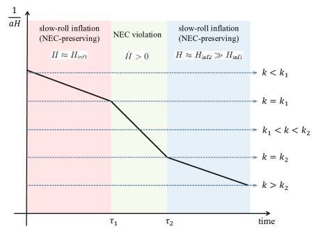
Figure 1: An illustration of the evolution of the conformal Hubble horizon (represented by the solid black lines) and the perturbation modes (depicted as dashed blue lines with arrows) in our scenario.

For the scalar (or tensor) perturbation modes that exit the horizon during the first stage of slow-roll inflation (i.e., $k<k_{1}$), their power spectrum is nearly scale-invariant, making it consistent with the observations of temperature anisotropy in the CMB. Similarly, the power spectrum of perturbation modes that exit the horizon during the second stage of slow-roll inflation (i.e., $k>k_{2}$) is also nearly scale-invariant, but it has a significantly larger amplitude. The scale-invariance of the tensor power spectrum at large scales ensures the absence of a highly suppressed tensor-to-scalar ratio $r$, and consequently a highly suppressed slow-roll parameter in canonical single-field slow-roll inflation. At small scales, the scale-invariance of the scalar and tensor power spectra prevents them from growing to $\mathcal{O}(1)$, thus preserving the validity of perturbation theory at higher frequencies.

The power spectrum of perturbation modes that exit the horizon during the NEC-violating phase (i.e., $k_{1}<k<k_{2}$) is blue-tilted ($n_{s}>0$ or $n_{T}>0$). Namely, the violation of the NEC enhances both the scalar and tensor power spectrum by increasing the Hubble parameter $H$, see Cai:2020qpu ; Cai:2022nqv ; Cai:2022lec ; Cai:2023uhc . Significantly, at the intermediate scales of the scalar power spectrum, the blue tilt and oscillatory features, particularly around the scale corresponding to the beginning of the second inflationary phase, lead to intriguing phenomena of observational interest, including the generation of primordial black holes and the associated scalar-induced GWs Cai:2023uhc . Simultaneously, the power spectrum of tensor perturbations (or the primordial GWs), also exhibits a blue tilt and possesses oscillatory features around the transition scales Cai:2020qpu ; Cai:2022nqv ; Cai:2022lec . These distinctive features set our scenario apart from other single-field primordial black hole formation scenarios. The combination of primordial black holes, scalar-induced GW signals, and primordial GWs provides a valuable avenue for studying the violation of the NEC during inflation, especially in the era of multi-messenger and multi-band observations.

Our scenario can be realized with the EFT action (see e.g., Cai:2016thi ; Cai:2017tku ; Cai:2022nqv )

$$S = \int d^{4}x\sqrt{-g}\Big{[}{M_{\rm P}^{2}\over 2}R-\Lambda(t)-c(t)g^{00}$$ (1)

$$\qquad\qquad\quad+{M_{2}^{4}(t)\over 2}(\delta g^{00})^{2}-{m_{3}^{3}(t)\over 2}\delta K\delta g^{00}+{\tilde{m}_{4}^{2}(t)\over 2}R^{(3)}\delta g^{00}\Big{]}\,,$$

where $\delta g^{00}=g^{00}+1$, $R^{(3)}$ is the Ricci scalar on the 3-dimensional spacelike hypersurface, $\delta K=K-3H$, $K$ is the extrinsic curvature. The time-dependent functions $c(t)$ and $\Lambda(t)$ determine the background evolution, with the relations $c(t)=-M_{\rm P}^{2}\dot{H}$ and $\Lambda(t)=M_{\rm P}^{2}(\dot{H}+3H^{2})$. The functions $M_{2}^{4}(t)$, $m_{3}^{3}(t)$ and $\tilde{m}_{4}^{2}(t)$ can be determined or constrained based on the condition that the scalar perturbations are in agreement with observations.

Notably, the operator $R^{(3)}\delta g^{00}$ plays a crucial role in preventing scalar perturbations from becoming unstable when the NEC is violated, as demonstrated in Cai:2016thi ; Creminelli:2016zwa ; Cai:2017tku . The covariant form of action (1), as discussed in Cai:2017dyi ; Kolevatov:2017voe , falls under the category of “beyond Horndeski” theory. Nonetheless, the propagation of primordial GWs is exactly the same as that in general relativity at quadratic order. In this paper, we will not delve into the specific formulations of these coefficient functions or the intricacies of the model construction. Instead, we will employ a simplified parameterization of the background evolution for our scenario. Consequently, we can establish a parameterization for the power spectrum of primordial GWs.

II.2 Parametrization of background

We begin with a flat Friedmann-Lemaitre-Robertson-Walker universe described by the metric

$$ds^{2}=-dt^{2}+a(t)^{2}d\vec{x}^{2}=a(\tau)^{2}(-d\tau^{2}+d\vec{x}^{2})~{},$$ (2)

where $t$ is the cosmic time and $\tau$ is the conformal time, related by $dt=ad\tau$. Throughout this paper, we will use a dot to denote $d/dt$ and a prime to denote $d/d\tau$. We will also define $H\equiv\dot{a}/a$, ${\cal H}\equiv a^{\prime}/a$.

An inflationary stage is commonly characterized by quasi-de Sitter expansion, where the scale factor approximately evolves as $a\propto|\tau|^{-1}$ for $\tau<0$. Additionally, we will parameterize our NEC-violating stage with a power-law scale factor, i.e., $a(\tau)\propto|\tau|^{n}$. The full-scale factor can be then parametrized as a piecewise function of $\tau$:

$$a_{j}(\tau)=a_{j}(\tau_{j})\left(\frac{\tau-\tau_{R,j}}{\tau_{j}-\tau_{R,j}}\right)^{\frac{1}{\epsilon_{j}-1}}~{},\quad\tau<\tau_{j}\,,$$ (3)

where $\tau_{j}$ is the conformal time at the end of phase $j$, $j=1,2,3$ corresponds to the first inflation stage, the NEC-violating stage and the second inflation stage, respectively; ${\tau}_{R,j}=\tau_{j}-(\epsilon_{j}-1)^{-1}\mathcal{H}^{-1}(\tau_{j})$ is the integration constant and $\epsilon_{j}=-\dot{H}/H^{2}$ is treated as constant during phase $j$. Since phases 1 and 3 are assumed as slow-roll inflation, we will set $\epsilon_{1}\approx\epsilon_{3}\approx 0$ for simplicity. As for the NEC-violating phase (i.e., phase 2), we have $\epsilon_{2}<0$, which indicates $-1<n=(\epsilon_{2}-1)^{-1}<0$. A specific design of such a model can be found in Cai:2020qpu .

The provided parametrization overlooks the details of transitions between different phases, including the specific variations of $\epsilon$ near the beginning or the end of the NEC-violating phase. The dynamics of the transition might depend on the specific model. For simplicity, we will describe the transition physics using the matching condition, ensuring the continuity of the scale factor $a$ and its first derivative $a^{\prime}$ at $\tau_{1}$ and $\tau_{2}$. For our purpose, such a simplification will not make a qualitative difference.

Using Eq. (3) and denoting the beginning and the end time of the NEC-violating stage to be $\tau_{1}$ and $\tau_{2}$, respectively, the continuity of $a$ gives

$$a_{1}(\tau_{1})=a_{2}(\tau_{2})\left(\frac{\tau_{1}-\tau_{R,2}}{\tau_{2}-\tau_{R,2}}\right)^{\frac{1}{\epsilon_{2}-1}}~{},~{}a_{2}(\tau_{2})=a_{3}(\tau_{3})\left(\frac{\tau_{2}-\tau_{R,3}}{\tau_{3}-\tau_{R,3}}\right)^{-1}~{}.$$ (4)

The continuity of $a^{\prime}$ or $\mathcal{H}$ enables us to define the following quantities

$$\bar{\mathcal{H}}_{1}\equiv\mathcal{H}(\tau_{1})~{},~{}\bar{\mathcal{H}}_{2}\equiv\mathcal{H}(\tau_{2})~{}.$$ (5)

With the help of (3), we can solve the integration constants as

$$\tau_{R,1}=\tau_{1}+\bar{\mathcal{H}}_{1}^{-1}~{},~{}\tau_{R,2}=\tau_{1}-\frac{\bar{\mathcal{H}}_{1}^{-1}}{\epsilon_{2}-1}=\tau_{2}-\frac{\bar{\mathcal{H}}_{2}^{-1}}{\epsilon_{2}-1}~{},~{}\tau_{R,3}=\tau_{2}+\bar{\mathcal{H}}_{2}^{-1}~{}.$$ (6)

Obviously, the consistency of (6) requires

$$(\tau_{2}-\tau_{1})(1-\epsilon_{2})=\bar{\mathcal{H}}_{1}^{-1}-\bar{\mathcal{H}}_{2}^{-1}>0~{}.$$ (7)

In terms of the scale factor and Hubble parameter;

$$\frac{a_{2}(\tau_{2})}{a_{2}(\tau_{1})}=\left(\frac{\bar{\mathcal{H}}_{2}}{\bar{\mathcal{H}}_{1}}\right)^{\frac{1}{1-\epsilon_{2}}}~{},~{}\frac{H_{2}}{H_{1}}=\left(\frac{\bar{\mathcal{H}}_{2}}{\bar{\mathcal{H}}_{1}}\right)^{\frac{\epsilon_{2}}{\epsilon_{2}-1}}~{},$$ (8)

where we have defined $H_{2}\equiv\bar{\mathcal{H}_{2}}/a_{2}(\tau_{2})$ and $H_{1}\equiv\bar{\mathcal{H}_{1}}/a_{2}(\tau_{1})$ to be the Hubble parameter at $\tau=\tau_{2}$ and $\tau=\tau_{1}$.

III Primordial gravitational waves

III.1 Tensor perturbations and mode functions

Since the gravity sector is minimally coupled to the matter sector, the quadratic action for tensor perturbation is simply

$$S_{T}^{(2)}=\int d\tau d^{3}x\frac{a^{2}}{8}\left[\gamma_{ij}^{\prime 2}-(\partial_{k}\gamma_{ij})^{2}\right]~{},$$ (9)

where we have set the propagation speed of tensor perturbation to be unity (i.e., the speed of light), and $M_{\mathrm{P}}=1$. In the momentum space, the dynamical equation for tensor perturbation is

$$u_{k}^{\prime\prime}+\left(k^{2}-\frac{a^{\prime\prime}}{a}\right)u_{k}=0~{},$$ (10)

where $u_{k}\equiv\gamma_{k}^{\lambda}a/2$ is the mode function and $\lambda=+,\times$ represent two different polarizations.

The parameterization of scale factor, i.e., Eq. (3), gives

$$\frac{a^{\prime\prime}_{j}}{a_{j}}=\frac{\nu_{j}^{2}-1/4}{(\tau-\tau_{R,j})^{2}}~{},\quad~{}\nu_{j}\equiv\frac{1}{2}+\frac{1}{1-\epsilon_{j}}~{}.$$ (11)

Note that $\epsilon_{2}<0$ would result in $1/2<\nu_{2}<3/2$. As a result, in each phase, the general solution to Eq. (10) can be expressed in terms of the Hankel function as

$$u_{k,j}(\tau)=\frac{\sqrt{\pi(\tau_{R,j}-\tau)}}{2}\left\{\alpha_{j}H_{\nu_{j}}^{(1)}[k(\tau_{R,j}-\tau)]+\beta_{j}H_{\nu_{j}}^{(2)}[k(\tau_{R,j}-\tau)]\right\}~{},$$ (12)

where $H_{\nu_{j}}^{(1)}$ and $H_{\nu_{j}}^{(2)}$ are the first and second kind Hankel functions of the $\nu_{j}$-th order, respectively; $\alpha_{j}$ and $\beta_{j}$ are $k$-dependent coefficients.

For simplicity, we have assumed $\epsilon_{1}\approx\epsilon_{3}\approx 0$, which indicates $\nu_{1}\approx\nu_{3}\approx 3/2$ and the Hankel functions are simply

$$H_{3/2}^{(1)}(x)=\sqrt{\frac{2}{\pi}}\frac{e^{ix}}{x^{3/2}}(-i-x)~{},~{}H_{3/2}^{(2)}(x)=\left[H_{3/2}^{(1)}(x)\right]^{\ast}~{},$$ (13)

where the asterisk denotes complex conjugation. We impose the Bunch-Davis vacuum initial condition, which gives $|\alpha_{1}|=1$ and $\beta_{1}=0$. The other coefficients $\alpha_{j}$ and $\beta_{j}$ for $j=2$, $3$ can be determined with the matching method, which requires the continuities of $u_{k}$ and $u_{k}^{\prime}$ at the transition surface $\tau=\tau_{1}$ and $\tau=\tau_{2}$.

More explicitly, we are interested in the final tensor spectrum, which is relevant to $|\alpha_{3}-\beta_{3}|$, namely

$$P_{T}\equiv\frac{4k^{3}}{\pi^{2}}\frac{|u_{k,3}^{2}|}{a^{2}}=\frac{2H(\tau_{3})^{2}}{\pi^{2}}|\alpha_{3}-\beta_{3}|^{2}~{}.$$ (14)

We present

$$\quad\frac{8\sqrt{x_{1}y_{1}}(\alpha_{3}-\beta_{3})}{\pi(1-2\nu_{2})}=H^{(1)}_{\nu_{2}}(y_{2})\left[\left(i-\frac{1}{x_{1}}\right)H^{(2)}_{\nu_{2}-1}(x_{2})+H^{(2)}_{\nu_{2}}(x_{2})\right]\sin y_{1}$$

$$+H^{(1)}_{\nu_{2}-1}(y_{2})\left[\left(i-\frac{1}{x_{1}}\right)H^{(2)}_{\nu_{2}-1}(x_{2})+H^{(2)}_{\nu_{2}}(x_{2})\right]\left(\cos y_{1}-\frac{\sin y_{1}}{y_{1}}\right)-$$

$$\left[\frac{ix_{1}-1}{x_{1}}H^{(1)}_{\nu_{2}-1}(x_{2})+H^{(1)}_{\nu_{2}}(x_{2})\right]\left[H^{(2)}_{\nu_{2}}(y_{2})\sin y_{1}+H^{(2)}_{\nu_{2}-1}(y_{2})\left(\cos y_{1}-\frac{\sin y_{1}}{y_{1}}\right)\right]~{},$$ (15)

see Cai:2022nqv , where we employ

$$x_{1}\equiv\frac{k}{\bar{\mathcal{H}}_{1}}~{},~{}x_{2}=\left(\nu_{2}-\frac{1}{2}\right)x_{1}~{};~{}y_{1}\equiv\frac{k}{\bar{\mathcal{H}}_{2}}~{},~{}y_{2}=\left(\nu_{2}-\frac{1}{2}\right)y_{1}~{},$$ (16)

and an overall phase factor has been neglected.

III.2 Parametrization of the tensor spectrum

The tensor spectrum provided by (III.1) is complicated, necessitating further simplification. To interpret the PTA data through primordial GWs from our model, the amplitude of primordial GWs must be enhanced from the order of $\mathcal{O}(10^{-11})$, the upper bound on the amplitude of $P_{T}$ constrained by CMB observations, to $10^{-3}$ within the PTA range. Given that in our scenario, $n_{T}<2$, the NEC violating stage must persist for scales spanning over four orders of magnitude, i.e., $k_{2}>10^{4}k_{1}$. Consequently, we can safely make the approximation $k_{2}\ll k_{1}$.

Next, we observe that the Hankel function behaves as a pure phase factor in the sub-horizon region and as a power-law function in the super-horizon region. This asymptotic behavior allows us to derive approximate expressions for modes exiting the horizon in different stages. For example, for modes exiting the horizon during the second inflation stage, where $k\gg k_{2}$, leading to $y_{1},y_{2},x_{1},x_{2}\gg 1$, each Hankel function can be approximated as a pure phase function, resulting in

$$P_{T}\simeq P_{T,2}\equiv\frac{2H_{2}^{2}}{\pi^{2}}~{},\quad k>k_{2}~{}.$$ (17)

Similarly, modes exiting the horizon during the first inflation stage satisfy $k<k_{1}$, for which we have

$$P_{T}\simeq P_{T,1}\equiv\frac{2H_{1}^{2}}{\pi^{2}}~{},\quad k<k_{1}~{}.$$ (18)

For perturbation modes that exit the horizon during the NEC-violating stage, the approximate tensor power spectrum is given by

$$P_{T}\simeq\frac{\Gamma^{2}(\nu_{2})}{\pi}\left(\frac{2\nu_{2}-1}{4}\right)^{1-2\nu_{2}}\left(\frac{k}{k_{2}}\right)^{3-2\nu_{2}}~{},\quad k_{1}<k<k_{2}~{},$$ (19)

see Cai:2022nqv for more details. This spectrum shows a blue tilt ($n_{T}=3-2\nu_{2}>0$) within the range $k_{1}<k<k_{2}$ in our scenario. Since $1/2<\nu_{2}<3/2$, we have $0<n_{T}<2$. Remarkably, when employing an exponential parameterization for $a_{2}(\tau)$, we reach $n_{T}=2$, as explicitly demonstrated in Appendix A.

The above treatment encounters challenges near the transition scales $k\simeq k_{1}$ and $k\simeq k_{2}$, where a simple expansion of the Hankel function through its asymptotic behavior is not applicable. However, in the vicinity of the scale $k\simeq k_{1}$, the corresponding tensor spectrum is expected to be too small for detection in the near future, allowing us to safely overlook the transition feature in this region. Conversely, near the scale $k\simeq k_{2}$, the tensor spectrum is sufficiently large for potential detection. For $k\gg k_{1}$, all Hankel functions with arguments $x_{1}$, $x_{2}\gg 1$ exhibit the asymptotic behavior $H_{\nu}^{(1)}(x)\propto\exp[i(x-\nu\pi/2-\pi/4)]$. This characteristic enables us to capture the features of $P_{T}$ around $k\simeq k_{2}$ while simplifying the formulation of $P_{T}$.

In light of this, we can parametrize $P_{T}$ as

$$P_{T}=P_{T,1}+\frac{\pi}{4}(2-n_{T})\frac{k}{k_{2}}|g(k)|^{2}P_{T,2}~{},$$ (20)

where the auxiliary function is defined as

$$g=H_{\frac{3-n_{T}}{2}}^{(1)}\left[\frac{2-n_{T}}{2}\frac{k}{k_{2}}\right]\sin\frac{k}{k_{2}}+H_{\frac{1-n_{T}}{2}}^{(1)}\left[\frac{2-n_{T}}{2}\frac{k}{k_{2}}\right]\left(\cos\frac{k}{k_{2}}-\frac{k_{2}}{k}\sin\frac{k}{k_{2}}\right)~{}.$$ (21)

It is important to note that we have replaced $\nu_{2}$ by the corresponding tensor spectral index $n_{T}=3-2\nu_{2}$ in the NEC violating stage. In the limit of $k\ll k_{1}$, $P_{T}\approx P_{T,1}$ since the second term in Eq. (20) becomes negligible compared to $P_{T,1}$. Conversely, for $k\gg k_{1}$, the second term in Eq. (20) becomes dominant. Consequently, it ensures that the features around $k\simeq k_{2}$ are well captured. While this formulation may sacrifice accuracy around the first transition scale $k\simeq k_{1}$, such a compromise has minimal impact on our interests.

The primordial tensor power spectrum $P_{T}$ can be converted to the observed GW energy spectrum by Turner:1993vb

$$\Omega_{\rm{GW}} =\frac{k^{2}}{12a_{0}^{2}H_{0}^{2}}\left[\frac{3\Omega_{m}j_{l}(k\tau_{0})}{k\tau_{0}}\sqrt{1.0+1.36\frac{k}{k_{eq}}+2.50\left(\frac{k}{k_{eq}}\right)^{2}}\right]^{2}P_{T}$$ (22)

$$\simeq\frac{1}{24}\left(\frac{k}{H_{0}}\right)^{2}\left[\frac{3\Omega_{m}}{(k\tau_{0})^{2}}\sqrt{1.0+1.36\frac{k}{k_{eq}}+2.50\left(\frac{k}{k_{eq}}\right)^{2}}\right]^{2}P_{T}$$

where $H_{0}=67.8\,{\rm km/s/Mpc}$, $\tau_{0}=1.41\times 10^{4}$ Mpc, $a_{0}=1$, $k_{\text{eq}}=0.073\,\Omega_{\text{m}}h^{2}$ Mpc^-1, $\Omega_{\rm m}$ is the density fraction of matter today, and the wavenumber relates to the frequency as $k=2\pi f$.

IV Numerical results

In this section, we confront the parameterized spectrum (20) to the recent PTA data. As explained in the previous section, we are interested in the case $k_{1}\ll k\lesssim k_{2}$ where the tensor spectrum is blue. To this end, the first term in (20) is much smaller than the second one, thus we can safely neglect $P_{T,1}$. With this simplification, the theoretical spectrum (20) is fully parameterized by three parameters $\{P_{T,2},\ n_{T},\ f_{c}\}$, where we have defined the transition frequency from the NEC-violating stage to the second inflationary stage as $f_{c}\equiv 2\pi k_{2}$. We performed Monte Carlo Markov Chain (MCMC) analysis varying $\{P_{T,2},\ n_{T},\ f_{c}\}$ plus the pulsar and nuisance parameters against the most recent public NANOGrav 15yr dataset NANOGrav:2023gor . Following NANOGrav, we assume two models on the spatial correlation of the signal, uncorrelated common-spectrum red noise (CURN) and Hellings-Down (HD).. Theoretically, our model predicts $n_{T}<2$. The validity of the perturbation theory requires $P_{T,2}<1$. See Table.1 for our prior choice of the model parameters.

Fig.2 shows the posterior distributions of the tensor spectrum parameters. Data puts lower bounds on $P_{T,2}>10^{-2}$ (95% C.L.) and $n_{T}>1.0$ (95% C.L.). This is to be expected because it is known that the NANOGrav 15yr data includes a $\sim 3\sigma$ detection of GW background near $10^{-8}$ Hz with $n_{T}\sim 1.8$. The distribution of $f_{c}$ is a peak $-8.1<\log_{10}(f_{c}/\mathrm{Hz})<-6.6$, but this should not be confused with a detection. Near $f_{c}$, the spectrum transits from $n_{T}\sim 2$ to $n_{T}=0$ with oscillations. Having $f_{c}>10^{-8}$ Hz means that data does not favor the shape of transition so it is moved to the right of the data constraining region, see also Fig.3. The upper bound on $f_{c}$ is due to the prior upper bound on $P_{T,2}$. Because data fixes the amplitude of the spectrum near $10^{-8}$ Hz, $f_{c}$ and $P_{T,2}$ are strongly positively correlated, as can be seen from the $\log_{10}f_{c}$ - $\log_{10}P_{T,2}$ contour of Fig.2. Therefore, a prior upper bound $P_{T,2}<1$ gets translated to an upper bound on $f_{c}$.

Fig.3 further compares the best-fit theoretical spectrum with violin points measured by NANOGrav. The left panel of Fig.3 illustrates the physical energy spectrum of GW denoted as $\Omega_{GW}h^{2}$. While the NEC-violating phase satisfactorily accounts for the PTA signal, the tensor spectrum originating from the second inflationary phase also falls comfortably within the detection sensitivity of forthcoming space-based GW observatories like LISA LISA:2017pwj , Taiji Hu:2017mde , and Tianqin TianQin:2015yph . The right panel of Fig.3 zooms into the PTA data-constrained frequency range and plots the PTA timing excess, see NANOGrav:2023gor for a detailed definition. Only the first few data points detect GW background signal and the theoretical spectrum (solid black line) fits them as well as a power law (dashed black line). Close to $f_{c}$, the solid line drops to a smaller $n_{T}$, which is not favored by data. Therefore, in the MCMC, $f_{c}$ automatically shifts to a higher frequency than the range constrained by the data, leading to the observed lower bound on $f_{c}$ as depicted in Fig.2.

The numeric results confirmed that the NEC-violating model can well explain the GW background signal observed by PTA experiments, but the current data is not precise enough to distinguish it from other models, e.g., a simple power law. Our model also predicts a flat tensor spectrum in the mHz frequency range and is detectable to next-generation space GW detectors.

Parameter	Prior
$\log_{10}P_{T,2}$	[-5,0]
$n_{T}$	$[0,2]$
$\log_{10}f_{c}$	[-9,-5]

Table 1: Prior choice for spectrum parameters in the MCMC analysis.

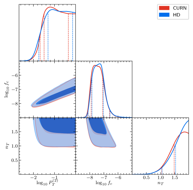
Figure 2: 68% and 95% posterior distributions of model parameters.

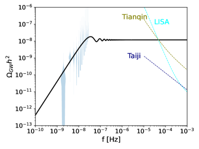
(a)   $\Omega_{\text{GW}}h^{2}$

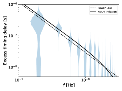
(b)   Excess timing

Figure 3: Theoretical spectra with violin data points from NANOGrav 15yr.

V Conclusions

The recent SGWB signals reported by PTA collaborations have unveiled a new frontier in the exploration of gravitational wave physics. Notably, if these PTA signals originate from the primordial universe, it necessitates the presence of new physics beyond the standard slow-roll inflation scenario. This necessity arises because PTA observations indicate a highly blue tensor spectrum with a spectral index of $n_{T}=1.8\pm 0.3$, whereas the conventional slow-roll inflation scenario predicts a nearly scale-invariant tensor spectrum.

An intermediate stage of NEC violation during inflation has the potential to amplify the primordial tensor power spectrum on certain scales, offering a potential explanation for the PTA observations. In this paper, we explore the primordial GW spectrum within an inflationary scenario featuring an intermediate NEC-violating phase. We present parameterizations for the background evolution and the GW power spectrum of our model. Our evaluation of the model’s compatibility with PTA data reveals its capability to account for the SGWB signal observed by PTA experiments. Given the consistency of signals observed by various PTA experiments, we focus primarily on the NANOGrav 15-year results in the numerical analysis.

Additionally, our model predicts a nearly scale-invariant GW spectrum in the mHz frequency range, potentially detectable by upcoming space-based GW detectors like LISA, Taiji, and Tianqin. This distinctive characteristic distinguishes our scenario from other interpretations predicting a red primordial GW spectrum on smaller scales.

VI Discussions

Intriguingly, Ref. Cai:2022lec found that, for the scenario discussed in this paper, the violation of the NEC naturally amplifies the parity-violating effect as well as its observability in primordial GWs, provided the scalar field determining the background evolution is coupled to a parity-violating term. The wavenumber $k$ corresponding to the maximum of the parity-violating effect is approximately the same as the wavenumber corresponding to the maximum of the power spectrum. This intriguing feature also sets our model apart observationally from other models.

The scale corresponding to the significantly amplified parity-violating effects depends on the scale at which the NEC violation takes place. In this paper, the maximum of the primordial GW power spectrum appears in the vicinity of the PTA band, as shown by the black curve in Fig. 3. Therefore, the parity violation is still notably amplified in the PTA band. However, considering the power spectrum presented in Fig. 3, the parity violation is suppressed by the slow-roll condition in the LISA band, as the GW modes in the LISA band are generated during the second slow-roll inflation stage in our scenario. To achieve a notable amplification of the parity-violating effect in the LISA band, it would be necessary for the NEC violation to occur later than what is assumed in the present paper.

In Ref. Cai:2023uhc , it has been demonstrated that the NEC violation can naturally enhance the primordial scalar power spectrum at certain scales, leading to the production of PBHs and scalar-induced GWs of observational interest. The primordial GWs (i.e., tensor perturbations) primarily depend on the Hubble parameter $H$. The scalar-induced GWs are induced by scalar perturbations, depending not only on $H$ but also on $\epsilon\equiv-\dot{H}/H^{2}$ (or its generalized formulation). Therefore, the relative contribution to the GW background of each depends on the specific model’s characteristics, particularly the relative magnitudes of the power spectra of scalar and tensor perturbations.

In this paper, we primarily focus on primordial GWs and have not explicitly calculated the primordial scalar perturbations. We assume that the contribution to the GW background in the PTA band mainly comes from primordial GWs rather than scalar-induced GWs. In fact, for the same background evolution, scalar perturbations exhibit stronger model dependence compared to tensor perturbations. In principle, for models constructed with specific covariant action, we can quantitatively compare the contributions of both to the GW background. This remains a subject for future work.

Appendix A Power spectrum from an exponential parameterization of the scale factor during the NEC-violating phase

In this section, we explicitly calculate the power spectrum $P_{T}$ using an exponential parameterization for $a_{2}(\tau)$, representing the scale factor during the NEC-violating stage. This parametrization is frequently used in the study of bouncing cosmology, which also has an NEC-violating phase, see e.g., Cai:2012va .

The first and second inflationary stages, denoted by $i=1$ and $3$ respectively, are still parameterized by Eq. (3), with the assumption that $\epsilon_{1}\approx\epsilon_{3}\approx 0$. Therefore, we have

$$a_{1}(\tau)=a_{1}(\tau_{1})\frac{\tau_{1}-\tau_{R,1}}{\tau-\tau_{R,1}}~{},~{}\mathcal{H}_{1}(\tau)=-\frac{1}{\tau-\tau_{R,1}}~{},~{}\tau\leq\tau_{1}$$ (23)

and

$$a_{3}(\tau)=a_{3}(\tau_{3})\frac{\tau_{3}-\tau_{R,3}}{\tau-\tau_{R,3}}~{},~{}\mathcal{H}_{3}(\tau)=-\frac{1}{\tau-\tau_{R,3}}~{},~{}\tau_{2}\leq\tau\leq\tau_{3}$$ (24)

If the NEC-violating phase is very brief, we can approximate the Hubble parameter as a linear function. As a result, $a_{2}(\tau)$ can be parameterized by an exponential formulation as

$$a_{2}(\tau)=a_{1}(\tau_{1})e^{\mathcal{H}_{1}(\tau_{1})(\tau-\tau_{1})+\frac{1}{2}\gamma^{2}(\tau-\tau_{1})^{2}}~{},~{}\mathcal{H}_{2}(\tau)=\mathcal{H}_{1}(\tau_{1})+\gamma^{2}(\tau-\tau_{1})~{},$$ (25)

where $\tau_{1}\leq\tau\leq\tau_{2}$.

The parameterization of the background can be related to the characteristic scales:

$$k_{1}=\mathcal{H}_{1}(\tau_{1})=(\tau_{R,1}-\tau_{1})^{-1}~{},~{}k_{2}=\mathcal{H}_{3}(\tau_{2})=(\tau_{R,3}-\tau_{2})^{-1}~{},$$ (26)

where $k_{1}$ is the mode that crosses the horizon at the end of the first inflationary phase, $\tau=\tau_{1}$, and $k_{2}$ is the mode that crosses the horizon at the beginning of the second inflationary phase, $\tau=\tau_{2}$.

The continuity of $a$ and $\mathcal{H}$ at $\tau_{1}$ is already incorporated into the parametrization. Therefore, we focus on ensuring continuity at $\tau_{2}$, which requires that $a_{3}(\tau_{2})=a_{2}(\tau_{2})$ and $\mathcal{H}_{3}(\tau_{2})=\mathcal{H}_{2}(\tau_{2})$, i.e.,

$$\frac{a_{3}(\tau_{2})}{a_{1}(\tau_{1})}=e^{\mathcal{H}_{1}(\tau_{1})(\tau_{2}-\tau_{1})+\frac{1}{2}\gamma^{2}(\tau_{2}-\tau_{1})^{2}}~{},~{}-\frac{1}{\tau_{2}-\tau_{R,3}}=\mathcal{H}_{1}(\tau_{1})+\gamma^{2}(\tau_{2}-\tau_{1})~{}.$$ (27)

In terms of $k_{1}$ and $k_{2}$, and considering the condition $k_{1}\ll k_{2}$, we can express

$$k_{2}=k_{1}+\gamma^{2}(\tau_{2}-\tau_{1})\simeq\gamma^{2}(\tau_{2}-\tau_{1})~{},$$ (28)

leading to

$$\tau_{2}-\tau_{1}\simeq\frac{k_{2}}{\gamma^{2}},\frac{a_{3}(\tau_{2})}{a_{1}(\tau_{1})}\simeq e^{\frac{k_{2}}{2\gamma^{2}}(k_{2}+2k_{1})}\simeq e^{\frac{k_{2}^{2}}{2\gamma^{2}}}~{}.$$ (29)

For the first inflationary phase (i.e., $\tau<\tau_{1}$), the mode function can be given as

$$u_{k,1}(\tau)=\frac{\sqrt{\pi(\tau_{R,1}-\tau)}}{2}H_{3/2}^{(1)}[k(\tau_{R,1}-\tau)]=\frac{e^{ik(\tau_{R,1}-\tau)}}{\sqrt{2}k^{3/2}(\tau_{R,1}-\tau)}[-i-k(\tau_{R,1}-\tau)]~{},$$ (30)

where we have taken the vacuum initial condition. It can be further simplified to

$$u_{k,1}(\tau)=-\frac{k+ik_{1}}{\sqrt{2}k^{3/2}}e^{\frac{ik}{k_{1}}}~{},~{}~{}\tau<\tau_{1}~{}.$$ (31)

In the NEC-violating phase, we have $\epsilon\equiv 1-{\mathcal{H}^{\prime}}/{\mathcal{H}^{2}}\ll-1$, indicating $\mathcal{H}^{\prime}\gg\mathcal{H}^{2}$ for nearly the entire phase. As a result, ${a^{\prime\prime}}/{a}=\mathcal{H}^{2}+\mathcal{H}^{\prime}\simeq\mathcal{H}^{\prime}=\gamma^{2}$. Consequently, the dynamical equation simplifies to

$$u_{k,2}^{\prime\prime}(\tau)-\omega_{k}^{2}u_{k,2}(\tau)=0,\omega_{k}\equiv\sqrt{\gamma^{2}-k^{2}}~{}.$$ (32)

The parameter $\omega_{k}$ turns imaginary for $k>\gamma$ and real for $k<\gamma$. Yet, we will primarily focus on analyzing the dynamics of perturbations for $k<\gamma$ as it should be adequate for our purposes. In this scenario, $\omega_{k}$ is real, and the general solution takes the form

$$u_{k,2}=c_{1}e^{\omega_{k}\tau}+c_{2}e^{-\omega_{k}\tau}~{}.$$ (33)

The mode function for the second inflationary phase can be expressed as

$$u_{k,3}(\tau)=c_{3}\sqrt{\frac{\pi(\tau_{R,3}-\tau)}{2}}J_{\frac{3}{2}}[k(\tau_{R,3}-\tau)]+c_{4}\sqrt{\frac{\pi(\tau_{R,3}-\tau)}{2}}Y_{\frac{3}{2}}[k(\tau_{R,3}-\tau)]~{},$$ (34)

where $J$ and $Y$ are Bessel functions. In a more explicit form, this can be written as

$$u_{k,3}(\tau)=c_{3}\left(\frac{\sin z}{z}-\cos z\right)-c_{4}\left(\frac{\cos z}{z}+\sin z\right)~{},$$ (35)

where $z\equiv k(\tau_{R,3}-\tau)$. On super-horizon scales, the dominating term is $c_{4}$, making it sufficient to evaluate $c_{4}$. The tensor spectrum on these scales, expressed in terms of $c_{4}$, is given by

$$P_{T}=\frac{4k^{3}}{\pi^{2}}\frac{|u_{k,3}^{2}|}{a^{2}}=\frac{2H_{\text{inf,2}}^{2}}{\pi^{2}}2k|c_{4}|^{2}~{}.$$ (36)

We match the perturbation at $\tau_{1}$ and $\tau_{2}$ for fluctuations with $k<\gamma$, resulting in

$$c_{4} =\frac{k^{2}+(ik-k_{1})(k_{1}+\omega_{k})}{2\sqrt{2}k^{7/2}\omega_{k}}e^{\frac{\omega_{k}}{k_{2}}}\Bigg{[}k^{2}\sin\frac{k}{k_{2}}$$

$$+(k_{2}-\omega_{k})\left(k\cos\frac{k}{k_{2}}-k_{2}\sin\frac{k}{k_{2}}\right)\Bigg{]}+(\omega_{k}\to-\omega_{k})~{}.$$ (37)

A quick check: for modes crossing the horizon in the first inflation phase, we have $k<k_{1}\ll k_{2}$. Moreover, the largeness of $|\epsilon|$ implies $|\epsilon|(\tau_{1})=1-\frac{\gamma^{2}}{k_{1}^{2}}\gg 1$, or $\gamma\gg k_{1}\geq k$, and thus $\omega_{k}\simeq\gamma$. A series expansion around $k/k_{2}\ll 1$ gives

$$c_{4}\simeq\frac{(ik-k_{1})}{6\sqrt{2}k_{2}^{2}k^{\frac{1}{2}}}e^{\frac{\gamma}{k_{2}}}\left(2k_{2}+\gamma\right)+(\gamma\to-\gamma)~{}.$$ (38)

Therefore, for $k\ll k_{1}$, the power spectrum is

$$P_{T,\text{inf1}} \simeq\frac{2H_{\text{inf,2}}^{2}}{\pi^{2}}\times\frac{k_{1}^{2}}{k_{2}^{2}}\left[\frac{1}{6}e^{\frac{\gamma}{k_{2}}}\left(2+\frac{\gamma}{k_{2}}\right)+(\gamma\to-\gamma)\right]^{2}$$

$$=\frac{2H_{\text{inf,1}}^{2}}{\pi^{2}}\frac{a_{1}^{2}}{a_{2}^{2}}\left[\frac{1}{6}e^{\frac{\gamma}{k_{2}}}\left(2+\frac{\gamma}{k_{2}}\right)+(\gamma\to-\gamma)\right]^{2}$$

$$\simeq\frac{2H_{\text{inf,1}}^{2}}{\pi^{2}}\left[\frac{1}{6}\left(2+\frac{\gamma}{k_{2}}\right)+\frac{a_{1}}{a_{2}}\left(2-\frac{\gamma}{k_{2}}\right)\right]^{2}\simeq P_{T,\text{inf1}}\left(\frac{1}{3}+\frac{\gamma}{6k_{2}}\right)^{2}~{},$$ (39)

which is scale-invariant, as expected. The equation (A) indicates that the super-horizon modes generally experience a modification factor during the NEC-violating phase, aligning with results from bouncing cosmology.

Modes with $k>k_{2}$ and $k>\gamma$ remain sub-horizon at $\tau=\tau_{2}$ and cross the horizon in the second inflationary phase. Therefore, we can directly write down their corresponding tensor spectrum:

$$P_{T,\text{inf2}}\simeq\frac{2H_{\text{inf,2}}^{2}}{\pi^{2}}~{}.$$ (40)

To explain the PTA result, we aim for $P_{T,\text{inf2}}\simeq\mathcal{O}(10^{-4})$. The CMB constraint gives $P_{T,\text{inf1}}\simeq\mathcal{O}(10^{-12})$. Consequently, we can estimate $H_{\text{inf,2}}/H_{\text{inf,1}}>\mathcal{O}(10^{4})$. This estimation provides us with an estimate for $\gamma$, i.e.,

$$\frac{H_{\text{inf,2}}}{H_{\text{inf,1}}}=\frac{\mathcal{H}_{2}}{\mathcal{H}_{1}}\frac{a_{1}}{a_{2}}>\mathcal{O}(10^{4})~{}\to~{}\frac{k_{2}}{k_{1}}e^{\frac{k_{2}^{2}}{2\gamma^{2}}}>\mathcal{O}(10^{4})~{}.$$ (41)

The exponential function is sensitive to the value of $k_{2}/\gamma$, which suggests that $k_{2}$ and $\gamma$ have the same order of magnitude. For example, if $k_{2}/\gamma=10$, it would imply an amplification of the Hubble parameter by $e^{50}$, an implausible result. Therefore, we could reasonably approximate $P_{T}=P_{T,\text{inf2}}$ for $k>\gamma$, accepting a minor loss of precision within a narrow scale range.

Obtaining the tensor spectrum for $k>\gamma$ from (A) via analytical continuation on $\omega_{k}$ might raise a potential issue. The expression for $c_{4}$ displays an apparent discontinuity at $k=\gamma$ and$\omega_{k}=0$. Looking into this issue in the limit of $k\to\gamma$, we find

$$\lim_{k\to\gamma}c_{4}\simeq\frac{\left(\gamma^{2}-k_{2}^{2}\right)\sin\frac{\gamma}{k_{2}}+\gamma k_{2}\cos\frac{\gamma}{k_{2}}}{\sqrt{2}\gamma^{\frac{3}{2}}k_{2}}~{}.$$ (42)

Therefore, $c_{4}$ is well-defined at $k=\gamma$. Moreover, for $k\gg\gamma$,

$$c_{4}\simeq\frac{1}{2\sqrt{2}k^{\frac{3}{2}}}\left\{\frac{e^{\frac{i|\omega_{k}|}{k_{2}}}}{i|\omega_{k}|}\left[k^{2}\sin\frac{k}{k_{2}}-i|\omega_{k}|\left(k\cos\frac{k}{k_{2}}-k_{2}\sin\frac{k}{k_{2}}\right)\right]+c.c.\right\}~{}.$$ (43)

Using $|\omega_{k}|\simeq k$, it can be further simplified to

$$|c_{4}|=\frac{1}{\sqrt{2}k^{\frac{1}{2}}}\left|1+\mathcal{O}\left(\frac{k_{2}}{k}\right)\right|\to P_{T}\simeq\frac{2H_{\text{inf,2}}^{2}}{\pi^{2}}=P_{T,\text{inf2}}~{}.$$ (44)

Therefore, we can evaluate $P_{T}$ with $k>\gamma$ through the analytical continuation of $\omega_{k}$, which we verified numerically and illustrate in Fig. 4.

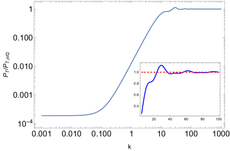
Figure 4: The tensor power spectrum with $k_{1}=0.12$, $k_{2}=10$, $\gamma=8$.

In conclusion, we could adopt the following parametrization for $P_{T}$:

$$P_{T}=\frac{H_{\text{inf,2}}^{2}}{2\pi^{2}}|f(k)^{2}|~{},$$ (45)

where

$$f(k) =\frac{k^{2}+(ik-k_{1})(k_{1}+\omega_{k})}{k^{3}\omega_{k}}e^{\frac{\omega_{k}}{k_{2}}}\Bigg{[}(k_{2}-\omega_{k})\left(k\cos\frac{k}{k_{2}}-k_{2}\sin\frac{k}{k_{2}}\right)$$

$$+k^{2}\sin\frac{k}{k_{2}}\Bigg{]}+(\omega_{k}\to-\omega_{k})~{},~{}\omega_{k}\equiv\sqrt{\gamma^{2}-k^{2}}~{}.$$ (46)

How does this relate to PTA observations? As we can see from Fig. 4, the tensor spectrum is blue-tilted in the region $k_{1}\ll k\ll k_{2}$. Since $\gamma$ is comparable to $k_{2}$, we also have $\gamma\gg k$ such that $\omega_{k}\simeq\gamma$. The expression (A) simplifies to

$$|f(k)|\simeq\frac{k}{3k_{2}^{2}}\left[(2k_{2}+\gamma)e^{\frac{\gamma}{k_{2}}}+(2k_{2}-\gamma)e^{-\frac{\gamma}{k_{2}}}\right]~{},$$ (47)

which predicts a blue spectrum with $n_{T}=2$ in the range $k_{1}\ll k\ll k_{2}$. This result is in agreement with that in the main text in the limit $n\to\infty$, as the power-law parametrization $a_{2}\propto|\tau|^{n}$ approaches an exponential function.

However, when $k\sim\gamma$ and $\gamma\neq k_{2}$, we also observe a blue spectrum from Fig. 4. Yet, estimating the spectral index analytically becomes challenging in this scenario as we lack a reliable method to estimate $\omega_{k}$.

References

- (1) S. L. Detweiler, “Pulsar timing measurements and the search for gravitational waves,” Astrophys. J. 234 (1979) 1100–1104.
- (2) LIGO Scientific, Virgo Collaboration, B. P. Abbott et al., “Observation of Gravitational Waves from a Binary Black Hole Merger,” Phys. Rev. Lett. 116 no. 6, (2016) 061102, arXiv:1602.03837 [gr-qc].
- (3) NANOGrav Collaboration, A. Afzal et al., “The NANOGrav 15 yr Data Set: Search for Signals from New Physics,” Astrophys. J. Lett. 951 no. 1, (2023) L11, arXiv:2306.16219 [astro-ph.HE].
- (4) NANOGrav Collaboration, G. Agazie et al., “The NANOGrav 15 yr Data Set: Evidence for a Gravitational-wave Background,” Astrophys. J. Lett. 951 no. 1, (2023) L8, arXiv:2306.16213 [astro-ph.HE].
- (5) EPTA Collaboration, J. Antoniadis et al., “The second data release from the European Pulsar Timing Array III. Search for gravitational wave signals,” Astron. Astrophys. 678 (2023) A50, arXiv:2306.16214 [astro-ph.HE].
- (6) D. J. Reardon et al., “Search for an Isotropic Gravitational-wave Background with the Parkes Pulsar Timing Array,” Astrophys. J. Lett. 951 no. 1, (2023) L6, arXiv:2306.16215 [astro-ph.HE].
- (7) H. Xu et al., “Searching for the Nano-Hertz Stochastic Gravitational Wave Background with the Chinese Pulsar Timing Array Data Release I,” Res. Astron. Astrophys. 23 no. 7, (2023) 075024, arXiv:2306.16216 [astro-ph.HE].
- (8) A. Addazi, Y.-F. Cai, A. Marciano, and L. Visinelli, “Have pulsar timing array methods detected a cosmological phase transition?,” arXiv:2306.17205 [astro-ph.CO].
- (9) N. Kitajima and K. Nakayama, “Nanohertz gravitational waves from cosmic strings and dark photon dark matter,” arXiv:2306.17390 [hep-ph].
- (10) P. Athron, A. Fowlie, C.-T. Lu, L. Morris, L. Wu, Y. Wu, and Z. Xu, “Can Supercooled Phase Transitions explain the Gravitational Wave Background observed by Pulsar Timing Arrays?,” arXiv:2306.17239 [hep-ph].
- (11) A. Ghoshal and A. Strumia, “Probing the Dark Matter density with gravitational waves from super-massive binary black holes,” arXiv:2306.17158 [astro-ph.CO].
- (12) J. Yang, N. Xie, and F. P. Huang, “Nano-Hertz stochastic gravitational wave background as hints of ultralight axion particles,” arXiv:2306.17113 [hep-ph].
- (13) Y. Bai, T.-K. Chen, and M. Korwar, “QCD-Collapsed Domain Walls: QCD Phase Transition and Gravitational Wave Spectroscopy,” arXiv:2306.17160 [hep-ph].
- (14) J. Ellis, M. Fairbairn, G. Hütsi, J. Raidal, J. Urrutia, V. Vaskonen, and H. Veermäe, “Gravitational Waves from SMBH Binaries in Light of the NANOGrav 15-Year Data,” arXiv:2306.17021 [astro-ph.CO].
- (15) H.-L. Huang, Y. Cai, J.-Q. Jiang, J. Zhang, and Y.-S. Piao, “Supermassive primordial black holes in multiverse: for nano-Hertz gravitational wave and high-redshift JWST galaxies,” arXiv:2306.17577 [gr-qc].
- (16) G. Franciolini, A. Iovino, Junior., V. Vaskonen, and H. Veermae, “The recent gravitational wave observation by pulsar timing arrays and primordial black holes: the importance of non-gaussianities,” arXiv:2306.17149 [astro-ph.CO].
- (17) Y. Li, C. Zhang, Z. Wang, M. Cui, Y.-L. S. Tsai, Q. Yuan, and Y.-Z. Fan, “Primordial magnetic field as a common solution of nanohertz gravitational waves and Hubble tension,” arXiv:2306.17124 [astro-ph.HE].
- (18) N. Kitajima, J. Lee, K. Murai, F. Takahashi, and W. Yin, “Nanohertz Gravitational Waves from Axion Domain Walls Coupled to QCD,” arXiv:2306.17146 [hep-ph].
- (19) S. Datta and R. Samanta, “Fingerprints of GeV scale right-handed neutrinos on inflationary gravitational waves and PTA data,” Phys. Rev. D 108 no. 9, (2023) L091706, arXiv:2307.00646 [hep-ph].
- (20) K. Fujikura, S. Girmohanta, Y. Nakai, and M. Suzuki, “NANOGrav Signal from a Dark Conformal Phase Transition,” arXiv:2306.17086 [hep-ph].
- (21) S. Vagnozzi, “Inflationary interpretation of the stochastic gravitational wave background signal detected by pulsar timing array experiments,” arXiv:2306.16912 [astro-ph.CO].
- (22) J. Ellis, M. Lewicki, C. Lin, and V. Vaskonen, “Cosmic Superstrings Revisited in Light of NANOGrav 15-Year Data,” arXiv:2306.17147 [astro-ph.CO].
- (23) Z. Wang, L. Lei, H. Jiao, L. Feng, and Y.-Z. Fan, “The nanohertz stochastic gravitational-wave background from cosmic string Loops and the abundant high redshift massive galaxies,” arXiv:2306.17150 [astro-ph.HE].
- (24) S.-Y. Guo, M. Khlopov, X. Liu, L. Wu, Y. Wu, and B. Zhu, “Footprints of Axion-Like Particle in Pulsar Timing Array Data and JWST Observations,” arXiv:2306.17022 [hep-ph].
- (25) C. Han, K.-P. Xie, J. M. Yang, and M. Zhang, “Self-interacting dark matter implied by nano-Hertz gravitational waves,” arXiv:2306.16966 [hep-ph].
- (26) Z.-Q. Shen, G.-W. Yuan, Y.-Y. Wang, and Y.-Z. Wang, “Dark Matter Spike surrounding Supermassive Black Holes Binary and the nanohertz Stochastic Gravitational Wave Background,” arXiv:2306.17143 [astro-ph.HE].
- (27) L. Zu, C. Zhang, Y.-Y. Li, Y.-C. Gu, Y.-L. S. Tsai, and Y.-Z. Fan, “Mirror QCD phase transition as the origin of the nanohertz Stochastic Gravitational-Wave Background detected by the Pulsar Timing Arrays,” arXiv:2306.16769 [astro-ph.HE].
- (28) Y.-C. Bi, Y.-M. Wu, Z.-C. Chen, and Q.-G. Huang, “Implications for the Supermassive Black Hole Binaries from the NANOGrav 15-year Data Set,” arXiv:2307.00722 [astro-ph.CO].
- (29) S. Wang, Z.-C. Zhao, J.-P. Li, and Q.-H. Zhu, “Exploring the Implications of 2023 Pulsar Timing Array Datasets for Scalar-Induced Gravitational Waves and Primordial Black Holes,” arXiv:2307.00572 [astro-ph.CO].
- (30) T. Broadhurst, C. Chen, T. Liu, and K.-F. Zheng, “Binary Supermassive Black Holes Orbiting Dark Matter Solitons: From the Dual AGN in UGC4211 to NanoHertz Gravitational Waves,” arXiv:2306.17821 [astro-ph.HE].
- (31) Y.-F. Cai, X.-C. He, X. Ma, S.-F. Yan, and G.-W. Yuan, “Limits on scalar-induced gravitational waves from the stochastic background by pulsar timing array observations,” arXiv:2306.17822 [gr-qc].
- (32) P. F. Depta, K. Schmidt-Hoberg, and C. Tasillo, “Do pulsar timing arrays observe merging primordial black holes?,” arXiv:2306.17836 [astro-ph.CO].
- (33) L. Bian, S. Ge, J. Shu, B. Wang, X.-Y. Yang, and J. Zong, “Gravitational wave sources for Pulsar Timing Arrays,” arXiv:2307.02376 [astro-ph.HE].
- (34) G. Franciolini, D. Racco, and F. Rompineve, “Footprints of the QCD Crossover on Cosmological Gravitational Waves at Pulsar Timing Arrays,” arXiv:2306.17136 [astro-ph.CO].
- (35) X. K. Du, M. X. Huang, F. Wang, and Y. K. Zhang, “Did the nHZ Gravitational Waves Signatures Observed By NANOGrav Indicate Multiple Sector SUSY Breaking?,” arXiv:2307.02938 [hep-ph].
- (36) Y.-M. Wu, Z.-C. Chen, and Q.-G. Huang, “Cosmological Interpretation for the Stochastic Signal in Pulsar Timing Arrays,” arXiv:2307.03141 [astro-ph.CO].
- (37) Z. Yi, Q. Gao, Y. Gong, Y. Wang, and F. Zhang, “The waveform of the scalar induced gravitational waves in light of Pulsar Timing Array data,” arXiv:2307.02467 [gr-qc].
- (38) Z.-C. Liang, Z.-Y. Li, E.-K. Li, J.-d. Zhang, and Y.-M. Hu, “Sensitivity to anisotropic stochastic gravitational-wave background with space-borne networks,” arXiv:2307.01541 [gr-qc].
- (39) L. A. Anchordoqui, I. Antoniadis, and D. Lust, “Fuzzy Dark Matter, the Dark Dimension, and the Pulsar Timing Array Signal,” arXiv:2307.01100 [hep-ph].
- (40) E. Battista, V. De Falco, and D. Usseglio, “First post-Newtonian N-body problem in Einstein–Cartan theory with the Weyssenhoff fluid: Lagrangian and first integrals,” Eur. Phys. J. C 83 no. 2, (2023) 112, arXiv:2301.08954 [gr-qc].
- (41) V. De Falco and E. Battista, “Analytical results for binary dynamics at the first post-Newtonian order in Einstein-Cartan theory with the Weyssenhoff fluid,” Phys. Rev. D 108 no. 6, (2023) 064032, arXiv:2309.00319 [gr-qc].
- (42) S.-P. Li and K.-P. Xie, “Collider test of nano-Hertz gravitational waves from pulsar timing arrays,” Phys. Rev. D 108 no. 5, (2023) 055018, arXiv:2307.01086 [hep-ph].
- (43) Y. Xiao, J. M. Yang, and Y. Zhang, “Implications of Nano-Hertz Gravitational Waves on Electroweak Phase Transition in the Singlet Dark Matter Model,” arXiv:2307.01072 [hep-ph].
- (44) C. Zhang, N. Dai, Q. Gao, Y. Gong, T. Jiang, and X. Lu, “Detecting new fundamental fields with Pulsar Timing Arrays,” arXiv:2307.01093 [gr-qc].
- (45) L. Liu, Z.-C. Chen, and Q.-G. Huang, “Implications for the non-Gaussianity of curvature perturbation from pulsar timing arrays,” arXiv:2307.01102 [astro-ph.CO].
- (46) K. Inomata, K. Kohri, and T. Terada, “The Detected Stochastic Gravitational Waves and Subsolar-Mass Primordial Black Holes,” arXiv:2306.17834 [astro-ph.CO].
- (47) T. Ghosh, A. Ghoshal, H.-K. Guo, F. Hajkarim, S. F. King, K. Sinha, X. Wang, and G. White, “Did we hear the sound of the Universe boiling? Analysis using the full fluid velocity profiles and NANOGrav 15-year data,” arXiv:2307.02259 [astro-ph.HE].
- (48) X. Niu and M. H. Rahat, “NANOGrav signal from axion inflation,” arXiv:2307.01192 [hep-ph].
- (49) R. A. Konoplya and A. Zhidenko, “Asymptotic tails of massive gravitons in light of pulsar timing array observations,” arXiv:2307.01110 [gr-qc].
- (50) P. Di Bari and M. H. Rahat, “The split majoron model confronts the NANOGrav signal,” arXiv:2307.03184 [hep-ph].
- (51) S. Wang, Z.-C. Zhao, and Q.-H. Zhu, “Constraints On Scalar-Induced Gravitational Waves Up To Third Order From Joint Analysis of BBN, CMB, And PTA Data,” arXiv:2307.03095 [astro-ph.CO].
- (52) G. Ye and A. Silvestri, “Can the gravitational wave background feel wiggles in spacetime?,” arXiv:2307.05455 [astro-ph.CO].
- (53) S. Balaji, G. Domènech, and G. Franciolini, “Scalar-induced gravitational wave interpretation of PTA data: the role of scalar fluctuation propagation speed,” arXiv:2307.08552 [gr-qc].
- (54) Z. Zhang, C. Cai, Y.-H. Su, S. Wang, Z.-H. Yu, and H.-H. Zhang, “Nano-Hertz gravitational waves from collapsing domain walls associated with freeze-in dark matter in light of pulsar timing array observations,” arXiv:2307.11495 [hep-ph].
- (55) J.-Q. Jiang, Y. Cai, G. Ye, and Y.-S. Piao, “Broken blue-tilted inflationary gravitational waves: a joint analysis of NANOGrav 15-year and BICEP/Keck 2018 data,” arXiv:2307.15547 [astro-ph.CO].
- (56) M. Zhu, G. Ye, and Y. Cai, “Pulsar timing array observations as possible hints for nonsingular cosmology,” Eur. Phys. J. C 83 no. 9, (2023) 816, arXiv:2307.16211 [astro-ph.CO].
- (57) H. An, B. Su, H. Tai, L.-T. Wang, and C. Yang, “Phase transition during inflation and the gravitational wave signal at pulsar timing arrays,” arXiv:2308.00070 [astro-ph.CO].
- (58) D. Hooper, A. Ireland, G. Krnjaic, and A. Stebbins, “Supermassive Primordial Black Holes From Inflation,” arXiv:2308.00756 [astro-ph.CO].
- (59) S. F. King, R. Roshan, X. Wang, G. White, and M. Yamazaki, “Quantum Gravity Effects on Dark Matter and Gravitational Waves,” arXiv:2308.03724 [hep-ph].
- (60) R. Maji and W.-I. Park, “Supersymmetric flat direction and NANOGrav 15 year data,” arXiv:2308.11439 [hep-ph].
- (61) S. Datta, “Explaining PTA Data with Inflationary GWs in a PBH-Dominated Universe,” arXiv:2309.14238 [hep-ph].
- (62) S. A. Hosseini Mansoori, F. Felegray, A. Talebian, and M. Sami, “PBHs and GWs from 2-inflation and NANOGrav 15-year data,” JCAP 08 (2023) 067, arXiv:2307.06757 [astro-ph.CO].
- (63) L. Frosina and A. Urbano, “On the inflationary interpretation of the nHz gravitational-wave background,” arXiv:2308.06915 [astro-ph.CO].
- (64) S. He, L. Li, S. Wang, and S.-J. Wang, “Constraints on holographic QCD phase transitions from PTA observations,” arXiv:2308.07257 [hep-ph].
- (65) J. Ellis, M. Fairbairn, G. Franciolini, G. Hütsi, A. Iovino, M. Lewicki, M. Raidal, J. Urrutia, V. Vaskonen, and H. Veermäe, “What is the source of the PTA GW signal?,” arXiv:2308.08546 [astro-ph.CO].
- (66) M. Kawasaki and K. Murai, “Enhancement of gravitational waves at Q-ball decay including non-linear density perturbations,” arXiv:2308.13134 [astro-ph.CO].
- (67) S. Kawai and J. Kim, “Probing inflationary moduli space with gravitational waves,” arXiv:2308.13272 [astro-ph.CO].
- (68) G. Bhattacharya, S. Choudhury, K. Dey, S. Ghosh, A. Karde, and N. S. Mishra, “Evading no-go for PBH formation and production of SIGWs using Multiple Sharp Transitions in EFT of single field inflation,” arXiv:2309.00973 [astro-ph.CO].
- (69) M. X. Huang, F. Wang, and Y. K. Zhang, “The Interplay Between the Muon Anomaly and the PTA nHZ Gravitational Waves from Domain Walls in NMSSM,” arXiv:2309.06378 [hep-ph].
- (70) K. D. Lozanov, S. Pi, M. Sasaki, V. Takhistov, and A. Wang, “Axion Universal Gravitational Wave Interpretation of Pulsar Timing Array Data,” arXiv:2310.03594 [astro-ph.CO].
- (71) R. C. Bernardo and K.-W. Ng, “Beyond the Hellings-Downs curve: Non-Einsteinian gravitational waves in pulsar timing array correlations,” arXiv:2310.07537 [gr-qc].
- (72) Z.-C. Chen, S.-L. Li, P. Wu, and H. Yu, “NANOGrav hints for first-order confinement-deconfinement phase transition in different QCD-matter scenarios,” arXiv:2312.01824 [astro-ph.CO].
- (73) M. Ahmadvand, L. Bian, and S. Shakeri, “Heavy QCD axion model in light of pulsar timing arrays,” Phys. Rev. D 108 no. 11, (2023) 115020, arXiv:2307.12385 [hep-ph].
- (74) D. Chowdhury, A. Hait, S. Mohanty, and S. Prakash, “Ultralight vector dark matter interpretation of NANOGrav observations,” arXiv:2311.10148 [hep-ph].
- (75) M. Aghaie, G. Armando, A. Dondarini, and P. Panci, “Bounds on Ultralight Dark Matter from NANOGrav,” arXiv:2308.04590 [astro-ph.CO].
- (76) S. Choudhury, A. Karde, S. Panda, and M. Sami, “Realisation of the ultra-slow roll phase in Galileon inflation and PBH overproduction,” arXiv:2401.10925 [astro-ph.CO].
- (77) S. Choudhury, K. Dey, and A. Karde, “Untangling PBH overproduction in -SIGWs generated by Pulsar Timing Arrays for MST-EFT of single field inflation,” arXiv:2311.15065 [astro-ph.CO].
- (78) S. Choudhury, K. Dey, A. Karde, S. Panda, and M. Sami, “Primordial non-Gaussianity as a saviour for PBH overproduction in SIGWs generated by Pulsar Timing Arrays for Galileon inflation,” arXiv:2310.11034 [astro-ph.CO].
- (79) S. Choudhury, A. Karde, S. Panda, and M. Sami, “Scalar induced gravity waves from ultra slow-roll Galileon inflation,” arXiv:2308.09273 [astro-ph.CO].
- (80) S. Choudhury and A. Mazumdar, “Primordial blackholes and gravitational waves for an inflection-point model of inflation,” Phys. Lett. B 733 (2014) 270–275, arXiv:1307.5119 [astro-ph.CO].
- (81) L. P. Grishchuk, “Amplification of gravitational waves in an istropic universe,” Zh. Eksp. Teor. Fiz. 67 (1974) 825–838.
- (82) A. A. Starobinsky, “Spectrum of relict gravitational radiation and the early state of the universe,” JETP Lett. 30 (1979) 682–685.
- (83) V. A. Rubakov, M. V. Sazhin, and A. V. Veryaskin, “Graviton Creation in the Inflationary Universe and the Grand Unification Scale,” Phys. Lett. B 115 (1982) 189–192.
- (84) D. Borah, S. Jyoti Das, and R. Samanta, “Inflationary origin of gravitational waves with \textitMiracle-less WIMP dark matter in the light of recent PTA results,” arXiv:2307.00537 [hep-ph].
- (85) S. Choudhury, “Single field inflation in the light of NANOGrav 15-year Data: Quintessential interpretation of blue tilted tensor spectrum through Non-Bunch Davies initial condition,” arXiv:2307.03249 [astro-ph.CO].
- (86) I. Ben-Dayan, U. Kumar, U. Thattarampilly, and A. Verma, “Probing The Early Universe Cosmology With NANOGrav: Possibilities and Limitations,” arXiv:2307.15123 [astro-ph.CO].
- (87) V. K. Oikonomou, “Flat energy spectrum of primordial gravitational waves versus peaks and the NANOGrav 2023 observation,” Phys. Rev. D 108 no. 4, (2023) 043516, arXiv:2306.17351 [astro-ph.CO].
- (88) A. H. Guth, “The Inflationary Universe: A Possible Solution to the Horizon and Flatness Problems,” Phys. Rev. D23 (1981) 347–356. [Adv. Ser. Astrophys. Cosmol.3,139(1987)].
- (89) A. D. Linde, “A New Inflationary Universe Scenario: A Possible Solution of the Horizon, Flatness, Homogeneity, Isotropy and Primordial Monopole Problems,” Phys. Lett. 108B (1982) 389–393. [Adv. Ser. Astrophys. Cosmol.3,149(1987)].
- (90) A. Albrecht and P. J. Steinhardt, “Cosmology for Grand Unified Theories with Radiatively Induced Symmetry Breaking,” Phys. Rev. Lett. 48 (1982) 1220–1223. [Adv. Ser. Astrophys. Cosmol.3,158(1987)].
- (91) A. A. Starobinsky, “A New Type of Isotropic Cosmological Models Without Singularity,” Phys. Lett. B 91 (1980) 99–102.
- (92) Y.-S. Piao and Y.-Z. Zhang, “Phantom inflation and primordial perturbation spectrum,” Phys. Rev. D 70 (2004) 063513, arXiv:astro-ph/0401231.
- (93) M. Baldi, F. Finelli, and S. Matarrese, “Inflation with violation of the null energy condition,” Phys. Rev. D 72 (2005) 083504, arXiv:astro-ph/0505552.
- (94) Y.-S. Piao, “Gravitational wave background from phantom superinflation,” Phys. Rev. D 73 (2006) 047302, arXiv:gr-qc/0601115.
- (95) T. Kobayashi, M. Yamaguchi, and J. Yokoyama, “G-inflation: Inflation driven by the Galileon field,” Phys. Rev. Lett. 105 (2010) 231302, arXiv:1008.0603 [hep-th].
- (96) T. Kobayashi, M. Yamaguchi, and J. Yokoyama, “Generalized G-inflation: Inflation with the most general second-order field equations,” Prog. Theor. Phys. 126 (2011) 511–529, arXiv:1105.5723 [hep-th].
- (97) S. Endlich, A. Nicolis, and J. Wang, “Solid Inflation,” JCAP 10 (2013) 011, arXiv:1210.0569 [hep-th].
- (98) Y.-F. Cai, J.-O. Gong, S. Pi, E. N. Saridakis, and S.-Y. Wu, “On the possibility of blue tensor spectrum within single field inflation,” Nucl. Phys. B 900 (2015) 517–532, arXiv:1412.7241 [hep-th].
- (99) J.-O. Gong, “Blue running of the primordial tensor spectrum,” JCAP 07 (2014) 022, arXiv:1403.5163 [astro-ph.CO].
- (100) D. Cannone, G. Tasinato, and D. Wands, “Generalised tensor fluctuations and inflation,” JCAP 01 (2015) 029, arXiv:1409.6568 [astro-ph.CO].
- (101) Y. Wang and W. Xue, “Inflation and Alternatives with Blue Tensor Spectra,” JCAP 10 (2014) 075, arXiv:1403.5817 [astro-ph.CO].
- (102) S. Kuroyanagi, T. Takahashi, and S. Yokoyama, “Blue-tilted Tensor Spectrum and Thermal History of the Universe,” JCAP 02 (2015) 003, arXiv:1407.4785 [astro-ph.CO].
- (103) Y. Cai, Y.-T. Wang, and Y.-S. Piao, “Is there an effect of a nontrivial during inflation?,” Phys. Rev. D 93 no. 6, (2016) 063005, arXiv:1510.08716 [astro-ph.CO].
- (104) Y. Cai, Y.-T. Wang, and Y.-S. Piao, “Propagating speed of primordial gravitational waves and inflation,” Phys. Rev. D 94 no. 4, (2016) 043002, arXiv:1602.05431 [astro-ph.CO].
- (105) Y.-T. Wang, Y. Cai, Z.-G. Liu, and Y.-S. Piao, “Probing the primordial universe with gravitational waves detectors,” JCAP 01 (2017) 010, arXiv:1612.05088 [astro-ph.CO].
- (106) T. Fujita, S. Kuroyanagi, S. Mizuno, and S. Mukohyama, “Blue-tilted Primordial Gravitational Waves from Massive Gravity,” Phys. Lett. B 789 (2019) 215–219, arXiv:1808.02381 [gr-qc].
- (107) S. Kuroyanagi, T. Takahashi, and S. Yokoyama, “Blue-tilted inflationary tensor spectrum and reheating in the light of NANOGrav results,” JCAP 01 (2021) 071, arXiv:2011.03323 [astro-ph.CO].
- (108) S. Akama, S. Hirano, and T. Kobayashi, “Primordial tensor non-Gaussianities from general single-field inflation with non-Bunch-Davies initial states,” Phys. Rev. D 102 no. 2, (2020) 023513, arXiv:2003.10686 [gr-qc].
- (109) S. Akama and H. W. H. Tahara, “Imprints of primordial gravitational waves with non-Bunch-Davies initial states on CMB bispectra,” arXiv:2306.17752 [gr-qc].
- (110) W. Giarè, F. Renzi, and A. Melchiorri, “Higher-Curvature Corrections and Tensor Modes,” Phys. Rev. D 103 no. 4, (2021) 043515, arXiv:2012.00527 [astro-ph.CO].
- (111) W. Giarè, M. Forconi, E. Di Valentino, and A. Melchiorri, “Towards a reliable calculation of relic radiation from primordial gravitational waves,” Mon. Not. Roy. Astron. Soc. 520 (2023) 2, arXiv:2210.14159 [astro-ph.CO].
- (112) V. A. Rubakov, “The Null Energy Condition and its violation,” Phys. Usp. 57 (2014) 128–142, arXiv:1401.4024 [hep-th].
- (113) Y. Cai, Y. Wan, H.-G. Li, T. Qiu, and Y.-S. Piao, “The Effective Field Theory of nonsingular cosmology,” JHEP 01 (2017) 090, arXiv:1610.03400 [gr-qc].
- (114) P. Creminelli, D. Pirtskhalava, L. Santoni, and E. Trincherini, “Stability of Geodesically Complete Cosmologies,” JCAP 11 (2016) 047, arXiv:1610.04207 [hep-th].
- (115) Y. Cai, H.-G. Li, T. Qiu, and Y.-S. Piao, “The Effective Field Theory of nonsingular cosmology: II,” Eur. Phys. J. C 77 no. 6, (2017) 369, arXiv:1701.04330 [gr-qc].
- (116) Y. Cai and Y.-S. Piao, “A covariant Lagrangian for stable nonsingular bounce,” JHEP 09 (2017) 027, arXiv:1705.03401 [gr-qc].
- (117) R. Kolevatov, S. Mironov, N. Sukhov, and V. Volkova, “Cosmological bounce and Genesis beyond Horndeski,” JCAP 08 (2017) 038, arXiv:1705.06626 [hep-th].
- (118) A. Ilyas, M. Zhu, Y. Zheng, and Y.-F. Cai, “Emergent Universe and Genesis from the DHOST Cosmology,” JHEP 01 (2021) 141, arXiv:2009.10351 [gr-qc].
- (119) A. Ilyas, M. Zhu, Y. Zheng, Y.-F. Cai, and E. N. Saridakis, “DHOST Bounce,” JCAP 09 (2020) 002, arXiv:2002.08269 [gr-qc].
- (120) M. Zhu and Y. Zheng, “Improved DHOST Genesis,” JHEP 11 (2021) 163, arXiv:2109.05277 [gr-qc].
- (121) M. Libanov, S. Mironov, and V. Rubakov, “Generalized Galileons: instabilities of bouncing and Genesis cosmologies and modified Genesis,” JCAP 08 (2016) 037, arXiv:1605.05992 [hep-th].
- (122) T. Kobayashi, “Generic instabilities of nonsingular cosmologies in Horndeski theory: A no-go theorem,” Phys. Rev. D 94 no. 4, (2016) 043511, arXiv:1606.05831 [hep-th].
- (123) A. Ijjas and P. J. Steinhardt, “Fully stable cosmological solutions with a non-singular classical bounce,” Phys. Lett. B 764 (2017) 289–294, arXiv:1609.01253 [gr-qc].
- (124) D. A. Dobre, A. V. Frolov, J. T. G. Ghersi, S. Ramazanov, and A. Vikman, “Unbraiding the Bounce: Superluminality around the Corner,” JCAP 03 (2018) 020, arXiv:1712.10272 [gr-qc].
- (125) M. Zhu, A. Ilyas, Y. Zheng, Y.-F. Cai, and E. N. Saridakis, “Scalar and tensor perturbations in DHOST bounce cosmology,” JCAP 11 no. 11, (2021) 045, arXiv:2108.01339 [gr-qc].
- (126) Y. Cai, J. Xu, S. Zhao, and S. Zhou, “Perturbative unitarity and NEC violation in genesis cosmology,” JHEP 10 (2022) 140, arXiv:2207.11772 [gr-qc]. [Erratum: JHEP 11, 063 (2022)].
- (127) Y. Cai and Y.-S. Piao, “Intermittent null energy condition violations during inflation and primordial gravitational waves,” Phys. Rev. D 103 no. 8, (2021) 083521, arXiv:2012.11304 [gr-qc].
- (128) Y. Cai and Y.-S. Piao, “Generating enhanced primordial GWs during inflation with intermittent violation of NEC and diminishment of GW propagating speed,” JHEP 06 (2022) 067, arXiv:2201.04552 [gr-qc].
- (129) Y. Cai, “Generating enhanced parity-violating gravitational waves during inflation with violation of the null energy condition,” Phys. Rev. D 107 no. 6, (2023) 063512, arXiv:2212.10893 [gr-qc].
- (130) M. Zhu and Y. Cai, “Parity-violation in bouncing cosmology,” JHEP 04 (2023) 095, arXiv:2301.13502 [gr-qc].
- (131) Y. Cai, M. Zhu, and Y.-S. Piao, “Primordial black holes from null energy condition violation during inflation,” arXiv:2305.10933 [gr-qc].
- (132) M. S. Turner, M. J. White, and J. E. Lidsey, “Tensor perturbations in inflationary models as a probe of cosmology,” Phys. Rev. D 48 (1993) 4613–4622, arXiv:astro-ph/9306029.
- (133) R. w. Hellings and G. s. Downs, “UPPER LIMITS ON THE ISOTROPIC GRAVITATIONAL RADIATION BACKGROUND FROM PULSAR TIMING ANALYSIS,” Astrophys. J. Lett. 265 (1983) L39–L42.
- (134) LISA Collaboration, P. Amaro-Seoane et al., “Laser Interferometer Space Antenna,” arXiv:1702.00786 [astro-ph.IM].
- (135) W.-R. Hu and Y.-L. Wu, “The Taiji Program in Space for gravitational wave physics and the nature of gravity,” Natl. Sci. Rev. 4 no. 5, (2017) 685–686.
- (136) TianQin Collaboration, J. Luo et al., “TianQin: a space-borne gravitational wave detector,” Class. Quant. Grav. 33 no. 3, (2016) 035010, arXiv:1512.02076 [astro-ph.IM].
- (137) A. Mitridate and D. Wright, “Ptarcade,” Apr., 2023. https://doi.org/10.5281/zenodo.8106173.
- (138) W. G. Lamb, S. R. Taylor, and R. van Haasteren, “Rapid refitting techniques for Bayesian spectral characterization of the gravitational wave background using pulsar timing arrays,” Phys. Rev. D 108 no. 10, (2023) 103019, arXiv:2303.15442 [astro-ph.HE].
- (139) J. A. Ellis, M. Vallisneri, S. R. Taylor, and P. T. Baker, “ENTERPRISE: Enhanced Numerical Toolbox Enabling a Robust PulsaR Inference SuitE,” Sep, 2020. https://doi.org/10.5281/zenodo.4059815.
- (140) S. R. Taylor, P. T. Baker, J. S. Hazboun, J. Simon, and S. J. Vigeland, “enterprise_extensions,” 2021. https://github.com/nanograv/enterprise_extensions. v2.3.3.
- (141) Y.-F. Cai, D. A. Easson, and R. Brandenberger, “Towards a Nonsingular Bouncing Cosmology,” JCAP 08 (2012) 020, arXiv:1206.2382 [hep-th].