[table]capposition=top

Visualization and Assessment of Copula Symmetry

Cristian F. Jiménez-Varón, Hao Lee, Marc G. Genton¹, and Ying Sun¹

February 27, 2024

Visualization and assessment of copula structures are crucial for accurately understanding and modeling the dependencies in multivariate data analysis. In this paper, we introduce an innovative method that employs functional boxplots and rank-based testing procedures to evaluate copula symmetry. This approach is specifically designed to assess key characteristics such as reflection symmetry, radial symmetry, and joint symmetry. We first construct test functions for each specific property and then investigate the asymptotic properties of their empirical estimators. We demonstrate that the functional boxplot of these sample test functions serves as an informative visualization tool of a given copula structure, effectively measuring the departure from zero of the test function. Furthermore, we introduce a nonparametric testing procedure to assess the significance of deviations from symmetry, ensuring the accuracy and reliability of our visualization method. Through extensive simulation studies involving various copula models, we demonstrate the effectiveness of our testing approach. Finally, we apply our visualization and testing techniques to two real-world datasets: a nutritional habits survey with five variables and wind speed data from three locations in Saudi Arabia.

Key words: Copula structure; Functional boxplot; Rank-based testing; Symmetry; Visualization.

1 Introduction

Copula models have gained significant prominence in the field of statistics and data analysis due to their flexibility in modeling intricate dependence structures among random variables (Nelsen, 2006; Joe, 2014; Patton, 2012). They have become indispensable tools for capturing and understanding various types of dependencies, such as tail dependence, asymmetry, and nonlinearity (Genest and Favre, 2007; Cherubini et al., 2004). By decoupling the marginal distributions from the dependence structure, copula models offer a powerful framework for accurately characterizing complex multivariate relationships (Cherubini et al., 2004; Joe, 2014). In addition to their theoretical significance, copula models have found extensive real-world applications in finance, insurance, and environmental sciences. In finance, for instance, copula models facilitate portfolio optimization, risk management, and pricing of complex financial derivatives by accurately modeling dependencies between financial assets (Cherubini et al., 2004; Patton, 2012).

According to the representation theorem provided by Sklar (1959), every multivariate cumulative distribution function, $F$, of a continuous random vector $\mathbf{X}=(X_{1},\ldots,X_{d})^{\top}$ on $\mathbb{R}^{d}$, can be written as

$$F(x_{1},\ldots,x_{d})=\mathds{P}(X_{1}\leq x_{1},\ldots,X_{d}\leq x_{d})=C\{F_{1}(x_{1}),\ldots,F_{d}(x_{d})\},$$ (1)

where $F_{l}(x_{l})=\mathds{P}(X_{l}\leq x_{l})$, $x_{l}\in\mathbb{R}$, are the continuous marginal distributions, $l=1,\ldots,d$, and $C:[0,1]^{d}\rightarrow[0,1]$ is the unique copula that characterizes the dependence structure of the random vector $\mathbf{X}$ and can be obtained from

$$C(u_{1},\ldots,u_{d})=\mathds{P}(U_{1}\leq u_{1},\ldots,U_{d}\leq u_{d})=F\{F_{1}^{-1}(u_{1}),\ldots,F_{d}^{-1}(u_{d})\},$$ (2)

where $F_{l}^{-1}(u_{l})=\text{inf}\{x|F_{l}(x)\geq u_{l}\}$, $u_{l}\in[0,1]$, is the quantile function of $F_{l}$ and $\mathbf{U}=(U_{1},\ldots,U_{d})^{\top}$ with $U_{l}=F_{l}(X_{l})$. From (2), the copula function $C$ serves as a cumulative distribution function for the random vector $\mathbf{U}$, residing within the $d$-dimensional unit hypercube and characterized by its marginal distributions. In practical applications, the representation provided in Equation (1) enables the modeling of the dependence structure, given the knowledge of the marginal distributions. This can be achieved by selecting an appropriate parametric copula model from a wide range of options available in the literature (see e.g., Nelsen, 2006; Joe, 2014).

Choosing an appropriate copula model is a challenging task when quantifying dependence. In various practical applications, such as actuarial science, finance, and survival analysis (Nelsen, 2006; Patton, 2006; Aas et al., 2009), the common approach has been to rely on expert knowledge or choose a copula model based on mathematical convenience rather than its suitability for the specific data application. However, this approach can introduce limitations and biases in the analysis (Mikosch, 2006; Nelsen, 2006; Aas et al., 2009; Joe, 2014).

Several existing approaches in the literature for copula model selection are based on goodness-of-fit tests for copulas (Genest and Favre, 2007; Genest et al., 2009; Berg, 2009). These methods typically treat the univariate marginal distribution as an infinite-dimensional nuisance parameter and replace the observations with maximally invariant statistics, such as ranks.

Understanding the properties and structure of copulas is crucial for capturing and interpreting the relationships between random variables. Various methods have been proposed in the literature to specify and test copula structures. Jaworski (2010) introduced a test for the associativity structure of copulas based on the asymptotic distribution of the pointwise copula estimator. However, this test only assesses associativity at a specific point rather than for the entire copula process, as discussed in Bücher et al. (2012). Bücher et al. (2012) derived Cramér-von Mises and Kolmogorov-Smirnov type test statistics for evaluating the characteristics of associativity. Additionally, they developed test statistics for Archimedean copulas (Bücher et al., 2012). Bücher et al. (2011) proposed a test for extreme value dependence based on the minimum weighted $L^{2}$-distance of extreme-value copulas. The bivariate symmetry test for copulas, based on Cramér-von Mises and Kolmogorov-Smirnov functionals of the rank-based empirical copula process, was introduced by Genest et al. (2012) and Genest and Nešlehová (2014).

Li and Genton (2013) proposed a nonparametric method for identifying copula symmetry using the asymptotic distribution of the empirical copula process. Quessy (2016) developed a statistical framework based on quadratic functionals to test the identity of copulas from a multivariate distribution. More recently, Jaser and Min (2021) proposed simpler nonparametric tests for the symmetry and radial symmetry of bivariate copulas. Their approach involves creating two bivariate samples by manipulating the underlying copula while preserving its dependence structure. The test statistics are based on the difference between the empirical Kendall’s tau of both samples.

In this paper, we present a new approach for visualizing and testing the structure of copula models, specifically focusing on properties such as symmetry, radial symmetry, and joint symmetry as defined in Nelsen (1993). Our approach complements existing goodness-of-fit tests for copula model selection. To visualize these copula structures, we employ the functional boxplot introduced by Sun and Genton (2011) as a visual tool to quantify the deviations from a given copula structure by measuring the departure from zero of sample test functions. We demonstrate that these visualizations offer insights into the extent to which specific copula structures are adhered to.

Additionally, we introduce a nonparametric testing procedure to assess the significance of deviations from symmetry. This testing procedure is motivated by the techniques proposed by Huang and Sun (2019) and Huang et al. (2023), which utilize a functional data framework to visualize and assess spatio-temporal covariance properties in both univariate and multivariate cases. We evaluate the effectiveness of our proposed testing approach through extensive simulation studies involving various copula models.

The paper is structured as follows. In Section 2, we outline the copula symmetry of interest, including reflection symmetry, radial symmetry, and joint symmetry. We also provide details on the visualization and nonparametric testing procedures for each of these copula structures. Section 3 presents the simulation results regarding the size and power of our proposed nonparametric test. In Section 4, we apply our methods to two real-world datasets: a nutritional habits survey with five variables and wind speed data from three locations in Saudi Arabia. Finally, the paper concludes with a discussion in Section 5.

2 Methodology

In Section 2.1, we introduce copula symmetries. Section 2.2 covers the construction of test functions and provides asymptotic results for proper estimators. We present the visualization of test functions with functional boxplots in Section 2.3. Lastly, in Section 2.4, we describe a rank-based testing procedure for copula symmetry.

2.1 Copula Symmetry

Our discussion centers on the symmetry of bivariate copulas. Unlike the case of univariate functions, the concept of symmetry is not uniquely defined in a multivariate setting. Therefore, different notions of symmetry have been investigated in the context of copulas. Here we focus on the ones presented in Nelsen (1993).

Definition 1.

A copula $C$ is said to be symmetric if

$$C(u,v)-C(v,u)=0,\hskip 14.22636pt\forall(u,v)\in[0,1]^{2}.$$ (3)

Based on the algebraic Equation (3), one should notice that for any symmetric copula $C$, its distribution is symmetric with respect to the diagonal connecting the origin and the point $(1,1)$. Thus, the symmetry in Definition 1 is called reflection symmetry in some literature. We will also use reflection symmetry to refer to this type of symmetry in the sequel.

Definition 2.

A copula $C$ is said to be radially symmetric if

$$C(u,v)-C(1-u,1-v)+1-u-v=0,\hskip 14.22636pt\forall(u,v)\in[0,1]^{2}.$$ (4)

Equivalently, one can state that the radial symmetry property as $C(u,v)-C^{\ast}(u,v)=0$ for all $(u,v)\in[0,1]^{2}$, where $C^{\ast}$ stands for the survival copula associated with $C$, i.e., for all $(u,v)\in[0,1]^{2}$, $C^{\ast}(u,v)=C(1-u,1-v)-1+u+v$. Pointed out by Nelsen (1993), there exist copulas that are reflection symmetric but not radially symmetric and, conversely, copulas that are radially symmetric but not reflection symmetric.

Definition 3.

A copula $C$ is said to be jointly symmetric if it satisfies

$$C(u,v)+C(u,1-v)-u=0$$

and

$$C(u,v)+C(1-u,v)-v=0$$

for all $(u,v)\in[0,1]^{2}$.

One can easily show that joint symmetry implies radial symmetry. However, there is no implication between reflection symmetry and joint symmetry. The Figure 1 of Li and Genton (2013) provides the interrelations among the three types of symmetry.

2.2 Test functions

We propose to assess and visualize the three types of copula symmetries by the construction of test functions. First, we focus on the construction of test functions specifically for reflection symmetry (S). For any fixed $v\in[0,1]$, define the reflection symmetry test functions $f^{{}^{S}}_{v},g^{{}^{S}}_{v}:[0,1]\rightarrow[-1,1]$ by

$$f^{{}^{S}}_{v}(t)=C(t,v)-C(v,t)\text{\hskip 14.22636ptand\hskip 14.22636pt}g^{{}^{S}}_{v}(t)=-f^{{}^{S}}_{v}(t)$$

for all $t\in[0,1]$. If $C$ is reflection symmetric, we have $f^{{}^{S}}_{v}=g^{{}^{S}}_{v}=0$; otherwise, the values of $f^{{}^{S}}_{v}$ and $g^{{}^{S}}_{v}$ vary with respect to $t$. For all $m\in\mathbb{N}$, any set $\{v_{1},\ldots,v_{m},w_{1},\ldots,w_{m}\}\subseteq[0,1]$ can, in the same manner, induce $2m$ reflection symmetry test functions $f^{{}^{S}}_{v_{1}},\ldots,f^{{}^{S}}_{v_{m}}$ and $g^{{}^{S}}_{w_{1}},\ldots,g^{{}^{S}}_{w_{m}}$.

In practice, we need proper estimators $\widehat{f}^{{}^{\hskip 1.13809ptS}}_{v_{1}},\ldots,\widehat{f}^{{}^{\hskip 1.13809ptS}}_{v_{m}}$ and $\widehat{g}^{{}^{\hskip 1.42262ptS}}_{w_{1}},\ldots,\widehat{g}^{{}^{\hskip 1.13809ptS}}_{w_{m}}$ of the test functions $f^{{}^{S}}_{v_{1}},\ldots,f^{{}^{S}}_{v_{m}}$ and $g^{{}^{S}}_{w_{1}},\ldots,g^{{}^{S}}_{w_{m}}$. Intuitively, the estimators can be obtained through a linear combination of the corresponding empirical copulas. To provide a clearer definition of these estimators, we briefly summarize the important asymptotic results of the two-dimensional empirical copula process (see, e.g., Deheuvels, 1979; Stute, 1984; Tsukahara, 2005). Additional recent results on convergence rate can be found in Genest and Segers (2010), Segers (2012), Swanepoel and Allison (2013), and the references therein.

Let $C$ be a $2$-dimensional copula and $\bm{U}=(U_{1},U_{2})^{\top}$ be a random vector that is $C$-distributed. If one has direct access to a random sample $\bm{U}_{1},\ldots,\bm{U}_{n}$ of size $n$, the copula $C$ can be estimated by the empirical copula process defined by

$$\widehat{C}_{n}(u,v)=\frac{1}{n}\sum_{i=1}^{n}\mathbbm{1}\big{\{}U_{i1}\leq u,U_{i2}\leq v\big{\}},\hskip 14.22636pt\forall(u,v)\in[0,1]^{2},$$

where $\mathbbm{1}(\cdot)$ denotes the indicator function. As a well-known result, we have that for all $(u,v)\in[0,1]^{2}$,

$$\mathbb{C}_{n}(u,v):=\sqrt{n}\left\{\widehat{C}_{n}(u,v)-C(u,v)\right\}\xrightarrow[\hskip 14.22636pt]{d}\mathbb{C}(u,v)\text{\hskip 5.69054ptin\hskip 5.69054pt}\ell^{\infty}([0,1]^{2}),\hskip 14.22636ptn\rightarrow\infty,$$ (5)

where $\ell^{\infty}([0,1]^{2})$ denotes the space of all the bounded functions over the compact set $[0,1]^{2}$ and $\mathbb{C}$ is a $2$-dimensional pinned $C$-Brownian sheet, i.e., it is a centered Gaussian random field with the covariance function given by

$$\mathrm{Cov}\{\mathbb{C}(u,v),\hskip 2.84526pt\mathbb{C}(x,y)\}=C(u\land x,v\land y)-C(u,v)C(x,y),\hskip 14.22636pt\forall u,v,x,y\in[0,1]$$

where for all $a,b\in\mathbb{R}$, $a\land b=\min\{a,b\}$ (Genest et al., 2012). However, it is often the case that the $n$ observations we have are generated from a random vector $\bm{X}=(X_{1},X_{2})^{\top}$ that is not necessarily uniformly distributed over the interval $[0,1]$. The representation theorem (Sklar, 1959) states that it can be expressed as the composition of a copula $C$ and marginals of $\bm{X}$. In this case, from every $\bm{X}_{i}$ in the random sample, one can estimate a $\bm{U}_{i}$ by the pseudo-observation $\widehat{\bm{U}}_{i}=(\widehat{U}_{i1},\widehat{U}_{i2})^{\top}$, where for all $s\in\{1,2\}$,

$$\widehat{U}_{is}=\frac{1}{n}\sum_{r=1}^{n}\mathbbm{1}\big{\{}X_{rs}\leq X_{is}\big{\}}.$$

With all of these $\widehat{\bm{U}}_{i}$’s, one can estimate $C$ by

$$\widehat{D}_{n}(u,v)=\frac{1}{n}\sum_{i=1}^{n}\mathbbm{1}\big{\{}\widehat{U}_{i1}\leq u,\widehat{U}_{i2}\leq v\big{\}},\hskip 14.22636pt\forall(u,v)\in[0,1]^{2}.$$

It has been shown that when $C$ is regular (see Definition 1 in Genest et al. (2012) for example), or loosely speaking, when $C$ is differentiable with continuous partials, we have

$$\widehat{\mathbb{D}}_{n}(u,v):=\sqrt{n}\Big{\{}\widehat{D}_{n}(u,v)-C(u,v)\Big{\}}\\ \xrightarrow[\hskip 14.22636pt]{d}\mathbb{C}(u,v)-\dot{C}_{1}(u,v)\mathbb{C}(u,1)-\dot{C}_{2}(u,v)\mathbb{C}(1,v)\text{\hskip 5.69054ptin\hskip 5.69054pt}\ell^{\infty}([0,1]^{2}),\hskip 14.22636ptn\rightarrow\infty,$$ (6)

where $\dot{C}_{1}$ and $\dot{C}_{2}$ denote the partial derivatives of the copula $C$ with respect to its first and second variables, respectively. In the sequel, if not otherwise stated, we always impose the regularity assumption on the underlying copula $C$. To sum up, the estimator of the reflection symmetry test function $\widehat{f}^{{}^{\hskip 1.42262ptS}}_{v}$ can be defined by either

$$\widehat{f}^{{}^{\hskip 1.42262ptS}}_{v}(t)=\widehat{C}_{n}(t,v)-\widehat{C}_{n}(v,t),\hskip 14.22636pt\forall t\in[0,1],$$

or

$$\widehat{f}^{{}^{\hskip 1.42262ptS}}_{v}(t)=\widehat{D}_{n}(t,v)-\widehat{D}_{n}(v,t),\hskip 14.22636pt\forall t\in[0,1],$$

depending on the type of the data set we have, and we simply set $\widehat{g}^{{}^{\hskip 1.13809ptS}}_{v}(t)=-\widehat{f}^{{}^{\hskip 1.42262ptS}}_{v}(t)$.

Proposition 1.

Given any fixed $v\in[0,1]$, the estimator $\widehat{f}^{{}^{\hskip 1.42262ptS}}_{v}(t)$ satisfies that for all $t\in[0,1]$,

$$\sqrt{n}\left\{\widehat{f}^{{}^{\hskip 1.42262ptS}}_{v}(t)-f^{{}^{S}}_{v}(t)\right\}\xrightarrow[\hskip 14.22636pt]{d}\begin{dcases}\mathbb{E}^{{}^{S}}_{v}(t)&\text{if }\widehat{f}^{{}^{\hskip 1.42262ptS}}_{v}(t)=\widehat{C}_{n}(t,v)-\widehat{C}_{n}(v,t)\\ \widehat{\mathbb{E}}^{{}^{S}}_{v}(t)&\text{if }\widehat{f}^{{}^{\hskip 1.42262ptS}}_{v}(t)=\widehat{D}_{n}(t,v)-\widehat{D}_{n}(v,t)\\ \end{dcases}$$

in $\ell^{\infty}([0,1])$ as $n\rightarrow\infty$, where $\mathbb{E}^{{}^{S}}_{v}$ and $\widehat{\mathbb{E}}^{{}^{S}}_{v}$ are two centered Gaussian random fields.

The proof of this Proposition can be found in Appendix A.1.

Type	Access	Test Functions
S	$(U_{1},U_{2})$	$\widehat{f}^{{}^{\hskip 1.42262ptS}}_{v}(t)=\widehat{C}_{n}(t,v)-\widehat{C}_{n}(v,t),\hskip 14.22636pt\widehat{g}^{{}^{\hskip 1.13809ptS}}_{v}(t)=-\widehat{f}^{{}^{\hskip 1.42262ptS}}_{v}(t)$
	$(X_{1},X_{2})$	$\widehat{f}^{{}^{\hskip 1.42262ptS}}_{v}(t)=\widehat{D}_{n}(t,v)-\widehat{D}_{n}(v,t)\hskip 14.22636pt\widehat{g}^{{}^{\hskip 1.13809ptS}}_{v}(t)=-\widehat{f}^{{}^{\hskip 1.42262ptS}}_{v}(t)$
R	$(U_{1},U_{2})$	$\widehat{f}^{{}^{\hskip 1.42262ptR}}_{v}(t)=\widehat{C}_{n}(t,v)-\widehat{C}_{n}(1-t,1-v)+1-t-v,\hskip 14.22636pt\widehat{g}^{{}^{\hskip 1.13809ptR}}_{v}(t)=-\widehat{f}^{{}^{\hskip 1.42262ptR}}_{v}(t)$
	$(X_{1},X_{2})$	$\widehat{f}^{{}^{\hskip 1.42262ptR}}_{v}(t)=\widehat{D}_{n}(t,v)-\widehat{D}_{n}(1-t,1-v)+1-t-v,\hskip 14.22636pt\widehat{g}^{{}^{\hskip 1.13809ptR}}_{v}(t)=-\widehat{f}^{{}^{\hskip 1.42262ptR}}_{v}(t)$
J	$(U_{1},U_{2})$	$\widehat{f}^{{}^{\hskip 1.42262ptJ,1}}_{v}(t)=\widehat{C}_{n}(t,v)+\widehat{C}_{n}(t,1-v)-t,\hskip 14.22636pt\widehat{g}^{{}^{\hskip 1.13809ptJ,1}}_{v}(t)=-\widehat{f}^{{}^{\hskip 1.42262ptJ,1}}_{v}(t)$
		$\widehat{f}^{{}^{\hskip 1.42262ptJ,2}}_{v}(t)=\widehat{C}_{n}(t,v)+\widehat{C}_{n}(1-t,v)-v,\hskip 14.22636pt\widehat{g}^{{}^{\hskip 1.13809ptJ,2}}_{v}(t)=-\widehat{f}^{{}^{\hskip 1.42262ptJ,2}}_{v}(t)$
	$(X_{1},X_{2})$	$\widehat{f}^{{}^{\hskip 1.42262ptJ,1}}_{v}(t)=\widehat{D}_{n}(t,v)+\widehat{D}_{n}(t,1-v)-t,\hskip 14.22636pt\widehat{g}^{{}^{\hskip 1.13809ptJ,1}}_{v}(t)=-\widehat{f}^{{}^{\hskip 1.42262ptJ,1}}_{v}(t)$
		$\widehat{f}^{{}^{\hskip 1.42262ptJ,2}}_{v}(t)=\widehat{D}_{n}(t,v)+\widehat{D}_{n}(t,1-v)-t,\hskip 14.22636pt\widehat{g}^{{}^{\hskip 1.13809ptJ,2}}_{v}(t)=-\widehat{f}^{{}^{\hskip 1.42262ptJ,2}}_{v}(t)$

Table 1: Definitions of the estimators of the test functions for different types of symmetry.

Similarly, we can construct radial symmetry (R) test functions, denoted as $\widehat{f}^{{}^{\hskip 1.42262ptR}}_{v}(t)$ and $\widehat{g}^{{}^{\hskip 1.13809ptR}}_{v}(t)$, based on Definition 2 to estimate $f^{{}^{R}}_{v}(t)$ and $g^{{}^{R}}_{v}(t)$, as described in Table 1. The convergence of these estimators is presented in Proposition 2.

Proposition 2.

Given any fixed $v\in[0,1]$, the estimator $\widehat{f}^{{}^{\hskip 1.42262ptR}}_{v}(t)$ satisfies that for all $t\in[0,1]$,

$$\sqrt{n}\left\{\widehat{f}^{{}^{\hskip 1.42262ptR}}_{v}(t)-f^{{}^{R}}_{v}(t)\right\}\xrightarrow[\hskip 14.22636pt]{d}\begin{dcases}\mathbb{E}^{{}^{R}}_{v}(t)&\text{if }\widehat{f}^{{}^{\hskip 1.42262ptR}}_{v}(t)=\widehat{C}_{n}(t,v)-\widehat{C}_{n}(1-t,1-v)+1-t-v\\ \widehat{\mathbb{E}}^{{}^{R}}_{v}(t)&\text{if }\widehat{f}^{{}^{\hskip 1.42262ptR}}_{v}(t)=\widehat{D}_{n}(t,v)-\widehat{D}_{n}(1-t,1-v)+1-t-v\end{dcases}$$

in $\ell^{\infty}([0,1])$ as $n\rightarrow\infty$, where $\mathbb{E}^{{}^{R}}_{v}$ and $\widehat{\mathbb{E}}^{{}^{R}}_{v}$ are two centered Gaussian random fields.

The proof of this Proposition can be found in Appendix A.2.

As for the test functions for joint symmetry (J), one should investigate the two properties in Definition 3 separately. Hence, for any given $v\in[0,1]$, we construct four population joint symmetry test functions: $f^{{}^{J,1}}_{v},f^{{}^{J,2}}_{v},g^{{}^{J,1}}_{v},g^{{}^{J,2}}_{v}:[0,1]\rightarrow[-1,1]$ that are given by

$$f^{{}^{J,1}}_{v}(t)=C(t,v)+C(t,1-v)-t\text{\hskip 14.22636pt and \hskip 14.22636pt}g^{{}^{J,1}}_{v}(t)=-f^{{}^{J,1}}_{v}(t)$$

as well as

$$f^{{}^{J,2}}_{v}(t)=C(1-t,v)+C(t,1-v)-v\text{\hskip 14.22636pt and \hskip 14.22636pt}g^{{}^{J,2}}_{v}(t)=-f^{{}^{J,2}}_{v}(t)$$

for all $t\in[0,1]$. As the cases of other symmetries, they can be estimated by the test functions involving empirical copulas (see Table 1 for their definitions), whose relevant asymptotic results are presented in Proposition 3.

Proposition 3.

Given $v\in[0,1]$, the estimator $\widehat{f}^{{}^{\hskip 1.42262ptJ,1}}_{v}(t)$ satisfies that for all $t\in[0,1]$,

$$\sqrt{n}\left\{\widehat{f}^{{}^{\hskip 1.42262ptJ,1}}_{v}(t)-f^{{}^{J,1}}_{v}(t)\right\}\xrightarrow[\hskip 14.22636pt]{d}\begin{dcases}\mathbb{E}^{{}^{J,1}}_{v}(t)&\text{if }\widehat{f}^{{}^{\hskip 1.42262ptJ,1}}_{v}(t)=\widehat{C}_{n}(t,v)+\widehat{C}_{n}(t,1-v)-t\\ \widehat{\mathbb{E}}^{{}^{J,1}}_{v}(t)&\text{if }\widehat{f}^{{}^{\hskip 1.42262ptJ,1}}_{v}(t)=\widehat{D}_{n}(t,v)+\widehat{D}_{n}(t,1-v)-t\end{dcases}$$

in $\ell^{\infty}([0,1])$ as $n\rightarrow\infty$, where $\mathbb{E}^{{}^{J,1}}_{v}$ and $\widehat{\mathbb{E}}^{{}^{J,1}}_{v}$ are two centered Gaussian random fields.

Similarly, given $v\in[0,1]$, the estimator $\widehat{f}^{{}^{\hskip 1.42262ptJ,2}}_{v}(t)$ satisfies that for all $t\in[0,1]$,

$$\sqrt{n}\left\{\widehat{f}^{{}^{\hskip 1.42262ptJ,2}}_{v}(t)-f^{{}^{J,2}}_{v}(t)\right\}\xrightarrow[\hskip 14.22636pt]{d}\begin{dcases}\mathbb{E}^{{}^{J,2}}_{v}(t)&\text{if }\widehat{f}^{{}^{\hskip 1.42262ptJ,2}}_{v}(t)=\widehat{C}_{n}(t,v)+\widehat{C}_{n}(1-v,t)-v\\ \widehat{\mathbb{E}}^{{}^{J,2}}_{v}(t)&\text{if }\widehat{f}^{{}^{\hskip 1.42262ptJ,2}}_{v}(t)=\widehat{D}_{n}(t,v)+\widehat{D}_{n}(1-v,t)-v\end{dcases}$$

in $\ell^{\infty}([0,1])$ as $n\rightarrow\infty$, where $\mathbb{E}^{{}^{J,2}}_{v}$ and $\widehat{\mathbb{E}}^{{}^{J,2}}_{v}$ are two centered Gaussian random fields.

The proof of this Proposition can be found in Appendix A.3.

2.3 Visualization

The visualization of test functions can be achieved using functional boxplots (Sun and Genton, 2011). To construct the functional boxplot of $\widehat{f}^{{}^{\hskip 1.42262ptS}}_{v_{1}},\ldots,\widehat{f}^{{}^{\hskip 1.42262ptS}}_{v_{m}},\widehat{g}^{{}^{\hskip 1.42262ptS}}_{w_{1}},\ldots,\widehat{g}^{{}^{\hskip 1.42262ptS}}_{w_{m}}$, we need to discretize the interval $[0,1]$ into an evenly spaced range of $p$ points for some properly chosen $p\in\mathbb{N}$ and then evaluate the test functions $\widehat{f}^{{}^{\hskip 1.42262ptS}}_{v_{1}},\ldots,\widehat{f}^{{}^{\hskip 1.42262ptS}}_{v_{m}},\widehat{g}^{{}^{\hskip 1.13809ptS}}_{w_{1}},\ldots,\widehat{g}^{{}^{\hskip 1.13809ptS}}_{w_{m}}$ over them. We denote the range of $p$ points by $\{0\leq t_{1},\ldots,t_{p}\leq 1\}$. According to Proposition 1, for every $j\in\{1,\ldots,m\}$, the joint distribution of the random vector $\big{(}\widehat{f}^{{}^{\hskip 1.42262ptS}}_{v_{j}}(t_{1})-f^{{}^{S}}_{v_{j}}(t_{1}),\ldots,\widehat{f}^{{}^{\hskip 1.42262ptS}}_{v_{j}}(t_{p})-f^{{}^{S}}_{v_{j}}(t_{p})\big{)}^{\top}$ is close to a multivariate normal distribution with mean zero when the sample size $n$ is sufficiently large, and so is the joint distribution of the random vector $\big{(}\widehat{g}^{{}^{\hskip 1.13809ptS}}_{w_{j}}(t_{1})-g^{{}^{S}}_{w_{j}}(t_{1}),\ldots,\widehat{g}^{{}^{\hskip 1.13809ptS}}_{w_{j}}(t_{p})-g^{{}^{S}}_{w_{j}}(t_{p})\big{)}^{\top}$. Thus, the functional boxplot should be fairly centered around zero (even though its shape should not be expected as a horizontal band since the variance at each point $t_{k},k\in\{1,\ldots,p\},$ can vary based on the underlying copula $C$). If the underlying copula $C$ is reflection symmetric, it implies the equalities $f^{{}^{S}}_{v_{1}}\equiv\cdots\equiv f^{{}^{S}}_{v_{m}}\equiv g^{{}^{S}}_{w_{1}}\equiv\cdots\equiv g^{{}^{S}}_{w_{m}}\equiv 0$. Otherwise, the functional boxplot should be of an irregular shape that is visually deviated from zero. In the special case when $v_{i}\approx w_{i}$ for a great proportion of $i\in\{1,\ldots,n\}$, the functional boxplot may form an irregular envelope that is almost symmetric with respect to zero.

To assess radial symmetry, we analyze the functional boxplots of $\widehat{f}^{{}^{\hskip 1.42262ptR}}_{v_{1}},\ldots,\widehat{f}^{{}^{\hskip 1.42262ptR}}_{v_{m}},\widehat{g}^{{}^{\hskip 1.13809ptR}}_{w_{1}},\ldots,\widehat{g}^{{}^{\hskip 1.13809ptR}}_{w_{m}}$. According to Proposition 2, the functional boxplots should be fairly centered around zero if and only if the underlying copula $C$ is indeed radial symmetric. For joint symmetry, two types of test functions are defined, resulting in two functional boxplots per copula. Proposition 3 states that both functional boxplots should be centered around zero if the underlying copula is jointly symmetric.

To stress the interpretation, we demonstrate the functional boxplots based on various copulas models in Figure 1. The gradation of the colors used in the plots manifests the density of functional data: the darker the colors are, the more functional curves are located in place. The corresponding structure(s) of each copula is flagged by the abbreviation(s) in bold: S (reflection symmetry), R (radial symmetry), J (joint symmetry) and AS (asymmetry) in the title of their respective functional boxplots.

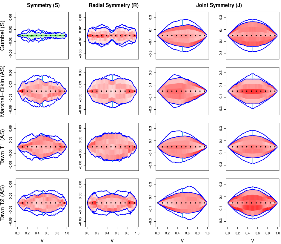
Figure 1: Functional boxplots for the visualization of copula symmetries. The parameter(s) of each copula is chosen to make its Kendall’s tau equal/close to $0.5$. Especially, the Marshall-Olkin copula takes the parameters $(0.55,0.85)$, and the Tawn copula, regardless of its types, takes the parameters $(4.28,0.60)$. The corresponding test functions are constructed with $n=1000,m=250$ and $p=100$, and the values of $v_{j},w_{j}$ for all $j\in\{1,\ldots,m\}$ are randomly chosen from the unit interval $[0,1]$. Note that the plots of copulas that inherit the specified symmetries are featured by green-centered regions, whereas those who disobey the structures are featured by red ones.

2.4 Rank-based hypothesis testing procedure

In Section 2.3, we explored the visualization of copula structures present in a given sample or dataset. We discussed the relevant asymptotic results and demonstrated how functional boxplots of selected test functions can provide intuitive indications of various symmetries. To thoroughly investigate and quantify these symmetries, we introduce a one-sample ranked-based hypothesis testing procedure. This procedure is a modification of the methods proposed by Huang and Sun (2019) and Huang et al. (2023) for testing the separability and symmetry of univariate and multivariate covariance functions. Our adapted approach allows us to assess the presence of symmetries in copula structures in a robust and statistically rigorous manner. Both of these methods can be considered as adaptations of the two-sample rank-based test proposed by López-Pintado and Romo (2009). The original test is designed to determine whether two sets of functional data are derived from the same distribution. In a similar manner, we modify this test to examine reflection symmetry as the initial step. Subsequently, by making specific adjustments, the procedure can be extended to test radial and joint symmetry.

Suppose that we have the observations $\bm{U}_{i}$’s or the pseudo-observations $\widehat{\bm{U}}_{i}$’s for $i=1,\ldots,n$. As expected, for $v\in[0,1]$ the null $\mathcal{H}_{0}$ and the alternative $\mathcal{H}_{a}$ are

• $f^{{}^{S}}_{v}=g^{{}^{S}}_{v}=0\leavevmode\nobreak\$;

• $f^{{}^{S}}_{v}=g^{{}^{S}}_{v}\neq 0$.

The details of the procedure are demonstrated as follows:

1. Estimate the values of the reflection symmetry test functions $\widehat{f}^{{}^{\hskip 1.42262ptS}}_{v_{1}},\ldots,\widehat{f}^{{}^{\hskip 1.42262ptS}}_{v_{m}},\widehat{g}^{{}^{\hskip 1.13809ptS}}_{w_{1}},\ldots,\widehat{g}^{{}^{\hskip 1.13809ptS}}_{w_{m}}$ over the evenly spaced points $\{0\leq t_{1},\ldots,t_{p}\leq 1\}$ as in Table 1 by $\bm{U}_{i}$’s, or $\widehat{\bm{U}}_{i}$’s, where for any $j\in\{1,\ldots,m\}$, $v_{j}$ and $w_{j}$ are randomly generated from the unit interval $[0,1]$.

2. Simulate from a reflection symmetric copula to obtain a set of $n$ observations, $\bm{V}^{{}^{\mathcal{H}_{0}}}_{i},\hskip 2.84526pti\in\{1,\ldots,n\}$. Further details on how to simulate the observations $\bm{V}^{{}^{\mathcal{H}_{0}}}_{i}$ are described in Section 2.4.1.

3. Estimate the values of the reflection symmetry test functions $\widehat{f}^{{}^{\hskip 2.84526pt\mathcal{H}_{0}}}_{v_{1}},\ldots,\widehat{f}^{{}^{\hskip 2.84526pt\mathcal{H}_{0}}}_{v_{m_{0}}},\widehat{g}^{{}^{\hskip 2.84526pt\mathcal{H}_{0}}}_{w_{1}},\ldots,\widehat{g}^{{}^{\hskip 2.84526pt\mathcal{H}_{0}}}_{w_{m_{0}}}$ over the evenly spaced points $\{0\leq t_{1},\ldots,t_{p}\leq 1\}$ as in Table 1 by $\bm{V}^{\mathcal{H}_{0}}_{i}$’s, where for any $j^{0}\in\{1,\ldots,m_{0}\}$, $v_{j^{0}}$ and $w_{j^{0}}$ are randomly generated from the unit interval $[0,1]$.

4. Combine the values of $\widehat{f}^{{}^{\hskip 1.42262ptS}}_{v_{1}},\ldots,\widehat{f}^{{}^{\hskip 1.42262ptS}}_{v_{m}},\widehat{g}^{{}^{\hskip 1.13809ptS}}_{w_{1}},\ldots,\widehat{g}^{{}^{\hskip 1.13809ptS}}_{w_{m}}$ with those of $\widehat{f}^{{}^{\hskip 2.84526pt\mathcal{H}_{0}}}_{v_{1}},\ldots,\widehat{f}^{{}^{\hskip 2.84526pt\mathcal{H}_{0}}}_{v_{m_{0}}},\widehat{g}^{{}^{\hskip 2.84526pt\mathcal{H}_{0}}}_{w_{1}},\ldots,\widehat{g}^{{}^{\hskip 2.84526pt\mathcal{H}_{0}}}_{w_{m_{0}}}$ to form a discretized functional data set of size $2(m+m_{0})$. Compute their modified band depths (see e.g., López-Pintado and Romo, 2009; Sun et al., 2012).

5. Rank the $2(m+m_{0})$ test functions according to their depth values. In case of any ties, we assign distinct ordinal numbers at random to the test functions that compare equal in terms of the depth values. Suppose that $\widehat{f}^{{}^{\hskip 1.42262ptS}}_{v_{1}},\ldots,\widehat{f}^{{}^{\hskip 1.42262ptS}}_{v_{m}},\widehat{g}^{{}^{\hskip 1.13809ptS}}_{w_{1}},\ldots,\widehat{g}^{{}^{\hskip 1.13809ptS}}_{w_{m}}$ are associated with the ranks $r_{1},\ldots,r_{2m_{0}}$. Define the test statistic $W=\sum_{i=1}^{2m_{0}}r_{i}$.

The null hypothesis $\mathcal{H}_{0}$ is rejected when $W$ is significantly small because it means that the test functions $\widehat{f}^{{}^{\hskip 1.42262ptS}}_{v_{1}},\ldots,\widehat{f}^{{}^{\hskip 1.42262ptS}}_{v_{m}},\widehat{g}^{{}^{\hskip 1.13809ptS}}_{w_{1}},\ldots,\widehat{g}^{{}^{\hskip 1.13809ptS}}_{w_{m}}$ are more deviated from zero. The definition of the test statistic $W$ here takes the essence of the Wilcoxon, or equivalently Mann-Whitney, test statistic. Hence, one can also deem the proposed hypothesis testing as a modification of the two-sample Wilcoxon rank-sum test for one functional data set. The null distribution of $W$ is estimated by $N_{b}$ bootstrap samples of size $n$. More specifically, we generate $N_{b}$ samples from the reflection symmetry copula in Step 2. For the $b$-th sample, $b\in\{1,\ldots,N_{b}\}$, we regard it as a set of $\bm{U}_{i}$’s and follow the above procedure to calculate the corresponding test statistic $W_{b}$. Eventually, the null distribution of $W$ is approximated by all of these test statistics: $W_{1},\ldots,W_{N_{b}}$. For the details on how to carry out such a one-sample bootstrapping method in hypothesis testing, we refer to Section 16.4 in Efron and Tibshirani (1993).

Some features of the procedure are worth further discussion. First, the number of observations simulated from a reflection symmetry copula needs to be the same as the original sample size $n$. Otherwise, even if the test functions $\widehat{f}^{{}^{\hskip 1.42262ptS}}_{v_{1}},\ldots,\widehat{f}^{{}^{\hskip 1.42262ptS}}_{v_{m}},\widehat{g}^{{}^{\hskip 1.13809ptS}}_{w_{1}},\ldots,\widehat{g}^{{}^{\hskip 1.13809ptS}}_{w_{m}}$ came from a reflection symmetry copula, they would still be more centered/deviated with respect to zero, thereby having greater depth values, compared to $\widehat{f}^{{}^{\hskip 2.84526pt\mathcal{H}_{0}}}_{v_{1}},\ldots,\widehat{f}^{{}^{\hskip 2.84526pt\mathcal{H}_{0}}}_{v_{m_{0}}},\widehat{g}^{{}^{\hskip 2.84526pt\mathcal{H}_{0}}}_{w_{1}},\ldots,\widehat{g}^{{}^{\hskip 2.84526pt\mathcal{H}_{0}}}_{w_{m_{0}}}$. This is because larger or smaller sample sizes make empirical copulas better or worse approximations of the underlying true copulas.

Second, the values of $p$, $m$, and $m_{0}$ in Steps 1 and 3 are hyperparameters that one can tune at will. Nonetheless, it is observed that setting $p=100$ is sufficient, while $m$ and $m_{0}$ have better to be large to guarantee the ideal empirical size and power of the test. Particularly, we notice that having $m$ and $m_{0}$ greater than $n$ yields better performances. Once both $m$ and $m_{0}$ satisfy the property, their values tend to have little effect on its performance.

Third, the most notable difference between our procedure and those used in López-Pintado and Romo (2009), Huang and Sun (2019) and Huang et al. (2023) lies in the absence of a reference data set. The ideas in their approaches originate with the hypothesis testing procedure designed by Liu and Singh (1993) that performs the detection of (dis)similarity in two multivariate distributions using quality index. Particularly, they introduced the treatment with a reference data set to identify the change in population locations. In the context of functional data, it describes the scenario when the two samples of functional curves appear to form two separated bands, each of which comprises only curves from one group as shown in Figure 2. However, it should not be a concern in our testing procedure thanks to the introduction of $\widehat{g}^{{}^{\hskip 1.13809ptS}}_{w_{1}},\ldots,\widehat{g}^{{}^{\hskip 1.13809ptS}}_{w_{m}}$ which are rough reflections of the test functions $\widehat{f}^{{}^{\hskip 1.13809ptS}}_{v_{1}},\ldots,\widehat{f}^{{}^{\hskip 1.13809ptS}}_{v_{m}}$ with respect to zero. As one may see later, we actually generate the observations $\bm{V}^{\mathcal{H}_{0}}_{i},i\in\{1,\ldots,n\}$ from a mixture ($M$) of empirical copulas in Step 2 under the assumption that $M$ is close to a truly reflection symmetry copula. Then, if we had to simulate a reference data set, the empirical copula of the reference data set might be more symmetric than that of the observations $\bm{V}^{\mathcal{H}_{0}}_{i},i\in\{1,\ldots,n\}$ when the sample size $n$ is not sufficiently large. This could lead to a not-so-small test statistic in the approach of Huang and Sun (2019) or Huang et al. (2023) as the test functions constructed from the reference data set might tend to be slightly more centered around zero. Certainly, the absence of a reference data set also saves memory storage.

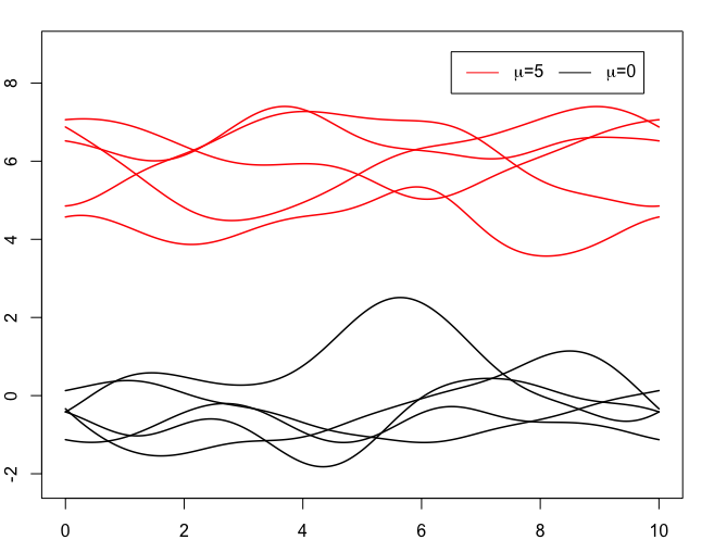
Figure 2: In the context of functional data, the approach of Liu and Singh (1993) can be interpreted as the scenario where two samples of functional curves exhibit a distinct pattern. Specifically, the curves from each group form separate bands, with little to no overlap between the two groups.

2.4.1 Simulation under $\mathcal{H}_{0}$

Lastly, it is important to address the choice of the reflection symmetric copula in Step 2 and explain how to simulate from it. In order to maintain the nonparametric nature of the procedure, it is crucial to avoid selecting any parametric copula. In lieu, we propose to construct the estimated reflection symmetric copula $\widehat{C}^{S}$ given, for all $(u,v)$, by either

$$\widehat{C}^{S}(u,v)=\frac{1}{2}\Big{(}\widehat{C}_{n}(u,v)+\widehat{C}_{n}(v,u)\Big{)}$$

or

$$\widehat{C}^{S}(u,v)=\frac{1}{2}\Big{(}\widehat{D}_{n}(u,v)+\widehat{D}_{n}(v,u)\Big{)},$$

depending on the types of data set we have.

Proposition 4.

Given any bivariate copula $C$, the copula $\tilde{C}$ defined, for all $(u,v)\in[0,1]^{2}$, by

$$\tilde{C}(u,v)=\frac{1}{2}\Big{(}C(u,v)+C(v,u)\Big{)}$$

is a reflection symmetric copula.

We prove this result in the Appendix A.4.

As a mixture of two empirical copulas, one should have no difficulty simulating from $\widehat{C}^{S}$. Note that $\widehat{C}^{S}$ is not really a copula itself, but it serves as an appropriate estimation of the reflection symmetric copula $\tilde{C}$ (Rüschendorf, 1976). Apart from the intuition suggested by Proposition 4, Figure 3 provides a visual assurance for the simulation method.

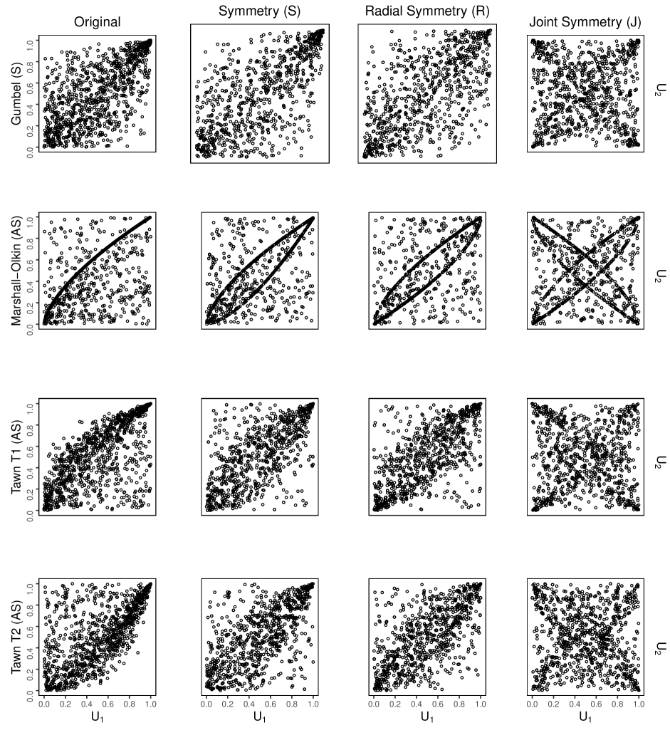
Figure 3: Rank plots for the different copula models considered in Section 2.3

By closely following the aforementioned procedure and making appropriate adjustments, one can conduct tests for radial and joint symmetries. Specifically, in Step 2, a copula that exhibits radial or joint symmetry needs to be constructed. Table 2 provides a summary of the proposed estimated copulas for this purpose, and the following Propositions provide justification for these choices. To ensure clarity in our notation, we denote the survival copula of any copula $C$ as $C^{\ast}$. Proofs of the Propositions 5 and 6 can be found in the Appendices A.5 and A.6, respectively.

Proposition 5.

Given any bivariate copula $C$, the copula $\tilde{C}$ defined, for all $(u,v)\in[0,1]^{2}$, by

$$\tilde{C}(u,v)=\frac{1}{2}\Big{(}C(u,v)+C^{\ast}(u,v)\Big{)}$$

is a radially symmetric copula.

Proposition 6.

Given any copula $C$, the copula $\tilde{C}$ defined, for all $(u,v)\in[0,1]^{2}$, by

$$\tilde{C}(u,v)=\frac{1}{4}\Big{(}C(u,v)+u-C(u,1-v)+v-C(1-u,v)+C^{\ast}(u,v)\Big{)}$$

is a jointly symmetric copula.

Type	Access	Simulated Distribution
S	$(U_{1},U_{2})$	$\widehat{C}^{S}(u,v)=\frac{1}{2}\Big{(}\widehat{C}_{n}(u,v)+\widehat{C}_{n}(v,u)\Big{)}$
	$(X_{1},X_{2})$	$\widehat{C}^{S}(u,v)=\frac{1}{2}\Big{(}\widehat{D}_{n}(u,v)+\widehat{D}_{n}(v,u)\Big{)}$
R	$(U_{1},U_{2})$	$\widehat{C}^{R}(u,v)=\frac{1}{2}\Big{(}\widehat{C}_{n}(u,v)+\widehat{C}^{\ast}_{n}(u,v)\Big{)}$
	$(X_{1},X_{2})$	$\widehat{C}^{R}(u,v)=\frac{1}{2}\Big{(}\widehat{D}_{n}(u,v)+\widehat{D}^{\ast}_{n}(u,v)\Big{)}$
J	$(U_{1},U_{2})$	$\widehat{C}^{{J}}(u,v)=\hskip 2.84526pt\tfrac{1}{4}\Big{(}\widehat{C}_{n}(u,v)+u-\widehat{C}_{n}(u,1-v)+v-\widehat{C}_{n}(1-u,v)+\widehat{C}^{\ast}_{n}(u,v)\Big{)}$
	$(X_{1},X_{2})$	$\widehat{C}^{{J}}(u,v)=\hskip 2.84526pt\tfrac{1}{4}\Big{(}\widehat{D}_{n}(u,v)+u-\widehat{D}_{n}(u,1-v)+v-\widehat{D}_{n}(1-u,v)+\widehat{D}^{\ast}_{n}(u,v)\Big{)}$

Table 2: Definitions of estimated copulas constructed to test different types of symmetry. $\widehat{C}^{\ast}_{n}$ and $\widehat{D}^{\ast}_{n}$ denote the estimator for the survival copulas associated with the underlying copula.

3 Simulation Study

We performed simulations to evaluate the effectiveness of our testing procedures for the three copula structures described in Section 2.1. In each simulation, we estimated 1200 test functions, and the tests were conducted at a nominal level of $5\%$. We utilized $N_{b}=1000$ bootstrap samples for our analysis. To assess the performance of our approach for testing reflection symmetry, we compared it to the tests proposed by Genest et al. (2012) and Li and Genton (2013). The results, including the sizes and powers of the test for reflection symmetry, are summarized in Table 3. To evaluate the power of our tests, we introduce asymmetry to the copula models using Khoudraji’s device (Khoudraji, 1995). Specifically, we used an asymmetric version of a copula $C(u,v)$, defined for $(u,v)\in[0,1]^{2}$, given by:

$$K_{\delta}(u,v)=u^{\delta}C(u^{1-\delta},v),$$

where $\delta\in(0,1)$. Previous studies (Genest et al., 2012) have shown that Khoudraji’s device introduces minimal asymmetry when Kendall’s $\tau\leq 0.5$. The maximum level of asymmetry is typically observed around $\delta=0.5$. The R codes for implementing the visualization and hypotheses testing procedures are available at https://github.com/cfjimenezv07/Visualization-and-Assessment-of-Copula-Symmetry.

			Clayton				Gaussian				Gumbel
			$n$				$n$				$n$
$\delta$	$\tau$		100	250	500	1000	100	250	500	1000	100	250	500	1000
0	1/4	E Z I S	0.044	0.048	0.059	0.062	0.053	0.052	0.046	0.066	0.050	0.063	0.059	0.063
	1/2		0.021	0.043	0.051	0.053	0.031	0.039	0.048	0.064	0.038	0.044	0.055	0.053
	3/4		0.007	0.002	0.007	0.007	0.001	0.002	0.003	0.004	0.007	0.008	0.009	0.019
0	$0^{\ast}$		0.045	0.060	0.059	0.060
1/4	0.5	R E W O P	0.121	0.297	0.547	0.796	0.089	0.267	0.552	0.850	0.119	0.312	0.609	0.903
	0.7		0.374	0.814	0.981	0.999	0.336	0.860	0.995	1.000	0.365	0.886	0.994	1.000
	0.9		0.675	0.977	0.996	1.000	0.740	0.987	0.998	1.000	0.728	0.990	1.000	1.000
1/2	0.5		0.149	0.358	0.630	0.872	0.187	0.511	0.826	0.990	0.264	0.690	0.929	0.998
	0.7		0.483	0.926	0.998	1.000	0.664	0.986	1.000	1.000	0.736	0.992	1.000	1.000
	0.9		0.908	1.000	1.000	1.000	0.951	1.000	1.000	1.000	0.940	1.000	1.000	1.000
3/4	0.5		0.087	0.210	0.334	0.557	0.178	0.450	0.743	0.959	0.301	0.656	0.930	0.995
	0.7		0.254	0.629	0.897	0.996	0.500	0.929	0.999	1.000	0.605	0.957	0.998	1.000
	0.9		0.662	0.984	1.000	1.000	0.761	0.999	1.000	1.000	0.768	0.985	1.000	1.000

Table 3: Empirical sizes and powers of the test of symmetry in the setting as Genest et al. (2012) and Li and Genton (2013). The sizes for the independent copula are $\delta=\tau=0$.

Our results indicate that under small and moderate $\tau$, the sizes converge to the nominal value as the sample size increases, but with larger $\tau$, the sizes are somewhat below the nominal level. The powers of the tests increase as the sample size increases. When comparing our results to Table 3 in Genest et al. (2012), their approach generally achieves better powers for a small sample size of $n=250$. In contrast, our approach demonstrates significantly improved powers as the sample size increases. This is expected as our rank-based test relies on the asymptotic distribution of the test functions and the empirical copula process.

When comparing our simulation results to Table 1 in Li and Genton (2013), we find that our results align with most of the reported powers and sizes. However, our approach achieves considerably higher powers even at smaller sample sizes, particularly for intermediate values of $\tau$ where the maximum asymmetry is expected.

For the tests of radial and joint symmetry, we selected five commonly used copulas. The sizes and powers of both testing procedures are presented in Table 4. To evaluate the performance of our approach in testing radial symmetry, we compared it to the methods proposed by Li and Genton (2013) and Genest and Nešlehová (2014). Additionally, we compared our approach for testing joint symmetry to the methods reported by Li and Genton (2013).

		Radial					Joint
	$\tau$	$n=$	$100$	$250$	$500$	$1000$	$n=$	$100$	$250$	$500$	$1000$
$\Pi$	$0$	E Z I S	0.060	0.073	0.065	0.060	SIZE	0.030	0.029	0.024	0.048
Frank	1/4		0.054	0.060	0.059	0.054	R E W O P	0.685	0.963	0.997	1.000
	1/2		0.050	0.064	0.058	0.059		0.968	1.000	1.000	1.000
	3/4		0.016	0.041	0.037	0.046		0.975	0.999	1.000	1.000
Gaussian	1/4		0.062	0.060	0.047	0.059		0.725	0.984	1.000	1.000
	1/2		0.041	0.041	0.054	0.054		0.976	0.999	1.000	1.000
	3/4		0.009	0.022	0.014	0.031		0.973	1.000	1.000	1.000
Clayton	1/4	R E W O P	0.228	0.491	0.830	0.985		0.706	0.957	0.999	1.000
	1/2		0.516	0.833	0.985	1.000		0.966	0.999	1.000	1.000
	3/4		0.291	0.512	0.912	0.996		0.976	1.000	1.000	1.000
Gumbel	1/4		0.110	0.333	0.510	0.695		0.696	0.974	0.998	1.000
	1/2		0.166	0.486	0.723	0.909		0.974	1.000	1.000	1.000
	3/4		0.042	0.322	0.580	0.815		0.978	0.999	1.000	1.000

Table 4: Sizes and powers of the test of radial and joint symmetry in the setting as Li and Genton (2013) and Genest and Nešlehová (2014). One bootstrap sample is used to estimate the distribution of the test statistic $W$ under the null.

The sizes of both tests closely align with the nominal level of $5\%$ for values of $\tau$ equal to $1/4$ and $1/2$. However, for larger values of $\tau$, the sizes are achieved at larger sample sizes. Specifically, in the case of the radial symmetry test, our results are consistent with those presented in Table 2 of Li and Genton (2013), and once again our testing approach achieves the nominal levels at smaller sample sizes.

In comparison to the results presented in Table 1 of Genest and Nešlehová (2014) for the Frank and Gaussian copula models they considered, our approach achieves sizes that are closer to the nominal level. Although their performance improves for larger sample sizes, our approach outperforms them even in scenarios with larger sample sizes.

Regarding the joint symmetry copula structure, our achieved powers are significantly higher compared to the powers obtained for the radial symmetry property, similar results are presented in Table 2 of Li and Genton (2013).

4 Data Applications

To illustrate the procedures herein, we apply our visualization and hypothesis testing methodology to two real-world data sets. The Nutritional Habits Survey Data is in Section 4.1, and the wind speed dataset in Saudi Arabia is in Section 4.2.

4.1 Nutritional Habits Survey Data

The dataset used here comes from a survey conducted by the U.S. Department of Agriculture in 1985. The survey aimed to investigate the dietary habits of 737 women aged between 25 and 50 years. Specifically, the survey collected daily intake measurements of five variables: calcium (mg), iron (mg), protein (g), vitamin A (mg), and vitamin C (mg).

In previous analyses, Genest et al. (2012) employed a Cramér-von Mises statistic to evaluate the bivariate reflection symmetry of the pairwise copulas. Similarly, Li and Genton (2013) utilized a nonparametric method based on the asymptotic distribution of the empirical copula process to assess reflection symmetry for this dataset. In our study, we conducted a test using our rank-based method and obtained corresponding p-values, which are presented in the top-right corner of each subplot in Figure 4.

The pattern of p-values obtained in our study exhibits similarities to the findings reported by Genest et al. (2012) and Li and Genton (2013), leading to similar conclusions for some pairs. However, there are notable differences. Unlike Genest et al. (2012), our test does not reject the reflection symmetry copula at a $5\%$ significance level for the pairs (iron, vitamin A), (iron, vitamin C), and (protein, vitamin A). Conversely, we do reject the reflection symmetry copula for the pair (protein, vitamin C).

When comparing our results to those of Li and Genton (2013), we find much closer agreement. The only difference in conclusions arises for the two pairs: (protein, vitamin C), where we reject the reflection symmetry copula, and (iron, vitamin A), where we do not reject it. Notably, the pair (iron, vitamin A) differs from the conclusions of both Genest et al. (2012) and Li and Genton (2013). However, our proposed visualization method reveals that the majority of the test functions exhibit high density around the zero level for this pair.

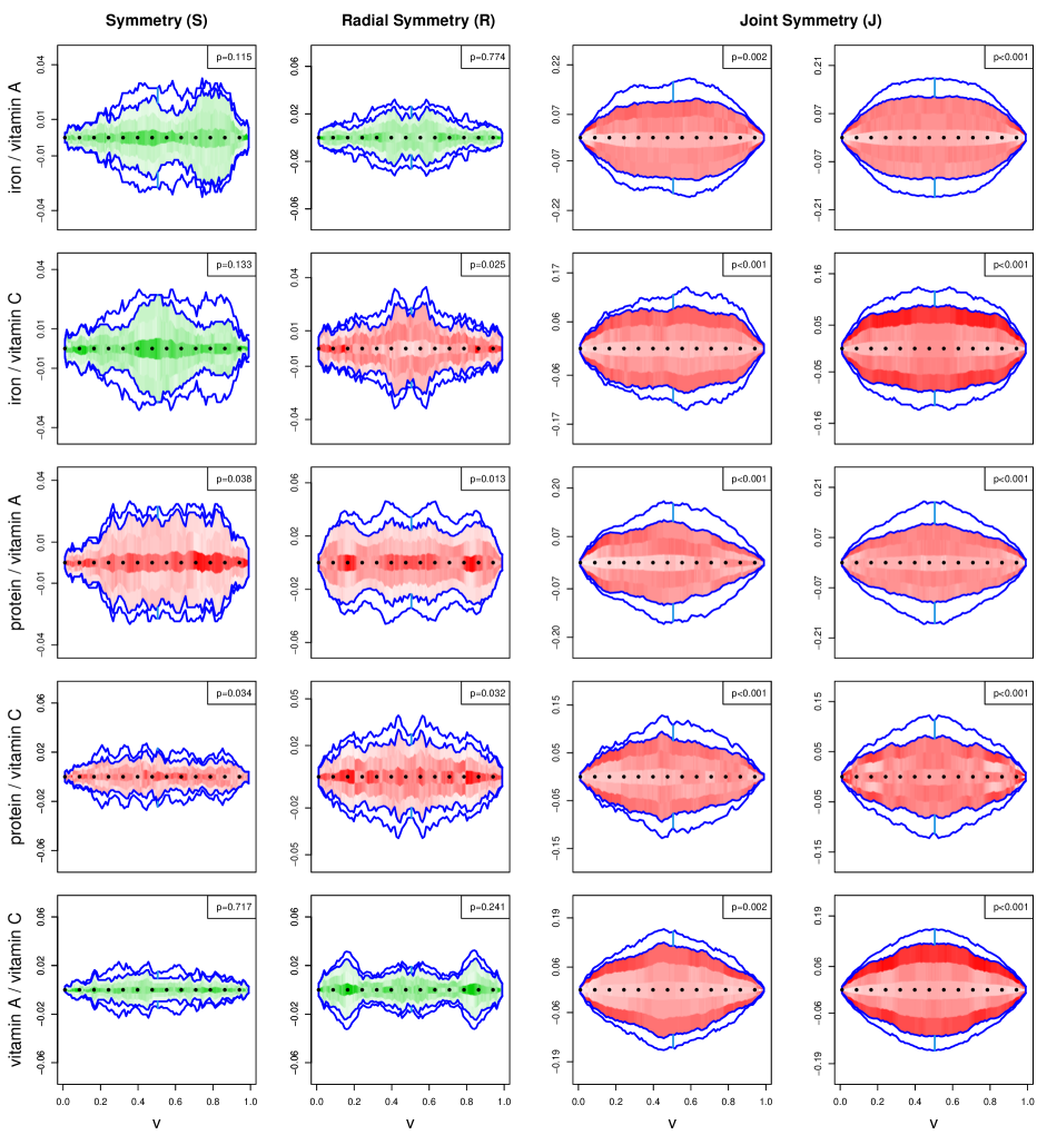
Figure 4: Visualizations and testing results for copula symmetries over the $5$ random variables in the nutritional data set.

4.2 Wind data

In this study, we analyze a trivariate wind speed dataset obtained from Yip (2018). The dataset comprises bi-weekly mid-day wind speed measurements recorded over the period of 2009-2014 at three specific locations near Dumat Al Jandal, the site of the first wind farm currently under construction in Saudi Arabia. The dataset consists of $n=156$ trivariate wind speed vectors, each containing measurements from three positions.

Understanding the dependence structure within these trivariate wind speed vectors is crucial for assessing how wind patterns impact the electricity generation of the nearby wind farm. By analyzing this dependence structure, we can gain insights into the interactions between wind speeds at different locations and optimize the operation and output of the wind farm.

One specific aspect of interest is evaluating whether a potential copula model, which quantifies the dependence among bivariate positions, exhibits a specific symmetry structure. This assessment allows us to examine the symmetry properties of a potential copula model and determine if it aligns with the desired symmetry structure. Understanding the symmetry properties can be essential for accurately modeling and predicting wind speed behavior.

Figure 5 presents the visualization and hypothesis testing results for the dataset under consideration, focusing on the three copula structures analyzed in the paper. The results show that joint symmetry is rejected for all pairs of locations. However, reflection symmetry and radial symmetry are not rejected by the bivariate dataset formed by positions 2 and 3. This is indicated by the functional boxplot, which demonstrates functions distributed widely around zero and the corresponding large p-values. In summary, our approach suggests using asymmetric copula models to properly capture the dependence in these wind speed data.

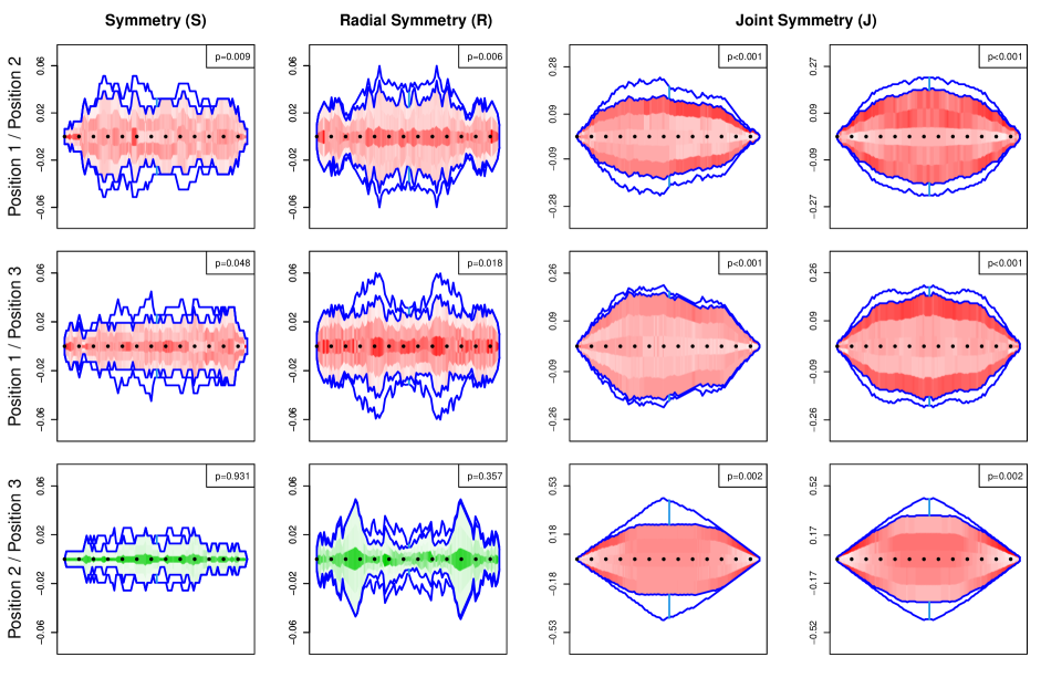
Figure 5: Visualizations and testing results for copula symmetries over the $3$ locations for the wind data in Saudi Arabia.

5 Discussion

In this paper, we have presented a comprehensive framework for visualizing and testing common assumptions regarding copula structures, such as reflection symmetry, radial symmetry, and joint symmetry. Our approach utilizes functional data analysis techniques to construct test functions based on bivariate copulas at specific discrete points. These test functions effectively summarize the copula structures and provide valuable insights into their adherence to specific structures.

To visually represent the copula structures, we employ functional boxplots, which depict the functional median and variability of the test functions. These visualizations allow us to assess the departure from zero and gain insights into the degree to which the copula structures conform to the desired assumptions.

Additionally, we have introduced a nonparametric testing procedure to evaluate the significance of deviations from symmetry. Through extensive simulation studies involving various copula models, we have demonstrated the reliability and power of our method, particularly for moderate to large sample sizes. The numerical experiments and data analyses conducted in this study have consistently shown robust testing results across different datasets, and the visualization technique has proven useful in extracting preliminary information directly from the data. It is worth mentioning that our functional data approach can be extended to test copula properties beyond symmetry as well.

It is important to note that our testing method relies on the asymptotic distribution of the estimators of the test functions, which are derived from empirical copula processes. As a result, the small sample properties of our test may not be as optimal as certain existing testing methods. The required sample size for our testing approach can vary depending on the specific copula structure under examination, but in general, larger sample sizes tend to enhance the size and power of the test. Thus, increasing the sample size is recommended to improve the overall performance of the test in terms of accuracy and sensitivity.

Finally, our visualization and testing techniques were applied to two real-world datasets: a nutritional habits survey with five variables and wind speed data from three locations in Saudi Arabia. These applications provided valuable insights into the underlying structures and patterns within the datasets, demonstrating the effectiveness of our approach in gaining a better understanding of the data.

Appendix A Appendix

A.1 Proof of Proposition 1

The proof of the proposition is essentially the same as that of Proposition 2 in Genest et al. (2012). They focus on the asymptotic results when the underlying copula $C$ is indeed reflection symmetric. We firstly consider the case when $\widehat{f}^{{}^{\hskip 1.42262ptS}}_{v}(t)=\widehat{C}_{n}(t,v)-\widehat{C}_{n}(v,t)$. The map

$$\mathcal{T}^{S}_{v}:\ell([0,1]^{2})\rightarrow\ell([0,1]):f\mapsto\big{(}t\mapsto f(t,v)-f(v,t)\big{)}\\$$

is a continuous function. Thus, the Continuous Mapping Theorem (van der Vaart and Wellner (1996), Theorem 1.3.6) and result (5) imply that $\sqrt{n}\left\{\widehat{f}^{{}^{\hskip 1.42262ptS}}_{v}(t)-f^{{}^{S}}_{v}(t)\right\}\xrightarrow[\hskip 14.22636pt]{d}\mathbb{E}^{{}^{S}}_{v}(t):=\mathbb{C}(t,v)-\mathbb{C}(v,t)$ for all $t\in[0,1]$, where $\mathbb{E}^{{}^{S}}_{v}$ is a centered Gaussian random field with covariance function given at each $s,t\in[0,1]$ by

$$\mathrm{Cov}\{\mathbb{E}^{{}^{S}}_{v}(t),\hskip 2.84526pt\mathbb{E}^{{}^{S}}_{v}(s)\}= \hskip 5.69054pt\mathrm{Cov}\{\mathbb{C}(t,v)-\mathbb{C}(v,t),\hskip 2.84526pt\mathbb{C}(s,v)-\mathbb{C}(v,s)\}$$

$$= \hskip 5.69054ptC(t\land s,v)-C(t,v)C(s,v)+C(v,t\land s)-C(v,t)C(v,s)$$

$$-C(t\land v,s\land v)+C(t,v)C(v,s)-C(s\land v,t\land v)+C(v,t)C(s,v).$$

Similarly, if $\widehat{f}^{{}^{\hskip 1.42262ptS}}_{v}(t)=\widehat{D}_{n}(t,v)-\widehat{D}_{n}(v,t)$, we have

$$\sqrt{n}\left\{\widehat{f}^{{}^{\hskip 1.42262ptS}}_{v}(t)-f^{{}^{S}}_{v}(t)\right\}\xrightarrow[\hskip 14.22636pt]{d}\widehat{\mathbb{E}}^{{}^{S}}_{v}(t):= \hskip 5.69054pt\mathbb{C}(t,v)-\dot{C}_{1}(t,v)\mathbb{C}(t,1)-\dot{C}_{2}(t,v)\mathbb{C}(1,v)$$

$$-\mathbb{C}(v,t)+\dot{C}_{1}(v,t)\mathbb{C}(v,1)+\dot{C}_{2}(v,t)\mathbb{C}(1,t)$$

for all $t\in[0,1]$, where $\widehat{\mathbb{E}}^{{}^{S}}_{v}$ is a centered Gaussian random field. One can easily derive its covariance function, but the expression is omitted here in view of its intricate closed form.

A.2 Proof of Proposition 2

We first consider the case when $\widehat{f}^{{}^{\hskip 1.42262ptR}}_{v}(t)=\widehat{C}_{n}(t,v)-\widehat{C}_{n}(1-t,1-v)+1-t-v$. Notice that

$$\sqrt{n}\left\{\widehat{f}^{{}^{\hskip 1.42262ptR}}_{v}(t)-f^{{}^{R}}_{v}(t)\right\} =\sqrt{n}\left\{\widehat{C}_{n}(t,v)-\widehat{C}_{n}(1-t,1-v)-\big{(}C(t,v)-C(1-t,1-v)\big{)}\right\}$$

$$=\sqrt{n}\left\{\widehat{C}_{n}(t,v)-C(t,v)\right\}-\sqrt{n}\left\{\widehat{C}_{n}(1-t,1-v)-C(1-t,1-v)\right\}$$

$$=\mathbb{C}_{n}(t,v)-\mathbb{C}_{n}(1-t,1-v).$$

Since the map

$$\mathcal{T}^{R}_{v}:\ell([0,1]^{2})\rightarrow\ell([0,1]):f\mapsto\big{(}t\mapsto f(t,v)-f(1-t,1-v)\big{)}\\$$

is a continuous functional, the Continuous Mapping Theorem and result (5) imply that $\sqrt{n}\left\{\widehat{f}^{{}^{\hskip 1.42262ptR}}_{v}(t)-f^{{}^{R}}_{v}(t)\right\}$ $\xrightarrow[\hskip 14.22636pt]{d}\mathbb{E}^{{}^{R}}_{v}(t):=\mathbb{C}(t,v)-\mathbb{C}(1-t,1-v)$ for all $t\in[0,1]$, where $\mathbb{E}^{{}^{R}}_{v}$ is a centered Gaussian random field with covariance function given at each $s,t\in[0,1]$ by

$$\mathrm{Cov}\{ \mathbb{E}^{{}^{R}}_{v}(t),\hskip 2.84526pt\mathbb{E}^{{}^{R}}_{v}(s)\}$$

$$= \hskip 5.69054pt\mathrm{Cov}\{\mathbb{C}(t,v)-\mathbb{C}(1-t,1-v),\hskip 2.84526pt\mathbb{C}(s,v)-\mathbb{C}(1-s,1-v)\}$$

$$= \hskip 5.69054ptC(t\land s,v)-C(t,v)C(s,v)+C(1-t\lor s,1-v)-C(1-t,1-v)C(1-s,1-v)$$

$$-C(t\land(1-s),v\land(1-v))+C(t,v)C(1-s,1-v)$$

$$-C((1-t)\land s,v\land(1-v))+C(s,v)C(1-t,1-v),$$

where for all $a,b\in\mathbb{R}$, $a\lor b=\max\{a,b\}$. Similarly, if $\widehat{f}^{{}^{\hskip 1.42262ptR}}_{v}(t)=\widehat{D}_{n}(t,v)-\widehat{D}_{n}(1-t,1-v)+1-t-v$, we have

$$\sqrt{n} \left\{\widehat{f}^{{}^{\hskip 1.42262ptR}}_{v}(t)-f^{{}^{R}}_{v}(t)\right\}=\mathbb{D}_{n}(t,v)-\mathbb{D}_{n}(1-t,1-v)$$

$$\xrightarrow[\hskip 14.22636pt]{d}\hskip 5.69054pt\widehat{\mathbb{E}}^{{}^{R}}_{v}(t):=\mathbb{C}(t,v)-\dot{C}_{1}(t,v)\mathbb{C}(t,1)-\dot{C}_{2}(t,v)\mathbb{C}(1,v)$$

$$\hskip 71.13188pt-\mathbb{C}(1-t,1-v)+\dot{C}_{1}(1-t,1-v)\mathbb{C}(1-t,1)+\dot{C}_{2}(1-t,1-v)\mathbb{C}(1,1-v)$$

for all $t\in[0,1]$, where $\widehat{\mathbb{E}}^{{}^{R}}_{v}$ is a centered Gaussian random field. One can derive its covariance function, but the expression is omitted here in view of its intricate closed form.

A.3 Proof of Proposition 3

The proof of this Proposition is similar to those of Propositions 1 and 2 but with a different choice of continuous functionals, and we will only present the details of the asymptotic result regarding the test function $\widehat{f}^{{}^{\hskip 1.42262ptS,1}}_{v}$. Firstly, consider the case when $\widehat{f}^{{}^{\hskip 1.42262ptS,1}}_{v}(t)=\widehat{C}_{n}(t,v)+\widehat{C}_{n}(t,1-v)-t$. Notice that

$$\sqrt{n}\left\{\widehat{f}^{{}^{\hskip 1.42262ptS,1}}_{v}(t)-f^{{}^{S,1}}_{v}(t)\right\} =\sqrt{n}\left\{\widehat{C}_{n}(t,v)+\widehat{C}_{n}(t,1-v)-\big{(}C(t,v)+C(t,1-v)\big{)}\right\}$$

$$=\sqrt{n}\left\{\widehat{C}_{n}(t,v)-C(t,v)\right\}+\sqrt{n}\left\{\widehat{C}_{n}(t,1-v)-C(t,1-v)\right\}$$

$$=\mathbb{C}_{n}(t,v)+\mathbb{C}_{n}(t,1-v).$$

Since the map

$$\mathcal{T}^{R}_{v}:\ell([0,1]^{2})\rightarrow\ell([0,1]):f\mapsto\big{(}t\mapsto f(t,v)+f(t,1-v)\big{)}\\$$

is a continuous functional, the continuous mapping theorem and result (5) imply that

$$\sqrt{n}\left\{\widehat{f}^{{}^{\hskip 1.42262ptJ,1}}_{v}(t)-f^{{}^{J,1}}_{v}(t)\right\}\xrightarrow[\hskip 14.22636pt]{d}\mathbb{E}^{{}^{J,1}}_{v}(t):=\mathbb{C}(t,v)+\mathbb{C}(t,1-v)\leavevmode\nobreak\ \forall t\in[0,1],$$

where $\mathbb{E}^{{}^{J,1}}_{v}$ is a centered Gaussian random field with covariance function given at each $s,t\in[0,1]$ by

$$\mathrm{Cov}\{ \mathbb{E}^{{}^{J,1}}_{v}(t),\hskip 2.84526pt\mathbb{E}^{{}^{J,1}}_{v}(s)\}$$

$$= \hskip 5.69054pt\mathrm{Cov}\{\mathbb{C}(t,v)+\mathbb{C}(t,1-v),\hskip 2.84526pt\mathbb{C}(s,v)+\mathbb{C}(s,1-v)\}$$

$$= \hskip 5.69054ptC(t\land s,v)+C(t,v)C(s,v)+C(t\land s,1-v)+C(t,1-v)C(s,1-v)$$

$$+C(t\land s,v\land(1-v))+C(t,v)C(s,1-v)+C(t\land s,v\land(1-v))+C(s,v)C(t,1-v),$$

where for all $a,b\in\mathbb{R}$, $a\lor b=\max\{a,b\}$. Similarly, if $\widehat{f}^{{}^{\hskip 1.42262ptS,1}}_{v}(t)=\widehat{D}_{n}(t,v)+\widehat{D}_{n}(t,1-v)-t$, we have

$$\sqrt{n} \left\{\widehat{f}^{{}^{\hskip 1.42262ptR}}_{v}(t)-f^{{}^{R}}_{v}(t)\right\}=\mathbb{D}_{n}(t,v)+\mathbb{D}_{n}(t,1-v)$$

$$\xrightarrow[\hskip 14.22636pt]{d}\hskip 5.69054pt\widehat{\mathbb{E}}^{{}^{S,1}}_{v}(t):=\mathbb{C}(t,v)-\dot{C}_{1}(t,v)\mathbb{C}(t,1)-\dot{C}_{2}(t,v)\mathbb{C}(1,v)$$

$$\hskip 71.13188pt-\mathbb{C}(1-t,1-v)+\dot{C}_{1}(1-t,1-v)\mathbb{C}(1-t,1)+\dot{C}_{2}(1-t,1-v)\mathbb{C}(1,1-v)$$

for all $t\in[0,1]$, where $\widehat{\mathbb{E}}^{{}^{S,1}}_{v}$ is a centered Gaussian random field. One can derive its covariance function, but the expression is omitted here in view of its intricate closed form.

Lemma 1.

The average of bivariate copulas is also a bivariate copula.

Proof.

Let $n\in\mathbb{N}$ be fixed, and let $C_{1},\ldots,C_{n}$ be $n$ (not necessarily mutually distinct) bivariate copulas. Define

$$\mathcal{C}(u,v)=\frac{1}{n}\sum_{i=1}^{n}C_{i}(u,v),\hskip 14.22636pt\forall(u,v)\in[0,1].$$

If $u$ or $v$ is zero, say $u=0$, we have that

$$\mathcal{C}(0,v)=\frac{1}{n}\sum_{i=1}^{n}C_{i}(0,v)=\frac{1}{n}\sum_{i=1}^{n}0=0.$$

If $u$ or $v$ is $1$, say $u=1$, one can show that

$$\mathcal{C}(1,v)=\frac{1}{n}\sum_{i=1}^{n}C_{i}(1,v)=\frac{1}{n}\sum_{i=1}^{n}v=v.$$

For any $(a_{1},a_{2}),(b_{1},b_{2})\in[0,1]^{2}$ with $a_{1}\leq b_{1}$ and $a_{2}\leq b_{2}$, we have

$$\sum_{i_{1}=0}^{1}\sum_{i_{2}=0}^{1}(-1)^{i_{1}+i_{2}}\mathcal{C}(x_{1i_{1}},x_{2i_{2}})=\sum_{i_{1}=0}^{1}\sum_{i_{2}=0}^{1}(-1)^{i_{1}+i_{2}}\Big{(}\frac{1}{n}\sum_{j=1}^{n}C_{j}(x_{1i_{1}},x_{2i_{2}})\Big{)}\\ =\frac{1}{n}\sum_{j=1}^{n}\Big{(}\sum_{i_{1}=0}^{1}\sum_{i_{2}=0}^{1}(-1)^{i_{1}+i_{2}}C_{j}(x_{1i_{1}},x_{2i_{2}})\Big{)}\geq 0,$$

where $x_{j0}=a_{j}$ and $x_{j1}=b_{j}$ for all $j\in\{1,2\}$. All of this proves that $\mathcal{C}$ is a copula. Note that the result should be easily extended to any mixture of bivariate copulas. ∎

A.4 Proof of Proposition 4

Assume that $(U,V)$ is a $C$-distributed random vector. Considering the random vector $(V,U)$, we have

$$\mathds{P}(V\leq u,U\leq v)=\mathds{P}(U\leq v,V\leq u)=C(v,u),\hskip 14.22636pt\forall(u,v)\in[0,1].$$

It follows from Sklar’s theorem that the bivariate function $\mathcal{C}$ defined, for all $(u,v)\in[0,1]$, by $\mathcal{C}(u,v)=C(v,u)$ is a copula. Thus, Proposition 4 ensures that $\tilde{C}$ is also a copula. As for the reflection symmetric structure, it is clear by the associativity of addition.

A.5 Proof of Proposition 5

Proposition 4 ensures that $\tilde{C}$ is a bivariate copula. Moreover, one can easily notice

$$\tilde{C}(u,v)-\tilde{C}(1-u,1-v)$$

$$=\frac{1}{2}\Big{(}C(u,v)+C(1-u,1-v)+u+v-1\Big{)}$$

$$\hskip 85.35826pt-\frac{1}{2}\Big{(}C(1-u,1-v)+C(u,v)+(1-u)+(1-v)-1\Big{)}$$

$$=u+v-1,$$

which tells us that $\tilde{C}$ is radially symmetric.

A.6 Proof of Proposition 6

To justify that $\tilde{C}$ is a copula, it suffices to show that the bivariate functions $C_{1}$ and $C_{2}$ given, for all $(u,v)\in[0,1]$, by

$$C_{1}(u,v)=u-C(u,1-v)\text{ \hskip 5.69054ptand\hskip 5.69054pt }C_{2}(u,v)=v-C(1-u,v)$$

are both copulas. Let $(U,V)$ be a $C$-distributed random vector. Consider the random vector $(U,1-V)$. For all $(u,v)\in[0,1]$, we have

$$\mathds{P}(U\leq u,1-V\leq v)=\mathds{P}(U\leq u,1-V\leq v)\\ =\mathds{P}(U\leq u)-\mathds{P}(U\leq u,V\leq 1-v)=u-C(u,1-v),\hskip 14.22636pt\forall(u,v)\in[0,1].$$

It follows from Sklar’s theorem that $C_{1}$ is a copula; similarly, $C_{2}$ can be shown to be the copula of $(1-u,v)$. Finally, one can check that

$$\tilde{C} (u,v)+\tilde{C}(u,1-v)$$

$$=\frac{1}{4}\Big{(}C(u,v)+u-C(u,1-v)+v-C(1-u,v)+u+v-1+C(1-u,1-v)\Big{)}$$

$$\hskip 14.22636pt+\frac{1}{4}\Big{(}C(u,1-v)+u-C(u,v)+1-v-C(1-u,1-v)$$

$$\hskip 284.52756pt+u+1-v-1+C(1-u,v)\Big{)}$$

$$=\frac{1}{4}(2u+2v-1+2u-2v+1)=u$$

and similarly verify $\tilde{C}(u,v)+\tilde{C}(1-u,v)=v$. With all of this, it can be concluded that $\tilde{C}$ is a jointly symmetric copula.

References

- Aas et al. (2009) Aas, K., C. Czado, A. Frigessi, and H. Bakken (2009). Pair-copula constructions of multiple dependence. Insurance: Mathematics and Economics 44(2), 182–198.
- Berg (2009) Berg, D. (2009). Copula goodness-of-fit testing: an overview and power comparison. The European Journal of Finance 15(7-8), 675–701.
- Bücher et al. (2011) Bücher, A., H. Dette, and S. Volgushev (2011). New estimators of the pickands dependence function and a test for extreme-value dependence. The Annals of Statistics 39(4), 1963–2006.
- Bücher et al. (2012) Bücher, A., H. Dette, and S. Volgushev (2012). A test for archimedeanity in bivariate copula models. Journal of Multivariate Analysis 110, 121–132. Special Issue on Copula Modeling and Dependence.
- Cherubini et al. (2004) Cherubini, U., E. Luciano, and W. Vecchiato (2004). Copula Methods in Finance. Wiley.
- Deheuvels (1979) Deheuvels, P. (1979). Propriétés d’existence et propriétés topologiques des fonctions de dépendance avec applications à la convergence des types pour des lois multivariées. Comptes Rendus Hebdomadaires des Séances de l’Académie des Sciences. Séries A et B 288(2), A145–A148.
- Efron and Tibshirani (1993) Efron, B. and R. J. Tibshirani (1993). An introduction to the bootstrap, Volume 57 of Monographs on Statistics and Applied Probability. Chapman and Hall, New York.
- Genest and Favre (2007) Genest, C. and A.-C. Favre (2007). Everything you always wanted to know about copula modeling but were afraid to ask. Journal of Hydrologic Engineering 12(4), 347–368.
- Genest et al. (2012) Genest, C., J. Nešlehová, and J.-F. Quessy (2012). Tests of symmetry for bivariate copulas. Annals of the Institute of Statistical Mathematics 64(4), 811–834.
- Genest and Nešlehová (2014) Genest, C. and J. G. Nešlehová (2014). On tests of radial symmetry for bivariate copulas. Statistical Papers 55(4), 1107–1119.
- Genest et al. (2009) Genest, C., B. Rémillard, and D. Beaudoin (2009). Goodness-of-fit tests for copulas: A review and a power study. Insurance: Mathematics and Economics 44(2), 199–213.
- Genest and Segers (2010) Genest, C. and J. Segers (2010). On the covariance of the asymptotic empirical copula process. Journal of Multivariate Analysis. 101(8), 1837–1845.
- Huang and Sun (2019) Huang, H. and Y. Sun (2019). Visualization and assessment of spatio-temporal covariance properties. Spatial Statistics 34, 100272, 18.
- Huang et al. (2023) Huang, H., Y. Sun, and M. G. Genton (2023). Test and visualization of covariance properties for multivariate spatio-temporal random fields. Journal of Computational and Graphical Statistics 32, 1545–1555.
- Jaser and Min (2021) Jaser, M. and A. Min (2021). On tests for symmetry and radial symmetry of bivariate copulas towards testing for ellipticity. Computational Statistics 36(3), 1–26.
- Jaworski (2010) Jaworski, P. (2010). Testing archimedeanity. In C. Borgelt, G. González-Rodríguez, W. Trutschnig, M. A. Lubiano, M. Á. Gil, P. Grzegorzewski, and O. Hryniewicz (Eds.), Combining Soft Computing and Statistical Methods in Data Analysis, Berlin, Heidelberg, pp. 353–360. Springer Berlin Heidelberg.
- Joe (2014) Joe, H. (2014). Dependence Modeling with Copulas. Chapman and Hall/CRC.
- Khoudraji (1995) Khoudraji, A. (1995). Contributions à l’étude des copules et à la modélisation de valeurs extrêmes bivariées. Ph. D. thesis, National Library of Canada = Bibliothèque nationale du Canada Ottawa.
- Li and Genton (2013) Li, B. and M. G. Genton (2013). Nonparametric identification of copula structures. Journal of the American Statistical Association. 108(502), 666–675.
- Liu and Singh (1993) Liu, R. Y. and K. Singh (1993). A quality index based on data depth and multivariate rank tests. Journal of the American Statistical Association. 88(421), 252–260.
- López-Pintado and Romo (2009) López-Pintado, S. and J. Romo (2009). On the concept of depth for functional data. Journal of the American Statistical Association 104(486), 718–734.
- Mikosch (2006) Mikosch, T. (2006). Copulas: Tales and facts—rejoinder. Extremes 9(1), 55–62.
- Nelsen (1993) Nelsen, R. B. (1993). Some concepts of bivariate symmetry. Journal of Nonparametric Statistics. 3(1), 95–101.
- Nelsen (2006) Nelsen, R. B. (2006). An Introduction to Copulas. Springer.
- Patton (2006) Patton, A. J. (2006). Modelling asymmetric exchange rate dependence. International Economic Review 47(2), 527–556.
- Patton (2012) Patton, A. J. (2012). Copula-based models for financial time series. In T. G. Andersen, R. A. Davis, J.-P. Kreiß, and T. Mikosch (Eds.), Handbook of Financial Time Series, pp. 767–785. Springer.
- Quessy (2016) Quessy, J.-F. (2016). A general framework for testing homogeneity hypotheses about copulas. Electronic Journal of Statistics 10(1), 1064 – 1097.
- Rüschendorf (1976) Rüschendorf, L. (1976). Asymptotic Distributions of Multivariate Rank Order Statistics. The Annals of Statistics 4(5), 912 – 923.
- Segers (2012) Segers, J. (2012). Asymptotics of empirical copula processes under non-restrictive smoothness assumptions. Bernoulli 18(3), 764–782.
- Sklar (1959) Sklar, M. (1959). Fonctions de répartition à dimensions et leurs marges. Publications de l’Institut de Statistique de l’Université de Paris 8, 229–231.
- Stute (1984) Stute, W. (1984). The oscillation behavior of empirical processes: the multivariate case. The Annals of Probability. 12(2), 361–379.
- Sun and Genton (2011) Sun, Y. and M. G. Genton (2011). Functional boxplots. Journal of Computational and Graphical Statistics. 20(2), 316–334.
- Sun et al. (2012) Sun, Y., M. G. Genton, and D. W. Nychka (2012). Exact fast computation of band depth for large functional datasets: how quickly can one million curves be ranked? Stat. 1, 68–74.
- Swanepoel and Allison (2013) Swanepoel, J. W. H. and J. S. Allison (2013). Some new results on the empirical copula estimator with applications. Statistics & Probability Letters. 83(7), 1731–1739.
- Tsukahara (2005) Tsukahara, H. (2005). Semiparametric estimation in copula models. The Canadian Journal of Statistics. 33(3), 357–375.
- van der Vaart and Wellner (1996) van der Vaart, A. W. and J. A. Wellner (1996). Weak convergence and empirical processes. Springer Series in Statistics. Springer-Verlag, New York. With applications to statistics.
- Yip (2018) Yip, C. M. A. (2018). Statistical characteristics and mapping of near-surface and elevated wind resources in the middle east. Ph.D thesis, KAUST.