tr \DeclareMathOperator\distdist \DeclareMathOperator\ProjProj \DeclareMathOperator\ExpExp \DeclareMathOperator\gradgrad \DeclareMathOperator\HessHess
Automatic Optimisation of Normalised Neural Networks
Abstract
We propose automatic optimisation methods considering the geometry of matrix manifold for the normalised parameters of neural networks. Layerwise weight normalisation with respect to Frobenius norm is utilised to bound the Lipschitz constant and to enhance gradient reliability so that the trained networks are suitable for control applications. Our approach first initialises the network and normalises the data with respect to the - gain of the initialised network. Then, the proposed algorithms take the update structure based on the exponential map on high-dimensional spheres. Given an update direction such as that of the negative Riemannian gradient, we propose two different ways to determine the stepsize for descent. The first algorithm utilises automatic differentiation of the objective function along the update curve defined on the combined manifold of spheres. The directional second-order derivative information can be utilised without requiring explicit construction of the Hessian. The second algorithm utilises the majorisation-minimisation framework via architecture-aware majorisation for neural networks. With these new developments, the proposed methods avoid manual tuning and scheduling of the learning rate, thus providing an automated pipeline for optimizing normalised neural networks.
keywords:
Deep Neural Networks, Layerwise Normalisation, Automatic Optimisation1 Introduction
Boundedness of the Lipschitz constant of a neural network is particularly important in control applications. The existence of unique solution and the stability properties of a nonlinear dynamics represented by Ordinary Differential Equations (ODEs) requires Lipschitz continuity of the ODE function. In the context of residual dynamics learning, the Lipschitz constant of the learned model determines the ultimate bound and convergence rate for the tracking error [Shi et al.(2019)Shi, Shi, O’Connell, Yu, Azizzadenesheli, Anandkumar, Yue, and Chung]. For these reasons, it is desired to bound or specify the Lipschitz constant of the neural network embedded in a control algorithm with a known value. Multiple approaches have been developed to certifiably bound the Lipschitz constant of neural networks; direct parameterisation guaranteeing bounded Lipschitz constant [Wang and Manchester(2023)], LipNet architecture which is a universal Lipschitz function approximator [Anil et al.(2019)Anil, Lucas, and Grosse, Zhou et al.(2022)Zhou, Pereida, Zhao, and Schoellig], and spectral normalisation [Miyato et al.(2018)Miyato, Kataoka, Koyama, and Yoshida, Lin et al.(2021)Lin, Sekar, and Fanti, Bartlett et al.(2017)Bartlett, Foster, and Telgarsky].
Layerwise normalisation has been adopted to improve training stability and generalisation. Serial composition of normalised weight matrices and Lipschitz continuous activation layers lead to the bounded Lipschitz constant for the entire neural network. Spectral normalisation is known as a means to keep the gradients within a reliable range [Miyato et al.(2018)Miyato, Kataoka, Koyama, and Yoshida, Lin et al.(2021)Lin, Sekar, and Fanti]. Also, spectral normalisation of deep neural networks has demonstrated its effectiveness in achieving good generalisation characteristics [Bartlett et al.(2017)Bartlett, Foster, and Telgarsky, Liu et al.(2020)Liu, Shi, Chung, Anandkumar, and Yue]. Notably, spectral normalisation turns out to be central to achieve reliable learning-based control as shown in [Shi et al.(2019)Shi, Shi, O’Connell, Yu, Azizzadenesheli, Anandkumar, Yue, and Chung, Shi et al.(2022)Shi, Hönig, Shi, Yue, and Chung, Shi(2023), O’Connell et al.(2022)O’Connell, Shi, Shi, Azizzadenesheli, Anandkumar, Yue, and Chung].
The problem is that widely-used gradient-descent-based optimisation algorithms assuming Euclidean geometry of the parameter space are inconsistent with layerwise normalisation. In principle, the Riemannian-gradient-based optimisation on certain matrix manifolds can be performed to account for the curved space of normalised parameters [Absil et al.(2008)Absil, Mahony, and Sepulchre, Boumal(2023)]. In addition, taking the parameter geometry into account through the choice of a right distance function as i) the regularisation function or as ii) the trust-region penalty function added to the local objective surface often leads to more efficient optimisation. However, the Riemannian gradient descent methods have not seen widespread use as compared to the projected variant of the Euclidean gradient descent methods. Also, computationally expensive Riemannian Newton method is not suitable for deep learning where light computation per iteration is desired for scalability.
The attempts to develop optimisation algorithms considering the layerwise norm of parameters and the product structure of neural networks led to the architecture-aware optimisation methods studied in [Bernstein et al.(2020)Bernstein, Vahdat, Yue, and Liu, Liu et al.(2021)Liu, Bernstein, Meister, and Yue, Bernstein et al.(2023)Bernstein, Mingard, Huang, Azizan, and Yue, Bernstein(2023)]. These studies investigated the perturbation bounds [Bernstein et al.(2020)Bernstein, Vahdat, Yue, and Liu] and derived optimisation algorithms correspondingly. As a result, the architecture-aware optimisation methods substantially reduced the burden to perform expensive search of the learning rate over a log-scale grid, leading to more automated learning pipelines along with the Automatic Differentiation (AD) tools.
This study aims to enable automated optimisation of the neural networks with layerwise normalisation with respect to the Frobenius norm by explicitly considering the motion of parameters on spherical manifolds. The necessity to bound the Lipschitz constant of neural networks is considered in the previous works on architecture-aware optimisation through initialisation [Bernstein et al.(2023)Bernstein, Mingard, Huang, Azizan, and Yue] and explicit application of an appropriate prefactor to scale the update [Bernstein et al.(2020)Bernstein, Vahdat, Yue, and Liu]. Nonetheless, the update process of those prior works does not strictly capture the structure of a curve on sphere. Also, the hyperparameter-free Majorisation-Minimisation (MM) optimisation method developed in [Streeter(2023)] based on automatic bounding of the Taylor remainder series [Streeter and Dillon(2023)] does not consider the curved geometry of the parameter space. Optimisation dynamics for neural networks with normalisation layers was studied in [Wan et al.(2021)Wan, Zhu, Zhang, and Sun, Roburin et al.(2022)Roburin, de Mont-Marin, Bursuc, Marlet, Pérez, and Aubry] from a geometric perspective. Although these works addressed optimisation of normalised neural networks as the motion on high-dimensional spheres, they focused more on analysing the effective learning dynamics characteristics of existing optimisation methods such as stochastic gradient decent and Adam rather than on developing tailored optimisation algorithms.
This study presents optimisation methods for layerwise-normalised neural networks. The preprocessing step is to properly scale the data considering the - gain of the randomly initialised network. Given the structure of spherical motion for the update, the approach first specifies the update direction and then determines the stepsize at each iteration. The proposed methods differ in how the stepsize is determined. The first method utilises the information of second-order directional derivative along the chosen update direction. This method is Hessian-free in the sense that it requires neither the explicitly-constructed Hessian matrix needed in the Newton methods nor the Hessian-vector product [Pearlmutter(1994)] needed in the conjugate-gradient-based methods [Martens(2010)]. Another method utilises the MM framework for which the minimisation step determines the stepsize that minimises the majorant.
2 Preliminaries
2.1 Notation
In this study, denotes Frobenius norm for matrices and -norm for vectors. The operator norm, i.e., maximum singular value, of matrices will be denoted by .
2.2 Geometry of Matrix Sphere
The sphere is a set of real matrices with constant Frobenius norm , i.e., where refers to the norm in the ambient space. It can be defined as a Riemannian submanifold of the ambient Euclidean space equipped with the Frobenius inner product given by where denotes the inner product in the ambient space which satisfies . The tangent space at is . A distance function is given by for . The tangent space projection for a vector in the ambient space at is given by . The exponential map is given by for and .
2.3 Deep Learning Formulation with Layerwise Normalisation
A machine learning problem is to train a function of input with parameter vector by minimising an objective function where and denote the given data and convex loss function, respectively. Let us consider a fully-connected neural network model consisting of layers of function composition that can be represented as
| (1) |
where is the -th group of layerwise-normalised parameters in , i.e., , and represents the elementwise application of a nonlinear activation function.
A function between metric spaces and is called -Lipschitz continuous if there exists a real nonnegative constant such that . Given -Lipschitz continuous and -Lipschitz continuous , the composite function is also -Lipschitz continuous since . It is obvious that the composition of -Lipschitz continuous functions leads to a -Lipschitz continuous function. Therefore, if is -Lipschitz continuous, the model in \eqrefEq:FCNN is -Lipschitz continuous in with respect to the Euclidean distance.
In this study, we will consider the nonlinear activation such that , , and for . Under this prescription, for , and therefore,
| (2) |
3 Automatic Optimisation on Combined Matrix Spheres
3.1 Initialisation
The initialisation step for a normalised neural network specifies the values of . Since for and the model prediction always satisfies Eq. \eqrefEq:Bound_FCNN, it is necessary to scale the data during the preprocessing step so that the dataset conforms to the gain bound given in Eq. \eqrefEq:Bound_FCNN. Algorithm 3.1 summarises the initialisation procedure for using normalised neural networks.
[h!t] Spectral Initialisation \KwDataunnormalised , for \KwResultnormalised , for
Randomly initialise
3.2 Update
The parameter of \eqrefEq:FCNN lies on a product manifold of spheres for . The Euclidean gradient-based optimisation algorithms are inconsistent with the geometry of . Each iteration of the Euclidean Newton method has the additive update structure given by where solves the following subproblem:
| (3) |
On the other hand, the Riemannian optimisation algorithms account for the Riemannian metric structure. Each iteration of the Riemannian Newton method has the update structure given by where solves the following subproblem:
| (4) |
However, the advantage of the Riemannian gradient descent as compared to the projected Euclidean gradient descent is not clear, and the Newton methods are too expensive for deep learning.
This study presents a method that considers the non-Euclidean geometry of while avoiding the expensive computation of the Riemannian Newton methods. Let us focus on the subproblem for each step of an iterative optimisation algorithm. Consider the differentiable curve that begins at and ends at . If can be parameterised with respect to in , then the update curve can be represented as where and . Since the parameter vector can be rearranged and grouped into matrices by layers, the update curve can be represented as a collection of curves defined on for , i.e., . Correspondingly, we can parameterise the layer update curve as follows:
| (5) |
for where denotes the update direction vector satisfying and . It should be noted that for any and thus .
Both the update direction and the stepsize parameter should be designed to complete an optimisation algorithm. If is given for , the remaining task is to find . In this case, automatic determination of will provide an optimisation algorithm that does not require manual learning-rate tuning. In the followings, we develop methods to determine assuming that
| (6) |
We will use the notation for simplicity.
3.2.1 Method 1. Hessian-Free Automatic Differentiation
A direct method is to utilise AD technique. The objective function evaluated on becomes a function of single variable . Unlike the subproblems for Newton methods shown in Eqs. \eqrefEq:EucN and \eqrefEq:RieN that are based on the Taylor expansion taken at the level of , the subproblem of the proposed method takes the Taylor expansion at the level of which amounts to computation of the directional derivatives of on . The -th order polynomial approximation is given by
| (7) |
where the higher-order coefficients for can be obtained by using Taylor-mode AD [Tan(2022), Tan(2023)]. The first coefficient can be computed as shown below using the information of which is also used to determine in \eqrefEq:V_l.
| (8) |
The second coefficient can be computed without explicit construction of Hessian by using forward-over-reverse AD [Pearlmutter(1994), Martens(2010)].
The approach proceeds by finding . One may consider reducing the range of to a trust region and solve the minimisation problem with . Typical choice of the trust region is to set considering the validity of the small-angle approximation of trigonometric functions up to the second-order. The extreme point of is located at . In this case, can be chosen among by comparing the objective value at each point in principle. By assuming high enough accuracy of the second-order approximation within the trust region, the stepsize can be determined without additional objective function evaluation. One such procedure can be summarised as in Algorithm 3.2.1.
[h!t] Stepsize Determination Logic \KwData, , \KwResult
\eIf
3.2.2 Method 2. Majorisation-Minimisation
The MM framework has been suggested as a general meta-theory for developing optimisation rules [Lange(2016), Streeter(2023), Bernstein et al.(2023)Bernstein, Mingard, Huang, Azizan, and Yue, Bernstein(2023), Landeros et al.(2023)Landeros, Xu, and Lange]. Notably, [Bernstein et al.(2023)Bernstein, Mingard, Huang, Azizan, and Yue] noticed that the MM approach fits well with training of deep neural networks where high-dimensional optimisation should be performed without relying on expensive matrix inversion. To instantiate this approach to design optimisers, the key challenge lies in finding the majorant that can be derived and manipulated analytically.
The objective function evaluated along a update curve is a nested composition of functions that can be written as . The chain rule of differentiation indicates that the perturbation introduced into a variable affects the function value through the product of sensitivities for the intermediate variables between the function output and the perturbed variable. At each iteration, the movement along the update curve entails the following perturbations.
| (9) |
Consider the perturbation in the outermost variable in the definition of . Expanding the loss function in leads to
|
|
(10) |
For the squared -norm , the higher-order derivatives in Eq. \eqrefEq:L_pert_f vanish as follows:
| (11) |
To proceed further in the majorisation process, let us introduce a simplifying assumption for the first-order perturbation.
Assumption \thetheorem
The first-order expansion of in is approximately equal to that in at , i.e.,
|
|
(12) |
where
| (13) |
according to the prescription of update curve given in Eq. \eqrefEq:gamma_defn.
The physical meaning of Assumption 3.2.2 is to neglect the contribution of the terms that are higher-order in from the inner product and . Substituting Eq. \eqrefEq:first_pert into Eq. \eqrefEq:L_pert_f_l2 gives
| (14) |
Summing up Eq. \eqrefEq:L_pert_f_l2_t over and averaging gives
| (15) |
For descent, we want . The last term in Eq. \eqrefEq:L_pert_f_l2_t_sum represents the magnitude of the functional perturbation. Let us find an upper bound for this term to find a majorant for . For convenience, let us recursively define the latent states as follows:
| (16) |
with being -Lipschitz with respect to -norm as explained in Sec. 2.3. Then, perturbation at the -th layer latent state can be bounded as
| (17) |
where
| (18) |
Since the Lipschitzness of the activation function leads to , unrolling the recursive structure of the upper bound in Eq. \eqrefEq:latent_pert until reaching yields
| (19) |
and thus
| (20) |
Using the triangle inequality in Eq. \eqrefEq:Delta_f_x leads to
| (21) |
The upper bound on the right-hand-side of Eq. \eqrefEq:Delta_f_x_trust is the same as the deep relative trust proposed in [Bernstein et al.(2020)Bernstein, Vahdat, Yue, and Liu]. Finally, substituting Eq. \eqrefEq:Delta_f_x_trust into Eq. \eqrefEq:L_pert_f_l2_t_sum and using Eqs. \eqrefEq:Delta_Gamma_l with \eqrefEq:dL_1 gives the majorant as
| (22) |
where and
| (23) |
The constant is computed at the pre-processing stage and the other constants are computed at each iteration of the optimisation process.
Given the majorisation in Eq. \eqrefEq:L_pert_major, the MM procedure proceeds by minimising the RHS of Eq. \eqrefEq:L_pert_major to find . Since is an angular quantity that lies in a finite interval , the problem is to minimise a univariate function on a bounded interval. Linesearch algorithms such as Brent’s method or golden section search can be adopted to solve the minimisation problem in Algorithm 3.2.2. The linesearch iteration does not require re-evaluation of the objective function and its gradient.
[ht!] Linesearch for Stepsize Determination with Sinusoidal Majorisation \KwData, , , , \KwResult
4 Experiment
We perform numerical experiments to demonstrate the characteristics of the proposed algorithms. The dataset for a quadrotor in ground effect provided in [Shi et al.(2019)Shi, Shi, O’Connell, Yu, Azizzadenesheli, Anandkumar, Yue, and Chung] is used for the experiments. The input variables include altitude, velocity, quaternion, and RPM, and the output variables are the aerodynamic forces. The number of datapoints is ; of the randomly shuffled dataset is used for training and the rest is used for testing. We consider the loss function given by for each normalised by Algorithm 3.1. In all cases, mini-batching is not applied, uniform Xavier initialisation is used, the parameters are normalised so that for all layers, and is used. Training is repeated for each case using different random seeds. The experiments are performed on a Mac mini 2020 with Apple M1 CPU and 16GB RAM. Our code developed in Julia is available via [Cho(2023)].
4.1 Experiment 1. Learning Trajectories for Fixed Width/Depth
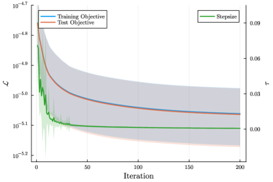
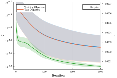
The first experiment aims to compare learning trajectories of the AD-based method 1 and the MM-based method 2 for a fixed combination of network width and depth. The layer configuration is set to be the same as [Shi et al.(2019)Shi, Shi, O’Connell, Yu, Azizzadenesheli, Anandkumar, Yue, and Chung], i.e., . Table 1 shows the root-mean-square (RMS) value of the prediction error for training and test datasets along with the training time in the mean format. Figure LABEL:Fig_E1 shows training/test objectives and the automatically determined stepsize with the mean and interval over 40 different random seeds. Method 1 provides much faster convergence than method 2 while achieving better prediction accuracies with less iterations. The rapid convergence is observed especially in the initial few tens of iterations. It turns out that the stepsize determined by method 2 is about two orders of magnitude smaller than method 1, which is thought to be resulting from the convervative nature of the chosen majorisation. The stepsize trajectory is more smooth and regular in method 2. A remedy is to scale up the stepsize determined by method 2 with a constant factor, however this will introduce a new hyperparameter. The stepsize determined by method 1 does not show significant variations after the initial 50 iterations while showing an overall decreasing pattern without any manual scheduling.
Fig_E1
\subfigure[Method 1 (AD)]
 \subfigure[Method 2 (MM)]
| Method | Training RMS Error [N] | Test RMS Error [N] | Training Time [s] |
|---|---|---|---|
| 1 | / 200 iterations | ||
| 2 | / 3000 iterations |
4.2 Experiment 2. Learning Results for Various Widths/Depths
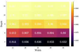
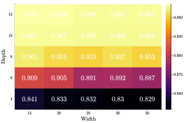
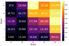
The second experiment aims to show the performance dependency of the AD-based method 1 with iterations on the network widths and depths. We consider a grid over widths and depths to set the layer configuration so that for while and . Figure LABEL:Fig_E2 shows the RMS errors for training and test datasets and the training time with their mean values over 40 different random seeds for each width/depth combination. The heatmaps for the mean RMS errors display consistent trends. First, the proposed method achieves a similar level (N) of prediction accuracies for all layer configurations. Second, for each given depth, increasing width tends to yield smaller RMS errors for both training and test datasets. Third, for each given width, increasing depth tends to yield larger RMS errors. Fourth, the variation of RMS error is larger across different depths than across widths. Lastly, the present benchmark shows that the proposed method is particularly effective for training smaller networks in terms of achieved accuracies with respect to training time.
Fig_E2
\subfigure[Training RMS Error [N]]
 \subfigure[Test RMS Error [N]]
 \subfigure[Training Time [s]]
5 Discussion
This study has proposed automatic optimisation methods for fully-connected neural networks with layerwise normalisation of parameters which specifies the Frobenius norm of the weights for each layer. Since the Frobenius norm can be computed more efficiently than the operator norm and is represented with a simple closed-form expression, evaluation and update of the neural network is easier with Frobenius normalisation than with spectral normalisation. For this type of normalised neural network, the proposed initialisation and update methods provide a complete neural network optimisation workflow that does not require manual tuning of the stepsize while explicitly accounting for the spherical motion of trainable parameters. Experiments on a dynamic model regression problem showed the effectiveness of the Hessian-free second-order stepsize determination method across a broad range of layer width/depth configurations. The proposed method achieved rapid convergence in the initial phase and consistent trends observed in the prediction accuracy without any manual learning rate scheduling or gradient clipping.
References
- [Absil et al.(2008)Absil, Mahony, and Sepulchre] Pierre-Antoine Absil, Robert Mahony, and Rodolphe Sepulchre. Optimization Algorithms on Matrix Manifolds. Princeton University Press, Princeton, NJ, 2008. URL https://sites.uclouvain.be/absil/amsbook/.
- [Anil et al.(2019)Anil, Lucas, and Grosse] Cem Anil, James Lucas, and Roger Grosse. Sorting Out Lipschitz Function Approximation. In 36th International Conference on Machine Learning, pages 291–301, Long Beach, CA, USA, June 2019. URL https://proceedings.mlr.press/v97/anil19a.html.
- [Bartlett et al.(2017)Bartlett, Foster, and Telgarsky] Peter L. Bartlett, Dylan J. Foster, and Matus J. Telgarsky. Spectrally-Normalized Margin Bounds for Neural Networks. In 31st Conference on Neural Information Processing Systems, Long Beach, CA, USA, December 2017. URL https://proceedings.neurips.cc/paper_files/paper/2017/file/b22b257ad0519d4500539da3c8bcf4dd-Paper.pdf.
- [Bernstein et al.(2020)Bernstein, Vahdat, Yue, and Liu] Jeremy Bernstein, Arash Vahdat, Yisong Yue, and Ming-Yu Liu. On the Distance Between Two Neural Networks and the Stability of Learning. In 34th Conference on Neural Information Processing Systems, Virtual, December 2020. URL https://proceedings.neurips.cc/paper/2020/hash/f4b31bee138ff5f7b84ce1575a738f95-Abstract.html.
- [Bernstein et al.(2023)Bernstein, Mingard, Huang, Azizan, and Yue] Jeremy Bernstein, Chris Mingard, Kevin Huang, Navid Azizan, and Yisong Yue. Automatic Gradient Descent: Deep Learning without Hyperparameters, 2023.
- [Bernstein(2023)] Jeremy David Bernstein. Optimisation & Generalisation in Networks of Neurons. PhD thesis, California Institute of Technology, Pasadena, CA, USA, 2023.
- [Boumal(2023)] Nicolas Boumal. An Introduction to Optimization on Smooth Manifolds. Cambridge University Press, Cambridge, UK, 2023. URL https://www.nicolasboumal.net/book/.
- [Cho(2023)] Namhoon Cho. ASGD. GitHub, October 2023. URL https://github.com/nhcho91/ASGD.
- [Landeros et al.(2023)Landeros, Xu, and Lange] Alfonso Landeros, Jason Xu, and Kenneth Lange. MM Optimization: Proximal Distance Algorithms, Path Following, and Trust Regions. Proceedings of the National Academy of Sciences, 120(27):e2303168120, 2023. 10.1073/pnas.2303168120.
- [Lange(2016)] Kenneth Lange. MM Optimization Algorithms. Society for Industrial and Applied Mathematics, Philadelphia, PA, USA, 2016. 10.1137/1.9781611974409.
- [Lin et al.(2021)Lin, Sekar, and Fanti] Zinan Lin, Vyas Sekar, and Giulia Fanti. Why Spectral Normalization Stabilizes GANs: Analysis and Improvements. In 35th Conference on Neural Information Processing Systems, Virtual, December 2021. URL https://proceedings.neurips.cc/paper_files/paper/2021/hash/4ffb0d2ba92f664c2281970110a2e071-Abstract.html.
- [Liu et al.(2020)Liu, Shi, Chung, Anandkumar, and Yue] Anqi Liu, Guanya Shi, Soon-Jo Chung, Anima Anandkumar, and Yisong Yue. Robust Regression for Safe Exploration in Control. In 2nd Conference on Learning for Dynamics and Control, pages 608–619, June 2020. URL https://proceedings.mlr.press/v120/liu20a.html.
- [Liu et al.(2021)Liu, Bernstein, Meister, and Yue] Yang Liu, Jeremy Bernstein, Markus Meister, and Yisong Yue. Learning by Turning: Neural Architecture Aware Optimisation. In 38th International Conference on Machine Learning, pages 6748–6758, Virtual, July 2021. URL https://proceedings.mlr.press/v139/liu21c.html.
- [Martens(2010)] James Martens. Deep Learning via Hessian-Free Optimization. In 27th International Conference on Machine Learning, Haifa, Israel, June 2010. URL https://www.cs.toronto.edu/ jmartens/docs/Deep_HessianFree.pdf.
- [Miyato et al.(2018)Miyato, Kataoka, Koyama, and Yoshida] Takeru Miyato, Toshiki Kataoka, Masanori Koyama, and Yuichi Yoshida. Spectral Normalization for Generative Adversarial Networks. In 6th International Conference on Learning Representations, Vancouver, BC, Canada, April-May 2018. URL https://openreview.net/forum?id=B1QRgziT-.
- [O’Connell et al.(2022)O’Connell, Shi, Shi, Azizzadenesheli, Anandkumar, Yue, and Chung] Michael O’Connell, Guanya Shi, Xichen Shi, Kamyar Azizzadenesheli, Anima Anandkumar, Yisong Yue, and Soon-Jo Chung. Neural-Fly Enables Rapid Learning for Agile Flight in Strong Winds. Science Robotics, 7(66):eabm6597, 2022. 10.1126/scirobotics.abm6597.
- [Pearlmutter(1994)] Barak A. Pearlmutter. Fast Exact Multiplication by the Hessian. Neural Computation, 6(1):147–160, 1994. 10.1162/neco.1994.6.1.147.
- [Roburin et al.(2022)Roburin, de Mont-Marin, Bursuc, Marlet, Pérez, and Aubry] Simon Roburin, Yann de Mont-Marin, Andrei Bursuc, Renaud Marlet, Patrick Pérez, and Mathieu Aubry. Spherical Perspective on Learning with Normalization Layers. Neurocomputing, 487:66–74, 2022. 10.1016/j.neucom.2022.02.021.
- [Shi(2023)] Guanya Shi. Reliable Learning and Control in Dynamic Environments: Towards Unified Theory and Learned Robotic Agility. PhD thesis, California Institute of Technology, Pasadena, CA, USA, 2023.
- [Shi et al.(2019)Shi, Shi, O’Connell, Yu, Azizzadenesheli, Anandkumar, Yue, and Chung] Guanya Shi, Xichen Shi, Michael O’Connell, Rose Yu, Kamyar Azizzadenesheli, Animashree Anandkumar, Yisong Yue, and Soon-Jo Chung. Neural Lander: Stable Drone Landing Control Using Learned Dynamics. In International Conference on Robotics and Automation, pages 9784–9790, Montreal, QC, Canada, May 2019. 10.1109/ICRA.2019.8794351.
- [Shi et al.(2022)Shi, Hönig, Shi, Yue, and Chung] Guanya Shi, Wolfgang Hönig, Xichen Shi, Yisong Yue, and Soon-Jo Chung. Neural-Swarm2: Planning and Control of Heterogeneous Multirotor Swarms Using Learned Interactions. IEEE Transactions on Robotics, 38(2):1063–1079, 2022. 10.1109/TRO.2021.3098436.
- [Streeter(2023)] Matthew Streeter. Universal Majorization-Minimization Algorithms, 2023.
- [Streeter and Dillon(2023)] Matthew Streeter and Joshua V. Dillon. Automatically Bounding the Taylor Remainder Series: Tighter Bounds and New Applications, 2023.
- [Tan(2022)] Songchen Tan. TaylorDiff.jl: Fast Higher-order Automatic Differentiation in Julia, 2022. URL https://github.com/JuliaDiff/TaylorDiff.jl.
- [Tan(2023)] Songchen Tan. Higher-Order Automatic Differentiation and Its Applications. Master’s thesis, Center for Computational Science and Engineering, Massachusetts Institute of Technology, 2023. URL https://hdl.handle.net/1721.1/151501.
- [Wan et al.(2021)Wan, Zhu, Zhang, and Sun] Ruosi Wan, Zhanxing Zhu, Xiangyu Zhang, and Jian Sun. Spherical Motion Dynamics: Learning Dynamics of Normalized Neural Network using SGD and Weight Decay. In 35th Conference on Neural Information Processing Systems, Virtual, December 2021. URL https://proceedings.neurips.cc/paper/2021/hash/326a8c055c0d04f5b06544665d8bb3ea-Abstract.html.
- [Wang and Manchester(2023)] Ruigang Wang and Ian Manchester. Direct Parameterization of Lipschitz-Bounded Deep Networks. In 40th International Conference on Machine Learning, pages 36093–36110, Honolulu, HI, USA, July 2023. URL https://proceedings.mlr.press/v202/wang23v.html.
- [Zhou et al.(2022)Zhou, Pereida, Zhao, and Schoellig] Siqi Zhou, Karime Pereida, Wenda Zhao, and Angela P. Schoellig. Bridging the Model-Reality Gap With Lipschitz Network Adaptation. IEEE Robotics and Automation Letters, 7(1):642–649, 2022. 10.1109/LRA.2021.3131698.