CACTO-SL: Using Sobolev Learning to improve
Continuous Actor-Critic with Trajectory Optimization

Abstract

Trajectory Optimization (TO) and Reinforcement Learning (RL) are powerful and complementary tools to solve optimal control problems. On the one hand, TO can efficiently compute locally-optimal solutions, but it tends to get stuck in local minima if the problem is not convex. On the other hand, RL is typically less sensitive to non-convexity, but it requires a much higher computational effort. Recently, we have proposed CACTO (Continuous Actor-Critic with Trajectory Optimization), an algorithm that uses TO to guide the exploration of an actor-critic RL algorithm. In turns, the policy encoded by the actor is used to warm-start TO, closing the loop between TO and RL. In this work, we present an extension of CACTO exploiting the idea of Sobolev learning. To make the training of the critic network faster and more data efficient, we enrich it with the gradient of the Value function, computed via a backward pass of the differential dynamic programming algorithm. Our results show that the new algorithm is more efficient than the original CACTO, reducing the number of TO episodes by a factor ranging from 3 to 10, and consequently the computation time. Moreover, we show that CACTO-SL helps TO to find better minima and to produce more consistent results.

1 Introduction

Robotic control challenges have long been addressed through Trajectory Optimization (TO). The high-level desired task is encoded in the cost function of an Optimal Control Problem (OCP), which is minimised with respect to the OCP decision variables, which represent the state and control trajectories. Constraints are added to ensure that the solution of the OCP takes into account the robot dynamics, the actuator bounds, and the task-related constraints. When tackling complex problems, the OCP may feature a highly non-convex cost and/or highly nonlinear dynamics. Therefore, gradient-based solvers frequently encounter local minima and are unable to find a globally optimal solution. There exist TO methods based on the Hamilton-Jacobi-Bellman equation or Dynamic Programming, for continuous-time and discrete-time problems respectively, that can find the globally optimal solution. However, these methods are hindered by the curse of dimensionality, which limits their applicability.

With the emergence of deep Reinforcement Learning (RL) and its application to the continuous domain, this machine learning tool is applied more and more widely to robot control problems showing impressive results on continuous state and control spaces [Lillicrap et al.(2015)Lillicrap, Hunt, Pritzel, Heess, Erez, Tassa, Silver, and Wierstra, Fujimoto et al.(2018)Fujimoto, Hoof, and Meger, Haarnoja et al.(2018)Haarnoja, Zhou, Hartikainen, Tucker, Ha, Tan, Kumar, Zhu, Gupta, Abbeel, et al., Schulman et al.(2017)Schulman, Wolski, Dhariwal, Radford, and Klimov]. RL algorithms are less prone to converge to local minima due to their exploratory nature. Yet, there are still several challenges related to the application of RL to robot control, such as the necessity for extensive exploration.

As a potential solution to overcome the limitations of RL and TO, we have recently presented the CACTO algorithm (Continuous Actor-Critic with Trajectory Optimization) [Grandesso et al.(2023)Grandesso, Alboni, Papini, Wensing, and Del Prete]. CACTO iteratively leverages the explorative nature of RL to initialize TO to escape local minima, while exploiting TO to guide the RL exploration. Thanks to the interplay of TO and RL, CACTO’s policy provides TO with initial guesses that allow it to obtain better trajectories than with other initialization techniques. While the use of TO demonstrated to efficiently accelerate convergence, the computational burden associated with solving TO episodes has posed some limitations. In particular, as the system complexity increases, this issue becomes more relevant, hindering the scalability of the algorithm. The ability of TO to produce the Value function’s gradient with limited computational cost presents an opportunity to enhance the algorithm’s data efficiency, by increasing the information extracted from each TO problem. By leveraging Sobolev Learning, the gradient information can be incorporated in the critic’s training, enhancing the performance of the algorithm.

Sobolev spaces are metric spaces where the distance between functions is defined in terms of both the difference between the function values and the difference between their derivatives. The universal approximation theorems for neural networks in Sobolev spaces [Hornik(1991)] show that, under some assumptions, not only a neural network can approximate the value of a function, but also its derivatives with respect to its inputs. This work inspired other research such as [Czarnecki et al.(2017)Czarnecki, Osindero, Jaderberg, Swirszcz, and Pascanu], which extensively studied the employment of the neural network derivatives to improve the training process in different kinds of problems, such as policy distillation and regression on datasets. Sobolev Learning found applications also in the robot control field. For example, in [Parag et al.(2022)Parag, Kleff, Saci, Mansard, and Stasse], this technique is used to learn a Value function to be used as an approximate terminal cost in an OCP, thus allowing to shorten the problem horizon, and speeding up the solver. In [Le Lidec et al.(2023)Le Lidec, Jallet, Laptev, Schmid, and Carpentier], stochastic Sobolev Learning is used to include computationally efficient higher-order information in the policy training, resulting in improved sample efficiency and stability. Even though the use of the derivatives comes with a computational overhead, Sobolev Learning increases robustness against noise, improves generalization and data-efficiency [Masuoka(1993), Lee and Oh(1997)]. In this work, we incorporate Sobolev Learning in CACTO to improve its efficacy and scalability. Our main contributions are:

• We present a new version of the CACTO algorithm that computes the gradient of the Value function using the backward pass of the differential dynamic programming algorithm, and uses it to improve the training of the critic network.

• We show that using ReLU activation functions is detrimental when training the critic with Sobolev learning, and we address this issue by switching to smooth periodical activation functions.

• We integrated our open-source implementation of CACTO with the software libraries CasADi [Andersson et al.(2019)Andersson, Gillis, Horn, Rawlings, and Diehl] (for numerical optimization) and Pinocchio [Carpentier et al.(2019)Carpentier, Saurel, Buondonno, Mirabel, Lamiraux, Stasse, and Mansard] (for multi-body dynamics), making it more versatile and easily accessible by the community.

• We exemplify the behavior of our algorithm in the companion video using a simple 1D toy problem.

2 Method

In [Grandesso et al.(2023)Grandesso, Alboni, Papini, Wensing, and Del Prete], we presented CACTO, an algorithm for finding globally-optimal control policies through TO-guided actor-critic RL, which we summarize in Section 2.1. To increase its computational efficiency, we propose to use Sobolev Learning (SL) [Czarnecki et al.(2017)Czarnecki, Osindero, Jaderberg, Swirszcz, and Pascanu] for training the critic network, as detailed in Section 2.2.

2.1 Original CACTO Formulation

This section presents the former formulation of CACTO, an algorithm to solve discrete-time optimal control problems with a finite horizon, with the following structure: —l—[2]¡b¿ X, U L(X,U) = ∑_t=0^T -1 l_t(x_t,u_t) +  l_T(x_T) x_t+1= f(x_t,u_t)    ∀t=0…T-1 —u_t—≤u_max      ∀t=0…T-1 x_0= x_init where the decision variables are the state and control sequences denoted as $X=x_{0\dots T}$ and $U=u_{0\dots T-1}$, with $x_{t}\in\mathbb{R}^{n}$ and $u_{t}\in\mathbb{R}^{m}$. The cost function $L(\cdot)$ is defined as the sum of the running costs $l_{t}\left(x_{t},u_{t}\right)$ and the terminal cost $l_{T}(x_{T})$. The dynamics, control limits and initial conditions are represented by (2.1), (2.1) and (2.1).

The algorithm begins by solving $N$ TO problems (2.1) with random initial states $x_{init}$, random time horizons in $[1,T]$, and using a classic warm-starting technique, such as initializing all states to $x_{init}$ and all control inputs to zero. For each optimal state computed by TO, we compute the partial $L$-step cost-to-go, where $L$ is the number of lookahead steps used for Temporal Difference (TD) learning, and store them in a replay buffer along with the relative transition (i.e. state, control, and state after $L$ steps). Notice that the states stored in the replay buffer are the augmented states $\tilde{x}=[x,t]$ where $t$ is the time. Next, for $M$ times, a batch of $S$ transitions is sampled from the replay buffer and used to update the neural networks of the critic and the actor. In particular, the critic loss is the mean squared error between the critic’s output and the so-called TD target, while the actor loss is the action-value (i.e. Q) function. Finally, a rollout of the actor’s policy is used to warm-start the TO problems in the next episodes, closing the loop. In [Grandesso et al.(2023)Grandesso, Alboni, Papini, Wensing, and Del Prete], we showed the capabilities of CACTO to escape local minima, while being more computationally efficient than state-of-the-art RL algorithms. Moreover, CACTO has been proven to converge to a global optimum in a discrete-space setting, providing valuable insights into its theoretical principles.

2.2 CACTO with Sobolev Learning (CACTO-SL)

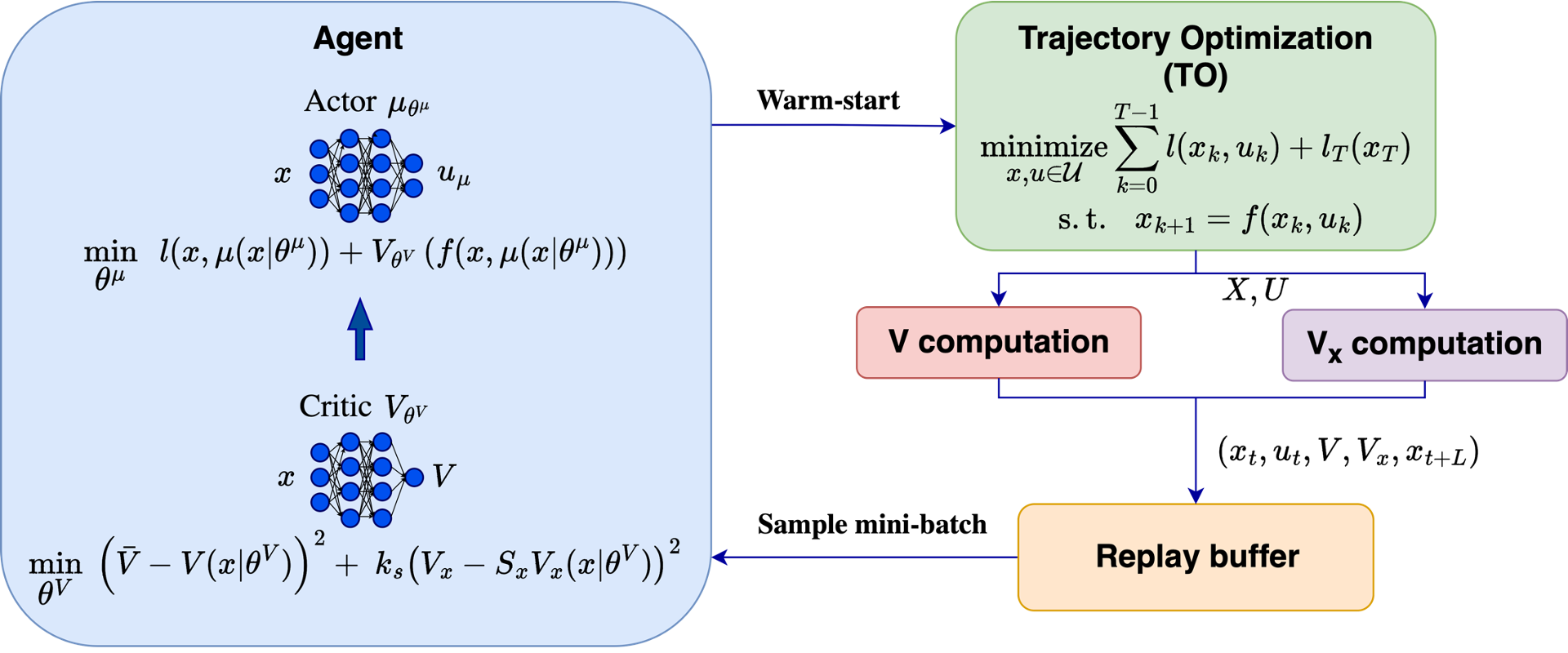
Figure 1: Scheme of the CACTO-SL algorithm.

To exploit Sobolev Learning we need to provide the gradient of the value function with respect to the state: $V_{x}$. To analytically compute $V_{x}$, we use the backward-pass of Differential Dynamic Programming (DDP) [Jacobson(1968), Tassa et al.(2012)Tassa, Erez, and Todorov], an efficient optimal control method for unconstrained nonlinear problems. A scheme of the CACTO-SL algorithm is depicted in Fig. 1. Notice that, since DDP does not handle control bounds, the OCPs solved with CACTO-SL do not feature control bounds, but penalties.

2.2.1 Using the gradient of the Value function in CACTO-SL

To exploit $V_{x}$ when training the critic, we store it in the replay buffer along with the associated transition. Then, during the update-phase, the critic parameters $\theta^{V}$ are updated to approximate both the target values $\bar{V}$ and their gradients $V_{x}$:

$$\operatorname*{minimize}_{\theta^{V}}\quad\frac{1}{S}\sum\limits_{i=1}^{S}\left(\bar{V}_{i}-V(\tilde{x}_{i}|\theta^{V})\right)^{2}+k_{S}\left(V_{x,i}-S_{x}V_{\tilde{x}}(\tilde{x}_{i}|\theta^{V})\right)^{2},$$ (1)

where the matrix $S_{x}=\begin{bmatrix}I_{n\times n}&0_{n}\end{bmatrix}\in\mathbb{R}^{n\times n+1}$ selects the first $n$ elements of the vector $V_{\tilde{x}}(\tilde{x}_{i}|\theta^{V})\in\mathbb{R}^{n+1}$, thus excluding from the error the partial derivative of $V$ w.r.t. time. This is because the state in CACTO is augmented with the time variable, therefore the gradient of the critic w.r.t. its inputs contains also the derivative with respect to time. However, DDP’s backward pass does not compute it because it uses a discrete representation for the time.

The relative importance of the two loss components in (1) is defined by the coefficient $k_{S}$. Tuning $k_{S}$ to achieve the right trade-off between fitting the value and its gradient is important for optimal performance. As $k_{S}$ gets smaller, CACTO-SL tends to behave as the original CACTO algorithm. One may be tempted to set $k_{S}$ to a large value, prioritizing the gradient over the value. This seems sensible because the training of the actor, which is the ultimate goal of the algorithm, relies solely on $V_{x}$. However, we should take into account that the Value function that the critic has to approximate is likely discontinuous. In particular, we can expect discontinuities at the boundaries of the basins of attraction of the different locally-optimal solutions of the OCP. Around discontinuities, the gradient fails to capture the local behavior of the function, therefore setting $k_{S}$ too large may result in extremely poor approximations of the value around discontinuities. This could slow down, or even prevent, convergence to a globally-optimal policy.

To achieve an ideal trade-off between the two loss terms, given the rapid changes and extended range of values taken by $V_{x}$ in the problems we analyzed, we introduce a symmetric logarithmic function in the gradient-related loss:

$$\operatorname*{minimize}_{\theta^{V}}\quad\frac{1}{S}\sum\limits_{i=1}^{S}\left(\bar{V}_{i}-V(\tilde{x}_{i}|\theta^{V})\right)^{2}+k_{S}\left(\text{logsym}(V_{x,i})-\text{logsym}(S_{x}V_{\tilde{x}}(\tilde{x}_{i}|\theta^{V}))\right)^{2},$$ (2)

where the function logsym(x) is defined as

$$\text{logsym}(x)=\begin{cases}\log(x+1)&\text{if }x\geq 0\\ -\log(-x+1)&\text{if }x<0\end{cases}$$ (3)

The logsym(x) function reduces the relative importance of potential large (either positive or negative) values in the gradient, which may arise when the network tries to approximate a discontinuous Value function (see the companion video for a visual illustration of this phenomenon).

Note that our computation of $V_{x}$ corresponds to a Monte-Carlo approach rather than a TD approach, because we do not rely on the gradient of the current critic to compute the target $V_{x}$. Potentially, a customized backward-pass could be designed to compute $V_{x}$ with a TD approach, but we leave this extension to future work.

Alg. 2.2.1 reports the pseudo-code of CACTO-SL, where the differences with respect to the original CACTO formulations have been colored in blue.

[tbp] CACTO-SL Inputs: dynamics $f(\cdot,\cdot)$, running cost $l(\cdot,\cdot)$, terminal cost $l_{T}(\cdot)$, $T$, $M$, $S$, $L$, $\tau$, $e_{update}$, $K_{list}$, $k_{S}$
Output: trained control policy $\mu(\tilde{x})$
$\theta^{V}\leftarrow$ random, $\theta^{\mu}\leftarrow$ random, $\theta^{V^{\prime}}\leftarrow\theta^{V}$
$cycle_{count}\leftarrow 0$
Initialize replay buffer $R$
$episode\leftarrow 1$ $M$ $\tilde{x}_{0}\leftarrow$ random
$\text{episode}<e_{update}$ (   (ICS warm start))$t\leftarrow\tilde{x}_{0}[n]$ $T-1$ $u_{t}\leftarrow 0$
$\tilde{x}_{t+1}\leftarrow\tilde{x}_{0}$  (   (policy rollout))$t\leftarrow\tilde{x}_{0}[n]$ $T-1$ $u_{t}\leftarrow\mu(\tilde{x}_{t}|\theta^{\mu})$
$\tilde{x}_{t+1}\leftarrow[{f}(\tilde{x}_{t}[:n],u_{t}),t+1]$  $x_{0}\leftarrow\tilde{x}_{0}[:n],\quad x\leftarrow\tilde{x}[:\,,\,:n]$
$x,u,l\leftarrow\text{SolveTO}(x_{0},x,u)$
$V_{x}$ = BackwardPass($x,u)\qquad$ (Compute Value’s gradient)
$\tilde{x}[:\,,\,:n]\leftarrow x$
$t\leftarrow\tilde{x}_{0}[n]$ $T$ Compute partial cost-to-go: $V_{t}=\sum\limits_{j=t}^{\min(t+L,T)}\ l_{j}$
Store the transition in the replay buffer: $R\leftarrow(\tilde{x}_{t},V_{t},\mathcolor{blue}{V_{x,t}},\tilde{x}_{\min(t+L,T)})$
$episode$ % $e_{update}=0$ (      (critic $\&$ actor update))$k\leftarrow 1$ $\mathcolor{blue}{K_{list}[cycle_{count}]}$ Sample minibatch of $S$ transitions: $(\tilde{x}_{i},V_{i},\mathcolor{blue}{V_{x,i}},\tilde{x}_{\min(i+L,T)})$
Compute cost-to-go: $\bar{V}_{i}=\begin{cases}V_{i}\quad&\text{if}\,i+L>T\\ V_{i}+V^{\prime}(\tilde{x}_{i+L})\quad&\text{otherwise}\end{cases}$
Update critic by minimizing the loss over $\theta^{V}$:
$L_{c}=\frac{1}{S}\sum\limits_{i=1}^{S}\left(\bar{V}_{i}-V(\tilde{x}_{i}|\theta^{V})\right)^{2}+\mathcolor{blue}{k_{S}\left(\text{logsym}(V_{x,i})-\text{logsym}(S_{x}V_{\tilde{x}}(\tilde{x}_{i}|\theta^{V}))\right)^{2}}$
Update actor by minimizing the loss over $\theta^{\mu}$:
$L_{a}=\frac{1}{S}\sum\limits_{i=1}^{S}l(x_{i},\mu(\tilde{x}_{i}|\theta^{\mu}))+V(f(x_{i},\mu(\tilde{x}_{i}|\theta^{\mu}))|\theta^{V})$
Update target critic: $\theta^{V^{\prime}}\leftarrow\tau\theta^{V}+\left(1-\tau\right)\theta^{V^{\prime}}$
$\mathcolor{blue}{cycle_{count}=cycle_{count}+1}$

2.2.2 Differentiability of the Critic Network

The original CACTO algorithm used ReLU activation functions for both the actor and critic networks. In CACTO-SL, we have observed that ReLU activation functions do not work well in combination with Sobolev Learning. Indeed, the ReLU function leads to piecewise-linear approximations, for which the gradient information may not represent well the local behavior of the function. For this reason, in CACTO-SL the critic network uses SIREN (Sinusoidal Representation Networks) layers [Sitzmann et al.(2020)Sitzmann, Martel, Bergman, Lindell, and Wetzstein]. Characterized by its smooth and continuously differentiable nature, SIREN layers bring a crucial advantage to learning the gradient, preventing the generation of ill-behaved gradients from the loss term on the derivative mismatch.

2.2.3 Sample Efficiency

By incorporating the Value gradient, the amount of information provided by each transition is much higher than in CACTO: each transition contains both the value of the partial cost-to-go (1 scalar) and the gradient of the Value function (an $n$-dimensional vector). Therefore, while ensuring sufficient exploration of the state space is still necessary, we can expect fewer TO episodes to be needed for learning a good approximation of the Value function. This was empirically confirmed by the fact that we could benefit from increasing the ratio between the number of network updates and the number of TO episodes. In particular, we increased the value of $e_{update}$, so as to decrease the frequency of update of the networks, moving towards a pure Policy Iteration scheme [Sutton and Barto(2018)]. Moreover, we modify the value of $K$ during the algorithm. We start with a small value of $K$, because it is not useful to accurately learn the initial policy, which represents the TO solver. As the algorithm progresses, we increase $K$, performing more network updates after each TO-phase, as the accumulated data are expected to represent the Value function of a policy closer and closer to global optimality. This strategic adjustment enables a significant reduction in the number of TO episodes (by a factor of 3 to 10) and, as a consequence, in the computation time.

2.2.4 Software for Trajectory Optimization and Multi-Body Dynamics

While CACTO relied on Pyomo [Nicholson et al.(2018)Nicholson, Siirola, Watson, Zavala, and Biegler] for solving TO problems, CACTO-SL switched to CasADi [Andersson et al.(2019)Andersson, Gillis, Horn, Rawlings, and Diehl], an open-source Automatic Differentiation framework for numerical optimization. By leveraging its symbolic framework and automatic differentiation capabilities, CasADi enables efficient computation of the cost function’s derivatives, required for implementing Sobolev-Learning. Moreover, CasADi is compatible with Pinocchio [Carpentier et al.(2019)Carpentier, Saurel, Buondonno, Mirabel, Lamiraux, Stasse, and Mansard], a versatile rigid-body dynamics library, which freed us from the burden of hand-coding the system dynamics. Each TO problem is transcribed using collocation, and then solved with the nonlinear optimization solver IpOpt [Wächter and Biegler(2006)]. Finally, to speed up the code, we parallelized the generation of the warm-start trajectories, the TO problems, and the computation of the cost to go and its gradient.

3 Results

This section presents our empirical results, with the goal to understand whether the use of Sobolev-Learning in CACTO is actually beneficial. The ability of CACTO-SL to provide good warm-starts to TO problems is analysed in the same scenarios presented in [Grandesso et al.(2023)Grandesso, Alboni, Papini, Wensing, and Del Prete]. The source code is available on the https://github.com/gianluigigrandesso/cactoGitHub page of the project. Before delving into the tests, we suggest the interested readers to check out the https://youtu.be/zAv8dP8itpMcompanion video which exemplifies the behavior of CACTO and the effect of Sobolev Learning using a 1D toy problem.

The analysed task consists in reaching in the shortest time a desired final position, while avoiding three ellipse-shaped obstacles, and minimizing the control effort. The task is described by the following running cost:

$$l(x,u)= \underbrace{w_{d}||p_{ee}-p_{g}||^{2}\vphantom{\frac{w_{p}}{\alpha_{1}}}}_{l_{1}(x)}+\underbrace{-\frac{w_{p}}{\alpha_{1}}\ln(e^{-\alpha_{1}\left(\sqrt{(x_{ee}-x_{g})^{2}+c_{2}}+\sqrt{(y_{ee}-y_{g})^{2}+c_{3}}+c_{4}\right)}+1)}_{l_{2}(x)}+$$ (4)

$$+\underbrace{\frac{w_{ob}}{\alpha_{2}}\sum_{i=1}^{3}\ln{(e^{-\alpha_{2}\left(\frac{(x_{ee}-x_{ob,i})^{2}}{(a_{i}/2)^{2}}+\frac{(y_{ee}-y_{ob,i})^{2}}{(b_{i}/2)^{2}}-1\right)}+1)}}_{l_{3}(x)}+\underbrace{w_{u}||u||_{2}^{2}\vphantom{\sum_{i=1}^{3}}}_{l_{4}(u)}+\underbrace{\left\|\frac{u}{u_{max}}\right\|_{2}^{10}\vphantom{\sum_{i=1}^{3}}}_{l_{5}(u)}$$

where $l_{1}$ penalizes the distance between $p_{ee}=(x_{ee},y_{ee})$ (the x-y coordinate of the system’s end-effector) and $p_{g}$ (the goal position to be reached); $l_{2}$ encodes a cost valley in the neighborhood of the goal position; $l_{3}$ penalizes collision with the three obstacles centered in $p_{ob,i}=(x_{ob,i},y_{ob,i})$ with axes $a_{i}$, and $b_{i}$; the $w_{*}$’s are user-defined weights; $c_{2}$, $c_{3}$, $c_{4}$, $\alpha_{1}$, and $\alpha_{2}$ are the parameters of the softmax functions; $l_{4}$ and $l_{5}$ are the control regularization and penalty to ensure that the optimal controls are in the desired range. The terminal cost is equal to the running cost, except for $l_{4}$ and $l_{5}$. Fig. 2 depicts the cost function, neglecting the control-effort term and control-penalty.

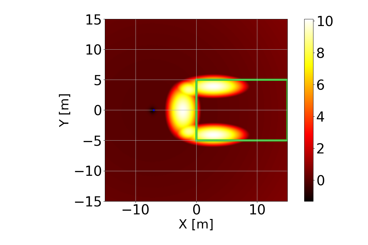
Figure 2: Cost function (4) without the control effort term, considering a target at $p_{g}=[-7,0]$ with weights $w_{d}=10^{-3}$, $w_{p}=5$ and $w_{ob}=10^{1}$. The green rectangle delimits the Hard Region.

The task is designed to ensure the presence of many local minima. In particular, if the system starts from the Hard Region, highlighted by a green rectangle in Fig. 2, it is very hard for the solver to provide a globally-optimal solution. In all our tests, we compute the critic targets with TD(50) (i.e. $L=50$), which empirically led to a stable training of critic and actor.

Figure 3: Comparison of critic networks based on ReLU (top), ELU (middle) and sinusoidal (bottom) activation functions at 1000, 5000 and 10000 updates for a point mass with single integrator dynamics.

3.1 Comparison between activation functions

We compared the critic network based on SIREN layers with the critic networks based on ReLU and based on ELU, another smooth activation layer, in combination with Sobolev Learning using $k_{S}=10^{3}$. Fig. 3 shows that using the SIREN layers (or also ELU layers, but to a slightly lower extent) leads to a critic that clearly captures the lower values of states inside the C-shaped obstacle. On the other hand, this is completely overlooked by the critic using ReLU functions, even after 10000 iterations.

3.2 Comparison between CACTO-SL and CACTO

The comparison between CACTO-SL and CACTO is conducted with a 2D double integrator, and a Dubins car, using $k_{s}=10^{3}$. We compared the algorithms by computing the mean cost of the trajectories obtained by initializing TO with the policy’s rollout. We used as initial states a grid of points over the analysed XY space, with mesh size equal to 1 m. The analysis focuses on the Hard Region ($x\in[0,15]$ m and $y\in[-5,5]$ m). For an easier interpretation of the results, the initial velocity of the system is set to zero. In the Dubins car test, the initial heading is randomly chosen. For each test, we performed 5 runs using the same seeds for both CACTO and CACTO-SL to minimize the effect of the network initialization.

3.2.1 Double-integrator system

We consider a 2D double integrator, with state vector $[x,y,v_{x},v_{y},t]\in\mathbb{R}^{5}$ and control vector $[a_{x},a_{y}]\in\mathbb{R}^{2}$. The maximum episode length is 10 s. The target point is $p_{g}=[-7,0]$. In contrast to the previous version of CACTO, where we alternated $e_{update}=25$ TO episodes and $K=80$ network updates, in CACTO-SL we perform $e_{update}=200$ TO episodes and an increasing number of network updates, starting from $K=1000$ up to $K=15000$. Fig. 4 reports the median (across 5 runs) of the mean cost (across initial conditions) starting from the Hard Region against the number of TO episodes obtained initializing the TO problems with CACTO and CACTO-SL. In both cases, we stopped the training after 50k updates, when both algorithms have converged to a stable TO solution.

Figure 4: Median (across 5 runs) of the mean cost (across initial conditions) starting from the Hard Region with zero initial velocity against the number of TO episodes for a point mass with double integrator dynamics (top) and a Dubins car (bottom). The shaded area represents the area between the first and third quartiles.

Fig. 4 shows that CACTO-SL has led to a 92$\%$ reduction in the number of TO problems. As regards the computation time, it is important to recall that it heavily depends on the algorithm implementation, on the hardware, and on the number of cores used in the parallelization. Parallelizing the execution on 10 cores, the decrease of TO problems has resulted in a reduction of just 7$\%$ of the total execution time because the system is quite simple. However, without parallelization, the total computation time is reduced from 111 to 49 minutes. Moreover, Fig. 4 shows a significant reduction in the variance across the five runs. This outcome can be attributed to the enhanced training of the critic through Sobolev Learning. The improved training results in a more consistent set of critic networks. As a consequence, the actors converge towards similar policies, leading to a more uniform initial guess across runs.

3.2.2 Car system

The second problem involves a Dubins car modelled as a point mass. The 6D state vector consists in the displacement along x and y, angular displacement, linear velocity, linear acceleration and time. The 2D control vector contains the angular velocity and the linear jerk. The car should reach the target point $p_{g}=[-7,0]$ m. No penalty is added on its orientation. We updated the networks every $e_{episode}=500$ TO episodes, using an increasing number of updates, starting from $K=1000$ and reaching up to $K=15000$. In CACTO instead the ratio between TO episodes and network updates was 25/160. Fig. 4 shows the results. In this case, 170k updates have been performed.

In this case, CACTO-SL leads to a notable reduction in the number of TO problems solved and, consequently, in computation times, from 10 h to 6.30 h (parallelizing the TO problems on 10 cores). Note that the reduction in computation time increases significantly also with parallelization, even though the Dubins car has only one more state than the 2D double integrator. Also in this test, Sobolev Learning plays an important role in achieving smaller variance across the runs.

4 Conclusions

This paper presented CACTO-SL, an extension of the CACTO algorithm, featuring Sobolev Learning. CACTO-SL efficiently computes the gradient of the Value function using the backward pass of the DDP algorithm, and exploits this information to improve the training of the critic network. Our results show that this makes CACTO-SL significantly more sample efficient than CACTO, reducing the number of TO episodes by a factor ranging from 3 to 10. This also leads to almost halving the computation time required to reach a stable solution. Moreover, our results show that CACTO-SL reduces the variance of the algorithm across different runs, and helps TO to find better minima.

In the future, we plan to switch to a BoxDDP backward pass [Tassa et al.(2014)Tassa, Mansard, and Todorov], which would allow us to consider hard bounds on the control inputs. Moreover, we are exploring different approaches to bias the sampling of initial states towards more informative state regions, which should improve even further the sample efficiency of CACTO and allow us to scale better to more complex systems.

This work was supported by PRIN project DOCEAT (CUP n. E63C22000410001).

References

- [Andersson et al.(2019)Andersson, Gillis, Horn, Rawlings, and Diehl] Joel A E Andersson, Joris Gillis, Greg Horn, James B Rawlings, and Moritz Diehl. CasADi – A software framework for nonlinear optimization and optimal control. Mathematical Programming Computation, 11(1):1–36, 2019. 10.1007/s12532-018-0139-4.
- [Carpentier et al.(2019)Carpentier, Saurel, Buondonno, Mirabel, Lamiraux, Stasse, and Mansard] Justin Carpentier, Guilhem Saurel, Gabriele Buondonno, Joseph Mirabel, Florent Lamiraux, Olivier Stasse, and Nicolas Mansard. The pinocchio c++ library – a fast and flexible implementation of rigid body dynamics algorithms and their analytical derivatives. In IEEE International Symposium on System Integrations (SII), 2019.
- [Czarnecki et al.(2017)Czarnecki, Osindero, Jaderberg, Swirszcz, and Pascanu] Wojciech M Czarnecki, Simon Osindero, Max Jaderberg, Grzegorz Swirszcz, and Razvan Pascanu. Sobolev training for neural networks. Advances in neural information processing systems, 30, 2017.
- [Fujimoto et al.(2018)Fujimoto, Hoof, and Meger] Scott Fujimoto, Herke Hoof, and David Meger. Addressing function approximation error in actor-critic methods. In International conference on machine learning, pages 1587–1596. PMLR, 2018.
- [Grandesso et al.(2023)Grandesso, Alboni, Papini, Wensing, and Del Prete] Gianluigi Grandesso, Elisa Alboni, Gastone P. Rosati Papini, Patrick M. Wensing, and Andrea Del Prete. Cacto: Continuous actor-critic with trajectory optimization—towards global optimality. IEEE Robotics and Automation Letters, 8(6):3318–3325, 2023. 10.1109/LRA.2023.3266985.
- [Haarnoja et al.(2018)Haarnoja, Zhou, Hartikainen, Tucker, Ha, Tan, Kumar, Zhu, Gupta, Abbeel, et al.] Tuomas Haarnoja, Aurick Zhou, Kristian Hartikainen, George Tucker, Sehoon Ha, Jie Tan, Vikash Kumar, Henry Zhu, Abhishek Gupta, Pieter Abbeel, et al. Soft actor-critic algorithms and applications. arXiv preprint arXiv:1812.05905, 2018.
- [Hornik(1991)] Kurt Hornik. Approximation capabilities of multilayer feedforward networks. Neural networks, 4(2):251–257, 1991.
- [Jacobson(1968)] David H Jacobson. New second-order and first-order algorithms for determining optimal control: A differential dynamic programming approach. Journal of Optimization Theory and Applications, 2:411–440, 1968.
- [Le Lidec et al.(2023)Le Lidec, Jallet, Laptev, Schmid, and Carpentier] Quentin Le Lidec, Wilson Jallet, Ivan Laptev, Cordelia Schmid, and Justin Carpentier. Enforcing the consensus between trajectory optimization and policy learning for precise robot control. In 2023 IEEE International Conference on Robotics and Automation (ICRA), pages 946–952. IEEE, 2023.
- [Lee and Oh(1997)] Jeong-Woo Lee and Jun-Ho Oh. Hybrid learning of mapping and its jacobian in multilayer neural networks. Neural computation, 9(5):937–958, 1997.
- [Lillicrap et al.(2015)Lillicrap, Hunt, Pritzel, Heess, Erez, Tassa, Silver, and Wierstra] Timothy P Lillicrap, Jonathan J Hunt, Alexander Pritzel, Nicolas Heess, Tom Erez, Yuval Tassa, David Silver, and Daan Wierstra. Continuous control with deep reinforcement learning. arXiv preprint arXiv:1509.02971, 2015.
- [Masuoka(1993)] Ryusuke Masuoka. Noise robustness of ebnn learning. In Proceedings of 1993 International Conference on Neural Networks (IJCNN-93-Nagoya, Japan), volume 2, pages 1665–1668. IEEE, 1993.
- [Nicholson et al.(2018)Nicholson, Siirola, Watson, Zavala, and Biegler] Bethany Nicholson, John D. Siirola, Jean Paul Watson, Victor M. Zavala, and Lorenz T. Biegler. Pyomo.Dae: a Modeling and Automatic Discretization Framework for Optimization With Differential and Algebraic Equations. Mathematical Programming Computation, 10(2):187–223, 2018. ISSN 18672957. 10.1007/s12532-017-0127-0. URL https://doi.org/10.1007/s12532-017-0127-0.
- [Parag et al.(2022)Parag, Kleff, Saci, Mansard, and Stasse] Amit Parag, Sébastien Kleff, Léo Saci, Nicolas Mansard, and Olivier Stasse. Value learning from trajectory optimization and sobolev descent: A step toward reinforcement learning with superlinear convergence properties. In 2022 International Conference on Robotics and Automation (ICRA), pages 01–07, 2022. 10.1109/ICRA46639.2022.9811993.
- [Schulman et al.(2017)Schulman, Wolski, Dhariwal, Radford, and Klimov] John Schulman, Filip Wolski, Prafulla Dhariwal, Alec Radford, and Oleg Klimov. Proximal policy optimization algorithms. arXiv preprint arXiv:1707.06347, 2017.
- [Sitzmann et al.(2020)Sitzmann, Martel, Bergman, Lindell, and Wetzstein] Vincent Sitzmann, Julien Martel, Alexander Bergman, David Lindell, and Gordon Wetzstein. Implicit neural representations with periodic activation functions. In H. Larochelle, M. Ranzato, R. Hadsell, M.F. Balcan, and H. Lin, editors, Advances in Neural Information Processing Systems, volume 33, pages 7462–7473. Curran Associates, Inc., 2020. URL https://proceedings.neurips.cc/paper_files/paper/2020/file/53c04118df112c13a8c34b38343b9c10-Paper.pdf.
- [Sutton and Barto(2018)] Richard S. Sutton and Andrew G. Barto. Reinforcement Learning: An Introduction. The MIT Press, second edition, 2018. URL http://incompleteideas.net/book/the-book-2nd.html.
- [Tassa et al.(2012)Tassa, Erez, and Todorov] Yuval Tassa, Tom Erez, and Emanuel Todorov. Synthesis and stabilization of complex behaviors through online trajectory optimization. In Intelligent Robots and Systems (IROS), IEEE/RSJ International Conference on, pages 4906–4913, 2012. ISBN 9781467317351. URL https://dada.cs.washington.edu/homes/todorov/papers/MPCGetUp.pdf.
- [Tassa et al.(2014)Tassa, Mansard, and Todorov] Yuval Tassa, Nicolas Mansard, and Emo Todorov. Control-limited differential dynamic programming. In Proceedings - IEEE International Conference on Robotics and Automation, pages 1168–1175, 2014. ISBN 9781479936854. 10.1109/ICRA.2014.6907001.
- [Wächter and Biegler(2006)] Andreas Wächter and Lorenz T Biegler. On the implementation of an interior-point filter line-search algorithm for large-scale nonlinear programming. Mathematical programming, 106:25–57, 2006.