Heuristics and Metaheuristics for Dynamic Management of Computing and Cooling Energy in Cloud Data Centers

Abstract

[Abstract] Data centers handle impressive high figures in terms of energy consumption, and the growing popularity of Cloud applications is intensifying their computational demand. Moreover, the cooling needed to keep the servers within reliable thermal operating conditions also has an impact on the thermal distribution of the data room, thus affecting to servers’ power leakage. Optimizing the energy consumption of these infrastructures is a major challenge to place data centers on a more scalable scenario. Thus, understanding the relationship between power, temperature, consolidation and performance is crucial to enable an energy-efficient management at the data center level. In this research, we propose novel power and thermal-aware strategies and models to provide joint cooling and computing optimizations from a local perspective based on the global energy consumption of metaheuristic-based optimizations. Our results show that the combined awareness from both metaheuristic and best fit decreasing algorithms allow us to describe the global energy into faster and lighter optimization strategies that may be used during runtime. This approach allows us to improve the energy efficiency of the data center, considering both computing and cooling infrastructures, in up to a 21.74% while maintaining quality of service.

1 Introduction

Nowadays, data centers consume about the 2% of the worldwide energy production ¹², originating more than 43 million tons of $CO_{2}$ per year ¹⁹. Also, the proliferation of urban data centers is responsible for the increasing power demand of up to 70% in metropolitan areas, where the power density is becoming too high for the power grid ¹¹. In two years, the 95% of the urban data centers will experience partial or total outages, incurring in annual costs of about US$2 million per infrastructure. The 28% of these service outages are expected to appear due to exceeding the maximum capacity of the grid ³². The advantages of Cloud computing lie in the usage of a technological infrastructure that allows high degrees of automation, consolidation and virtualization, which results in a more efficient management of the resources of a data center. Cloud computing, in the context of data centers, has been proposed as a mechanism for minimizing environmental impact. Virtualization and consolidation increase hardware utilization (of up to $80\%$ ¹⁶) thus improving resource efficiency. Moreover, a cloud usually consists of distributed resources dynamically provisioned as services to the users, so it is flexible enough to find matches between different parameters to reach performance optimizations. Gartner expectations predict that by 2020, Cloud adoption strategies would impact on more than the 50% of the IT (Information Technology) outsourcing deals in an effort to cost optimize the infrastructures that use from 10 to 100 times more power than typical office buildings ³⁷ even consuming as much electricity as a city ²⁴.

The main contributors to the energy consumption in a data center are: (i) the IT resources, which consist of servers and other IT equipment, and (ii) the cooling infrastructure needed to ensure that the IT operates within a safe range of temperatures, ensuring reliability. The remaining 10% comes from (iii) the power consumption that comes from lightning, generators, uninterruptible power supply systems and power distribution units ¹⁹. The IT power in the data center is dominated by the power consumption of the enterprise servers, representing up to 60% of the overall data center consumption. The power usage of an enterprise server can be divided into dynamic and static contributions. On the other hand, the cooling infrastructure is one of the major contributors to the overall data center power budget, representing around $40\%$ of the total power consumed by the entire facility ¹³. This is the main reason why recent research aim to achieve new thermal-aware techniques to optimize the temperature distribution in the facility, thus minimizing the cooling costs. Controlling the set point temperature of cooling systems in data centers is still to be clearly defined and it represents a key challenge from the energy perspective. This value is often chosen based on conservative suggestions provided by the manufacturers of the equipment and it is calculated for the worst case scenario resulting in overcooled facilities. Increasing the temperature results in savings in cooling consumption, so a careful management can be devised ensuring a safe temperature range for IT resources. From the application-framework viewpoint, Cloud workloads present additional restrictions as 24/7 availability, and SLA (Service Level Agreement) constraints among others. In this computing paradigm, workloads hardly use the 100% of the CPU (Central processing unit) resources, and their runtime is strongly constrained by contracts between Cloud providers and clients. These restrictions have to be taken into account when minimizing the energy consumption as they impose additional boundaries to the optimization strategies.

Just for an average $100kW$ data center, a $7\%$ in annual savings represents around US $5 million per year ⁹. These power and thermal situations have encouraged the challenges in the data center scope to be extended from performance, which used to be the main target, to energy-efficiency. This context draws the priority of stimulating researchers to develop sustainability policies at the data center level, in order to achieve a social sense of responsibility, while minimizing environmental impact. However, current approaches do not incorporate the impact of leakage consumption, found at the technology level, when controlling the cooling set point temperature at the data center level. This power contribution, which grows for increasing temperatures, is neither considered when optimizing allocation strategies in terms of energy under highly variable workloads, typically found in Cloud environments. Thus, using power and thermal models that incorporate this information at different abstraction levels, which impacts on the power contributors, helps us to find the relationships required to devise a global minimization searching for the optimum that combines power and thermal-aware strategies for joint IT and cooling infrastructures. For this purpose, we evaluate the use of metaheuristic-based algorithms that provide a global minimization. In our work, we will focus on the combination of strategies that are aware of both IT and cooling consumption, also taking into account the thermal impact and the resource variability.

This work is intended to offer novel optimization strategies that take into account the contributions to power of non-traditional parameters such as temperature and frequency among others. Our research is based on fast and accurate models that are aware of the relationships with power of these parameters, allowing us to combine both energy and thermal-aware strategies. Our work makes the following key contributions: 1) a set of single-objective and multi-objective BFD (Best Fit Decreasing)-based policies that optimize the energy consumption of the data center considering both IT and cooling parameters; 2) a metaheuristic-based optimization policy that relies in a simulated annealing algorithm to optimize the energy consumption of both IT and cooling infrastructures; 3) a novel strategy to infer a local minimization based on modeling the improvements provided by the simulated annealing optimization; 4) two thermal models that accurately describe the behavior of the CPU and the memory devices, resulting in an average temperature estimation error of 0.85% and 0.50% respectively; and 5) a cooling strategy based on the estimated temperature of devices due to VM (Virtual Machine) allocation. The remainder of this paper is organized as follows: Section 2 gives further information on the related work on this topic. Our proposed optimization framework and VM consolidation algorithms are provided in Sections 3 and 4 . Section 5 and Section 6 explain the modeling process for our metaheuristic-based VM consolidation policy and our cooling strategy respectively. Section 7 describes profusely the experimental results. Finally, in Section 8 the main conclusions are drawn.

2 Related Work

Due to the impact of energy-efficient optimizations in an environment that handles so impressive high figures as data centers, many researchers have been motivated to focus their academic work on obtaining solutions for reducing consumption. In this section, we present different approaches of the state-of-the-art based on heuristics and metaheuristics that are aware of energy contributions.

2.1 Reduce IT power consumption

Power minimization, resource utilization and Quality of Service (QoS) are the main targets in energy-efficient strategies for Cloud data centers ⁴¹, ⁴², ³¹. Different heuristic algorithms have been used to solve the VM placement as a bin packing problem. First fit decreasing and Best Fit Decreasing (BFD) policies have been used to minimize the IT energy consumption from a local perspective ¹⁰, ⁶, ²⁰, ³⁹. These approaches mainly consider the optimization of a single-objective scenario under certain QoS constraints. On the other hand, metaheuristics are also applied to manage the allocation of each VM in vmList will be allocated in the server provided by the best solution. VMs in Cloud computing ². Wu et al. ⁴³ proposes the use of a single-objective GA (Genetic Algorithm) to optimize IT energy consumption. These metaheuristic-based approaches can be used to solve the problem from a global perspective (considering the consumption of the whole IT infrastructure), also targeting more than one optimization objectives. Ye et al. ⁴⁵ propose a KnEA-based evolutionary algorithm considering, not only energy consumption and resource utilization, but also load balance and robustness objectives simultaneously.

2.2 Joint Thermal and Power-Aware considerations

Currently, data centers save lots of energy by providing efficient cooling mechanisms. Hot-spots throughout the facilities are the main drawback according to system failures, and due to this factor, some data centers maintain very low room temperatures of up to 13${}^{\circ}C$ ¹⁶. Most recently, data centers are turning towards new efficient cooling systems that make higher temperatures possible, around 24${}^{\circ}C$ or even 27${}^{\circ}C$. The increasing power density of new technologies has resulted in the incapacity of processors to operate at maximum design frequency, while transistors have become extremely susceptible to errors causing system failures ²⁶. Moreover, adding to this issue that system errors increase exponentially with temperature, new techniques that minimize both effects are required. To avoid these thermal-related issues while further reducing energy, researchers are mainly focusing on considering the power consumption of servers’ fans, the power leakages due to temperature and the power due to air conditioning units.

2.2.1 Servers fan power consumption

Ayoub et al. ⁵ and Chan et al. ⁸ propose energy-aware heuristics considering joint fan control and scheduling mechanisms to reduce consumption of a server. Their work propose a state machine to simultaneously minimize several objectives. They provide models to estimate temperature that use electrical analogies to represent the thermal behavior of the components.

2.2.2 Power Leakage due to temperature

In current electronic systems, in which integration technology scales below 100nm, static power consumption represents about 30-50% ²⁹, of the total power under nominal conditions. The impact of temperature, which presents an exponential dependency on the leakage currents ³⁶, aggravates this situation increasing power consumption. Some Cloud computing solutions have taken into account the dependence of power consumption with temperature, due to both fan speed and induced leakage currents. In our previous work ⁴, we present a power model that includes both contributions, which we used to provide energy savings together with a DVFS-aware allocation strategy ³. In the present research, we aim to improve energy efficiency by extending this VM allocation policy, also incorporating thermal-awareness. Li et al. ²² also provide an heuristic that minimizes power consumption, using a model that depends on fan power and leakage.

2.2.3 Power of Air Conditioning Units

The power budget to cool down data center infrastructures represents about the 40% of the total budget ¹³. By combining energy-aware strategies in both computing and cooling infrastructures, potential savings of about $54\%$ ³⁰ are estimated. Thus, researchers are including the effects of temperature in the data room among their optimization objectives. On its own, virtualization has the potential of minimizing the hot-spot issue by migrating VMs. Migration policies allow to distribute the workload during run-time without stopping task execution. Primas et al. ³³ present an heuristic to perform energy-efficient scheduling considering the temperature of the data room. Xu et al. ⁴⁴ present a GA-based multi-objective VM placement algorithm that targets power consumption, resource wastage and thermal dissipation costs. In both research works, the energy consumption of the cooling infrastructure is not calculated but they assume a significant reduction due to reducing hot spots using load balancing.

On the other hand, there are research works in which the power of air conditioning units is minimized explicitly together with the IT power. Abbasi et al. ¹ propose heuristic algorithms to address this problem. Their work presents the data center as a distributed cyber physical system in which the energy of both IT and cooling is the minimization objective. Li et al. ²³ use a greedy scheduling algorithm, considering the temperature distribution airflow to minimize the energy consumption of IT and cooling jointly. Current research in the area of joint energy and thermal aware strategies consider fan power, leakage due to temperature or cooling units’ power, but do not take into account the combined effects between them. Our work proposes the global minimization of the energy of the entire facility (IT and cooling infrastructures) considering all these thermal effects and their impact on power consumption in a proactive way.

3 Optimization paradigm

The new simulation and optimization framework presented in this research considers the energy of a Cloud data center from a global and proactive perspective. So, our proposed optimization algorithms are aware of the evolution of the global energy demand, the thermal behavior of the room and the workload considerations at the different data center subsystems during runtime. This section explains our hypothesis on how to provide a feasible and proactive solution to approach the issues that have been motivated. The scenario chosen for the development of this research, is a Cloud optimization framework that can be seen in Figure 1. The applications require constant monitoring of their computational demand in order to capture their variability during runtime and to perform VM migrations when needed in order to avoid QoS degradation.

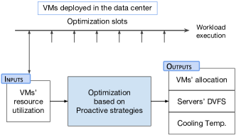
Figure 1: Overview of the inputs and outputs of the proposed optimization framework.

As during this research work we did not have access to an operative Cloud data center, we leverage real traces publicly released by Cloud providers to simulate the operation of the infrastructure. These traces consist of periodic resource usage reports that provide specific information as CPU demand percentages and memory and disk usage and provisioning values for all VMs. These traces are the only input for our optimization framework, based on proactive strategies. Finally, for each optimization slot, we obtain the allocation for the VMs in the system, as well as the servers’ DVFS configuration and the cooling set point temperature. In Figure 2, we present our proposed optimization based on proactive strategies more in detail. For each optimization slot, in which we have input traces, we detect overloaded hosts for the current placement of VMs that are already deployed on the system, where oversubscription is allowed. Overloaded hosts are more likely to suffer from performance degradation, so some VMs have to be migrated from them to other hosts.

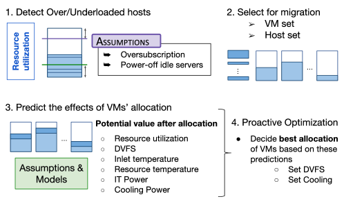
Figure 2: Overview of the optimization diagram for the proposed framework.

Based on this information, the consolidation algorithm selects: 1) the set of VMs that have to be migrated from the overloaded physical machines and 2) the set of servers that are candidates to host these VMs. Then, the models help to predict the effects of potential allocations for the set of VMs. These models are needed to provide values of both the parameters that are observed in the infrastructure (temperature and power of the different resources) and the control variables (VM placement, DVFS and cooling set point temperature). Finally, the proactive optimization algorithm decides the best allocation of VMs based on these predictions. After this first iteration, if underloaded hosts are found, this optimization process is repeated in order to power off idle servers if possible. We assume this data center may be homogeneous in terms of IT equipment. Live migration, oversubscription of CPU, DVFS and automatic scaling of the active servers’ set are enabled. We assume a traditional hot-cold aisle data center layout with CRAC (Computer Room Air Conditioning)-based cooling. In particular, at the data center level we consider a raised-floor air-cooled infrastructure where cold air is supplied via the floor plenum and extracted in the ceiling.

4 Description of VM Allocation Strategies

The different policies presented in this section are based on the knowledge achieved from our power model presented in our previous research ⁴ for a Fujitsu RX300 S6 server, that is further explained in Section 7 and can be seen in Equation 8. In this section we provide a taxonomy of candidate optimization algorithms that take into account IT and cooling power of the data center infrastructure under energy and thermal considerations. The mathematical description of these objectives will allow the later optimization by the development of an optimization algorithm.

4.1 Single-Objective BFD-based Allocation Policies

These Single-Objective (SO) policies optimize the consolidation of a set of VMs ($vmList$) using the BFD approach. First, VMs are sorted in decreasing order of CPU utilization and then, they are allocated on the set of available hosts ($hostList$) according to the minimization of an optimization objective that is calculated by the function $SOvalue()$ as can be seen in Algorithm 1. This function computes the single objective according to the model selected from those presented in the following Subsections 4.1.1- 4.1.8. $bestPlacement$ and $bestHost$ are the best placement value for each iteration and the best host to allocate the VM respectively.

Algorithm 1 SO Placement Policy

1:hostList, vmList

2:SOPlacement of VMs

3:vmList.sortDecreasingUtilization()

4:foreach vm in vmList do

5:     bestPlacement $\leftarrow$ MAX

6:     bestHost $\leftarrow$ NULL

7:     foreach host in hostList do

8:         if host has enough resources for vm then

9:              placement $\leftarrow$ SOvalue()

10:              if placement $<$ bestPlacement then

11:                  bestHost $\leftarrow$ host

12:                  bestPlacement $\leftarrow$ placement

13:              end if

14:         end if

15:     end for

16:     if bestHost $\neq$ NULL then

17:         SOPlacement.add(vm, bestHost)

18:     end if

19:end for

20:Return: SOPlacement

Then, each VM in $vmList$ will be allocated in a server that belongs to the list of hosts that are not overutilized ($hostList$) and have enough resources to host it. The VM is allocated in the host that has the lowest $placement$ value. The output of this algorithm is the placement ($SOPlacement$) of the VMs that have to be mapped according to the MAD-MMT (Median Absolute Deviation - Minimum Migration Time) detection and VM selection policy as in the research presented by Beloglazov et al. ⁶. In this subsection we present the different SO objectives proposed in this research.

Additionally, we provide the following case of use in Figure 3 to explain the proposed concepts. In this example, the system detects an overloaded situation in host A, and the algorithm will reallocate the VM that may be migrated to one of the candidate hosts (B-D). The $u_{CPU}$ values provide the current CPU utilizations of the servers and the VM. Figure 4, located at the end of the subsection, compiles the key monitoring parameters needed by the set of policies. The values after the allocation are estimated using the models proposed in this paper, which can be seen in Subsection 7.1.1.

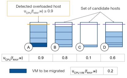
Figure 3: Case of use of VM allocation algorithm. Initial status.

4.1.1 $SO_{1}$: $min\{{\Delta}P_{Host}\}$

This policy minimizes the increment of power consumption when a VM is allocated in a host. The algorithm consolidates the VM in the server whose power consumption has the lowest increase in terms of power. The increment is calculated as the difference between the power after and before the allocation of the incoming VM. In the case of use presented in this subsection, the CPU utilization values after allocation of servers B, C and D are 1, 0.3 and 0.8 respectively. For this example, a host is considered overloaded if its CPU utilization is equal to or higher than 0.9, so host B would not be a valid candidate to host the VM. According to Figure 4, host power increment after the allocation of servers C and D is 10 W and 20 W respectively. So, the $SO_{1}$ policy chooses server C as the best candidate to host the VM, as it provides a higher CPU utilization after the allocation. This approach has been proposed by Beloglazov et al. ⁶ in their PABFD algorithm. We present this policy in this section, as we include it in our multi-objective approaches in the following sections.

4.1.2 $SO_{2}$: $min\{P_{Host}\}$

The consolidation value is the host’s power consumption. The algorithm chooses the server that presents the lowest power consumption when hosting the incoming VM. In our case of use the host power values after allocation are 170 W and 200 W respectively for servers C and D. So, the $SO_{2}$ policy chooses server C as the best candidate to host the VM. The main objective of this policy is to support the need of understanding the different contributions to power in a data center and it is available in the state-of-the-art ²⁰, ³⁹. The fact is that the global power consumption can not be reduced by minimizing local power, as the static contribution increases globally with the number of active hosts. However, this consolidation technique may be useful in some scenarios in which power capping is a necessity, enforcing a drastic reduction of server power.

4.1.3 $SO_{3}$: $min\{1/(u_{cpu}-\Delta freq)\}$

The consolidation value calculated by this approach has been proposed by the authors in previous work ³. Our proposed policy is not only aware of the utilization of the incoming VM, but also considers the impact of its allocation in terms of frequency. In our case of use, according to Figure 4, the frequency increment after the allocation of servers C and D is 0 and 0.4 respectively, so the allocation values are 1/0.3 and 1/(0.8-0.4). So, the $SO_{3}$ policy chooses server D as the best candidate to host the VM. This approach is interesting from the point of view of combining both static and dynamic contributions to global power consumption from a local perspective. The higher the CPU utilization allowed in servers, the lower the number of active hosts required to execute the incoming workload, thus reducing global static consumption. However, host’s dynamic consumption increases with frequency. As frequency increases with CPU utilization demand, we propose a compromise between increasing the $u_{cpu}$ after the allocation and reducing the frequency increment due to the incoming VM. This equation may be devised as both the $u_{cpu}$ and the frequency increment range in the same orders of magnitude.

4.1.4 $SO_{4}$: $min\{T_{mem}\}$

This consolidation approach aims to minimize the temperature of the memory as it has been demonstrated to be a key contribution to static power consumption. In our case of use, the memory temperature values after allocation are 38°C and 55°C respectively for servers C and D. So, the $SO_{4}$ policy chooses server C as the best candidate to host the VM. Moreover, this parameter also depends on the inlet temperature of the server, which impacts on the cooling power of the data center infrastructure and on the dynamic memory activity. Cooling down the computing infrastructure is needed to avoid failures on servers due to temperature, or even the destruction of components as in the case of thermal cycling and electromigration among others. Therefore, this policy may be helpful for extremely hot conditions in the outside, and also when undergoing cooling failures.

4.1.5 $SO_{5}$: $min\{\Delta freq\}$

This algorithm consolidates the VM in the server whose frequency has a lowest increase. The policy aims to minimize the increment of power consumption when a VM is allocated in a host. The increment is calculated as the difference between the frequency after and before the allocation of the VM. In our case of use, according to Figure 4, the frequency increment after the allocation of servers C and D is 0 and 0.4 respectively. So, the $SO_{5}$ policy chooses server C as the best candidate to host the VM. This consolidation technique aims to minimize the dynamic contribution to power consumption.

4.1.6 $SO_{6}$: $min\{1/u_{cpu}\}$

The consolidation value proposed in this approach maximizes the overall CPU utilization in the active host set, also constraining the number of active servers. In the case of use presented in this subsection, the CPU utilization values after allocation of servers C and D are 0.3 and 0.8 respectively. So, the $SO_{6}$ policy chooses server D as the best candidate to host the VM. In all our proposed approaches, the maximum load that can be allocated in each host is bounded by its available resources. Also, the VMs are migrated from overloaded servers according to previous workload variations. However, the possibilities of violating the SLA are high when using this specific technique. This is because workload variations in a highly loaded server may exceed the total resource capacity of the device, degrading the performance of the applications. This policy may be specially useful in scenarios with low penalties per SLA violations or if performance degradation does not have a great impact on economic or contractual issues.

4.1.7 $SO_{7}$: $min\{P_{Host}+P_{Cooling}\}$

The consolidation value is the aggregation of the host’s power consumption and the power dimensioned to cool it down avoiding thermal issues. The algorithm chooses the server that presents the lowest power IT and cooling consumption when hosting the incoming VM. In our case of use, the host and cooling aggregated power values after allocation are 187 W and 220 W respectively for servers C and D. So, the $SO_{7}$ policy chooses server C as the best candidate to host the VM. The main objective of this policy is to show the relevance of understanding the thermal contributions to power in a data center. The overall power consumption can not be reduced by minimizing local power, as the static IT contribution increases globally with the number of active hosts and the cooling power depends on IT consumption as well as on their inlet temperature needed to keep them safe. However, this consolidation technique may be useful in some scenarios in which power capping is a necessity in both IT and cooling infrastructures and when combined with variable cooling techniques.

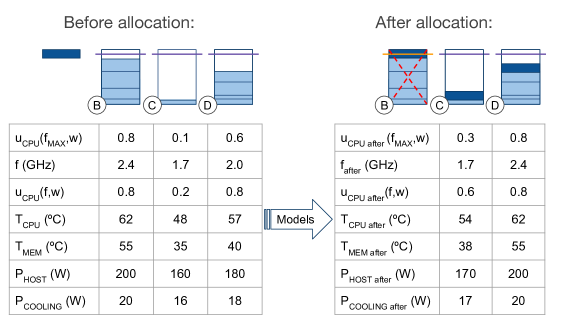
Figure 4: Case of use of VM allocation algorithm. Values before and after VM allocation.

4.1.8 $SO_{8}$: $min\{\sum|SO_{X}|\}$

This approach aims to minimize the total power consumption of the data center by combining the different parameters presented in the SO section in a single metric. In order to make the values comparable, we normalize them in the range [1,2] (according to their maximum and minimum in each range) so all the inputs take values in the same orders of magnitude. It is worth to mention that we have performed a variable standardization for every feature in order to ensure the same probability of appearance for all the variables. The algorithm consolidates the VM in the host that minimizes the summation of all the normalized parameters as seen in Equation 1. After an exhaustive analysis, the best global power results are shown for the parameter combination presented in Equation 2.

$$SO_{8} = min\{|\Delta P_{Host}|+|P_{Host}|+|1/(u_{cpu}-\Delta freq)|+|T_{mem}|+|\Delta freq|+|1/u_{cpu}|+|P_{Host}+P_{Cooling}|\}$$ (1)

$$SO_{8} = min\{|1/(u_{cpu}-\Delta freq)|+|\Delta freq|+|1/u_{cpu}|\}$$ (2)

4.2 Multi-Objective BFD-based Allocation Policies

The approaches that we present in this section also aim to minimize global power consumption from a local perspective. However, these policies do not consider one single objective to be optimized, but more than one. Multi-Objective (MO) optimizations try to simultaneously optimize several contradictory objectives. This is also useful due to the fact that, in some cases, the parameters cannot be linearly combined as they are not comparable without normalization (e.g. their orders of magnitude are very different). In all our MO policies, the VMs from VMlist are also allocated one by one in the host that minimizes the consolidation value according to the given policy. However, MO techniques offer a multidimensional space of solutions instead of returning a single value. For this kind of problems, single optimal solution does not exist, and some trade-offs need to be considered. The number of dimensions is equal to the number of objectives of the problem. Each objective of our MO strategy consists of each one of the SO consolidation values presented in Subsection 4.1. Hence, to find the solution for the allocation of a VM in a specific $Host_{i}$ from hostList, we calculate the consolidation value of all the SO policies in SOList ({$SO_{1},...,SO_{7}$}) using the SOvalue() function as can be seen in Algorithm 2. We do not include the single objective $SO_{8}$ in this calculations as its resulting value is a linear combination of the rest of SO objectives. Thus, each solution of the algorithm has the following multi-objective vector (hostVector):

$$solution_{Host_{i}}=\{\Delta P_{Host_{i}},P_{Host_{i}},1/(u_{cpu}-\Delta freq)_{i},T_{mem_{i}},\Delta freq_{i},1/u_{cpu_{i}},P_{Host_{i}}+P_{Cooling_{i}}\}$$ (3)

Then, we constrain the set of solutions to provide the ones that are in the Pareto-optimal Front (POF) paretoOptimal. This optimal subset provides only those solutions that are non-dominated by others in the entire feasible search space. This approach discards solutions that may be the optimum for a SO policy, but are dominated by other solutions that appear in MO problems. The MOvalue() function computes the objective according to the model selected from those presented in the following subsections 4.2.1 and 4.2.2. bestPlacement and bestHost are the best placement value for each iteration and the best host to allocate the VM respectively. Then, each VM in vmList will be allocated in a server that belongs to the list of hosts whose hostVector are non-dominated and have enough resources to host it. The VM is allocated in the host that has the lowest placement value. The output of this algorithm is the placement (MOPlacement) of the VMs that have to be mapped according to the MAD-MMT detection and VM selection policy. In this section, we present two MO metrics to decide a solution from the Pareto-optimal set of solutions.

Algorithm 2 MO Placement Policy

1:hostList, vmList, SOList

2:MOPlacement of VMs

3:vmList.sortDecreasingUtilization()

4:foreach vm in vmList do

5:     bestPlacement $\leftarrow$ MAX

6:     bestHost $\leftarrow$ NULL

7:     foreach host in hostList do

8:         if host has enough resources for vm then

9:              foreach SO in SOList do

10:                  hostVector.add(SOvalue())

11:              end for

12:              hostVectorSolutions.add(host, hostVector)

13:         end if

14:     end for

15:     paretoOptimal $\leftarrow$ hostVectorSolutions.getNonDominatedHostVectors()

16:     foreach host in paretoOptimal do

17:         placement $\leftarrow$ MOvalue()

18:         if placement $<$ bestPlacement then

19:              bestHost $\leftarrow$ host

20:              bestPlacement $\leftarrow$ placement

21:         end if

22:     end for

23:     if bestHost $\neq$ NULL then

24:         MOPlacement.add(vm, bestHost)

25:     end if

26:end for

27:Return: MOPlacement

4.2.1 $MO_{1}$: $min\{\sum(P_{host}+P_{Cooling})\}$

To allocate each VM, we consider the solution from the Pareto-optimal set that provides the lowest global IT and cooling power. Thus, for every solution in the POF, the algorithm calculates the $MO_{1}$ consolidation value as the power consumed by the data center considering the VM placement. Then, the VM is allocated in the host that minimizes this consolidation value.

4.2.2 $MO_{2}$: $min\{|d(solution_{Host_{i}},o)|\}$

For each solution in the POF, the algorithm calculates the Euclidean distance from the objective vector $solution_{Host_{i}}$ to the origin. Finally, the VM is allocated in the host that minimizes this distance.

4.3 Metaheuristic-based Allocation Policies

In order to compare our algorithms with non-local policies we consider a different approach. Local search methods usually fall in suboptimal regions where many solutions are equally fit. The method proposed in this section intends to help the solutions to get out from local minimums finding better solutions. Metaheuristics aim to optimize the global power consumption by simultaneously allocating all the VMs in the available host set, instead of in a sequential way as in our BFD-based algorithms. Thus, these algorithms do not only consider local power in each server but the entire IT and cooling data center consumption during the allocation.

4.3.1 Simulated Annealing: $min\{\sum(P_{Host}+P_{Cooling})\}$

The Simulated Annealing (SA) ¹⁸ is a metaheuristic based on the physical annealing procedure used in metallurgy to reduce manufacturing defects. The material is heated and then it is cooled down slowly in a controlled way, so the size of its crystals increases and, in consequence, this minimizes the energy of the system. SA is used for solving problems in a large search space, both unconstrained and bound-constrained, approximating the global optimum of a given function. This algorithm performs well for problems in which an acceptable local optimum is a satisfactory solution, and it is often used when the search space is discrete. Our version of SA proposed in this research minimizes the power consumption of the data center after the consolidation of the VM set along the infrastructure. We provide the structure of the SA allocation problem in Figure 5, where each ($VM_{i}$) is hosted in $Host_{VM_{i}}$. The size of the solution is the size of the list of VMs that have to be allocated in the system. The allocation is performed for the solution that minimizes the global data center power, considering both IT and cooling contributions. The objective function finalObjective aggregates a power objective (objectivePower) and a feasibility constraint (feasibilityConstraint) according to Equation 4.

$$finalObjective=objectivePower*(1+feasibilityConstraint)$$ (4)

Figure 5: Solution scheme for the SA algorithm.

where objectivePower is the summation of the power consumption of all the hosts and cooling for each solution. This function also incorporates penalties in the solution evaluation for those servers that are overutilized after the consolidation process in terms of CPU utilization, RAM memory or I/O Bandwidth. feasibilityConstraint is zero if the solution proposes a VM allocation for the entire set of VMs that meets all the requirements for all the hosts. Otherwise, this term is the summation of the excess of CPU, RAM and I/O Bandwidth for the entire host set and is several orders of magnitude higher than the objectivePower term. This approach reduces the probability of obtaining a solution that is not feasible in our scenario. SA algorithms are usually initialized with a random solution. Due to the large space of solutions of our problem, this approach was unable to provide feasible solutions. So, we improved our SA by initializing the first iteration with the best solution found by the SO set of algorithms ($SO_{1}$ to $SO_{8}$). This initialization ensures that the SA finds a feasible solution that is, at least, as good as the one provided by the best SO in each optimization slot. Steps 1 and 2 of our Metaheuristic Placement Policy shown in Algorithm 3 perform this initialization.

Then, the description of the problem (problemSA) is provided by this initial solution, together with the VMs in vmList that have to be placed simultaneously within the hostList set. Step 4 in Algorithm 3 provides the best solution (bestSolution) obtained by the SA. Finally, the algorithm stores the placement of all the VMs in the hosts provided by bestSolution in the output MetaheuristicPlacement. As we would like to compare our work with a metaheuristic-based global algorithm, we will use this algorithm as a baseline for the rest of local BFD-based policies.

Algorithm 3 Metaheuristic Placement Policy

1:hostList, vmList, bestSolutionSO, bestPlacementSO

2:MetaheuristicPlacement of VMs

3:bestPlacement $\leftarrow$ bestPlacementSO

4:bestObjective $\leftarrow$ bestSolutionSO

5:problemSA $\leftarrow$ problem(vmList, hostList, bestPlacement)

6:bestSolution $\leftarrow$ SimulatedAnnealing(problemSA)

7:foreach vm in bestSolution do

8:     bestHost $\leftarrow$ vm.getHost()

9:     MetaheuristicPlacement.add(vm, bestHost)

10:end for

11:Return: MetaheuristicPlacement

4.4 Metaheuristic-based SO Allocation Policies

Metaheuristics, as SA, help us to achieve a global minimization searching for the optimum, but, however, may take a higher simulation time when compared to local policies. For very complex scenarios, the time required by the SA to find the solution may exceed the time fixed for the optimization slot, making it unfeasible to use this metaheuristic during runtime. On the other hand, local policies (both SO and MO), provide fast optimizations, but their solutions may fall into suboptimal regions as they rely on local information. In this subsection we present a novel strategy to derive a global minimization from a local perspective based on modeling the global energy consumption of metaheuristic-based optimizations. Our approach is used to model a new SO policy that combines the different SO consolidation metrics presented in Subsection 4.1 in order to find a local policy that outperforms their single outcomes. By using this modeling technique, we aim to find a local, fast and light consolidation algorithm that is aware of the global relationships between the contributions to energy, not only during the allocation, but also taking into account further VM migrations.

First, we monitor the global energy values obtained during the simulation of the SA optimization. Under the same context, we run the SO simulation and monitor the global energy values and the local consolidation values for the same workload, so the optimization slots are the same. Using the optimization slots, we align the data from both sources and obtain only the optimization slots in which the SA outperforms the SO solutions in terms of global energy. This is necessary to model the improvement provided by the joint IT and cooling energy minimization, because the SA is initialized to the best SO solution (explained in Subsection 4.3.1) and in some cases the metaheuristic is not able to find a better solution. Based on these values, we model the global energy of the SA using the SO consolidation and energy values as in Equation 5. Then, we use this function to provide a $SO_{SA}$ local consolidation value for optimizing the system as done before for the regular SO policies. So, we use $SO_{SA}$ as the other SO policies, allocating the VMs of the set, one by one, in the host that offers a lowest consolidation value (as detailed in Algorithm 1). Further details regarding the implementation of this strategy are provided in Section 5.

$$SO_{SA}=E_{SA}=f(SO_{1},E_{SO_{1}},SO_{2},E_{SO_{2}},...,SO_{8},E_{SO_{8}})$$ (5)

4.5 BFD-based SO Dynamic selection Allocation Policy

The SO strategies provided in this research offer different allocation policies from a local perspective. However, the Cloud computing context presented in this research shows a very high variability during runtime in terms of resource demand. According to the SO approaches, in each optimization slot, the system only has the information of a specific instantaneous state and local policies are not aware of the variability during runtime. The approach that we present in this section also aims to minimize global power consumption from a local perspective but is intended to adapt the system optimization to the dynamism of the Cloud environment. Therefore, this policy does not consider only one consolidation value, but the complete set of values offered by all the SO approaches in this research. The SO Dynamic Selection approach (DynSO) allocates the set of VMs using the SO policy that minimizes the overall IT power in each time slot.

$$SO\in\{SO_{1},...,SO_{n},...,SO_{N}\}$$ (6)

We define $SOList$ as $\{SO_{1},...,SO_{8},SO_{SA}\}$, incorporating all the SO policies provided in this research. Algorithm 4 presents the implementation for this allocation policy. In the first iteration, the algorithm evaluates the final global power consumption ($GlobalPower_{n}$) provided by the allocation of the entire set of VMs in VMList, as in Algorithm 1, using the consolidation value of the first SO in SOList ($SO_{n}=SO_{1}$). The obtained placement map (tentativeSOPlacement) is used to get the global power provided by this allocation policy (GlobalPowerSO), using the function getSOGlobalPower. Then, the algorithm stores the global power, and the SO used in the PowerSO table. The same calculations are done for the rest of $SO_{n+1}$ until all the N-dimensioned set of SOs is covered obtaining the complete table PowerSO shown in Figure 6.

Figure 6: Dynamic selection of the best SO policy.

Finally, the functions getSOMinPowerAfterAlloaction() and getTentativeSOPlacement() provide the minimum global power ($GlobalPower_{min}$) and the corresponding SO for which it has been obtained $SO_{Pmin}$. So, the $SO_{Pmin}$ is used for allocating the VMs in the current time slot using Algorithm 1.

Algorithm 4 Dynamic SO Placement Policy

1:hostList, vmList, SOList

2:$SO_{Pmin}$

3:vmList.sortDecreasingUtilization()

4:foreach SO in SOList do

5:     foreach vm in vmList do

6:         bestPlacement $\leftarrow$ MAX

7:         bestHost $\leftarrow$ NULL

8:         foreach host in hostList do

9:              if host has enough resources for vm then

10:                  placement $\leftarrow$ SOvalue()

11:                  if placement $<$ bestPlacement then

12:                       bestHost $\leftarrow$ host

13:                       bestPlacement $\leftarrow$ placement

14:                  end if

15:              end if

16:         end for

17:         if bestHost $\neq$ NULL then

18:              tentativeSOPlacement.add(vm, bestHost)

19:         end if

20:     end for

21:     GlobalPowerSO $\leftarrow$ getSOGlobalPower(tentativeSOPlacement)

22:     PowerSO.add(SO,GlobalPowerSO)

23:end for

24:$GlobalPower_{min}$ $\leftarrow$ PowerSO.getSOMinPowerAfterAlloaction()

25:$SO_{Pmin}$ $\leftarrow$ PowerSO.getTentativeSOPlacement($GlobalPower_{min}$)

26:Return: $SO_{Pmin}$

5 Modeling Metaheuristic-based SO Allocation Objectives

In this section we aim to obtain an expression that defines the energy behavior of our SA allocation algorithm using local optimizations. For this purpose, we model the global energy consumption at each optimization slot for the metaheuristic ($Energy_{SA}$) using the parameters of the different SO described in Section 4. The conducted experiments have the same configuration as the ones described in Subsection 7.1. First, we run the workload using the SA optimization algorithm for VM allocation and, after each time slot, we collect the global energy consumption $E_{SA}$. Under the same context, we run the workload using each $SO_{n}$ algorithm and, after each optimization slot we monitor: i) the consolidation value normalized in the range [1,2] ($|SO_{n}|^{2}_{1}$), and ii) the total energy consumption of the infrastructure after the consolidation process is completed ($E_{SO_{n}}$). Considering the global energy of the entire data center helps us to incorporate in the optimization the knowledge not only from the IT and cooling contributions but also from the contributions of the VM migrations that are needed after the allocation to avoid underloaded situations. In this work we use a SA configured as in Subsection 7.1.3. For SA samples, we separate the entire monitored data into a training and a testing data set. The data set used for this modeling process consists of the samples collected during the simulation of only the first 24 hours of the Workload 1. Also, we only use those samples in which the SA outperforms the SO policies in terms of energy, as the SA not always perform better than the SO strategies because it could provide worse final solutions to get out from local minima. We train the models, using the classic regression lsqcurvefit from MATLAB, inferring the expressions shown in Equation 7, where $|SO_{3}|^{2}_{1}$ and $|SO_{6}|^{2}_{1}$ are the normalized consolidation values obtained for local optimizations $SO_{3}$ and $SO_{6}$ respectively.

$$SO_{SA} = E_{SA}=0.1603\cdot|SO_{3}|^{2}_{1}\cdot E_{SO_{3}}+0.7724\cdot|SO_{6}|^{2}_{1}\cdot E_{SO_{6}}+0.0102$$ (7)

The fitting is shown in Figures 7 and 8 for training and testing respectively. For the SA energy, $E_{SA}$, we obtain an average error percentage of 3.05% and 2.87% for training and testing. Finally, we use this expression to calculate the consolidation value used in $SO_{SA}$.

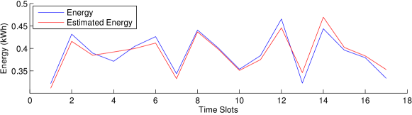
Figure 7: Modeling fitting for $SO_{SA}$ using Simulated Annealing samples.

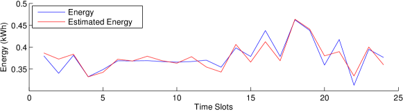
Figure 8: Testing modeling for $SO_{SA}$ using Simulated Annealing samples.

For our model we obtain a mean error between the estimated energy and the real trace of $8.84\cdot 10^{-7}$ kWh and a standard deviation of 0.0144 kWh. Figure 9 shows the power error distribution for this model, where it can be seen that the error in terms of power of about the 68% of the samples may range from -0.0144 to 0.0144 kWh.

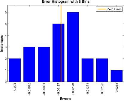
Figure 9: Power error distribution for our $SO_{SA}$ model.

6 Cooling strategy based on VM allocation

The power needed to cool down the servers, thus maintaining a safe temperature, is one of the major contributors to the overall data center budget. Many of the reliability issues and system failures in a data center are given by the adverse effects due to hot spots that may also cause an irreversible damage in the IT infrastructure. However, controlling the set point temperature of the data room is still to be clearly defined and represents a key challenge from the energy perspective. This value is often chosen for the worst case scenario (all devices running consuming maximum power), and based on conservative suggestions provided by the manufacturers of the equipment, resulting in overcooled facilities. In this section we present a novel cooling strategy based on the temperature of the system’s devices due to VMs’ allocation that can be seen in Algorithm 5. Our cooling strategy, called VarInlet, aims to find the highest cooling set point of the CRAC units that ensures a safe operation for the whole data center infrastructure under variable workload conditions. Inside the physical machine, the CPU is the component that presents the highest temperatures and this parameter depends on both the inlet temperature and the CPU utilization (utilization). So, the CPU temperature will limit the highest value for the inlet temperature of the host (maxInletTemperature) in order to operate in a safe range (lower than maximumSafeCPUTemperature) avoiding thermal issues. Depending on the VMs’ distribution and the server location, we define a maximum cooling set point (maxCoolingSetPoint) for each host that ensures that its maximum inlet temperature is not exceeded so the CPU temperature is safe. Finally the cooling set point is set to the lowest value within the maxCoolingSetPoint for all the servers, thus guaranteeing that the infrastructure operates below the maximumSafeCPUTemperature in each optimization slot.

Algorithm 5 Cooling strategy

1:hostList maximumSafeCPUTemperature

2:cooling

3:foreach host in hostList do

4:     utilization $\leftarrow$ host.getUtilization()

5:     maxInletTemperature $\leftarrow$ host.getMaxInletTemperature(utilization, maximumSafeCPUTemperature)

6:     maxCoolingSetPoint $\leftarrow$ host.getMaxCoolingSetPoint(maxInletTemperature)

7:     hostCooling.add(maxCoolingSetPoint)

8:end for

9:globalMaxCoolingSetPoint $\leftarrow$ hostCooling.getMin()

10:cooling.setCoolingSetPoint(maxCoolingSetPoint)

11:Return: cooling

7 Performance Evaluation

In this section, we present the impact of our proposed optimization strategies in the energy consumption of the data center, including both IT and cooling contributions. As it is difficult to replicate large-scale experiments in a real data center infrastructure, thus maintaining experimental system conditions, we have chosen the CloudSim 2.0 toolkit ⁷ to simulate a IaaS (Infrastructure as a Service) Cloud computing environment. This simulator has been successfully used for VM allocation in Cloud computing at different levels, taking into account multiple objectives and constraints, and using both heuristic and metaheuristic approaches ¹⁵, ¹⁴. For this work, we have provided DVFS (Dynamic Voltage and Frequency Scaling) management and thermal-awareness to the CloudSim simulator. Moreover, the temperature of servers’ inlet, memory devices and CPUs vary depending on the workload distribution and on the resource demand. We incorporate these dependence by including different thermal models. Also our frequency and thermal-aware server power model has been included. Finally, in order to obtain temperature and power performance, we have also incorporated memory and disk usage management. Our simulations run on a 64-bit Ubuntu 14.04.5 LTS operating system running on an Intel Core i7-4770 CPU @3.40GHz ASUS Workstation with four cores and 8 GB of RAM. Experiments are configured according to the following considerations.

7.1 Experimental Setup

We conduct our experiments using real data from the Bitbrains service provider. This workload has the typical characteristics of Cloud computing environments in terms of variability and scalability ³⁸. Our data set contains performance metrics of 1,127 VMs from a distributed data center. It includes resource provisioning and resource demand of CPU, RAM and disk as well as the number of cores of each VM with a monitoring interval of 300 seconds. These parameters define the heterogeneous VM instances available for all the simulations. We split the data set into three workloads that provide three scenarios with different CPU variability. Each scenario represents one week of real traces from the Bitbrains Cloud data center. As can be seen in Figure 10, Workloads 1 to 3 present decreasing aggregated CPU utilization variability of 568.507%, 284.626% and 143.603% respectively.

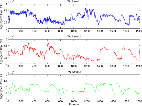
Figure 10: One-week workloads with different CPU utilization variability.

The simulation consists of a data center of 1200 hosts modeled as a Fujitsu RX300 S6 server based on an Intel Xeon E5620 Quad Core processor @2.4GHz, RAM memory of 16GB and storage of 1GB, running a 64bit CentOS 6.4 OS virtualized by the QEMU-KVM hypervisor. During the simulations, the number of servers will be significantly reduced as oversubscription is enabled. The proposed Fujitsu RX300 S6 server is based on an Intel Xeon E5620 processor operating at $f_{m2}=1.73$ GHz, $f_{m3}=1.86$ GHz, $f_{m4}=2.13$ GHz, $f_{m5}=2.26$ GHz, $f_{m6}=2.39$ GHz and $f_{m7}=2.40$ GHz. For optimization purposes, we have simulated all our algorithms under the frequency constraints of our ad-hoc DVFS-performance aware governor proposed in our previous work ³, as it has been demonstrated to give further energy improvements without affecting SLA. Moreover, maximum CPU temperature is constrained to take values that are lower or equal to 65$\degree$ C for reliability purposes. Also server’s inlet is limited to a 30$\degree$ C upper bound, to avoid fan failures.

7.1.1 Power and Thermal Models

In this subsection, we present the different models referred in our previous work, and also two novel ones derived for this research. To estimate the energy consumed by the IT infrastructure, we use our DVFS and thermal aware server power model defined in our previous research ⁴.

$$P_{\mathrm{Fujitsu}}(k,w) = 3.32\cdot V^{2}_{\mathrm{DD}}(k)\cdot f_{op}(k)\cdot u_{\mathrm{CPU}}(k,w)+1.63\cdot 10^{-3}\cdot T^{2}_{\mathrm{MEM}}+4.88\cdot 10^{-11}\cdot FS^{3}$$ (8)

$$E_{\mathrm{Fujitsu}}(k,w) = P_{\mathrm{Fujitsu}}(k,w)\cdot t$$ (9)

$$f_{op}(k) \in \{1.73,1.86,2.13,2.26,2.39,2.40\}$$ (10)

$$E_{boot} = 13.514\cdot 10^{-3}kW\cdot h$$ (11)

Equation 8 shows the power consumption of the Fujitsu server, where $V_{\mathrm{DD}}(k)$ is the CPU supply voltage and $f_{op}(k)$ is the working frequency in GHz of the server in a specific k DVFS mode. $u_{\mathrm{cpu}}(k,w)$ is the averaged CPU percentage utilization running a workload w at the k DVFS mode. $T_{\mathrm{mem}}$ defines the memory temperature in Kelvin and FS describes the fan speed in RPM. This model achieves a testing error of 4.46% when comparing power estimation to real measurements of the actual power in Cloud applications. The energy consumption is obtained using Equation 9 where t defines the time in which the energy value is required. In our research, the time slots are defined as each time an optimization is performed in order to consolidate a set of VMs into a set of candidate hosts. We use a value of t of 300 seconds to match the workload traces provided by BitBrains. The operating frequencies set (in GHz) is provided in 10. In this work, we assume that servers are powered on and off when needed, so we take into account the booting energy consumption required by a server to be fully operative as shown in Equation 11.

As our power model shown in Equation 8 depends on the memory temperature, for this research, we present a novel temperature model for the memory device. The temperature of the memory device in a server depends on several factors both internal and external to the physical machine. The utilization of the memory subsystems, the inlet temperature of the host and the fan speeds are potential contributors to memory temperature that have to be taken into account. In order to gather the real data during runtime, we monitor the system using different hardware and software resources. collectd monitoring tool is used to collect the values taken by the system in order to monitor $u_{MEM}$. Memory and CPU temperatures and fan speed are monitored using on board sensors that are consulted via the IPMI software tool. Inlet temperature is collected using external temperature sensors. Finally, room temperature has been modified during run-time in order to find the dependence with the inlet temperature.

In this research, a synthetic workload is used to stress specifically the memory resources, increasing the range of possible values of the considered variables. Therefore, our model may be adapted to estimate different workload characteristics and profiles. We run a version of $RandMem$ (modified to access random memory regions individually) onto 4 parallel Virtual Machines that have been provisioned to the available computing resources of the server. Then the samples are separated into a training and a testing data set. After training, we obtain the model shown in Equation 12, where $T_{mem}$ is the memory temperature, $U_{mem}$ the memory utilization, $T_{inlet}$ the inlet temperature of the server, $k_{1}=0.9965$ and $k_{2}=2.6225$. Then, we evaluate the quality of the thermal model using the testing data set in order to verify the reliability of the estimation. For our data fitting, we obtain an average error percentage of 0.5303% during training and 0.5049% for testing. These values have been obtained using Equation 13.

$$T_{mem} = k_{1}\cdot T_{inlet}+k_{2}\cdot ln(U_{mem}^{2})$$ (12)

$$e_{AVG} = \sqrt{\frac{1}{N}\cdot\sum_{n}{\Big{(}\frac{|T_{mem}(n)-\widehat{T_{mem}}(n)|\cdot 100}{T_{mem}(n)}\Big{)}}^{2}},1\leq n\leq N$$ (13)

Finally, for our thermal model we obtain a mean error between the estimated temperature and the real measurement of $8.54\cdot 10^{-4}$ K and a standard deviation of 2.02 K. Figure 11 shows the error distribution for this model. According to this, we can conclude that the error in terms of temperature of about the 68% of the samples ranges from -2.02 to 2.02 K. In Figure 12, the fitting of our thermal model is provided.

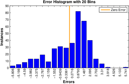
Figure 11: Temperature error distribution for our memory model.

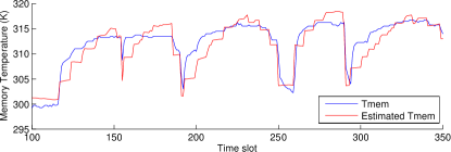
Figure 12: Modeling fitting for the memory temperature.

On the other hand, the CPU presents the highest temperatures inside the physical machine, so its temperature will limit the highest value for inlet temperature in order to operate in a safe range, while avoiding thermal issues. Thus, we follow the same approach in order to model the CPU temperature of the server. This parameter depends on both the inlet temperature and the CPU utilization ($u_{CPU}$). After training, we obtain the model shown in Equation 14, where $T_{cpu}$ is the CPU temperature, $U{cpu}$ its utilization, $k_{1}=1.052$ and $k_{2}=19.845$. Our model presents average error percentages of 0.64% and 0.84% during training and testing respectively.

$$T_{cpu} = k_{1}\cdot T_{inlet}+k_{2}\cdot U_{cpu}$$ (14)

Finally, we obtain a mean error between the estimated temperature and the real measurement of 0.0026 K and a standard deviation of 2.683 K. Figure 13 shows the error distribution for this model, where the error in terms of temperature of about the 68% of the samples ranges from -2.68 to 2.68 K. In Figure 14, the fitting of our thermal model is provided.

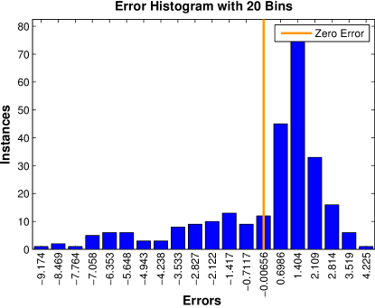
Figure 13: Temperature error distribution for our CPU model.

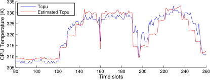
Figure 14: Modeling fitting for the CPU temperature.

Disk power consumption is modeled according to the work proposed by Lewis et al. ²¹, as can be seen in Equation 15, where $Disk_{r}$ and $Disk_{w}$ are the read and write throughputs. We define cooling energy model, shown in Equation 16, as in the research presented by Moore et al. ²⁷. The COP depends on the inlet temperature of the servers’ $T_{inlet}$.

$$P_{Disk} = 3.327\cdot 10^{-7}\cdot Disk_{r}+1.668\cdot 10^{-7}\cdot Disk_{w}$$ (15)

$$E_{Cooling} = E_{IT}/COP=(P_{IT}\cdot t)/COP$$ (16)

$$E_{IT} = (P_{Fujitsu}+P_{Disk})\cdot t$$ (17)

$$COP = 0.0068\cdot T_{inlet}^{2}+0.0008\cdot T_{inlet}+0.458$$ (18)

7.1.2 Dynamic Consolidation considerations

In all our scenarios we allow online migration, where VMs follow a straightforward load migration policy. Thus, migrations have an energy overhead because, during the migration time, two identical VMs are running, consuming the same power in both servers. Performance degradation occurs when the workload demand in a host exceeds its resource capacity. Our dynamic consolidation strategy first chooses which VMs have to be migrated in each server of the data center. For this purpose, we use the adaptive utilization threshold based on the Median Absolute Deviation (MAD) of the CPU and the Minimum Migration Time (MMT) algorithm provided by Beloglazov et al. ⁶. Then, the VM allocation is performed according to the optimization algorithms provided in Section 4. In this work we allow oversubscription in all the servers so, the total resource demand may exceed their available capacity. If the VMs in a host simultaneously request their maximum performance, this situation may lead to performance degradation due to host overloading. When overloading situations are detected using the MAD-MMT technique, VMs are migrated to better placements according to the different proposed algorithms. This procedure creates a performance degradation due to the migrations required. In this research, we determine SLA violations ($SLA_{violation}$), as the metric provided by CloudSim, further explained in the research proposed by Beloglazov et al. ⁶. This metric combines the performance degradation due to both host overloading and migrations, and would help us to monitor the SLA provided by our optimization system.

7.1.3 SA Configuration

In this work we use the SA provided by the HEuRistic Optimization (HERO) library of optimization algorithms. We executed 32 simulations to determine the maximum number of iterations, as well as the value of k. After these tests we observed that the best solution was never improved beyond 100000 iterations, independently of the value of k. k is a weight used to compute the probability of changing the state to a new solution. $k=0.5$ offered the best solutions overall. The probability of changing the state when the new solution worsens the current solution depends on $e^{-(x/k)}$ so, for $k=0.5$, it results on $e^{-(2x)}$ meaning that the probability of changing the state is reduced in such exponential factor. This makes sense when the initial solution is “good” (we set the initial solution to the best found by the SO policies) because an improvement in energy can be reached with small number of permutations of virtual machines. Additionally, we had a hard time constraint for performance purposes, for instance, the maximum execution time of the SA algorithm should not exceed 300 seconds, and 100000 iterations safely entered in that time window. Finally, we modified the basic implementation of the HERO library to facilitate the selection of the best-so-far solution, which is not included by default.

7.2 Baselines

In this research, we compare our proposed technique against a heuristic, a metaheuristic, and a recent state-of-the-art algorithm. As heuristic, we select a BFD-based algorithm due to its light implementation in terms of execution time and complexity, still being powerful enough to tackle optimization problems like the one described; as metaheuristic, we select an optimizer based on gradient descent due to its global minimization capabilities. According to the state-of-the-art that we present in Section 2, we would like to compare our proposed algorithms with a heuristic. The PABFD approach, proposed by Beloglazov et al. ⁶, is used as our BFD-based heuristic baseline. Moreover, this BFD algorithm is single-objective and provides a local optimization, so it is fast and light to be used during run-time. This algorithm is referred in many recent publications ¹⁰, ¹⁷, ⁴⁰, ²⁵, ²⁸, ³⁵, ³⁴, and it is also included in the open source version of CloudSim 2.0. The second baseline is an in-house simulated annealing approach. This algorithm is single-objective and provides a global optimization of the data center energy consumption for both IT and cooling contributions. We have enhanced the SA, initializing the algorithm to the best solution found by the SO set of algorithms. This initialization ensures that the SA finds a feasible solution that is, at least, as good as the one provided by the best SO in each optimization slot. Both PABFD and SA have been explained thoroughly in Sections 4.1.1 and  4.3.1, as they have been used as objectives to define our multi-objective policies ($MO_{1}$ and $MO_{2}$) and to model our metaheuristic-based single-objective approach ($SO_{SA}$) respectively. Finally, we include the SWFDVP (Second worst fit decreasing VM placement) algorithm as baseline, which has been recently proposed by Chowdhury et al. ¹⁰. This single-objective BFD policy is based on the almost worst fit decreasing technique and aims to allocate a VM in the bin that provides the second minimum empty space. More in detail, the objective of the SWFDVP algorithm is to maximize the power increment due to the allocation of a VM within a set of hosts, and select the host that provides the second best solution. This baseline helps us to compare our work with a real-time state-of-the-art research.

7.3 Experimental results

To obtain a preliminary evaluation of the performance of the different VM allocation policies, we have simulated one day of our Workload 1 from Bitbrains using the proposed strategies presented in Section 4 for a fixed inlet temperature of 291K. On the one hand, the simulation time when using the SO approaches ($SO_{1-8}$, $SO_{SA}$, and DynSO) ranges from 8 to 12 minutes. This parameter for MO approaches is around 15 minutes, being in the same order of magnitude. On the other hand, the metaheuristic-based SA has a simulation time that is 60 times higher than the complete simulation time of SO policies. Also, for SA, there exist some optimizations that take more time than the time fixed for the optimization slot (300 s), making it unfeasible to use this metaheuristic during runtime. The energy results provided by the selected algorithms are shown in Figure 15. Also, Table 1 shows the numerical results of the additional metrics considered.

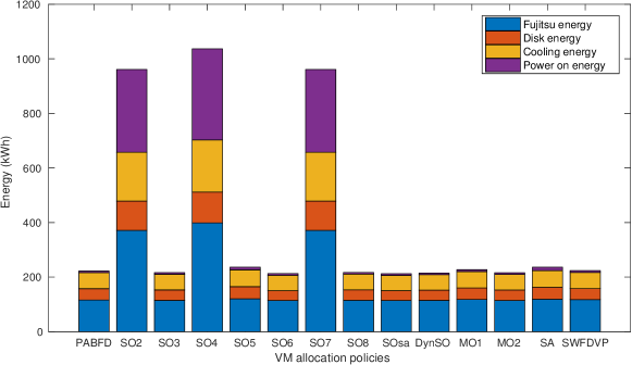
Figure 15: Contributions to data center energy per VM allocation strategy for 1 day of Workload 1

Table 1: Performance metrics per VM allocation strategy for 1 day of Workload 1

Algorithm	IT Energy	Cooling Energy	Power-on	Power-on Energy	Migrations	Average SLA	Final Energy
	(kWh)	(kWh)	events	(kWh)	events	$\cdot 10^{-4}$ (%)	(kWh)
PABFD $(SO_{1})$	157.62	58.91	309	5.80	42545	18.43	222.32
$SO_{2}$	478.54	178.85	16194	303.74	116044	11.66	961.13
$SO_{3}$	153.15	57.24	335	6.28	36711	18.28	216.67
$SO_{4}$	511.60	191.21	17792	333.71	125807	11.89	1036.52
$SO_{5}$	165.12	61.71	524	9.83	45044	18.36	236.66
$SO_{6}$	150.43	56.22	336	6.30	35619	19.29	212.95
$SO_{7}$	478.54	178.85	16194	303.74	116044	11.66	961.13
$SO_{8}$	153.54	57.38	334	6.26	37376	18.28	217.19
$SO_{SA}$	150.20	56.14	333	6.25	36983	19.50	212.58
$DynSO$	152.15	56.86	326	6.11	36126	18.71	215.13
$MO_{1}$	160.41	59.95	367	6.88	40342	18.15	227.25
$MO_{2}$	152.86	57.13	331	6.21	37690	18.62	216.20
$SA$	162.95	60.90	662	12.42	50540	18.34	236.27
SWFDVP	157.95	59.03	369	6.92	39077	18.51	223.90

For $SO_{2}$, $SO_{4}$ and $SO_{7}$, the power or temperature of each server is minimized locally resulting in a higher energy consumption due to an increase in the number of active hosts. These algorithms spread the workload as much as possible through the candidate host set as they intend to reduce only the dynamic contribution, which depends on the workload requirements. So, the lower the servers’ load, the better for reducing dynamic power consumption locally, thus increasing the global IT contribution as these policies are not aware of their impact on the rest of the infrastructure. Then, after allocating those VMs incoming from overloaded servers, in the next iteration, the algorithm constrains the active server set by migrating VMs from underutilized hosts if possible. So, these algorithms present a higher number of migrations.

Moreover, the energy consumption of both $SO_{5}$ and SA policies is above the average due to a higher number of VM migrations and power on events, performed to find the best data center configuration in each optimization slot. This is due to their trend towards allocating part of the workload in underutilized servers. In the case of $SO_{5}$, this situation occurs because, when servers present an utilization below 72% (equivalent utilization for 1.73GHz that is the lowest available frequency), their frequency increment is zero. On the other hand, for the SA algorithm, the optimization value is highly penalized when the solutions include overloaded servers. So, underutilized servers are preferred when the algorithm does not find a minimum. Our results show that $SO_{3}$ and $SO_{6}$ are the best simple-SO optimization policies. This outcome is consistent with the high idle consumption of the Fujitsu’s server architecture, so reducing the active servers’ set by increasing CPU utilization is a major target to improve energy efficiency. The multi-objective strategies that we present in this research also outperform the baseline, where $MO_{2}$ is more competitive in terms of energy.

The $SO_{SA}$ strategy shows the lowest total consumption value, providing energy savings of 4.38%, 10.02% and 5.06% on the global power budget when compared with our baselines PABFD, SA and SWFDVP respectively. This is translated into a reduction of 9.74 kWh, 23.69 kWh and 11.32 kWh as this novel technique also incorporates global information regarding the effect of allocation on future VM migrations. This local approach takes advantage of global knowledge from joint IT and cooling viewpoint thus outperforming other strategies for highly variable workloads. The DynSO policy, which dynamically sets the best SO during runtime, also reduces power significantly, but does not achieve the best result in terms of energy consumption. This is because, local policies may offer better consolidation values for the server scope but do not consider the impact on the data center as a whole once the allocation is performed (e.g. future migrations). On the other hand, the $SO_{SA}$ provides the best results in this scenario. This novel approach may not provide the best consolidation value during local calculations, but is the one that best describes the energy behavior of the entire infrastructure, considering also future migrations. Moreover, the SLA is maintained for all the tests, where a higher increment of $1.07\cdot 10^{-4}\%$ is detected.

After this proof of concept, we use all the different VM allocation policies provided in Section 4 to optimize the power consumption of our proposed data center infrastructure under several workload and cooling conditions. In this work we propose the optimization of 9 scenarios, running the three different 7 days-workload profiles shown in Figure 10 and applying three different cooling strategies. The cooling policies used in this research are: i) 291K fixed setpoint temperature (found in traditional data centers), ii) 297K fixed setpoint temperature (found in new data center infrastructures) and iii) our VarInlet cooling strategy provided in Section 6. According to our problem, the number of VMs to allocate is numVMs=1127 and the number of hosts numHosts=1200. BFD-based SO and MO policies ($SO_{1}$ to $SO_{8}$, DynSO, $SO_{SA}$, $MO_{1}$ and $MO_{2}$) are deterministic approaches with a space of solutions of numVMs*numHosts, so all the executions provide the same result. For this reason we run each of them once. On the other hand, the SA is a metaheuristic that provides different solutions that are highly dependent with the initial random solution. In our proposed SA, the initial solution is deterministic, as it is always initialized to the best solution provided by the set of SO policies, thus limiting its randomness. However, the computing time of our SA scenario is around 3-4 days due to the increased space of solutions, $numHosts^{numVMs}$ in this case. The high run time makes it difficult to run the SA scenario for a high number of executions, so the set of executions is not extensive enough to provide meaningful statistics. For these reasons, we decided to run each SA scenario only once.

First, we optimize Workload 1, which is the workload that presents the higher instantaneous variability, for fixed cooling inlets of 291 K and 297 K, and for our variable inlet cooling strategy (VarInlet). We obtain the results provided in Table 2 in terms of final energy consumption, average SLA and number of migrations.

Table 2: Energy, SLA and Migration metrics per inlet temperature and allocation policy for workload 1.

Policy	Energy (kWh)			Average SLA ($\cdot 10^{-4}$ %)			Migrations ($\cdot 10^{3}$)
	291K	297K	VarInlet	291K	297K	VarInlet	291K	297K	VarInlet
PABFD	1178.41	1089.27	1034.20	20.76	20.98	21.04	200.8	202.2	203.2
$SO_{2}$	5256.76	4718.89	4594.32	11.97	11.94	11.88	647.4	647.7	654.1
$SO_{3}$	1159.07	1059.19	1018.19	20.60	20.60	20.60	190.2	190.2	190.2
$SO_{4}$	5725.25	5207.93	4990.10	11.87	11.87	11.88	766.6	766.6	772.2
$SO_{5}$	1247.97	1139.50	1094.45	20.15	20.15	20.15	217.5	217.5	217.5
$SO_{6}$	1157.61	1057.85	1016.91	20.90	20.90	20.90	189.1	189.1	189.1
$SO_{7}$	5256.76	4718.89	4594.32	11.97	11.94	11.88	647.4	647.7	654.1
$SO_{8}$	1161.44	1061.33	1020.22	20.31	20.31	20.31	192.5	192.5	192.5
$SO_{SA}$	1152.13	1052.93	1012.30	20.84	20.84	20.84	187.9	187.9	187.9
$DynSO$	1164.30	1055.83	1020.59	20.56	20.61	20.56	190.8	189.0	192.9
$MO_{1}$	1199.55	1090.12	1047.56	20.01	20.31	19.94	198.0	199.0	201.0
$MO_{2}$	1159.39	1059.45	1018.42	20.62	20.62	20.62	191.7	191.7	191.7
$SA$	1293.51	1178.35	1130.98	19.94	19.54	19.80	244.9	241.3	244.6
SWFDVP	1193.87	1092.76	1051.76	20.60	21.11	20.44	188.4	190.9	185.3

Figure 16 shows the different contributions to final energy per VM allocation policy for the different cooling strategies. As inlet temperature rises, the IT power consumption is increased due to power leakage (see IT 291K, IT 297K and IT VarInlet at the bottom of each stacked column). However, cooling power is reduced with increasing temperatures due to a higher cooling efficiency (shown in Cooling 291K, Cooling 297K and Cooling VarInlet in the middle of each stacked column). The savings performed by higher cooling set points outperform the IT power increments, thus resulting in more efficient scenarios for all the proposed allocation strategies. The energy needed to power on the servers when it is required by the allocation policies is shown as Power on 291K, Power on 297K and Power on VarInlet respectively for the three cooling strategies. For the three scenarios running Workload 1, only by applying our VarInlet cooling strategy provides additional energy savings of 3.78% and 12.38% in average when compared with fixed cooling at 297 K and 291 K respectively for all the allocation policies.

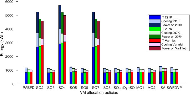
Figure 16: Contributions to data center energy per VM allocation strategy for Workload 1

Figure 17 shows the total energy and average SLA percentage comparison for those strategies that outperform the PABFD baseline, which is the baseline that performs better in this scenario in terms of energy. $SO_{SA}$, $SO_{6}$, $SO_{3}$, $MO_{2}$ and DynSO allocation policies offer better results, in terms of energy savings, when compared to our global baseline SA and our local baselines PABFD and SWFDVP. These policies, when combined with VarInlet strategy, provide savings, of 13.67% and 21.35% in average with respect to SA at 297 K and 291 K respectively. Maximum savings are found of up to 14.09% and 21.74% respectively for our VarInlet-$SO_{SA}$ combined strategy. When compared with the local baseline PABFD, these allocation policies provide average savings of 6.61% and 13.67% at 297 K and 291 K respectively, and maximum savings of up to 7.07% and 14.10% for $SO_{SA}$. Finally, comparing the results with the SWFDVP baseline, average savings of 6.91% and 14.79 % and maximum savings of 7.33 % and 15.21% (for $SO_{SA}$) are found.

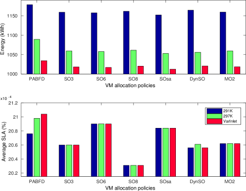
Figure 17: Data center energy and SLA per VM allocation strategy for Workload 1

In our three following scenarios we optimize Workload 2, which presents medium instantaneous variability. We obtain the energy consumption, average SLA and migration results provided in Table 3.

Table 3: Energy, SLA and Migration metrics per inlet temperature and allocation policy for workload 2.

Policy	Energy (kWh)			Average SLA ($\cdot 10^{-4}$ %)			Migrations ($\cdot 10^{3}$)
	291K	297K	VarInlet	291K	297K	VarInlet	291K	297K	VarInlet
PABFD	1033.75	949.09	912.18	18.84	18.67	18.58	119.3	126.0	123.0
$SO_{2}$	3712.18	3422.65	3278.08	11.15	11.11	11.21	564.2	579.4	570.9
$SO_{3}$	1022.49	935.02	899.36	18.43	18.43	18.43	121.7	121.7	121.7
$SO_{4}$	4562.67	4142.05	3978.78	11.00	11.00	11.01	751.5	751.5	761.0
$SO_{5}$	1081.89	988.79	950.59	18.11	18.11	18.11	136.0	136.0	136.0
$SO_{6}$	1015.27	928.55	893.27	18.51	18.51	18.51	120.8	120.8	120.8
$SO_{7}$	3712.18	3422.65	3278.08	11.15	11.11	11.21	564.2	579.4	570.9
$SO_{8}$	1024.57	936.92	901.17	18.46	18.46	18.46	120.3	120.3	120.3
$SO_{SA}$	1016.71	929.82	894.48	18.54	18.54	18.54	119.3	119.3	119.3
$DynSO$	1027.06	939.13	903.27	18.24	18.24	18.24	118.9	118.9	118.9
$MO_{1}$	1032.37	945.82	913.50	18.21	18.16	18.21	125.0	121.8	122.6
$MO_{2}$	1024.80	937.07	901.30	18.28	18.28	18.28	121.5	121.5	121.5
$SA$	1122.67	1026.40	985.68	18.34	18.12	18.06	160.1	163.3	161.6
SWFDVP	1055.37	967.99	931.64	18.36	18.36	18.85	118.3	120.1	120.8

In Figure 18 , the same trend towards power and temperature is shown as in Workload 1 scenarios. Savings obtained by increasing cooling set points also outperform IT power increments, thus resulting in more efficient scenarios for all the proposed allocation strategies. For this scenario, only our VarInlet cooling strategy provides additional energy savings of 3.88% and 12.00% in average, when compared with fixed cooling at 297 K and 291 K respectively, for all the allocation policies.

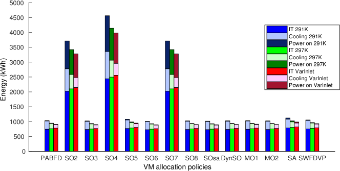
Figure 18: Contributions to data center energy per VM allocation strategy for Workload 2

Figure 19 shows the energy and average SLA percentage comparison for those strategies that outperform the baseline PABFD, which is the baseline that performs better in this scenario, in terms of energy, where SLA is maintained. As in the Workload 1 scenarios, $SO_{SA}$, $SO_{6}$, $SO_{3}$, $MO_{2}$ and DynSO allocation policies offer the best results, in terms of energy savings, when compared to our baselines SA, PABFD and SWFDVP. These policies, when combined with VarInlet strategy, provide average savings of 12.48% and 19.99% with respect to SA at 297 K and 291 K respectively, and maximum savings of up to 12.97% and 20.43% respectively for $SO_{6}$. These policies, when compared with PABFD provide average savings of 5.34% and 13.09% at 297 K and 291 K respectively, and maximum savings of up to 5.88% and 13.59% respectively for $SO_{6}$. Comparing the results with the SWFDVP baseline, average savings of 7.20% and 15.25 % and maximum savings of 7.72 % and 15.36% (for $SO_{6}$) are found.

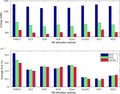
Figure 19: Data center energy and SLA per VM allocation strategy for Workload 2

Finally, we optimize Workload 3, which presents the lowest instantaneous variability. For this optimization scenarios, we obtain the energy consumption, average SLA and migration results provided in Table 4.

Table 4: Energy, SLA and Migration metrics per inlet temperature and allocation policy for workload 3.

Policy	Energy (kWh)			Average SLA ($\cdot 10^{-4}$ %)			Migrations ($\cdot 10^{3}$)
	291K	297K	VarInlet	291K	297K	VarInlet	291K	297K	VarInlet
PABFD	855.52	786.93	759.02	15.68	15.77	15.74	64.4	63.2	67.5
$SO_{2}$	2715.34	2505.51	2381.12	10.44	10.49	10.46	467.9	477.7	466.9
$SO_{3}$	852.66	781.12	752.55	15.35	15.35	15.35	70.3	70.3	70.3
$SO_{4}$	3725.87	3378.07	3232.15	10.37	10.37	10.38	718.1	718.1	721.4
$SO_{5}$	884.77	810.29	780.37	15.47	15.47	15.47	73.3	73.3	73.3
$SO_{6}$	858.16	785.95	757.06	15.39	15.39	15.39	74.7	74.7	74.7
$SO_{7}$	2715.34	2505.51	2381.12	10.44	10.49	10.46	467.9	477.7	466.9
$SO_{8}$	855.74	783.85	755.10	15.32	15.32	15.32	72.5	72.5	72.5
$SO_{SA}$	856.41	84.40	755.58	15.02	15.02	15.02	75.7	75.7	75.7
$DynSO$	853.27	781.65	753.01	15.21	15.21	15.21	72.3	72.3	72.3
$MO_{1}$	864.66	787.28	757.73	15.20	15.26	15.41	73.1	71.0	70.1
$MO_{2}$	859.39	787.07	758.11	15.21	15.21	15.21	73.8	73.8	73.8
$SA$	946.98	856.72	827.95	14.87	14.43	14.67	93.9	95.4	96.9
SWFDVP	888.44	809.07	808.57	14.67	14.90	14.93	70.9	74.5	71.94

In Figure 20, the same trend towards power and temperature is presented as in Workload 1 and Workload 2 scenarios. Increasing cooling set points provides savings that outperform IT power increments, thus resulting in more efficient scenarios for all the proposed allocation strategies. For these scenarios, only our VarInlet cooling strategy provides additional energy savings of 3.94% and 11.99% in average when compared with fixed cooling at 297 K and 291 K respectively for all the allocation policies.

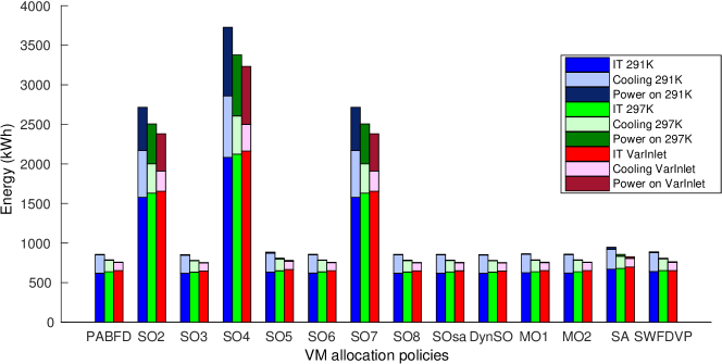
Figure 20: Contributions to data center energy per VM allocation strategy for Workload 3

Figure 21 shows the energy and average SLA percentage comparison for those strategies that outperform the baseline PABFD, which is the baseline that performs better in this scenario, in terms of energy, where SLA is maintained. For this workload, $SO_{SA}$, $SO_{6}$, $SO_{3}$, $MO_{1}$ and DynSO allocation policies offer the best results, in terms of energy savings, when compared to our three baselines. These policies, when combined with VarInlet strategy, provide average savings of 11.78% and 20.19% with respect to SA at 297 K and 291 K respectively, and maximum savings of up to 12.16% and 20.53% respectively for $SO_{3}$. These allocation policies, when compared with $SO_{1}$ also provide average savings of 4.02% and 11.72% at 297 K and 291 K respectively, and maximum savings of up to 4.37% and 12.04% respectively for $SO_{3}$. Finally, comparing the results with the SWFDVP baseline, average savings of 7.22% and 15.51 % and maximum savings of 7.53 % and 15.79% (for $SO_{3}$) are found.

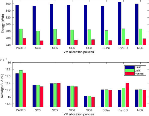
Figure 21: Data center energy and SLA per VM allocation strategy for Workload 3

Tables 5, 6 and  7 provide a summary of the energy savings obtained for the different optimization scenarios for VarInlet cooling strategy, compared with the local baseline PABFD, the global SA baseline and the SWFDVP state-of-the-art baseline policies respectively. The results show that higher energy savings are provided for increasing instantaneous workload variability for both fixed cooling inlet strategies at 291 K and 297 K.

Table 5: Energy savings for VarInlet per VM allocation policy compared with PABFD.

Policy	Energy Savings for VarInlet vs. PABFD (%)
	Workload 1		Workload 2		Workload 3
	297K	291K	297K	291K	297K	291K
$SO_{3}$	6.53	13.60	5.24	13.00	4.37	12.04
$SO_{6}$	6.64	13.71	5.88	13.59	3.80	11.51
$SO_{SA}$	7.07	14.10	5.75	13.47	3.98	11.68
$DynSO$	6.30	13.39	4.83	12.62	4.31	11.98
$MO_{2}$	6.50	13.58	5.04	12.81	3.66	11.39

Table 6: Energy savings for VarInlet per VM allocation policy compared with SA.

Policy	Energy Savings for VarInlet vs. SA (%)
	Workload 1		Workload 2		Workload 3
	297K	291K	297K	291K	297K	291K
$SO_{3}$	13.59	21.28	12.38	19.89	12.16	20.53
$SO_{6}$	13.70	21.38	12.97	20.43	11.63	20.06
$SO_{SA}$	14.09	21.74	12.85	20.33	11.81	20.21
$DynSO$	13.39	21.10	12.00	19.54	12.11	20.48
$MO_{2}$	13.57	21.27	12.19	19.72	11.51	19.94

Table 7: Energy savings for VarInlet per VM allocation policy compared with SWFDVP.

Policy	Energy Savings for VarInlet vs. SWFDVP (%)
	Workload 1		Workload 2		Workload 3
	297K	291K	297K	291K	297K	291K
$SO_{3}$	6.82	14.72	7.09	14.78	7.53	15.79
$SO_{6}$	6.94	14.82	7.72	15.36	7.02	15.33
$SO_{SA}$	7.36	15.21	7.59	15.25	7.18	15.47
$DynSO$	6.60	14.51	6.69	14.41	7.52	15.78
$MO_{2}$	6.80	14.70	6.89	14.60	6.85	15.17

The proposed VM allocation strategies $SO_{3}$, $SO_{6}$, $SO_{SA}$, DynSO, $MO_{2}$ cannot be compared between them in terms of power savings, as their relative savings fall behind the error of our power model. In terms of SLA, the outcomes show that our algorithms maintain the SLA obtained for the baseline policy. The SLA violations are increased by $SO_{6}$ and $SO_{SA}$ for the most variable scenario (Workload 1), and only when compared with the 291 K fixed cooling policy. However, this increment is only of about $0.14\cdot 10^{-4}$. If the SLA is critical for the data center management, $MO_{2}$ provides SLA reductions that are consistent within the 9 scenarios, also offering competitive energy savings. Globally, our $SO_{SA}$ is the strategy that performs better if selected for all the different scenarios with significantly different workload profiles. This approach presents the best savings for Workload 1, which is the more variable one, and a very high savings value for less variable workloads 2 and 3 (for which both baselines are more competitive due to the lower variability). For all the scenarios, the $SO_{SA}$ approach outperforms the PABFD, SA and SWFDVP baselines as can be seen in Table 8. Our local SO based on SA optimization,$SO_{SA}$, leverages the information from a global strategy combined with the information of the overall data center infrastructure provided by our optimization framework.

Table 8: Energy savings for VarInlet in average and for $SO_{SA}$ strategy.

Baseline		Workload 1		Workload 2		Workload 3
		297K	291K	297K	291K	297K	291K
PABFD	average	6.61%	13.67%	5.34%	13.09%	4.02%	11.72%
	$SO_{SA}$	7.07%	14.10%	5.75%	13.47%	3.98%	11.68%
SA	average	13.67%	21.35%	12.48%	19.99%	11.78%	20.19%
	$SO_{SA}$	14.09%	21.74%	12.85%	20.33%	12.16%	20.50%
SWFDVP	average	6.91%	14.79%	7.20%	14.88%	7.22%	15.51%
	$SO_{SA}$	7.36%	15.21%	7.59%	15.25%	7.18%	15.47%

Each workload (1 to 3) is composed of 7 days of real traces obtained each 300 seconds (2016 traces, each of them defining an optimization slot). In terms of computational time the BFD-based approaches show a better performance. The simulation time for the SO policies ($SO_{1}$-$SO_{8}$, DynSO and $SO_{SA}$) ranges from 56 to 84 minutes. $MO_{1}$ and $MO_{2}$ present a simulation time of around 105 minutes. Thus, each minimization (one per optimization slot) for BFD-based approaches takes between 1.66 and 3.12 seconds. On the other hand, the complete simulation of a 7 days-workload takes between 3360 and 5040 minutes to finish for the SA scenario. So, each SA minimization takes between 100 and 150 seconds approximately, and as our SA is configured with 100000 iterations, each iteration takes only 1 millisecond. These results are compliant with the space of solutions explored in each case, numVMs*numHosts=1127*1200 for BFD-based and $numHosts^{numVMs}=1200^{1127}$ for the SA-based approaches. Thus, these results show that the BFD-based algorithms are a lighter implementation in terms of execution time and complexity, but still powerful enough to tackle the joint IT and cooling energy optimization problem like the one described in this research.

Finally, the PUE (Power Usage Effectiveness) is a metric that measures the efficiency of a data center in terms of energy usage. Specifically, it provides information of the amount of energy that is used by the computing equipment in contrast to cooling and other overheads. The PUE value works well with cooling optimizations, as reductions on cooling power result in a higher percentage of the power budget consumed only by IT. On the other hand, for IT optimizations that do not impact on cooling consumption, the PUE does not show the efficiency gained by the IT energy reduction, but reports a negative impact, as it results on a higher percentage of the total power used for cooling purposes. Our research reduces both IT and cooling contributions to final power consumption simultaneously. For fixed cooling baseline policies with set point temperatures of 291 K and 297 K, our infrastructure provides PUE values of 1.37 and 1.23 respectively. Our VarInlet approach, together with our proposed dynamic consolidation $SO_{SA}$, optimizes the PUE in up to 16.05% and 6.5% respectively, providing a PUE value of 1.16, for a dynamic utilization of the IT resources around 80%, that outperforms the state-of-the-art value that is around 1.2.

8 Conclusions

The new optimization framework proposed in this work focuses on considering the energy globally from the data center perspective. In this way, the elements are aware of the evolution of the global energy demand and the thermal behavior of the room. Our decisions are taken based on information from the available subsystems to perform energy optimizations from the technology to the data center level. Metaheuristic algorithms like Simulated Annealing, when used for VM consolidation in data centers, are able to achieve very good results in terms of energy. However, the time that they need to perform the optimizations makes them unsuitable for being used during runtime for this purpose. On the other hand, various local BFD-based policies provide good solutions to the energy problem. They constrain the set of active servers, thus reducing the static energy consumption, but this local strategies do not consider the final status of the data center after each optimization, so the number of VM migrations may be increased. Leveraging the knowledge gathered from both metaheuristic and BFD algorithms helps us to infer models that describe global energy patterns into local strategies, which are faster and lighter to be used for optimizing the energy consumption during runtime under variable conditions. By using this technique we provide the $SO_{SA}$ VM allocation policy that, together with our proposed cooling strategy $VarInlet$, allows us to improve the energy efficiency in scenarios with high workload variability. Our $SO_{SA}$ technique achieved energy savings around 7% and 15%, using two different traditional cooling strategies with fixed set points at 297 K and 291 K respectively, when compared with both local baselines PABFD and SWFDVP. Also, compared with a global SA-based baseline, our local VM allocation policy $SO_{SA}$ provided energy savings of up to 14.09% and 21.74%. For all the scenarios proposed in this research, our optimization algorithms maintain the QoS when compared with a local and a global baseline.

References

- Abbasi et al., 2010 Abbasi, Z., Varsamopoulos, G., and Gupta, S. K. S. (2010). Thermal aware server provisioning and workload distribution for internet data centers. In Proceedings of the 19th ACM International Symposium on High Performance Distributed Computing, HPDC ’10, pages 130–141, New York, NY, USA. ACM.
- Alboaneen et al., 2016 Alboaneen, D. A., Tianfield, H., and Zhang, Y. (2016). Metaheuristic approaches to virtual machine placement in cloud computing: A review. 2016 15th International Symposium on Parallel and Distributed Computing (ISPDC), pages 214–221.
- Arroba et al., 2017 Arroba, P., Moya, J. M., Ayala, J. L., and Buyya, R. (2017). Dynamic voltage and frequency scaling-aware dynamic consolidation of virtual machines for energy efficient cloud data centers. Concurrency and Computation: Practice and Experience, 29(10).
- Arroba et al., 2014 Arroba, P., Risco-Martín, J. L., Zapater, M., Moya, J. M., Ayala, J. L., and Olcoz, K. (2014). Server power modeling for run-time energy optimization of cloud computing facilities. Energy Procedia, 62:401 – 410.
- Ayoub et al., 2012 Ayoub, R., Nath, R., and Rosing, T. (2012). Jetc: Joint energy thermal and cooling management for memory and cpu subsystems in servers. High Performance Computer Architecture (HPCA), 2012 IEEE 18th International Symposium on, pages 1–12.
- Beloglazov and Buyya, 2012 Beloglazov, A. and Buyya, R. (2012). Optimal online deterministic algorithms and adaptive heuristics for energy and performance efficient dynamic consolidation of virtual machines in cloud data centers. Concurrency and Computation: Practice & Experience, 24(13):1397–1420.
- Calheiros et al., 2011 Calheiros, R. N., Ranjan, R., Beloglazov, A., De Rose, C. A. F., and Buyya, R. (2011). Cloudsim: A toolkit for modeling and simulation of cloud computing environments and evaluation of resource provisioning algorithms. Software: Practice and Experience, 41(1):23–50.
- Chan et al., 2012 Chan, C. S., Jin, Y., Wu, Y.-K., Gross, K., Vaidyanathan, K., and Rosing, T. i. (2012). Fan-speed-aware scheduling of data intensive jobs. In Proceedings of the 2012 ACM/IEEE International Symposium on Low Power Electronics and Design, ISLPED ’12, pages 409–414, New York, NY, USA. ACM.
- Chen et al., 2009 Chen, Y., Keys, L., and Katz, R. H. (2009). Towards energy efficient mapreduce. Technical Report UCB/EECS-2009-109, EECS Department, University of California, Berkeley.
- Chowdhury et al., 2015 Chowdhury, M. R., Mahmud, M. R., and Rahman, R. M. (2015). Implementation and performance analysis of various vm placement strategies in cloudsim. Journal of Cloud Computing, 4(1):20.
- Donoghue et al., 2013 Donoghue, A., Inglesant, P., and Lawrence, A. (2013). The EU dreams of renewable-powered datacenters with smart-city addresses. . 451 Research.
- Engbers and Taen, 2014 Engbers, N. and Taen, E. (2014). Green Data Net. Report to IT Room INFRA. European Commision. FP7 ICT 2013.6.2.
- Hamilton, 2009 Hamilton, J. (2009). Cooperative expendable micro-slice servers (cems): Low cost, low power servers for internet-scale services. Proceedings of the 4th Biennial Conf. Innovative Data Systems Research, Asilomar, CA, USA.
- Heilig et al., 2017 Heilig, L., Buyya, R., and Voß, S. (2017). Location-aware brokering for consumers in multi-cloud computing environments. Journal of Network and Computer Applications, 95:79–93.
- Heilig et al., 2016 Heilig, L., Lalla-Ruiz, E., and Voß, S. (2016). A cloud brokerage approach for solving the resource management problem in multi-cloud environments. Computers & Industrial Engineering, 95:16–26.
- Katz, 2009 Katz, R. H. (February 2009). Tech Titans Building Boom. IEEE Spectrum.
- Khelghatdoust et al., 2016 Khelghatdoust, M., Gramoli, V., and Sun, D. (2016). Glap: Distributed dynamic workload consolidation through gossip-based learning. 2016 IEEE International Conference on Cluster Computing (CLUSTER), pages 80–89.
- Kirkpatrick et al., 1983 Kirkpatrick, S., Gelatt, C. D., and Vecchi, M. P. (1983). Optimization by simulated annealing. SCIENCE, 220(4598):671–680.
- Koomey, 2011 Koomey, J. (2011). Growth in data center electricity use 2005 to 2010. Technical report, Report by Analytics Press, completed at the request of The New York Times., Oakland, CA.
- Kumar et al., 2014 Kumar, P., Singh, D., and Kaushik, A. (2014). Power and data aware best fit algorithm for energy saving in cloud computing. International Journal of Computer Science and Information Technologies, 5(5).
- Lewis et al., 2008 Lewis, A., Ghosh, S., and Tzeng, N.-F. (2008). Run-time energy consumption estimation based on workload in server systems. In Proceedings of the 2008 conference on Power aware computing and systems, HotPower’08, pages 4–4, Berkeley, CA, USA. USENIX Association.
- Li et al., 2011 Li, S., Abdelzaher, T., and Yuan, M. (2011). Tapa: Temperature aware power allocation in data center with map-reduce. Green Computing Conference and Workshops (IGCC), 2011 International, pages 1 –8.
- Li et al., 2018 Li, X., Garraghan, P., JIANG, X., Wu, Z., and Xu, J. (2018). Holistic virtual machine scheduling in cloud datacenters towards minimizing total energy. IEEE Transactions on Parallel and Distributed Systems, pages 1–1.
- Markoff and Lohr, 2002 Markoff, J. and Lohr, S. (2002). Intel’s huge bet turns iffy. New York Times Technology Section.
- Melhem et al., 2017 Melhem, S. B., Agarwal, A., Goel, N., and Zaman, M. (2017). Markov prediction model for host load detection and vm placement in live migration. IEEE Access, PP(99):1–1.
- Mitra et al., 2005 Mitra, S., Seifert, N., Zhang, M., Shi, Q., and Kim, K. S. (2005). Robust system design with built-in soft-error resilience. Computer, 38(2):43–52.
- Moore et al., 2005 Moore, J., Chase, J., Ranganathan, P., and Sharma, R. (2005). Making scheduling "cool": temperature-aware workload placement in data centers. In Proceedings of the annual conference on USENIX Annual Technical Conference, ATEC ’05, pages 5–5, Berkeley, CA, USA. USENIX Association.
- Mosa and Paton, 2016 Mosa, A. and Paton, N. W. (2016). Optimizing virtual machine placement for energy and sla in clouds using utility functions. Journal of Cloud Computing, 5(1):17.
- Narendra and Chandrakasan, 2010 Narendra, S. and Chandrakasan, A. (2010). Leakage in Nanometer CMOS Technologies. Integrated Circuits and Systems. Springer.
- Niles, 2010 Niles, S. (2010). Virtualization: Optimized power and cooling to maximize benefits. White paper, APC by Schneider Electric.
- Pires and Barán, 2015 Pires, F. L. and Barán, B. (2015). A virtual machine placement taxonomy. 2015 15th IEEE/ACM International Symposium on Cluster, Cloud and Grid Computing, pages 159–168.
- Ponemon Institute, 2013 Ponemon Institute (2013). 2013 Study on Data Center Outages. Technical report, Ponemon Institute sponsored by Emerson Network Power.
- Primas et al., 2017 Primas, B., Garraghan, P., McKee, D., Summers, J., and Xu, J. (2017). A framework and task allocation analysis for infrastructure independent energy-efficient scheduling in cloud data centers. 2017 IEEE International Conference on Cloud Computing Technology and Science (CloudCom), pages 178–185.
- Quang-Hung et al., 2017 Quang-Hung, N., Son, N. T., and Thoai, N. (2017). Energy-saving virtual machine scheduling in cloud computing with fixed interval constraints. LNCS Transactions on Large-Scale Data- and Knowledge-Centered Systems XXXI - Volume 10140, pages 124–145, New York, NY, USA. Springer-Verlag New York, Inc.
- Quang-Hung and Thoai, 2015 Quang-Hung, N. and Thoai, N. (2015). Energy-efficient vm scheduling in iaas clouds. Future Data and Security Engineering, pages 198–210, Cham. Springer International Publishing.
- Rabaey, 2009 Rabaey, J. (2009). Low Power Design Essentials. Engineering (Springer-11647). Springer.
- Scheihing, 2007 Scheihing, P. (2007). Creating energy efficient data center. Data Center Facilities and Engineering Conference, Washington DC, USA.
- Shen et al., 2015 Shen, S., van Beek, V., and Iosup, A. (2015). Statistical characterization of business-critical workloads hosted in cloud datacenters. 15th IEEE/ACM International Symposium on Cluster, Cloud and Grid Computing, CCGrid’15, Shenzhen, China, 2015, pages 465–474.
- Shrivastava et al., 2017 Shrivastava, A., Patel, V., and Rajak, S. (2017). An energy efficient vm allocation using best fit decreasing minimum migration in cloud environment. International Journal of engineering science and computing, 7(1).
- Solanki and Purohit, 2016 Solanki, N. and Purohit, R. (2016). Energy-aware virtual machine allocations using bin packing algorithms in cloud data centers. International Journal of Engineering and Technical Research, 5.
- Sun et al., 2015 Sun, D., Zhang, G., Yang, S., Zheng, W., Khan, S. U., and Li, K. (2015). Re-stream: Real-time and energy-efficient resource scheduling in big data stream computing environments. Information Sciences, 319:92 – 112. Energy Efficient Data, Services and Memory Management in Big Data Information Systems.
- Usmani and Singh, 2016 Usmani, Z. and Singh, S. (2016). A survey of virtual machine placement techniques in a cloud data center. Procedia Computer Science, 78:491 – 498. 1st International Conference on Information Security & Privacy 2015.
- Wu et al., 2012 Wu, G., Tang, M., Tian, Y.-C., and Li, W. (2012). Energy-efficient virtual machine placement in data centers by genetic algorithm. Proceedings of the 19th International Conference on Neural Information Processing - Volume Part III, pages 315–323, Berlin, Heidelberg. Springer-Verlag.
- Xu and Fortes, 2010 Xu, J. and Fortes, J. A. B. (2010). Multi-objective virtual machine placement in virtualized data center environments. Green Computing and Communications (GreenCom), 2010 IEEE/ACM Int’l Conference on Int’l Conference on Cyber, Physical and Social Computing (CPSCom), pages 179–188.
- Ye et al., 2017 Ye, X., Yin, Y., and Lan, L. (2017). Energy-efficient many-objective virtual machine placement optimization in a cloud computing environment. IEEE Access, 5:16006–16020.