About the magnitude of the $\gamma^{\ast}N\to N(1520)$ transverse amplitudes near $Q^{2}=0$

Abstract

The $\gamma^{\ast}N\to N(1520)$ transition has a property that differs from the other low lying nucleon resonance amplitudes: the magnitude of the transverse helicity amplitudes. The transition helicity amplitudes are defined in terms of square transfer momentum $q^{2}$, or $Q^{2}=-q^{2}$. Near the photon point ($Q^{2}=0$) there is a significant difference in the magnitude of the transverse amplitudes: $A_{3/2}$ is very large and $A_{1/2}$ is very small. This atypical behavior contrasts with the relation between the amplitudes at the pseudothreshold (the limit where the nucleon and the $N(1520)$ are both at rest and $Q^{2}<0$), where $A_{3/2}=A_{1/2}/\sqrt{3}$, and also in the large $Q^{2}$ region, where theory and data suggest that $A_{3/2}$ is suppressed relative to $A_{1/2}$. In the present work, we look for the source of the suppression of the $A_{1/2}$ amplitude at $Q^{2}=0$. The result is easy to understand in first approximation, when we look into the relation between the transverse amplitudes and the elementary form factors, defined by a gauge invariant parametrization of the $\gamma^{\ast}N\to N(1520)$ transition current, near $Q^{2}=0$. There is a partial cancellation between contributions of two elementary form factors near $Q^{2}=0$. We conclude, however, that the correlation between the these elementary form factors at $Q^{2}=0$ is not sufficient to explain the transverse amplitude data below $Q^{2}=1$ GeV². The description the dependence of the transverse amplitudes on $Q^{2}$ requires the determination of the scale of variation of the elementary form factors in the range $Q^{2}=0$…0.5 GeV², a region with almost non existent data. We conclude at the end that the low $Q^{2}$ data for the transverse amplitudes can be well described when we relate the scale of variation of the elementary form factors with the nucleon dipole form factor.

I Introduction

In the last two decades there was a significant progress in the experimental study of the electromagnetic structure of the nucleon ($N$) and the nucleon resonances ($N^{\ast}$). The helicity amplitudes associated with the $\gamma^{\ast}N\to N^{\ast}$ transitions have been measured in detail for the $\Delta(1232)$, $N(1440)$, $N(1520)$ and $N(1535)$ resonances in a range from $Q^{2}=0.25$ GeV² up to 4 or 6 GeV² [1, 3, 2, 4, 5, 6]. The measured helicity amplitudes are: the transverse amplitudes $A_{1/2}$ and $A_{3/2}$ (for spin $J\geq 3/2$) and the longitudinal amplitude $S_{1/2}$. Near the photon point, however, there are still some uncertainties associated with the shape associated with the helicity amplitudes [1, 7, 8]. The selection from the Particle Data Group (PDG) at $Q^{2}=0$ have a large band of variation [9], and for most resonances there are no data below $Q^{2}=0.25$ GeV² [1, 10].

Among the best known experimental resonances the $N(1520)\frac{3}{2}^{-}$ (spin $J=\frac{3}{2}$ and negative parity, $P=-$) has properties that differ from the other low lying nucleon excitations. The transverse amplitudes $A_{1/2}$ and $A_{3/2}$ have completely different magnitudes near the photon point [9], and the helicity amplitudes are related by two conditions near the pseudothreshold point, where $Q^{2}=-(M_{R}-M)^{2}$ [1, 11] ($M$ is the mass of the nucleon and $M_{R}$ is the mass of the nucleon resonance). Most transitions are constrained by only one condition [1, 7, 11]. Although these constraints are valid in a region not directly accessed by electron scattering on nucleons ($Q^{2}<0$), that may not be probed directly in physical experiments, the relations may have a significant impact on the shape of the helicity amplitudes at low $Q^{2}$, when the masses of the nucleon and the nucleon resonance are close [1, 7, 8, 12, 13, 14]. Numerically, the pseudothreshold occurs when $Q^{2}\simeq-0.38$ GeV².

In the present work, we study the magnitude of the $\gamma^{\ast}N\to N(1520)$ transverse amplitudes near $Q^{2}=0$, based on the analytic structure of the transition current and on the correlations between the amplitudes in the low $Q^{2}$ region. We start by reviewing what we know about the transverse amplitudes in three kinematic regions.

Near the pseudothreshold, in addition to the condition associated with Siegert’s theorem [15, 8, 16, 17], one has the relation $A_{3/2}=\sqrt{3}A_{1/2}$ [1, 11, 7]. In the large $Q^{2}$ region, theoretical calculations based on constituent quark counting rules and perturbative QCD arguments indicate that there is a strong dominance of the $A_{1/2}$ amplitude over the $A_{1/2}$ amplitude ($|A_{1/2}|\gg|A_{1/2}|$) [1, 2, 5, 18]. Finally, near $Q^{2}=0$, the can quote the information from the Particle Data Group (PDG) [9]

$$A_{3/2}=+(140\pm 5)\times 10^{-3}\;\mbox{GeV}^{-1/2},$$

$$A_{1/2}=-(22.5\pm 7.5)\times 10^{-3}\;\mbox{GeV}^{-1/2}.$$ (1)

From these results, we can conclude that there is a considerable suppression of $A_{1/2}$ relative to $A_{3/2}$ at the photon point.

We can summarize our knowledge of the ratio $A_{1/2}/A_{3/2}$, in the three regimes, as

$${\cal R}\equiv\frac{A_{1/2}}{A_{3/2}}=\left\{\begin{array}[]{ccc}\frac{1}{\sqrt{3}}&\mbox{if}&Q^{2}=-(M_{R}-M)^{2}\cr\vspace{.1cm}-\epsilon&\mbox{if}&Q^{2}=0\cr\vspace{.1cm}\infty&\mbox{if}&Q^{2}=+\infty\cr\end{array},\right.$$ (5)

where $\epsilon$ represents a small positive value, $\epsilon\simeq 0.18\simeq\frac{1}{5}$, according to the experimental data (1).

At the pseudothreshold, the amplitudes have similar magnitudes (${\cal R}\simeq 0.6$). The suppression of $A_{3/2}$ at large $Q^{2}$ is extensively discussed in the literature [1, 2, 18, 19]. The theoretical challenge is then to understand why is the ratio between the two amplitudes so small in absolute value near $Q^{2}=0$.

From the theoretical point of view, there is some debate about the nature of the $N(1520)$ resonance: if it is dominated by valence quark degrees of freedom, or in alternative, if it is dominated by baryon-meson molecular-like states [1, 19, 6, 20]. The magnitude of $A_{3/2}(0)$ is difficult to explain based solely on the quark core structure of the baryon states. Quark model calculations explain in general only about one third or one half of the measured value of the amplitude [18, 21, 22, 24, 23]. Those estimates are improved when explicit meson cloud dressing or quark-antiquarks excitations are taken into account in quark model calculations [24, 25]. Calculations based on dynamical coupled-channel reaction models, where the baryon resonances are described in terms baryon-meson states [6, 26, 27], predict large contributions to the amplitude $A_{3/2}$ at low $Q^{2}$, in the order of 50% of the experimental values [20]. In the present work, we look for the origin of the difference of magnitudes between $A_{1/2}$ and $A_{3/2}$, based on the numerical contributions for each amplitude, without an explicit reference to the internal degrees of freedom.

The transverse amplitudes can be expressed in terms of the multipole form factors: the magnetic dipole ($G_{M}$) and the electric quadrupole ($G_{E}$) form factors, as defined by Devenish et. al. [1, 2, 11],

$$A_{1/2}=-\frac{1}{4F}T_{1},\hskip 25.6073ptA_{3/2}=-\frac{\sqrt{3}}{4F}T_{2},$$ (6)

where

$$T_{1}\equiv G_{E}-3G_{M},\hskip 25.6073ptT_{2}\equiv G_{E}+G_{M},$$ (7)

and the factor $F$ takes the form

$$F=\frac{1}{e}\frac{2M}{M_{R}-M}\sqrt{\frac{MM_{R}K}{(M_{R}+M)^{2}+Q^{2}}},$$ (8)

with $K=\frac{M_{R}^{2}-M^{2}}{2M_{R}}$, $e=\sqrt{4\pi\alpha}$ and $\alpha\simeq 1/137$ is the hyperfine structure constant.

From the previous relations, we can conclude that $A_{1/2}\simeq 0$, near $Q^{2}=0$ is equivalent to the result $G_{E}\simeq 3G_{M}$. Notice, however, that this analysis only transfers the discussion from helicity amplitudes to the multipole form factors $G_{E}$ and $G_{M}$, and tell us nothing about the correlation between $G_{E}$ and $G_{M}$.

The results $A_{3/2}\simeq 0$ or $G_{E}\simeq 3G_{M}$ can be understood when we write down the relations between the helicity amplitudes and the multipole form factors in terms the elementary form factors, defined by the gauge invariant representation of the transition current for a $J^{P}=\frac{3}{2}^{-}$ nucleon resonance. The transition current can be expressed in terms of 3 independent gauge invariant structures which define 3 independent forms factors that can be labeled as $G_{1}$, $G_{2}$ and $G_{3}$, and are free of kinematic singularities [1, 11]. For convenience, we call these functions elementary form factors.

Using the elementary form factors, we can re-write the transverse amplitudes (6) in the limit $Q^{2}=0$, as

$$A_{1/2} = -\frac{1}{4F_{0}}\,T_{1},$$ (9)

$$A_{3/2} = -\frac{\sqrt{3}}{4F_{0}}\,\left[T_{1}-4\frac{M}{\sqrt{6}}\frac{M_{R}-M}{M_{R}}G_{1}\right],$$ (10)

where $F_{0}={\cal B}\sqrt{M}$ and ${\cal B}=\frac{1}{e}\frac{M}{M_{R}}\sqrt{\frac{M_{R}}{K}}\simeq 3.67$ is dimensionless. The factor $T_{1}$, defined by Eqs. (7), takes the form

$$T_{1}=-4\frac{M}{\sqrt{6}}\left[\frac{M}{M_{R}}G_{1}+\frac{1}{2}(M_{R}+M)G_{2}\right].$$ (11)

From the relations (9)–(11), we can then conclude that in the limit $Q^{2}=0$, the transverse amplitudes depend only on the values of the functions $G_{1}$ and $G_{2}$. We can also conclude that $A_{1/2}\simeq 0$, when $T_{1}$ is negligible, and as a consequence $A_{3/2}\propto\frac{M_{R}-M}{M_{R}}G_{1}$ is large when $G_{1}$ is large. The numerical result for $A_{1/2}$ is then explained when $G_{1}$ and $G_{2}$ are large and have opposite signs. In this case, there is a significant cancellation between the terms in $G_{1}$ and in $G_{2}$. We will conclude, however, that $T_{1}\simeq 0$ ($\epsilon\simeq 0$) provide only a rough explanation of the data. The values of $G_{1}$ and $G_{2}$ at $Q^{2}=0$ have corrections of the order of 30% and 20% respectively when we use the experimental ratio $A_{1/2}/A_{3/2}$ ($\epsilon\simeq 0.2$), instead of $A_{1/2}=0$ ($\epsilon=0$).

At this point, one can ask if the values of $G_{1}(0)$ and $G_{2}(0)$ can help to explain the $Q^{2}$ dependence of $A_{1/2}$ and $A_{3/2}$ in the range $Q^{2}=0$…1 GeV². A simple numerical calculation demonstrates, however, that the shape of the amplitude $A_{3/2}$ cannot be explained without an estimate of the derivative of the elementary form factors $G_{i}$. We conclude at the end that the $A_{1/2}$ and $A_{3/2}$ data can be well described when we consider simple multipole parametrizations of the form factors $G_{i}$, where the scale of variation is determined by the scale of the nucleon dipole form factor, used in parametrizations of the nucleon electromagnetic form factors and some $\gamma^{\ast}N\to N^{\ast}$ transition form factors.

We propose parametrizations of the $A_{1/2}$ and $A_{3/2}$ amplitudes based on our analysis of the amplitudes at $Q^{2}=0$. The parametrizations are consistent with the $Q^{2}=0$…1 GeV² data, within the uncertainties of the available data, and may be tested by future experiments in facilities like MAMI or JLab-12 GeV in the low-$Q^{2}$ region [10]. The precision of the present estimates can be improved once the uncertainties of the $A_{1/2}(0)$ and $A_{3/2}(0)$ data are reduced.

This article is organized as follows: in the next section we present the general formalism for the $\gamma^{\ast}N\to N^{\ast}$ transition form factors and helicity amplitudes for $J^{P}=\frac{3}{2}^{-}$ nucleon resonances, and discuss the relevant limits (pseudothreshold, photon point and large $Q^{2}$). Our numerical analysis of the elementary form factors at the photon point is presented in Sec. III. In Sec. IV, we derive parametrizations of the data based on the our analysis and discuss the limits of the parametrizations. We finalize in Sec. IV with the outlook and conclusions.

II Helicity amplitudes and transition form factors

We discuss now the formalism associated with the $\gamma^{\ast}N\to N(1520)$ transition, and the definition of helicity amplitudes and multipole form factors.

Considering an initial nucleon with the momentum $p$ and a final nucleon resonance with momentum $p^{\prime}$, we can define

$$q=p^{\prime}-p,\hskip 17.07182ptP={\textstyle\frac{1}{2}}(p^{\prime}+p),$$ (12)

as the transfer momentum and the average of the baryons momentum, respectively.

The transition current between a nucleon and a $N^{\ast}$ $J^{P}=\frac{3}{2}^{-}$ state can be written as

$$J^{\mu}=\bar{u}_{\alpha}(p^{\prime})\Gamma^{\alpha\mu}(P,q)\gamma_{5}u(p),$$ (13)

where $u_{\alpha}$, $u$ are the resonance, and the nucleon spinors, respectively, and $\Gamma^{\alpha\mu}$ takes the form [1, 2, 11, 19, 28]

$$\Gamma^{\alpha\mu}(P,q) = \left(q^{\alpha}\gamma^{\mu}-{\not\!q}g^{\alpha\mu}\right)G_{1}+$$ (14)

$$\left[q^{\alpha}P^{\mu}-(P\cdot q)g^{\alpha\mu}\right]G_{2}+$$

$$\left(q^{\alpha}q^{\mu}-q^{2}g^{\alpha\mu}\right)G_{3}.$$

In the previous relation, $G_{i}$ ($i=1,2,3$) are independent functions, free of kinematic singularities, refereed hereafter as elementary form factors. Comparatively with other authors that use the Devenish convention for the operators, and define the second term of Eq. (14) in terms of $p^{\prime}=P+{\textstyle\frac{1}{2}}q$ [1, 2, 11], we follow the Jones and Scadron convention [29] and use $P$ to define the operator associated with $G_{2}$ [29, 19, 28, 12]. The conversion is trivial.

For the representation of the helicity amplitudes, defined at the resonance rest frame, it is convenient to introduce the magnitude of the transfer three-momentum $|{\bf q}|$. This variable can be written in a covariant form as

$$|{\bf q}|=\frac{\sqrt{Q_{+}^{2}Q_{-}^{2}}}{2M_{R}},$$ (15)

using the notation

$$Q_{\pm}^{2}=(M_{R}\pm M)^{2}+Q^{2}.$$ (16)

The magnetic dipole ($G_{M}$) and the electric quadrupole ($G_{E}$) form factors can be calculated inverting the relations (6) and (7)

$$G_{M} = -F\left[{\textstyle\frac{1}{\sqrt{3}}}A_{3/2}-A_{1/2}\right],$$ (17)

$$G_{E} = -F\left[\sqrt{3}A_{3/2}+A_{1/2}\right].$$ (18)

One can also relate the longitudinal (scalar) amplitude $S_{1/2}$ with the Coulomb quadrupole form factor $G_{C}$,

$$S_{1/2}=-\frac{1}{\sqrt{2}F}\frac{|{\bf q}|}{2M_{R}}G_{C}.$$ (19)

Using the expressions (13) and (14), we can write the magnetic dipole and the electric quadrupole form factors in terms of $G_{i}$, as [1, 2]

$$G_{M} = -Z_{R}\,Q_{-}^{2}\frac{G_{1}}{M_{R}},$$ (20)

$$G_{E} = -Z_{R}\left\{[(3M_{R}+M)(M_{R}-M)-Q^{2}]\frac{G_{1}}{M_{R}}\right.$$ (21)

$$\left.\frac{}{}+2(M_{R}^{2}-M^{2})G_{2}-4Q^{2}G_{3}\right\},$$

where $Z_{R}=\frac{1}{\sqrt{6}}\frac{M}{M_{R}-M}$.

Using the previous equations, we conclude that

$$T_{1} = -Z_{R}\left\{4[M(M_{R}-M)-Q^{2}]\frac{G_{1}}{M_{R}}\right.$$ (22)

$$\left.\frac{}{}+2(M_{R}^{2}-M^{2})G_{2}-4Q^{2}G_{3}\right\},$$

$$T_{2} = -Z_{R}\left\{4(M_{R}-M)G_{1}\right.$$ (23)

$$\left.+2(M_{R}^{2}-M^{2})G_{2}-4Q^{2}G_{3}\right\}.$$

We can also write

$$T_{2} = T_{1}-4Z_{R}Q_{-}^{2}\frac{G_{1}}{M_{R}}$$ (24)

$$= T_{1}+4G_{M}.$$

For future discussion, we write down also the relation between the Coulomb quadrupole form factor and the elementary form factors,

$$G_{C} = Z_{R}\left[4M_{R}G_{1}+(3M_{R}^{2}+M^{2}+Q^{2})G_{2}\right.$$ (25)

$$\left.+2(M_{R}^{2}-M^{2}-Q^{2})G_{3}\right].$$

The previous relation can be used to calculate the amplitude $S_{1/2}$, according to Eq. (19). Notice that $S_{1/2}$ and $G_{C}$ cannot be measured at the photon point (because there are no real photons with zero polarization). The relation (25) can be used, however, to estimate $G_{C}$ and $G_{3}$ for values of $Q^{2}$ arbitrarily close to $Q^{2}=0$.

We discuss now briefly the three relevant limits: the pseudothreshold, the photon point and the large $Q^{2}$ limit.

II.1 Pseudothreshold

As mentioned already, when we study the electromagnetic properties based on the helicity amplitudes or the multipole form factors, there are some conditions between those functions that need to be fulfilled when we consider the pseudothreshold limit $Q^{2}=-(M_{R}-M)^{2}$ [1, 11]. These conditions are the consequence of the gauge-invariance structure of the transition current, which requires that the elementary form factors are independent and free of kinematic singularities [11, 29].

There are two conditions to be considered for the $\gamma^{\ast}N\to N\left({\textstyle\frac{3}{2}}^{-}\right)$ multipole transition form factors [11, 12]:

$$G_{M}\propto|{\bf q}|^{2},\hskip 19.91684ptG_{C}=-\frac{M_{R}-M}{M_{R}}G_{E}.$$ (26)

These conditions can be transposed to the helicity amplitudes, as [7, 8]

$$A_{3/2}=\sqrt{3}A_{1/2},$$ (27)

$$(A_{1/2}+\sqrt{3}A_{3/2})=-2\sqrt{2}(M_{R}-M)\frac{S_{1/2}}{|{\bf q}|}.$$ (28)

In addition, it is expected that $S_{1/2}\propto{\cal O}(|{\bf q}|)$ and $A_{1/2}$, $A_{3/2}\propto{\cal O}(1)$, near $|{\bf q}|=0$ [7, 16].

The correlation between the transverse amplitudes (27) is equivalent to the relation $G_{M}=0$ from (26) when $|{\bf q}|=0$.

The second condition for the helicity amplitudes relates the electric amplitude, $E\equiv(A_{3/2}+\sqrt{3}A_{1/2})$, with the scalar amplitude $S_{1/2}$, and correspond to Siegert’s theorem for the $J^{P}=\frac{3}{2}^{-}$ nucleon resonances [1, 32, 30, 31, 16, 17, 8, 14].

Using the relations between the helicity amplitudes and the multipole form factors (20) and (21), and $G_{M}=0$, we can conclude that

$$A_{3/2}=\sqrt{3}A_{1/2}=-\frac{\sqrt{3}}{4F}G_{E},$$ (29)

where $F=\frac{1}{e}\frac{M}{\sqrt{2M_{R}}}\sqrt{\frac{M_{R}+M}{M_{R}-M}}$.

The conditions (26) for the form factors are valid for the nucleon resonances $J^{P}=\frac{3}{2}^{-},\frac{5}{2}^{+},\frac{7}{2}^{-},...$. Modified versions of the conditions for the helicity amplitudes (27) and (28) are also valid for $J^{P}=\frac{5}{2}^{+},\frac{7}{2}^{-},...$ [1]. Among all those nucleon resonances, the $N(1520)\frac{3}{2}^{-}$ resonance is one of the resonances with stronger impact of the pseudothreshold conditions on parametrizations compatible with the available data [7], due to the proximity between pseudothreshold and photon points.

II.2 Photon point

In the limit $Q^{2}=0$, we can write

$$T_{1} = -4\frac{M}{\sqrt{6}}\left\{\frac{M}{M_{R}}G_{1}+\frac{1}{2}(M_{R}+M)G_{2}\right\},$$ (30)

$$T_{2} = -4\frac{M}{\sqrt{6}}\left\{G_{1}+\frac{1}{2}(M_{R}+M)G_{2}\right\}.$$ (31)

We can also write, following Eq. (24)

$$T_{2} = T_{1}-4\frac{M}{\sqrt{6}}(M_{R}-M)\frac{G_{1}}{M_{R}}$$ (32)

$$= T_{1}+4G_{M},$$

and

$$G_{M}=-\frac{M}{\sqrt{6}}(M_{R}-M)\frac{G_{1}}{M_{R}}.$$ (33)

To obtain the previous relations, we used $(M_{R}-M)Z_{R}=\frac{M}{\sqrt{6}}$.

Concerning the scalar amplitude, we can write

$$F_{0}S_{1/2}(0)=-\frac{1}{2\sqrt{3}}\frac{M(M_{R}+M)}{4M_{R}^{2}}$$

$$\times[4M_{R}G_{1}+(3M_{R}^{2}+M^{2})G_{2}+2(M_{R}^{2}-M^{2})G_{3}].$$

II.3 Large $Q^{2}$

The large $Q^{2}$ region has been discussed in detail in the literature [1, 2]. Here, we present the summary. At large $Q^{2}$ the transverse amplitudes follow [1, 33, 34]

$$A_{1/2}\propto\frac{1}{Q^{3}},\hskip 17.07182ptA_{3/2}\propto\frac{1}{Q^{5}},$$ (35)

meaning that $A_{3/2}$ is suppressed relatively to $A_{1/2}$.

The corresponding relations for the form factors are [1, 19]

$$G_{E},\;G_{M}\propto\frac{1}{Q^{4}},$$ (36)

$$G_{E}=-G_{M}+{\cal O}\left(\frac{1}{Q^{6}}\right).$$ (37)

III Form factors $G_{i}$ for $Q^{2}=0$

In the analysis of the transverse amplitudes near $Q^{2}=0$, we consider different approximations. For the discussion, we convert the experimental data (1), into the dimensionless variables

$$\tilde{A}_{3/2}=F_{0}A_{3/2}(0)=+0.498\pm 0.018,$$ (38)

$$\tilde{A}_{1/2}=F_{0}A_{1/2}(0)=-0.080\pm 0.027,$$ (39)

based on the numerical result $F_{0}=3.67\sqrt{M}$.

	$MG_{1}(0)$	$M^{2}G_{2}(0)$	$M^{2}G_{3}(0)$	$A_{3/2}(0)$	$A_{1/2}(0)$	$S_{1/2}(0)$	$G_{M}(0)$	$G_{E}(0)$	Label
$T_{1}=0$	$2.507$	$-1.429$		140	0.0		$-0.287$	$-0.862$
$T_{1}=0.319$	$2.354$	$-1.260$	$\;\;\;0.000$	140	$-22.5$	$-82.7$	$-0.367$	$-0.782$	Multipole 2a
	$2.354$	$-1.260$	$-0.140$	140	$-22.5$	$-73.5$	$-0.367$	$-0.782$	Multipole 2b
	$2.354$	$-1.260$	$-0.278$	140	$-22.5$	$-64.4$	$-0.367$	$-0.782$	Multipole 2c
	$(0.183)$	$(0.134)$

Table 1: Model parameters $G_{1}(0)$, $G_{2}(0)$, according with the values for the amplitudes $A_{3/2}(0)$, $A_{1/2}(0)$. We include also the limit of $S_{1/2}(Q^{2})$ for $Q^{2}=0$, based on the values of $G_{3}(0)$. The amplitudes are in units $10^{-3}$ GeV^-1/2. In the last row, the values between commas are the uncertainties of $MG_{1}(0)$ and $M^{2}G_{2}(0)$, based on the data for the transverse amplitudes. The model with $T_{1}\neq 0$ has $T_{2}=-1.149$.

Notice that, since the comparison between amplitudes is made in units $10^{-3}$ GeV^-1/2, the first quantity ($\simeq 500\times 10^{-3}$) can be regarded as a large number, and the second quantity ($\simeq-80\times 10^{-3}$) can be regarded as a small number.

We can use the results (38) and (39), to calculate the corresponding form factors $G_{1}$ and $G_{2}$ for $Q^{2}=0$. Inverting the relations (9)–(11), one obtains

$$MG_{1}={\cal R}\left(\frac{1}{\sqrt{3}}\tilde{A}_{3/2}-\tilde{A}_{1/2}\right),$$ (40)

$$M^{2}G_{2}=-\frac{2M}{M_{R}+M}\frac{M}{M_{R}}{\cal R}\left(\frac{1}{\sqrt{3}}\tilde{A}_{3/2}-\frac{M_{R}}{M}\tilde{A}_{1/2}\right),$$

(41)

where ${\cal R}=\frac{\sqrt{6}M_{R}}{M_{R}-M}$. The factors $M$ and $M^{2}$ are included to generate dimensionless expressions.

In the introduction, we discussed the approximation $\tilde{A}_{1/2}=0$ ($T_{1}=0$), based on Eqs. (9) and (10). In that case, we obtain $G_{2}=-\frac{2}{M_{R}+M}\frac{M}{M_{R}}G_{1}$. Now, we can notice, using the relations (40) and (41), that the condition $T_{1}=0$ provide only a rough approximation, since $\tilde{A}_{1/2}$ is combined in fact with $\tilde{A}_{3/2}/\sqrt{3}$. Neglecting $\tilde{A}_{1/2}$ in the estimates of $G_{1}$ and $G_{2}$ has an impact of 28% for $G_{1}$ and of 17% for $G_{2}$.

The relations (40) and (41) can also used to explain the significant cancellation in $T_{1}$. The effect can be observed when we write $T_{1}$ on the form $T_{1}=-4\frac{M}{\sqrt{6}}t_{1}$, where

$$t_{1}=\frac{M}{M_{R}}G_{1}+\frac{1}{2}(M_{R}+M)G_{2}.$$ (42)

For that purpose, we write the two terms as

$$\frac{M}{M_{R}}G_{1} = \frac{{\cal R}}{M_{R}}\left(\frac{1}{\sqrt{3}}\tilde{A}_{3/2}-\tilde{A}_{1/2}\right),$$

$$\frac{1}{2}(M_{R}+M)G_{2} = -\frac{{\cal R}}{M_{R}}\left(\frac{1}{\sqrt{3}}\tilde{A}_{3/2}-\tilde{A}_{1/2}\right)$$

$$+\frac{{\cal R}}{M_{R}}\frac{M_{R}-M}{M}\tilde{A}_{1/2}.$$

In this form, one concludes that the first term of $\frac{1}{2}(M_{R}+M)G_{2}$ cancels the term in $G_{1}$, and only the term proportional to $\tilde{A}_{1/2}$ survives the sum. The correction term is 13% of the term in $G_{1}$. In units $10^{-3}$ the term in $G_{1}$ and the term in $G_{2}$ are large numbers with opposite signs.

The dominance of the amplitude $A_{3/2}$ is still explained by the small magnitude of $T_{1}$. When we can neglect $T_{1}$ in Eq. (32), we conclude that $T_{2}\propto G_{1}$. Thus, the amplitude $A_{3/2}$ is large when $T_{2}$ is large, and $T_{1}$ is small in comparison with $T_{2}$. However, when we look for (31): $T_{2}=-4\frac{M}{\sqrt{6}}t_{2}$, with $t_{2}=G_{1}+\frac{1}{2}(M_{R}+M)G_{2}$, we conclude that $T_{2}$ is large because there is only a partial cancellation between the two large terms.

To summarize, the combination of the results for the transverse amplitudes is a consequence of the large magnitude of the form factors $G_{1}$ and $-G_{2}$. In $A_{1/2}$, one has a significant cancellation between the term in $G_{1}$ and the term in $G_{2}$. In $A_{3/2}$, the term in $G_{1}$ is enhanced and the suppression between the terms is attenuated. We conclude also that in first approximation (leading order in $\tilde{A}_{1/2}$), one has $A_{3/2}\propto G_{1}$.

The values of $G_{1}$ and $G_{2}$ for $Q^{2}=0$ are presented in Table 1 for the cases $T_{1}=0$ and $T_{1}\neq 0$. The first row ($T_{1}=0$) gives the results when we use $A_{1/2}(0)=0$, and the second row gives the result when $T_{1}\neq 0$ is fixed by the experimental value of $A_{1/2}(0)$. In the second row, we include also $G_{3}(0)=0$. The last four rows and the effect of $G_{3}(0)$ are discussed in the next sections.

The comparison between the first two rows demonstrate how important is the inclusion of the experimental value of $A_{1/2}(0)$, instead of $A_{1/2}(0)=0$, in the determination of the first two elementary form factors. The effect can also be seen in the results for $G_{M}(0)$ and $G_{E}(0)$. The differences are about 20% for the magnetic form factor and 10% for the electric form factor.

In the next sections, we use the estimated values for $G_{1}$ and $G_{2}$ at $Q^{2}=0$ to test if we can derive parametrizations that may explain the experimental data for the amplitudes $A_{1/2}$ and $A_{3/2}$, up to a certain range of $Q^{2}$. Due to the approximated character of the parametrizations, we restrict the analysis to the region $Q^{2}<1$ GeV². To estimate the uncertainties of the parametrizations, we calculate also the uncertainties of $G_{1}$ and $G_{2}$ at $Q^{2}=0$, based on the relations (40) and (41) and the data (1), with the errors combined in quadrature. The numerical values for the uncertainties of $G_{1}(0)$ and $G_{2}(0)$ are included in the last row of Table 1 (between brackets). The relative errors are 7.8% for $G_{1}$ and 10.6% for $G_{2}$.

IV Form factors $G_{i}$ for $Q^{2}>0$

In this section, we discuss possible parametrizations of the amplitudes $A_{1/2}$ and $A_{3/2}$ for $Q^{2}\leq 1$ GeV² based on the values of $G_{1}(0)$ and $G_{2}(0)$ calculated in the previous section.

In the following, we consider the $\gamma^{\ast}N\to N(1520)$ helicity amplitude data from experiments at CLAS/JLab on single pion electroproduction [35] and on charged double pion electroproduction [36, 20], and the PDG selection for $Q^{2}=0$ [9]. These CLAS/JLab experiments determine the all set of helicity amplitudes ($A_{1/2}$, $A_{3/2}$ and $S_{1/2}$). The $\pi N$ ($\sim 60\%$) and the $\pi\pi N$ ($\sim 30\%$) channels are the dominant $N(1520)$ decay channels [9]. There are additional data associated with different experiments for the transverse amplitudes [37], but the data analysis is based on the assumption that $S_{1/2}\equiv 0$, an approximation that is not valid at low $Q^{2}$ [35].

In a first stage, we ignore the role of the form factor $G_{3}$, setting $G_{3}\equiv 0$, since no information about $G_{3}$ can be obtained from the transverse amplitudes at $Q^{2}=0$. We notice, however, that $G_{3}$ contributes to the amplitudes $A_{1/2}$ and $A_{3/2}$ for $Q^{2}\neq 0$, since $T_{1}$ and $T_{2}$ include the term $4Z_{R}Q^{2}G_{3}$ [see Eqs.(22) and (23)]. Later on, we estimate the impact of nonzero values for $G_{3}(0)$.

From the previous section, we concluded already that $A_{1/2}(0)\simeq 0$ is not a very good approximation. In the following, we consider then parametrizations based on the Eqs. (40) and (41) consistent with the experimental value of $A_{1/2}(0)$. The numerical values are included in the lower part of Table 1 (with $T_{1}=0.319$).

We divided our analysis in several steps.

IV.1 Parametrization with constant form factors $G_{i}$

The simplest parametrization can be obtained assuming that the form factors $G_{1}(Q^{2})$ and $G_{2}(Q^{2})$ do not vary significantly in the region $Q^{2}=0$…1 GeV² (meaning that in that range the derivatives of those form factors are zero or negligible). We label this approximation as the constant form factor parametrization. The values of $G_{i}(0)$ are the ones presented on Table 1 in the first row with $T_{1}=0.319$. As mentioned already, we assume for now that $G_{3}(0)=0$.

      

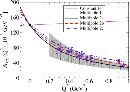
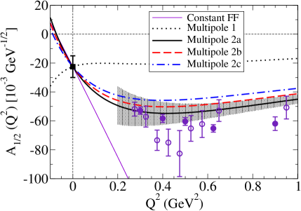
Figure 1: Transverse amplitudes $A_{1/2}$ and $A_{3/2}$ in terms of $Q^{2}$. The data are from JLab/CLAS one pion production (solid bullets) [35], JLab/CLAS two pion production (empty bullets) [36, 20] and PDG (square) [9]. The labels correspond to the parameters from Table 1.

      

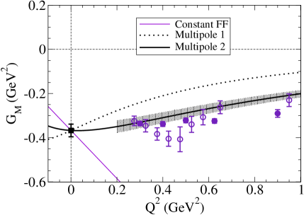
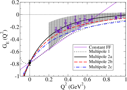
Figure 2: Multipole form factors $G_{E}$ and $G_{M}$ in terms of $Q^{2}$. Data description as in Fig. 1. The labels correspond to the parameters from Table 1.

The constant form factor estimates are presented in Fig. 1 for the amplitudes and in Fig. 2 for the multipole form factors. Notice in the figures the lack of data for the interval $Q^{2}=0$…0.28 GeV². This omission difficult the determination of the shape of the helicity amplitudes near the photon point [1, 7].

In Figs. 1 and 2, we distinguish between the CLAS data from one pion production [35] from double pion production [36, 20]. Some differences between the two sets can be observed for the function $A_{3/2}$ and $G_{M}$ in the range $Q^{2}=0.35$…0.50 GeV². The data are, however, compatible within the two standard deviation range. More accurate data in that range may help to determine the shape of the transverse amplitudes at low $Q^{2}$.

We present the calculations the range $Q^{2}=-0.1$…1 GeV² for a better visualization of the results near $Q^{2}=0$. The lower limit of the graph in $Q^{2}$ can be extended down to the pseudothreshold $Q^{2}\simeq-0.4$ GeV², in order to visualize the consequences of the pseudothreshold constraints. We notice, however, that the pseudothreshold conditions are automatically satisfied by the use of elementary form factors $G_{i}$ when they have no singularities in the range $Q^{2}>-(M_{R}-M)^{2}$. At the end, we discuss the properties of $G_{M}$ near the pseudothreshold.

Before discussing the amplitudes $A_{1/2}$ and $A_{3/2}$ it is important to discuss the properties of the form factors $G_{E}$ and $G_{M}$ when the form factors $G_{i}$ are constants. From the relations (20) and (21), we can conclude that the multipole form factors ($G_{E}$ and $G_{M}$) are linear functions of $Q^{2}$.

As for the transverse amplitudes, we can notice that they are written in the form $A_{1/2}\propto\sqrt{1+\tau}\;T_{1}$ and $A_{3/2}\propto\sqrt{1+\tau}\;T_{2}$, where $T_{1}$ and $T_{2}$ are linear functions and $\tau=Q^{2}/(M_{R}+M)^{2}$ [See Eqs. (6)–(8)]. Since in the region of study $\tau\ll 1$ (because $Q^{2}\ll 6.05$ GeV²), one can write $\sqrt{1+\tau}\simeq 1+\frac{1}{2}\frac{Q^{2}}{(M_{R}+M)^{2}}$, and conclude that in the region $Q^{2}\leq 1$ GeV², the amplitudes are well approximated by linear functions.

We can now discuss the numerical results for the amplitudes $A_{1/2}$ and $A_{3/2}$ within the constant form factor approximation. The estimates are presented in Fig. 1 by the thin solid line (labeled as Constant FF). The model estimate $A_{3/2}\simeq 140$ $\times 10^{-3}$ GeV^-1/2, contrasts with the sharp suppression of the experimental amplitude, when $Q^{2}$ increases. The estimate of $A_{3/2}$ manifests only a weak dependence on $Q^{2}$, because $A_{3/2}\propto\sqrt{1+\tau}\;T_{2}$ and $T_{2}$ is a constant. The conclusion is then that the amplitude $A_{3/2}$ follow $A_{3/2}\propto 1+\frac{1}{2}\frac{Q^{2}}{(M_{R}+M)^{2}}$, in the range of study, an almost constant function. As for the amplitude $A_{1/2}$, we observe also an almost linear function of $Q^{2}$, in flagrant disagreement with the data. The conclusion is then, that the constant form factor approximation for the functions $G_{i}$ fails completely the description of the amplitudes $A_{1/2}$ and $A_{3/2}$.

The corresponding results for $G_{E}$ and $G_{M}$ are presented in Fig. 2. In this case, one obtains linear functions, that fail in general the description of the data.

The corollary of this first analysis is that, the description of the transverse amplitudes requires in addition to the values of the functions $G_{1}$ and $G_{2}$ at $Q^{2}=0$, the determination of the scale of variation of those functions. In simple terms, we need an estimate of the derivatives of the form factors $G_{1}$, $G_{2}$ and eventually $G_{3}$, if we want to describe the data in the range $Q^{2}=0$…1 GeV².

IV.2 Parametrization of $G_{i}$ by multipole functions – universal cutoff

Once concluded that the data are not consistent with parametrizations based on constant elementary form factors, we look for parametrizations based on multipole functions. These kind of parametrizations is considered, for instance in the study of the nucleon electromagnetic form factors, where the main dependence is regulated by a simple dipole function. Based on the expected asymptotic dependence of the functions $G_{i}$ in the large $Q^{2}$ region, we consider the multipole parametrizations

$$G_{1}(Q^{2})=\frac{G_{1}(0)}{\left(1+\frac{Q^{2}}{\Lambda_{3}^{2}}\right)^{3}},\hskip 17.07182ptG_{2,3}(Q^{2})=\frac{G_{2,3}(0)}{\left(1+\frac{Q^{2}}{\Lambda_{4}^{2}}\right)^{4}},$$

(43)

where we labeled the square form factor cutoffs $\Lambda_{n}^{2}$ by the power $n$ of the multipole. We assume then that $G_{2}$ and $G_{3}$ (when $G_{3}(0)\neq 0$) are regulated by the same cutoff. The powers of Eq. (43) are the ones compatible with the expected falloffs for the helicity amplitudes (35) and the multipole form factors (36) and (37).

The multipole functions take into account implicitly, the leading order dependence of the form factors $G_{i}$ on $Q^{2}$. The method had been used in chiral effective field theory to include next-leading order contributions and improve the convergence of the calculations [38]. It is also known that simple smooth parametrizations of $\gamma^{\ast}N\to N^{\ast}$ data are obtained for most low lying nucleon resonances when the functions are normalized by an appropriated multipole [39].

One of the simplest parametrizations is obtained when we assume that the scale of variation of the form factors $G_{i}$ (associated with the square cutoffs $\Lambda_{3}^{2}$ and $\Lambda_{4}^{2}$) can be the same for all the form factors ($\Lambda_{3}^{2}=\Lambda_{4}^{2}$). The condition $\Lambda_{3}^{2}=\Lambda_{4}^{2}$ defines the universal cutoff approximation.

Inspired by the nucleon dipole function

$$G_{D}(Q^{2})=\frac{1}{\left(1+\frac{Q^{2}}{\Lambda_{D}^{2}}\right)^{2}},$$ (44)

where $\Lambda_{D}^{2}=0.71$ GeV², we consider a parametrization where

$$\Lambda_{3}^{2}=\Lambda_{4}^{2}=\Lambda_{D}^{2}.$$ (45)

The results of the universal form factor parametrization are represented in Figs. 1 and 2 by the dotted line and are labeled as Multipole 1. We can notice in the figure for the amplitudes (Fig. 1), the failure in the description of the amplitude $A_{1/2}$. Also worth noticing is the shape the amplitude $A_{3/2}$ near $Q^{2}=0$. Although no data exists below $Q^{2}=0.28$ GeV², theoretical models predict in general a sharp and fast falloff of the amplitude near $Q^{2}=0$. In contrast, the line Multipole 1 has an almost zero derivative at $Q^{2}=0$.

In the constant cutoff approximation, we can also treat the cutoff $\Lambda_{3}=\Lambda_{4}$ as an adjustable parameter, different from $\Lambda_{D}$, to be determined by a fit to the data. Different values of the cutoffs lead, however, to similar results. The combination of the form factors $G_{1}$ and $G_{2}$ on $T_{1}$ and $T_{2}$ are such that generate almost an almost constant estimate for $A_{1/2}$, and an almost zero derivative to $A_{3/2}$ near $Q^{2}=0$.

The conclusion of this section is then that the data are not consistent with multipole parametrizations based on the same cutoff for $G_{1}$ and $G_{2}$.

IV.3 Parametrization of $G_{i}$ by multipole functions – natural scale

Since the universal cutoff fails to provide a description of the low $Q^{2}$ transverse amplitude data, we look for alternative ways of defining the scale of variation of the elementary form factors $G_{i}$. Recalling that the nucleon elastic form factors and some inelastic transitions, such as the $\gamma^{\ast}N\to\Delta(1232)$ magnetic form factor, scale at sufficient small $Q^{2}$ with the dipole function (44), we wondered if the same scale can be used for the functions $G_{i}$. Since the functions are defined by different powers for the multipoles, the similarity of the functions $G_{i}$ with $G_{D}$ must be imposed for low $Q^{2}$. We consider then the conditions near $Q^{2}=0$,

$$\left(1+\frac{Q^{2}}{\Lambda_{3}^{2}}\right)^{-3} \simeq \left(1+\frac{Q^{2}}{\Lambda_{D}^{2}}\right)^{-2},$$ (46)

$$\left(1+\frac{Q^{2}}{\Lambda_{4}^{2}}\right)^{-4} \simeq \left(1+\frac{Q^{2}}{\Lambda_{D}^{2}}\right)^{-2},$$ (47)

The equivalence of the previous expansions near $Q^{2}=0$ implies that

$$\Lambda_{3}^{2}=\frac{3}{2}\Lambda_{D}^{2},\hskip 17.07182pt\Lambda_{4}^{2}=2\Lambda_{D}^{2}.$$ (48)

Numerically, one has $\Lambda_{3}^{2}\simeq 1.07$ GeV² and $\Lambda_{4}^{2}\simeq 1.42$ GeV².

The numerical results associated to the multipole parametrization (43) with the cutoffs (48) and $G_{3}(0)=0$ are presented in Figs. 1 and 2 by the thick solid line, and are labeled as Multipole 2a. Notice the closeness between the lines and the data.

Concerning the results from Fig. 2 for $G_{M}$, a note is in order. Since $G_{M}$ depend only on $G_{1}$, all estimates discussed in this section have the same result for $G_{M}$ (thick solid line). In the figure, we use the label Multipole 2.

The results of the parametrization Multipole 2a demonstrate that a reliable description of the $\gamma^{\ast}N\to N(1520)$ transverse amplitude data can be achieved when we assume the natural scale for the elementary form factors $G_{i}$.

We can now discuss the effect of the form factor $G_{3}$ in parametrizations of the data based on multipole functions. Although $G_{3}(0)$ cannot be determined by the $A_{1/2}(0)$ and $A_{3/2}(0)$ data, indirect information can be obtained from the amplitude $S_{1/2}$ at low $Q^{2}$. Unfortunately, no data below $Q^{2}=0.28$ GeV² are available to make a reliable estimate of $S_{1/2}(0)$, and consequently an estimate of $G_{3}(0)$.

In these conditions, one has to rely on theoretical extrapolations of the data. We consider then a parametrization of the data from Ref. [7], compatible with the pseudothreshold constraints of the helicity amplitudes, and also with the low $Q^{2}$ data for $A_{1/2}$ and $A_{3/2}$. The value of $S_{1/2}(0)$ determined by that parametrization is $S_{1/2}(0)=-64.4\times 10^{-3}$ GeV^-1/2. Combining this result with the present estimates of $G_{1}(0)$ and $G_{2}(0)$, one obtains $M^{2}G_{3}(0)=-0.278$.

In addition to the parametrization discussed earlier (Multipole 2a, $G_{3}(0)=0$), we consider also a parametrization with an intermediate value for $G_{3}(0)$, fixed by $M^{2}G_{3}(0)=-0.14$, labeled as Multipole 2b, and a parametrization associated with value of $S_{1/2}(0)$ mentioned above (Multipole 2c). All parameters and associated values for $S_{1/2}(0)$ are presented in the last four rows of Table 1.

The parametrizations labeled as Multipole 2b and Multipole 2c are also represented in Figs. 1 and 2 by the dashed lines (Multipole 2b) and the dashed-dotted lines (Multipole 2c).

Since these parametrizations (Multipole 2a, 2b, 2c) are defined by the values of $G_{1}(0)$ and $G_{2}(0)$ determined by the transverse amplitudes at $Q^{2}=0$, one can also calculate the band of variation of the parametrizations based on the uncertainties of the parameters. For clarity, we include only the band of variation associated with the Multipole 2a. The others have similar ranges of variation from the central lines. The bands of variation are large for estimates near $Q^{2}=0$, when the errors are added in quadrature, mainly due to the large relative uncertainty of $A_{1/2}(0)$. For that reason, we restrict the representation to $Q^{2}\geq 0.2$ GeV². The width of the bands decreases when $Q^{2}$ increases due to the reduction of the values of the functions $G_{i}$. More accurate experimental estimates of $A_{1/2}(0)$ and $A_{3/2}(0)$ will narrow the uncertainties of the estimates based on Eqs. (40), (41), (43) and (48).

From the analysis of the amplitudes (Fig. 1), we can conclude that the best description of the amplitude $A_{1/2}$ is obtained with Multipole 2a ($G_{3}=0$). Notice, however, that Multipole 2b provide also a fair description of the data when the uncertainties are taken into account. As for the amplitude $A_{3/2}$, the Multipole 2b gives the best description when we consider the central values, but Multipole 2a and Multipole 2c are also consistent with the data, when we take into account the uncertainties (upper error band for Multipole 2a and lower error band for Multipole 2c). Overall Multipole 2a and Multipole 2b give the best combined description of the transverse amplitudes within the uncertainty bands. The agreement with the data is better for $Q^{2}\leq 0.7$ GeV².

The preference for the parametrizations Multipole 2a and Multipole 2b, favors also models with large magnitudes for the absolute values of the scalar amplitude $S_{1/2}(0)$, associated with the range $-$(75…85)$\times 10^{-3}$ GeV^-1/2, as indicated in Table 1.

Similar conclusions are obtained when we look for the multipole form factors $G_{E}$ and $G_{M}$ (Fig. 2). All parametrizations are equivalent for $G_{M}$. The data for $G_{E}$ favors the parametrizations Multipole 2a and Multipole 2b, within the intervals of variation.

In the graph for $G_{M}$, one can also observe that the function is very smooth near $Q^{2}=0$, contrasting with the sharp variation of $G_{E}$. This effect is a consequence of the particular condition for $G_{M}$ at the pseudothreshold, as discussed in Sec. II.1. No equivalent condition exist for $G_{E}$ and $G_{C}$ (related by $G_{E}\propto G_{C}$). Both functions, $G_{E}$ and $G_{C}$, are finite at the pseudothreshold.

A consequence of the condition $G_{M}=0$ at the pseudothreshold is that we can expect a turning point of the function below $Q^{2}=0.2$ GeV². The present calculations suggest that the turning point is close to $Q^{2}=0$, meaning that the derivative of $G_{M}$ at photon point is close to zero. Considering the relation between $G_{M}$ and $G_{1}$, we can conclude that $(M_{R}-M)^{2}\frac{dG_{M}}{dQ^{2}}(0)=\left(1-3\frac{(M_{R}-M)^{2}}{\Lambda_{3}^{2}}\right)G_{M}(0)\simeq 0.05G_{M}(0)$, consistent with a very small value for $\frac{dG_{M}}{dQ^{2}}(0)$. This result is a direct consequence of the parameter $\Lambda_{3}^{2}=1.07$ GeV².

IV.4 Discussion

The parametrizations discussed above are based on two parameters, $G_{1}(0)$ and $G_{2}(0)$, a cutoff determined by theoretical arguments, and some tentative estimates of $G_{3}(0)$. Two of the parametrizations provide good descriptions of the data for $A_{1/2}$ and $A_{3/2}$ for $Q^{2}<1$ GeV², and determine also the possible range variation for the amplitude $S_{1/2}$ near $Q^{2}=0$.

From our analysis, we conclude also that the data favor parametrizations with multipole functions regulated by large cutoffs ($\Lambda_{3}^{2}$, $\Lambda_{4}^{2}>1$ GeV²) and slower falloffs. The considered cutoffs are larger than the cutoff associated with the nucleon elastic form factors ($\Lambda_{D}^{2}\simeq 0.7$ GeV²).

In principle, more accurate estimates can be obtained considering extensions of the multipole parametrizations, where the second derivatives of $G_{i}$ are adjusted by the low $Q^{2}$ data. We did not test this possibility, because the main goal of the present work is the understanding of the $Q^{2}=0$ and low $Q^{2}$ data based on a minimal number of parameters and assumptions.

The parametrizations proposed here may be tested in a near future by experiments in the range $Q^{2}=0$…0.3 GeV², in order to fill the gap in the experimental studies of the $N(1520)$ resonance. That data may be acquired at MAMI ($Q^{2}>0.2$ GeV²) and JLab ($Q^{2}>0.05$ GeV²) [10, 4].

New data can help to determine the shape of the transverse amplitudes below $Q^{2}=0.3$ GeV², and impose more accurate constraints on parametrizations of the data near $Q^{2}=0$ [7]. The knowledge of the $Q^{2}$ dependence of the helicity amplitudes near $Q^{2}=0$ is important for the study of the $\gamma^{\ast}N\to N(1520)$ in the timelike region ($Q^{2}<0$), including the Dalitz decay of the $N(1520)$ state ($N(1520)\to e^{+}e^{-}N$) [19, 40].

V Outlook and conclusions

The $N(1520)$ resonance is among the nucleon excitations that are better known experimentally. It differs from the other low lying nucleon resonances by its properties. The transverse amplitudes $A_{1/2}$ and $A_{3/2}$ have completely different magnitudes at $Q^{2}=0$, and are subject to relevant constraints at low $Q^{2}$, due to the proximity between the pseudothreshold $Q^{2}=-(M_{R}-M)^{2}$ and the photon point.

In the present work, we look for the origin of the difference of magnitudes between the transverse amplitudes at very low $Q^{2}$. We concluded that the result is related to a significant cancellation near $Q^{2}=0$ of the contributions associated with two elementary form factors ($G_{1}$ and $G_{2}$), defined by a gauge-invariant parametrization of the transition current. We concluded also that, the correlation between the elementary form factors does not hold for larger values of $Q^{2}$.

To explain the shape of the amplitudes $A_{1/2}$ and $A_{3/2}$ below $Q^{2}=1$ GeV², in addition to the values of $G_{1}$ and $G_{2}$ at $Q^{2}=0$, one needs to know the scale of variation of the elementary form factors $G_{1}$, $G_{2}$ and $G_{3}$. We obtain a fair description of the $Q^{2}\leq 0.7$ GeV² data when the scale of variation of the elementary form factors is correlated to the natural scale of the $\gamma^{\ast}N\to N^{\ast}$ transition amplitudes, defined by the nucleon dipole form factor.

Different parametrizations can be derived depending on the projected value of the scalar amplitude $S_{1/2}$ near $Q^{2}=0$. Those parametrizations are compatible with the experimental data for the transverse amplitudes within the uncertainties of the data for $Q^{2}=0$. The uncertainties can be reduced once the more accurate determinations of the transverse amplitudes are provided, mainly for $A_{1/2}(0)$. The proposed parametrizations explain also the smooth behavior of the magnetic dipole form factor $G_{M}$ near $Q^{2}=0$, suggested by the data.

Our analysis of the transverse amplitudes $A_{1/2}$ and $A_{3/2}$ for finite $Q^{2}$ allows us to make an estimate of the range of variation of the scalar amplitude $S_{1/2}$ near $Q^{2}=0$, in a region for which there are not data available. Our parametrizations are compatible with values of $S_{1/2}(Q^{2})$ in the range from $-85\times 10^{-3}$ GeV^-1/2 to $-75\times 10^{-3}$ GeV^-1/2, for values of $Q^{2}$ near the photon point. The parametrizations discussed in the present work may be tested in future measurements of the transverse and longitudinal amplitudes for $0<Q^{2}<0.28$ GeV².

- [1] G. Ramalho and M. T. Peña, [arXiv:2306.13900 [hep-ph]].
- [2] I. G. Aznauryan and V. D. Burkert, Prog. Part. Nucl. Phys. 67, 1 (2012) [arXiv:1109.1720 [hep-ph]].
- [3] I. G. Aznauryan et al., Int. J. Mod. Phys. E 22, 1330015 (2013) [arXiv:1212.4891 [nucl-th]].
- [4] V. I. Mokeev, P. Achenbach, V. D. Burkert, D. S. Carman, R. W. Gothe, A. N. Hiller Blin, E. L. Isupov, K. Joo, K. Neupane and A. Trivedi, Phys. Rev. C 108, 025204 (2023) [arXiv:2306.13777 [nucl-ex]].
- [5] D. Drechsel, S. S. Kamalov and L. Tiator, Eur. Phys. J. A 34, 69 (2007) [arXiv:0710.0306 [nucl-th]].
- [6] V. D. Burkert and T. S. H. Lee, Int. J. Mod. Phys. E 13, 1035 (2004) [nucl-ex/0407020].
- [7] G. Ramalho, Phys. Rev. D 100, 114014 (2019) [arXiv:1909.00013 [hep-ph]].
- [8] L. Tiator, Few Body Syst. 57, 1087-1093 (2016).
- [9] R. L. Workman et al. [Particle Data Group], PTEP 2022, 083C01 (2022).
- [10] V. I. Mokeev et al. [CLAS], Few Body Syst. 63, 59 (2022) [arXiv:2202.04180 [nucl-ex]].
- [11] R. C. E. Devenish, T. S. Eisenschitz and J. G. Korner, Phys. Rev. D 14, 3063 (1976).
- [12] G. Ramalho, Phys. Rev. D 93, 113012 (2016) [arXiv:1602.03832 [hep-ph]].
- [13] G. Ramalho, Phys. Rev. D 94, 114001 (2016) [arXiv:1606.03042 [hep-ph]].
- [14] G. Ramalho, Phys. Lett. B 759, 126 (2016) [arXiv:1602.03444 [hep-ph]].
- [15] Siegert’s theorem is a general condition valid for the transitions that relate the electric amplitude (combination of and ) and the scalar/longitudinal amplitude near .
- [16] D. Drechsel and L. Tiator, J. Phys. G 18, 449-497 (1992).
- [17] A. J. Buchmann, E. Hernandez, U. Meyer and A. Faessler Phys. Rev. C 58, 2478 (1998).
- [18] M. Warns, W. Pfeil and H. Rollnik, Phys. Rev. D 42, 2215 (1990).
- [19] G. Ramalho and M. T. Peña, Phys. Rev. D 89, 094016 (2014) [arXiv:1309.0730 [hep-ph]]; G. Ramalho and M. T. Peña, Phys. Rev. D 95, 014003 (2017) [arXiv:1610.08788 [nucl-th]].
- [20] V. I. Mokeev, V. D. Burkert, D. S. Carman, L. Elouadrhiri, G. V. Fedotov, E. N. Golovatch, R. W. Gothe, K. Hicks, B. S. Ishkhanov and E. L. Isupov, et al. Phys. Rev. C 93, 025206 (2016) [arXiv:1509.05460 [nucl-ex]].
- [21] D. Merten, R. Ricken, M. Koll, B. Metsch and H. Petry, Eur. Phys. J. A 13, 477 (2002) [arXiv:hep-ph/0104029 [hep-ph]].
- [22] M. Ronniger and B. C. Metsch, Eur. Phys. J. A 49, 8 (2013) [arXiv:1207.2640 [hep-ph]].
- [23] M. M. Giannini and E. Santopinto, Chin. J. Phys. 53, 020301 (2015) [arXiv:1501.03722 [nucl-th]].
- [24] B. Golli and S. Širca, Eur. Phys. J. A 49, 111 (2013) [arXiv:1306.3330 [nucl-th]].
- [25] R. Bijker and E. Santopinto, Phys. Rev. C 80, 065210 (2009) [arXiv:0912.4494 [nucl-th]].
- [26] B. Julia-Diaz, T. S. H. Lee, A. Matsuyama, T. Sato and L. C. Smith, Phys. Rev. C 77, 045205 (2008) [arXiv:0712.2283 [nucl-th]].
- [27] H. Kamano, S. X. Nakamura, T. S. H. Lee and T. Sato, Phys. Rev. C 88, 035209 (2013) [arXiv:1305.4351 [nucl-th]].
- [28] G. Ramalho, Phys. Rev. D 95, 054008 (2017) [arXiv:1612.09555 [hep-ph]].
- [29] H. F. Jones and M. D. Scadron, Annals Phys. 81, 1 (1973).
- [30] T. De Forest, Jr. and J. D. Walecka, Adv. Phys. 15, 1 (1966).
- [31] E. Amaldi, S. Fubini and G. Furlan, Springer Tracts Mod. Phys. 83, 1 (1979).
- [32] G. Ramalho, Eur. Phys. J. A 54, 75 (2018) [arXiv:1709.07412 [hep-ph]].
- [33] C. E. Carlson, Phys. Rev. D 34, 2704 (1986); C. E. Carlson and J. L. Poor, Phys. Rev. D 38, 2758 (1988).
- [34] C. E. Carlson and N. C. Mukhopadhyay, Phys. Rev. D 58, 094029 (1998) [arXiv:hep-ph/9801205 [hep-ph]].
- [35] I. G. Aznauryan et al. [CLAS], Phys. Rev. C 80, 055203 (2009) [arXiv:0909.2349 [nucl-ex]].
- [36] V. I. Mokeev et al. [CLAS], Phys. Rev. C 86, 035203 (2012) [arXiv:1205.3948 [nucl-ex]].
- [37] V. D. Burkert, R. De Vita, M. Battaglieri, M. Ripani and V. Mokeev, Phys. Rev. C 67, 035204 (2003) [arXiv:hep-ph/0212108 [hep-ph]].
- [38] V. Pascalutsa and M. Vanderhaeghen, Phys. Rev. D 73, 034003 (2006) [arXiv:hep-ph/0512244 [hep-ph]].
- [39] G. Eichmann and G. Ramalho, Phys. Rev. D 98, 093007 (2018) [arXiv:1806.04579 [hep-ph]].
- [40] R. Abou Yassine et al. [HADES], [arXiv:2205.15914 [nucl-ex]]; R. Abou Yassine et al. [HADES], [arXiv:2309.13357 [nucl-ex]].