Single-Stage Optimization of Open-loop Stable Limit Cycles with
Smooth, Symbolic Derivatives

Abstract

Open-loop stable limit cycles are foundational to the dynamics of legged robots. They impart a self-stabilizing character to the robot’s gait, thus alleviating the need for compute-heavy feedback-based gait correction. This paper proposes a general approach to rapidly generate limit cycles with explicit stability constraints for a given dynamical system. In particular, we pose the problem of open-loop limit cycle stability as a single-stage constrained-optimization problem (COP), and use Direct Collocation to transcribe it into a nonlinear program (NLP) with closed-form expressions for constraints, objectives, and their gradients. The COP formulations of stability are developed based (1) on the spectral radius of a discrete return map, and (2) on the spectral radius of the system’s monodromy matrix, where the spectral radius is bounded using different constraint-satisfaction formulations of the eigenvalue problem. We compare the performance and solution qualities of each approach, but specifically highlight the Schur decomposition of the monodromy matrix as a formulation which boasts wider applicability through weaker assumptions and attractive numerical convergence properties. Moreover, we present results from our experiments on a spring-loaded inverted pendulum model of a robot, where our method generated actuation trajectories for open-loop stable hopping in under 2 seconds (on the Intel^®Core i7-6700K), and produced energy-minimizing actuation trajectories even under tight stability constraints.

I Introduction

Open-loop stability is the property of a system to naturally recover from perturbations. A walking robot that is open-loop stable, for example, can walk over rough terrain with relatively reduced dependence on feedback [5] [19]. In the increasingly prolific legged locomotion literature, feedback control is increasingly the standard approach to stabilizing limit cycles [32]. Despite this boom of stable and efficient legged machines, the stability of the feed-forward limit cycle itself is rarely a factor in control synthesis [31]. We posit that the lack of stability constraints in limit cycle design is driven in large part by the unreliability and inefficiency of their computation. This work devises multiple novel formulations for constrained-optimization problems (COP) with explicit stability requirements and tests them on canonical systems.

Open-loop stable dynamic gaits significantly reduce the need for active control effort to keep the robot stable [21]. Ringrose was the first to achieve open-loop stable hopping in actuated monopeds [24], but their method relied on changes to the mechanical design of the robot; in particular, they had to plan the robot to have a large circular foot, with a radius carefully designed to make the dynamics stable. Studies in insect biomechanics show that even insects with point feet, like cockroaches, have a self-stabilizing tendency to their running gaits [4]. The work by Ernst et. al. [8] used extensive simulations to develop an open-loop deadbeat controller for a running monoped with a point foot, but other researchers opted for optimization based approaches that generalize to a wide class of systems. Dai et. al. [6], for example, proposed a trajectory optimization based approach that placed the post-ground-impact states of a robot “close” to a stable limit cycle and subsequently employed feedback control to converge “onto” it. Mombaur et. al. proposed a two-stage optimization strategy for finding open-loop stable controllers [21] [22] [20] [17], where the inner optimization loop searched for a periodic gait given the design parameters of the robot, and the outer loop calculated a set of design parameters that stabilized the system. Later, Mombaur et. al. also proposed a single-loop optimization strategy [18], but they used direct shooting, which numerically computes integrals and is compute-expensive for underactuated systems.

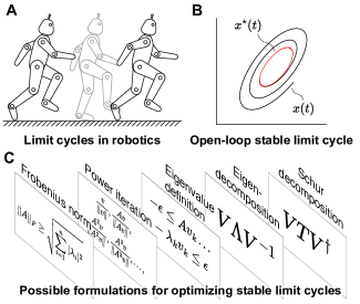
Figure 1: A. Cyclical motions are commonplace in robotics, particularly legged robotics. B. The stability of such cyclical motions ($x(t)$) can be casted in terms of limit cycle stability. Our approach designs a stable limit cycle ($x^{*}(t)$) in a robot via fast and reliable optimization. C. Multiple options for constraining and maximizing stability in numerical trajectory optimizations, which this paper presents and benchmarks for accuracy of stability prediction and computational speed.

In this paper, we cast the open-loop stability problem as a single-stage trajectory optimization problem with explicit stability constraints, and we transcribe it into a nonlinear program using Direct Collocation, which is a fast, reliable, and scalable technique for nonlinear optimization [2] [14]. By allowing for stability to be explicitly formulated, our approach does away with the need to think up a clever way to encode stability implicitly for a given system – e.g., in terms of the post-impact states for bipedal robots – and thus, it is easily applicable to a wide variety of dynamical systems. Also, since limit cycle stability is formulated in terms of eigenvalues, which can be specified rigorous bounds on, both loose and tight, in a number of ways, our method allows one to achieve different trade offs in the solution of the optimization problem; e.g. how fast it is obtained vs. how accurate. In fact, the eigenvalue problem formulations proposed here also generalize to asymptotic stability criteria other than limit cycle stability. For example, one can obtain an asymptotically unstable fixed point of $\dot{x}=f(x)$ by constraining the eigenvalues of the linearized dynamics $\partial f/\partial x$ to the open right-half plane using the formulations we propose. This generalizability to a variety of dynamical systems and notions of stability, the ease with which these notions can be defined as constraints/objectives, and the computational efficiency afforded by our single-loop optimization strategy paired with the analytical tractability of a directly collocated formulation, is what distinguishes our approach from the rest.

II Theoretical Background

A limit cycle is a closed trajectory in state space that has no neighbouring closed trajectories [27]. Finding these cycles is important to design of legged robots, as stable limit cycles find extensive use in engineering stable robotic gaits [7] [10] [12]. In Section III, we describe our approaches to finding stable limit cycles, but here, let us formulate the idea of limit cycle stability as well as present a reformulation that reveals an alternate method to compute it.

We formalize the idea of limit cycle stability in Poincaré’s footsteps. Consider a differential equation

$$\frac{dx}{dt}=f(x),$$ (1)

where $x:[0,\infty)\to\mathbb{R}^{n}\text{, s.t. }x\in\bigcup_{k\geq 2}C^{k}$, is a periodic solution that can be thought of as originating from a codimension-one surface $\mathcal{P}$ – a Poincaré section – of the $n$-dimensional phase space $\mathbb{R}^{n}$. The surface $\mathcal{P}$ is set up so that the flow cuts it traversely, i.e., the normal to $\mathcal{P}$ at $x_{0}\coloneqq x(0)$, $n_{\mathcal{P}}(x_{0})$, satisfies $\langle n_{\mathcal{P}}(x_{0})\,,f(x_{0})\rangle\neq 0$, where $\langle\cdot,\cdot\rangle$ denotes the inner product on $\mathbb{R}^{n}$. Since $x$ is a periodic solution to (1), there exists $\tau:\mathbb{N}\to\mathbb{R}^{+}$ such that if $x_{k}=x(\tau(k))$, then $x_{k}\in\mathcal{P}$. The $(n-1)$-dimensional discrete dynamical system $\phi_{\mathcal{P}}:\mathcal{P}\to\mathcal{P}$ such that $\phi_{\mathcal{P}}(x_{k-1})=x_{k}$, called the Poincaré map, encodes the transverse dynamics that describe how the trajectories “near” $x$ behave.

every picture/.style=line width=0.75pt

[x=0.675pt,y=0.675pt,yscale=-0.6,xscale=0.6]

[draw=rgb, 255: red, 0; green, 0; blue, 0 , fill=rgb, 255: red, 135; green, 186; blue, 226 ,fill opacity=0.6 ] (135.88,64.35) – (209.29,18.91) – (206.9,155.16) – (133.5,200.6) – cycle ; [fill=rgb, 255:red, 0; green, 0; blue, 0 ,fill opacity=1 ] (166.28,103.17) .. controls (166.28,101.51) and (167.63,100.17) .. (169.28,100.17) .. controls (170.94,100.17) and (172.28,101.51) .. (172.28,103.17) .. controls (172.28,104.82) and (170.94,106.17) .. (169.28,106.17) .. controls (167.63,106.17) and (166.28,104.82) .. (166.28,103.17) – cycle ; [color=rgb, 255:red, 0; green, 0; blue, 0 ][line width=0.75] [line join = round][line cap = round] (169,104.27) .. controls (334,120) and (303,221) .. (160,221) .. controls (1,222) and (13,122.33) .. (133,124.15) ; [line width=0.75] [dash pattern=on 4.5pt off 4.5pt] (133,124.15) – (169,126.33) ; [fill=rgb, 255:red, 0; green, 0; blue, 0 ,fill opacity=1 ] (166,126.33) .. controls (166,124.68) and (167.34,123.33) .. (169,123.33) .. controls (170.66,123.33) and (172,124.68) .. (172,126.33) .. controls (172,127.99) and (170.66,129.33) .. (169,129.33) .. controls (167.34,129.33) and (166,127.99) .. (166,126.33) – cycle ; (169,230.33) – (151,220.5) – (169,210.67) ;

(216,23.4) node [anchor=north west][inner sep=0.75pt] $\mathcal{P}$; (172,78.4) node [anchor=north west][inner sep=0.75pt] $x_{k}$; (140,138.4) node [anchor=north west][inner sep=0.75pt] $x_{k+1}$;

every picture/.style=line width=0.75pt [x=0.675pt,y=0.675pt,yscale=-0.6,xscale=0.6] [draw=rgb, 255: red, 0; green, 0; blue, 0 , fill=rgb, 255: red, 135; green, 186; blue, 226 ,fill opacity=0.6 ] (121.48,66.46) – (194.88,21.02) – (192.5,157.26) – (119.09,202.7) – cycle ; [draw opacity=0] (158.69,103.17) .. controls (220.59,103.79) and (270.39,129.4) .. (270.39,160.9) .. controls (270.39,192.8) and (219.35,218.65) .. (156.39,218.65) .. controls (93.43,218.65) and (42.39,192.8) .. (42.39,160.9) .. controls (42.39,136.7) and (71.79,115.98) .. (113.48,107.39) – (156.39,160.9) – cycle ; (158.69,103.17) .. controls (220.59,103.79) and (270.39,129.4) .. (270.39,160.9) .. controls (270.39,192.8) and (219.35,218.65) .. (156.39,218.65) .. controls (93.43,218.65) and (42.39,192.8) .. (42.39,160.9) .. controls (42.39,136.7) and (71.79,115.98) .. (113.48,107.39) ; [draw opacity=0][dash pattern=on 4.5pt off 4.5pt] (158.69,103.17) .. controls (220.59,103.79) and (270.39,129.4) .. (270.39,160.9) .. controls (270.39,192.8) and (219.35,218.65) .. (156.39,218.65) .. controls (93.43,218.65) and (42.39,192.8) .. (42.39,160.9) .. controls (42.39,129.01) and (93.43,103.16) .. (156.39,103.16) .. controls (157.16,103.16) and (157.92,103.16) .. (158.68,103.17) – (156.39,160.9) – cycle ; [dash pattern=on 4.5pt off 4.5pt] (158.69,103.17) .. controls (220.59,103.79) and (270.39,129.4) .. (270.39,160.9) .. controls (270.39,192.8) and (219.35,218.65) .. (156.39,218.65) .. controls (93.43,218.65) and (42.39,192.8) .. (42.39,160.9) .. controls (42.39,129.01) and (93.43,103.16) .. (156.39,103.16) .. controls (157.16,103.16) and (157.92,103.16) .. (158.68,103.17) ; [fill=rgb, 255:red, 0; green, 0; blue, 0 ,fill opacity=1 ] (155.28,103.17) .. controls (155.28,101.51) and (156.63,100.17) .. (158.28,100.17) .. controls (159.94,100.17) and (161.28,101.51) .. (161.28,103.17) .. controls (161.28,104.82) and (159.94,106.17) .. (158.28,106.17) .. controls (156.63,106.17) and (155.28,104.82) .. (155.28,103.17) – cycle ; (168,228.33) – (150,218.5) – (168,208.67) ; (203,23.4) node [anchor=north west][inner sep=0.75pt] $\mathcal{P}$; (149,114.4) node [anchor=north west][inner sep=0.75pt] $x_{0}^{*}$;

Figure 2: A. Periodic curve cutting a Poincaré surface $\mathcal{P}$ in $\mathbb{R}^{3}$. B. Limit cycle corresponding to fixed point $x_{0}^{*}\in\mathbb{R}^{3}$ of the Poincaré map $\phi_{\mathcal{P}}$.

Say $x^{*}:[0,\infty)\to\mathbb{R}^{n}$ is a periodic solution to (1) such that $x^{*}_{0}\in\mathcal{P}$ and $x_{k}^{*}=\phi(x_{k-1}^{*})=x_{k-1}^{*}$. Then, $x^{*}_{k}$ is a fixed point of the Poincaré map $\phi_{\mathcal{P}}$, and we say that it is stable inside a neighbourhood $\mathcal{U}\subset\mathcal{P}$ if for all periodic solutions $x$ to (1) such that $x_{0}\in\mathcal{U}$, $\lim_{k\to\infty}x_{k}=x^{*}_{0}$. Now, suppose $\eta_{k}$ is the distance between $x^{*}$ and a “nearby” trajectory $x$ at the $k^{\text{th}}$ Poincaré section “intersection”. Then

$$\eta_{k}=\frac{\partial\phi_{\mathcal{P}}}{\partial x}\bigg{\rvert}_{x^{*}_{0}}\eta_{k-1}$$

to the first order [28]. We can see that $x^{*}_{0}$ is stable if $\eta_{k}\to 0$ as $k\to\infty$, i.e., if the eigenvalues of $\partial\phi_{\mathcal{P}}(x_{0}^{*})/\partial x$ lie inside the unit circle in $\mathbb{C}$. Notice that if $x^{*}_{0}$ is a fixed point of the Poincaré map $\phi_{\mathcal{P}}$, then the corresponding trajectory $x^{*}$ is a limit cycle (Figure 2). One may thus define a limit cycle $x^{*}$ as stable if the corresponding fixed point $x^{*}_{0}$ of the discrete map $\phi_{\mathcal{P}}$ is stable. This definition of stability makes intuitive sense: it describes whether trajectories in a neighbourhood $\mathcal{U}^{\prime}\subset\mathbb{R}^{n}$ of the limit cycle asymptotically converge to it. And this intuition leads us to an alternate procedure for evaluating the stability of a limit cycle. Say $x^{*}$ is a limit cycle of (1) and $x^{*}+\delta x$ is a trajectory in a neighbourhood $\mathcal{U}^{\prime}\subset\mathbb{R}^{n}$ of $x^{*}$. One can see that after one period, the difference, $\delta x$, between $x^{*}$ and $x^{*}+\delta x$ is given to the first order by

$$\delta x(T)=\frac{\partial x^{*}}{\partial x_{0}}\bigg{|}_{T}\delta x(0),$$

where $T$ is the period [26]. Clearly, the matrix $\mathcal{M}(T)=\partial x^{*}(T)/\partial x_{0}$ governs whether the perturbation $\delta x(0)$ decays and the perturbed trajectory converges to the limit cycle. This matrix is called the monodromy matrix, and notice that it is the solution at time $T$ to the variational equation

$$\frac{d\mathcal{M}}{dt}=\frac{\partial f}{\partial x}\bigg{\rvert}_{x^{*}}\mathcal{M},\quad\mathcal{M}(0)=I_{n\times n}.$$ (2)

Thus, one may integrate (2) over the period $T$ of the limit cycle, and check whether the eigenvalues of $\mathcal{M}(T)$ lie inside the unit circle in $\mathbb{C}$ to find out if the limit cycle $x^{*}$ is stable.

III Methods

We pose the problem of finding an open-loop stable limit cycle as the following optimization problem:

$$\min_{u,T,\mathcal{I}_{k}}\,\int_{0}^{T}\!J(x(t),u(t))\,dt$$ (3)

$$\text{s.t. }\forall\,t\in\mathcal{I}_{k}\quad\dot{x}(t)=f_{k}(x(t),u(t),\psi_{k}),$$ (4)

$$\quad\quad\quad\quad\,\,\quad\,\,\,g(x(t),u(t))\equiv 0,$$ (5)

$$\quad\quad\quad\quad\,\,\quad\,\,\,h(x(t),u(t))\succcurlyeq 0,$$ (6)

where $\mathcal{I}_{k}$ implicitly defines the phases based on the phase boundaries determined by the complex-valued vector functions $g$ and $h$, where we define $g\equiv a+bi$ as $\Re(g)\equiv a$ and $\Im(g)\equiv b$, and $h\succcurlyeq a+bi$ as the relational identities $\Re(h)\geq a$ and $\Im(h)\geq b$. The functions $g$ and $h$ also include other constraints, particularly, periodicity and limit cycle stability:

$$g_{lc}=x(T)-x(0)$$ (7)

$$h_{st}={-|\lambda_{i}(\mathrm{X})|}+\rho_{\text{max}}\quad\forall\,i\in\{1,\dots,n\}$$ (8)

where $\rho_{\text{max}}$ is the desired bound on the magnitude of the eigenvalues of $\mathrm{X}\in\mathbb{R}^{n\times n}$, which may be the matrix $\partial\phi(x_{0}^{*})/\partial x$ or $\mathcal{M}(T)$. In the case of $\mathrm{X}=\mathcal{M}(T)$, we need to add (2) too as a PDE constraint for each $f_{k}$.

III-A Bounding spectral radius

As discussed in Section II, for the cycle $x^{*}$ to be stable, we must set $\rho_{\text{max}}<1$ in (8). However, bounding $h_{st}\geq 0$ is not trivial. This subsection discusses the complication, and presents the approaches we have formulated to that end.

The set $\mathcal{E}(A)=\{\lambda_{i}(A)\}_{i=1}^{m}$ of all eigenvalues of a matrix $\mathrm{A}\in\mathbb{R}^{m\times m}$ is called its spectrum; and its spectral radius, denoted $\rho(A)$, is defined to be the magnitude of the largest eigenvalue: $\rho(\mathrm{A})\!=\!\max\{|\lambda_{i}(A)|\}_{i=1}^{m}$. One can see that to define the constraint $h_{st}\geq 0$, it suffices to bound $\rho(\mathrm{X})\leq\rho_{\text{max}}$. However, bounding the spectral radius of an arbitrary real matrix is difficult, and most of the previous work in this line has assumed some special structure on the matrices, especially symmetry, because the eigenvalues of symmetric matrices are Lipchitz functions of their elements (Lidskii’s theorem), which makes semidefinite programming a viable approach to bounding/optimizing the spectral radius [16] [15]. For non-symmetric matrices – in particular, for the matrices $\partial\phi(x_{0}^{*})/\partial x$ and $\mathcal{M}(T)$ – the spectral radius is a non-Lipschitz function of matrix elements [16]. And not only that, the matrices $\partial\phi(x_{0}^{*})/\partial x$ and $\mathcal{M}(T)$ are also unknown as nonlinear functions of the optimization variables. For such matrices, the previous approaches to bounding spectral radius fail, and furthermore, our investigations reveal that bounding the spectral radius of such matrices using general formulations of the eigenvalue problem result in difficult-to-solve CSPs. For example, one can constrain $\rho(X)\leq\rho_{\text{max}}$, where $X$ can be either of $\partial\phi(x_{0}^{*})/\partial x$ or $\mathcal{M}(T)$, by using a computer algebra system [13] to compute the symbolic formulation of $\text{det}\,X-\lambda I$, and adding scalar constraints to the optimization problem that bound the magnitude of the roots of this polynomial:

$$|\lambda|\,\leq\,\rho_{\text{max}}\,\,\,\,\forall\,\lambda\,\,\text{ s.t. }{-\epsilon}\leq\text{det}\,X-\lambda I\leq\epsilon.$$

However, we found that this approach scaled poorly with the size of $X$, because $\text{det}\,X-\lambda I$ gets very involved as X grows in size. To get a better conditioned formulation, we directly casted $Xv=\lambda v$, where $v$ is the eigenvector corresponding to the eigenvalue $\lambda$ of $X$, as a CSP inside the NLP:

Find $\lambda_{i}\in\mathbb{C}$ and $v_{i}\in\mathbb{C}^{n}$ such that

$${-\epsilon}\leq Xv_{i}-\lambda_{i}v_{i}\leq\epsilon$$ (9)

$$\lambda_{i}-\lambda_{i-1}\geq\epsilon$$ (10)

$${-1}+\epsilon\leq v_{i}^{T}v_{i-1}\leq 1-\epsilon$$ (11)

However, we discovered that this CSP was also difficult to solve, because of the discontinous nature of the solution landscape, as shown in Fig. 3A. We also noticed that “patches” to this CSP (see 3B) to facilitate the solver in navigating the solution landscape resulted in a significant computational overhead in high-dimensional eigenvalue problems. To make a long story short, our observation has been that naïve general formulations of the eigenvalue problem result in ill-conditioned CSPs for constraining the spectral radii of $\partial\phi(x_{0}^{*})/\partial x$ and $\mathcal{M}(T)$. Specalized formulations of the eigenvalue problem, i.e., formulations that hold only for certain $\partial\phi(x_{0}^{*})/\partial x$ and $\mathcal{M}(T)$, result in CSPs that are more numerically stable. These specalized CSPs and the conditions under which they hold have been developed in sections III-B - III-D. In section III-E, we develop a fairly general CSP formulation of the eigenvalue problem using Schur Decomposition, which applies to a wider range of problems, unlike specialized CSPs, and is efficient (though not efficient as specialized CSPs, where they apply).

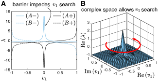
Figure 3: A. The constraint landspace of the $2$D eigenvalue problem:
$\phantom{.}\hskip 15.0ptAv=\lambda v,\hskip 2.0pt\text{ where }A=\begin{bmatrix}a_{11}&a_{12}\\[-3.00003pt] a_{21}&a_{22}\end{bmatrix}\in\mathbb{R}^{n\times n},\,v=\begin{bmatrix}v_{1}\\[-3.00003pt] v_{2}\end{bmatrix}\in\mathbb{R}^{2}$
The optimization variables $\lambda$ and $v_{1}$ here have been constrained to the real-line. It can be seen that the discontinuity at $v_{1}=0$ can throw off gradient-based search methods. B. The curve labeled $A-$ in A lifted to $\mathbb{C}^{2}$ from $\mathbb{R}^{2}$ by allowing $\lambda,v_{1}$ to be complex values, even though the $\lambda$ and $v_{1}$ that solve this eigenvalue problem are real-valued. The solver may be guided towards real-valued solutions through a regularization objective, $\min_{\lambda_{i}}\,{-k}\left(\Im\left(\lambda_{1}\right)+\Im\left(\lambda_{2}\right)\right)$. The introduction of extra dimensions to the solution space serves to condition the problem: it allows the solver to circumvent the discontinuities along the real axes by moving along the imaginary axes. However, this way of “patching” the CSP by lifting the constraints to a high-dimensional space does not scale well to cases where the problem is already high-dimensional.

III-B Bounding spectral radius through the Frobenius norm

The Frobenius norm of a real matrix $X$, denoted $\|X\|_{F}$, is the squareroot of the sum of the squares of its elements, and it is an upper bound on the squareroot of the sum of the squares of the magnitudes of the eigenvalues of $X$ [11]:

$$\|X\|_{F}=\,\sqrt{\sum_{i=1}^{n}\sum_{j=1}^{n}x_{ij}^{2}}\geq\sqrt{\sum_{i=1}^{n}|\lambda_{i}(X)|^{2}}$$

Thus, bounding $\|X\|_{F}$ bounds $\rho(X)$, and since $\|X\|_{F}$ is a differentiable function of simply the matrix elements, $x_{ij}$, the resulting CSP is well-conditioned. However, note that $\|X\|_{F}$ is a conservative upper bound on $\rho(X)$, and thus, in cases where $|\rho(X)-\rho_{\max}|\ll 1$, the loose Frobenius norm based constraint may make it difficult to find a solution to the NLP. But outside of these cases, the Frobenius norm based bound on the spectral radius should be one’s first consideration from among all the methods we propose.

III-C Defining the dominant eigenvalue using Power Iteration

Power Iteration is a numerical algorithm for computing the dominant eigenvalue of a matrix, i.e., the eigenvalue $\lambda_{1}\in\mathcal{E}(X)$ s.t. $|\lambda_{1}|\,=\rho(X)$. The iteration is given by the sequence

$$\frac{v}{\|v\|},\frac{Av}{\|Av\|},\frac{A^{2}v}{\|A^{2}v\|},\frac{A^{3}v}{\|A^{3}v\|},\dots,$$

which, under certain assumptions, can be shown to converge to the eigenvector $v_{1}$ corresponding to $\lambda_{1}$ [30]:

$$\lim_{k\to\infty}{A^{k}v}/{\|A^{k}v\|}={v_{1}}/{\|v_{1}\|}$$

For computation, one can formulate power iteration as the recursion $v^{(k+1)}={Av^{(k)}}/{\|Av^{(k)}\|},$ which can then further be broken down into two separate recursions:

$$w^{(k+1)}=Av^{(k)},\hskip 10.0ptv^{(k+1)}={w^{(k+1)}}/{\|w^{(k+1)}\|}$$

This recursive formulation of power iteration gives rise to the following CSP for finding the dominant eigenvalue:

Find $\lambda\in\mathbb{R}$, $v\in\mathbb{R}^{n}$ subject to

$$v^{(n+1)}=Av^{(n)}$$ (12)

$$1-\epsilon\leq\|v^{(n+1)}\|\leq 1+\epsilon$$ (13)

$${-\epsilon}\leq\lambda-(v^{(n+1)})^{T}Xv^{(n+1)}\leq\epsilon$$ (14)

The superscript on $v$ indicates the node number in Direct Collocation. Note that the constraint in (13) is necessary for numerical stability in the case where $X$ is an unstable matrix, i.e., $\lim_{k\to\infty}X^{k}$ is undefined. However, unstable matrices are not the only limitation of the power iteration method. In particular, power iteration assumes that $\lim_{k\to\infty}{A^{k}v}/{\|A^{k}v\|}$ exists, i.e., $\lambda_{1}$ is strictly greater than the next “largest” eigenvalue of $A$: $|\lambda_{1}/\lambda_{2}|>\!1$ [30]. This means that the power iteration method would fail if $\lambda_{1}\in\mathbb{C}$, since $\lambda_{1}\in\mathbb{C}$ implies $\lambda_{2}=\overline{\lambda_{1}}$, and thus $|\lambda_{1}/\lambda_{2}|=\!\!1$. However, for problems where the matrix is stable and is known to have a real dominant eigenvalue, the power iteration method can be a fast and reliable approach to bound the spectral radius.

III-D Defining eigenvalues through eigendecomposition

A diagonalizable real matrix $A\in\mathbb{R}^{n\times n}$ can be decomposed as $A=V\Lambda V^{-1}$, where

$$\Lambda=\begin{bmatrix}\lambda_{1}&&\\[-11.99998pt] &\ddots&\\[-6.99997pt] &&\lambda_{n}\end{bmatrix},\hskip 5.0ptV=\begin{bmatrix}|&|&&|\\[-3.99994pt] v_{1}&v_{2}&\dots&v_{n}\\[-1.99997pt] |&|&&|\end{bmatrix},$$

are the matrices containing the eigenvalues and eigenvectors of $A$, respectively, i.e., $Av_{i}=\lambda_{i}v_{i}$ [29]. The eigendecomposition of a matrix can be formulated as a CSP as follows:

Find $\Lambda$, $V$, $V^{-1}\in\mathbb{C}^{n\times n}$ such that

$$-\epsilon\leq A-V\Lambda V^{-1}\leq\epsilon$$ (15)

$$-\epsilon\leq I-VV^{-1}\leq\epsilon$$ (16)

Notice that even if $A$ is a defective matrix, i.e., $\lambda_{i}=\lambda_{j}$ and $v_{i}=\alpha v_{j}$ for some $i$ and $j$, the “wiggle room” defined by $\epsilon$ in the above CSP can still allow us to decompose the matrix and compute the eigenvalues. The shortcoming of this method, however, is that the above CSP is slow to solve. This can be alleviated by restating $A=V\Lambda V^{-1}$ as $AV=V\Lambda$, thus getting rid of the constraint in (16):

Find $\Lambda$, $V\in\mathbb{C}^{n\times n}$ such that

$$-\epsilon\leq AV-V\Lambda\leq\epsilon$$ (17)

This CSP is often the fastest to solve when the other specialized CSPs are not suitable, however, the loose nature of it allows the solver to “cheat”, by setting:

$$\Lambda=\begin{bmatrix}\lambda_{j}&&\\[-11.99998pt] &\ddots&\\[-6.99997pt] &&\lambda_{j}\end{bmatrix},\hskip 5.0ptV=\begin{bmatrix}|&|&&|\\[-3.99994pt] v_{j}&v_{j}&\dots&v_{j}\\[-1.99997pt] |&|&&|\end{bmatrix},\hskip 5.0ptj\in\{2,\dots,n\}$$

In such a case, one may try different initial guesses for $\Lambda$ and $V$, but this trail-and-error process can be a rather significant amount of manual labour.

III-E Defining eigenvalues through Schur Decomposition

Schur Decomposition, $X=VTV^{\dagger}$, where $T$ is an upper-triangular matrix, is a decomposition of a real matrix $X$ into its eigenvalues [29]. This method lends itself to a widely-applicable yet relatively fast-solving CSP formulation of the eigenvalue problem:

Find $T\in\mathcal{Q}^{n\times n}$, $V\in\mathbb{C}^{n\times n}$ subject to

$$-\epsilon\leq VV^{\dagger}-I\leq\epsilon$$ (18)

$$-\epsilon\leq X-VTV^{\dagger}\leq\epsilon$$ (19)

where $\mathcal{Q}^{n\times n}=\{U\in\mathbb{C}^{n\times n}\,|\,U_{ij}=0\,\,\,\forall\,j<i\}$.

We can make the formulation better conditioned through algebraic manipulation of the expressions and introduction of explicit Linear Algebra based constrains:

Find $V$, $V^{-1}$, $T\in\mathbb{C}^{n\times n}$ subject to

$$-\epsilon\leq VV^{-1}-I\leq\epsilon$$ (20)

$$-\epsilon\leq V^{-1}-V^{\dagger}\leq\epsilon$$ (21)

$$-\epsilon\leq X-VTV^{-1}\leq\epsilon$$ (22)

$$T_{ij}=0\,\,\text{ for all }j<i$$ (23)

In cases where the specialized CSPs from III-B-III-D apply, their use should be preferred, as they are almost always faster to solve than the formulation above. The novelty of this formulation is that it is general (and hence applicable to a variety of systems and tasks) yet numerically stable and relatively fast-solving (compared to the other general formulations of the eigenvalue problem).

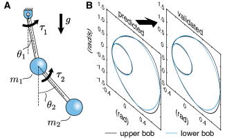
Figure 4: A. Robot swing-leg modeled as a double pendulum with actuated joints and viscous damping. In our experiments, we set $m_{1}\!\!=\!\!m_{2}\!\!=\!\!1\,\text{kg}$, and $L_{1}\!\!=\!\!L_{2}\!\!=\!\!1\,\text{m}$. B. A stable limit cycle of a moderately damped double pendulum predicted by stability-constrained optimization with an energy minimization objective. The stability of the limit cycle is validated by simulating the system from a point close to the cycle.

IV Experiments and Results

We now present experiments based on our proposed approach. First, we provide a comprehensive analysis comparing the different methods we introduced in the context of swing-leg stabilization. Subsequently, we showcase our methodology in achieving stable hopping in a spring-loaded inverted pendulum (SLIP) model in different scenarios.

IV-A Swing-leg stabilization

Computing an open-loop stable limit cycle of a robot’s swing-leg is a non-trivial control problem, and it thus serves as a good benchmark for the stability-constrained optimization methods presented here. We model swing-leg as a double pendulum, as shown in Fig. 4A, and formulate its equations of motion as:

$$(m_{1}+m_{2})L_{1}\ddot{\theta}_{1}+m_{2}L_{2}\ddot{\theta}_{2}\cos(\theta_{1}-\theta_{2})+(m_{1}+m_{2})gsin\theta_{1}\\ +m_{2}L_{2}\dot{\theta}_{2}^{2}\sin(\theta_{1}-\theta_{2})+b_{1}\dot{\theta}_{1}=\tau_{1}\quad$$

$$m_{2}L_{2}\ddot{\theta}_{2}+m_{2}L_{1}\ddot{\theta}_{1}\cos(\theta_{1}-\theta_{2})-m_{2}L_{1}\dot{\theta}_{1}^{2}\sin(\theta_{1}-\theta_{2})\\ +m_{2}g\sin\theta_{2}+b_{2}\dot{\theta}_{2}=\tau_{2}\quad\quad\quad$$

These have been obtained by minimizing the action functional, $\mathcal{S}[\theta_{1},\theta_{2}]:=\int_{0}^{t}L(\theta_{1},\dot{\theta}_{1},\theta_{2},\dot{\theta}_{2},t)dt,$ where $L$ is the Lagrangian of the system [9].

Through our experiments on various configurations of the double pendulum system, we have come to find the monodromy matrix method (where $X\!=\!\mathcal{M}(T)$) to be more reliable than the Poincaré method (where $X\!\!=\!\partial\phi(x_{0}^{*})/\partial x$) for stability-constrained optimization. For the case with moderate damping ($b_{1}\!\!=\!\!b_{2}\!\!=\!3.75\,\text{Ns/m}$), both the methods performed well. In fact, we got the same limit cycle (shown in Fig. 4B) from both the optimizations, and it was stable. We validated the stability of the limit cycle by simulating the double pendulum from a point close to the limit cycle and confirming that the trajectory got closer to the limit cycle over time. However, for the case with low damping ($b_{1}\!\!=\!\!b_{2}\!\!=\!0.18\,\text{Ns/m}$), shown in Fig. 5, the Poincaré method based optimization failed: the limit cycle it gave as stable, when simulated, came out to be unstable. We believe this to be due to numerical inaccuracies in computing the Jacobian of the return map in the Poincaré method. Also, the Poincaré method is sensitive to the placement of the Poincaré section, and a different placement of the Poincaré section may give a different result.

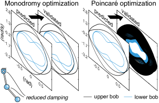
Figure 5: Stability-constrained optimization using the Poincaré method based definition of stability sometimes gives unstable limit cycles. This figure shows such a case, where we have a lightly damped double pendulum modeling a swing-leg. Left. A stable limit cycle predicted by the monodromy matrix based optimization. Right. A stable limit cycle predicted by the Poincaré method based optimization. When the stability of this limit cycle is validated through simulation, we see that it is actually unstable, since the neighbouring trajectories diverge from it.

	Section	$\lambda_{\max}(\mathcal{M}(T))$	Time (s)
Frobenius Norm	III-B	0.6198 + 0.2778i	49.8
Power Iteration	III-C	0.7876 + 0.0509i	345.77
Eigenvalue Definition	III-A	0.8837 + 0.0958i	287.87
Eigendecomposition	III-D	0.7875 + 0.0493i	242.81
Schur Decomposition	III-E	0.7875 + 0.0493i	73.96
Symbolic Method	III-A	N/A	N/A

TABLE I: Dominant eigenvalues of $\mathcal{M}(T)$ corresponding to the limit cycles in Fig. 6, and the time taken to compute the limit cycles. The ”N/A” in the last row shows that the optimization based on the symbolic method for eigenvalue computation was unable to converge.

In Fig. 6, we show how the various methods we presented in III-A-III-E for constraining spectral radius perform at stability-constrained optimization of the double pendulum with low damping. All the limit cycles in Fig. 6 have been obtained against a strict stability constraint, $\rho(\mathcal{M}(T))\leq 1-\epsilon$, and an energy minimization objective:

$$J=\int_{0}^{T}\tau_{1}^{2}+\tau_{2}^{2}\,dt,$$

where $T$ is the time period of the limit cycle. The first plot in Fig. 6 shows the limit cycle obtained when the stability constraint is enforced through the Frobenius norm: $\|\mathcal{M}(T)\|_{F}\leq 1$. The first row in TABLE 1 gives the dominant eigenvalue of $\mathcal{M}(T)$ corresponding to this limit cycle. Notice that the absolute value of the dominant eigenvalue is $0.6792$, which is considerably lesser than $1$, the largest spectral radius of $\mathcal{M}(T)$ against which the system can be stable. As we explained, this is because the Frobenius norm is not a tight constraint on the dominant eigenvalue. But notice that, on the upside, the optimization problem was solved the fastest.

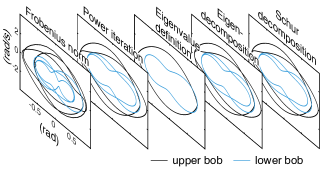
Figure 6: This figure show the limit cycles obtained from stability-constrained optimization of swing-leg using the various eigenvalue computation methods presented in this work.

When the spectral radius of $\mathcal{M}(T)$ is bounded using the power iteration method, we get a stable limit cycle that appears very different from the one obtained using the Frobenius norm constraint, as can be seen seen in Fig. 6. The dominant eigenvalue for $\mathcal{M}(T)$ corresponding to this limit cycle, given in TABLE 1, has an absolute value of $0.7935$, which indicates that the power iteration formulation allows for a much tighter bound on the dominant eigenvalue. Notice that the dominant eigenvalue is complex, yet the power iteration method gave a solution. This is because the imaginary part of the dominant eigenvalue is relatively small. The power iteration method only finds solutions where $\Im\left(\lambda_{\max}(\mathcal{M}(T))\right)\approx 0$. This reveals a particularly useful feature of the power iteration method, as it can be used in applications where one desires real (or “almost real”) solutions to the eigenvalue problem.

The third plot in Fig. 6 shows the limit cycle obtained by using the eigenvalue definition method to define the constraint $\rho(\mathcal{M}(T))\leq 1$. The dominant eigenvalue of $\mathcal{M}(T)$ for this limit cycle has a magnitude of $0.8889$. Of all the limit cycles in Fig. 6, this one has the largest spectral radius of the associated monodromy matrix. But this is not a consistent behavior, and it may be attributed to the initial guesses supplied to the optimization, among other factors.

The forth limit cycle in Fig. 6 has been obtained using the eigendecomposition based spectral radius constraints. Notice that this is the same limit cycle as the one obtained using the Power Iteration method. The Schur decomposition method also gives this exact same limit cycle, as shown in the last plot of Fig. 6. However, the Schur decomposition was the fastest to converge after the Frobenius Norm based method in this case, and required minimum tuning of the initial guesses.

IV-B Stabilization of SLIP model in template-based control

The spring-loaded inverted pendulum (SLIP) model is a reduced-order model of dynamic gaits observed in nature. Because of its computational and mechanical tractability, it is commonly employed for template-based control of walking systems [1] [23]. However, the hybrid nature of the SLIP model, involving frequent switches between dynamical models, can pose a challenge for gradient-based optimization methods. In this section, we demonstrate how our approach robustly generates stable open-loop controllers for hybrid dynamical systems in a short amount of time.

To generate open-loop stable hopping in a SLIP model (Fig. 7A), we use the monodromy matrix based criteria for stability evaluation and compute the spectral radius of the monodromy matrix using the Schur decomposition. The input to the system is the rate at which the actuator length, $l_{a}$, changes, and the dynamics are described by the hybrid system

$$\ddot{z}_{m} =\frac{k}{m}\Big{(}l_{a}-l\Big{)}+\frac{c}{m}\left(\dot{l}_{a}-\dot{l}\,\right)\!-g \text{if }z_{m}=0$$

$$\ddot{z}_{m} \equiv{-g}$$ otherwise

where $l(t)=z_{m}(t)-z_{\text{toe}}(t)$ is the length of the robot. The dynamic and kinematic parameters of the robot have been chosen to mimic biological bipeds [3].

Fig. 7B-D shows the results of stability-constrained optimization of the actuated SLIP model with various task and input constraints:

$$\text{(a) }\,\,\,l(t)\leq 1.1\,\,\forall t,$$

$$\text{(b) }\,\,\,0\leq F_{\text{net}}(t)\leq 3\,\,\forall t,\text{ and}$$

$$\text{(c) }\,\,\,\int_{0}^{T}F_{\text{net}}(t)\,dt\geq 0.5,\,\,\text{ where }T\geq 1$$

It can be seen in Fig. 7B that constraining the spectral radius of the mondoromy matrix to be no larger than 1 gives an egg-shaped limit cycle. The optimization took less than $2$ seconds to find this limit cycle, and it is stable, with $\lambda_{\max}(\mathcal{M}(T))\!\!\!=\!\!\!{-0.3263}+0.7846i$. The simulation result confirms the stability of this limit cycle, as the system converges to the limit cycle when started from a point close to it. Fig. 7C shows the limit cycle obtained when the spectral radius of the monodromy matrix is constrained to less than $0.7$. This limit cycle has $\lambda_{\text{max}}(\mathcal{M}(T))=0.5283+0.3555i$. The limit cycle in Fig. 7D is also obtained against the same spectral radius constraint, however, in this case, we had an energy-minimization objective in the optimization. For this cycle, we got $\lambda_{\text{max}}(\mathcal{M}(T))=0.5180+0.3716i$, and the simulation indeed confirms that it is a stable limit cycle.

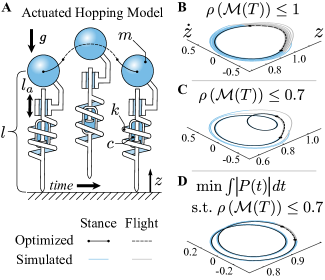
Figure 7: A. The actuated spring-loaded inverted pendulum (SLIP) model with a damper for template-based control of legged robots. B, C, D. The result of simulating the SLIP model from an initial state close to a limit cycle (colored black). In B, the limit cycle has been obtained using stability-constrained optimization with the spectral radius of the monodromy matrix constrained to less than 1. The limit cycles in C and D have been obtained by bounding the spectral radius to less than 0.7, however, in D, we also have an energy minimization objective.

V Conclusion

We posed open-loop limit cycle stability as a trajectory optimization problem using two different methods: the mondromy matrix method, and Poincaré method. We developed various CSP formulations of the eigenvalue problem for efficiently bounding the spectral radii of the matrices involved in these methods. Our experiments on the damped double pendulum model for robotic swing-leg demonstrate that the monodromy matrix method is more reliable for defining limit cycle stability in optimization than the Poincaré method. Furthermore, our findings suggest that specialized CSP formulations of the eigenvalue problem are highly effective for stability-constrained optimization when applicable. In cases where they do not apply, the Schur decomposition-based formulation strikes a good balance between numerical stability and computational tractability.

Using our approach for stability-constrained optimization, we show that we successfully generate a controller for open-loop stable hopping in a SLIP-templated robot in under 2 seconds. Future work may focus on investigating more complex legged systems for stability-constrained optimization. Furthermore, work on improving the eigenvalue CSPs and discovering new ones may lead to potential speed ups and numerical stability.

References

- [1] Taylor Apgar, Patrick Clary, Kevin Green, Alan Fern, and Jonathan W Hurst. Fast online trajectory optimization for the bipedal robot cassie. In Robotics: Science and Systems, volume 101, page 14, 2018.
- [2] John T Betts. Survey of numerical methods for trajectory optimization. Journal of guidance, control, and dynamics, 21(2):193–207, 1998.
- [3] Aleksandra V Birn-Jeffery, Christian M Hubicki, Yvonne Blum, Daniel Renjewski, Jonathan W Hurst, and Monica A Daley. Don’t break a leg: running birds from quail to ostrich prioritise leg safety and economy on uneven terrain. Journal of Experimental Biology, 217(21):3786–3796, 2014.
- [4] Jorge G Cham, Sean A Bailey, Jonathan E Clark, Robert J Full, and Mark R Cutkosky. Fast and robust: Hexapedal robots via shape deposition manufacturing. The International Journal of Robotics Research, 21(10-11):869–882, 2002.
- [5] Michael Jon Coleman. A stability study of a three-dimensional passive-dynamic model of human gait. Cornell University, 1998.
- [6] Hongkai Dai and Russ Tedrake. Optimizing robust limit cycles for legged locomotion on unknown terrain. In 2012 IEEE 51st IEEE Conference on Decision and Control (CDC), pages 1207–1213. IEEE, 2012.
- [7] Hongkai Dai and Russ Tedrake. L 2-gain optimization for robust bipedal walking on unknown terrain. In 2013 IEEE international conference on robotics and automation, pages 3116–3123. IEEE, 2013.
- [8] M. Ernst, H. Geyer, and R. Blickhan. Spring-legged locomotion on uneven ground: A control approach to keep the running speed constant. 2009.
- [9] Louis N Hand and Janet D Finch. Analytical mechanics. Cambridge University Press, 1998.
- [10] Daan GE Hobbelen and Martijn Wisse. A disturbance rejection measure for limit cycle walkers: The gait sensitivity norm. IEEE Transactions on robotics, 23(6):1213–1224, 2007.
- [11] Roger A Horn and Charles R Johnson. Matrix analysis. Cambridge university press, 2012.
- [12] Christian Hubicki, Mikhail Jones, Monica Daley, and Jonathan Hurst. Do limit cycles matter in the long run? stable orbits and sliding-mass dynamics emerge in task-optimal locomotion. In 2015 IEEE International Conference on Robotics and Automation (ICRA), pages 5113–5120. IEEE, 2015.
- [13] The MathWorks Inc. MATLAB and Symbolic Math Toolbox. Natick, Massachusetts, 2017.
- [14] Matthew Kelly. An introduction to trajectory optimization: How to do your own direct collocation. SIAM Review, 59(4):849–904, 2017.
- [15] Adrian S Lewis. The mathematics of eigenvalue optimization. Mathematical Programming, 97(1):155–176, 2003.
- [16] Adrian S Lewis and Michael L Overton. Eigenvalue optimization. Acta numerica, 5:149–190, 1996.
- [17] K Mombaur. Performing open-loop stable flip-flops—an example for stability optimization and robustness analysis of fast periodic motions. In Fast Motions in Biomechanics and Robotics, pages 253–275. Springer, 2006.
- [18] Katja Mombaur. Using optimization to create self-stable human-like running. Robotica, 27(3):321–330, 2009.
- [19] Katja D Mombaur, Hans Georg Bock, and RW Longman. Stable, unstable and chaotic motions of bipedal walking robots without feedback. In 2000 2nd International Conference. Control of Oscillations and Chaos. Proceedings (Cat. No. 00TH8521), volume 2, pages 282–285. IEEE, 2000.
- [20] Katja D Mombaur, Hans Georg Bock, Johannes P Schloder, and Richard W Longman. Self-stabilizing somersaults. IEEE Transactions on Robotics, 21(6):1148–1157, 2005.
- [21] Katja D Mombaur, Hans Georg Bock, Johannes P Schloder, and RW Longman. Human-like actuated walking that is asymptotically stable without feedback. In Proceedings 2001 ICRA. IEEE International Conference on Robotics and Automation (Cat. No. 01CH37164), volume 4, pages 4128–4133. IEEE, 2001.
- [22] Katja D Mombaur, Richard W Longman, Hans Georg Bock, and Johannes P Schlöder. Open-loop stable running. Robotica, 23(1):21–33, 2005.
- [23] Andrew T Peekema. Template-based control of the bipedal robot atrias. 2015.
- [24] Robert Ringrose. Self-stabilizing running. In Proceedings of International Conference on Robotics and Automation, volume 1, pages 487–493. IEEE, 1997.
- [25] Muhammad Saud Ul Hassan and Christian Hubicki. Tractability of stability-constrained trajectory optimization. In Dynamic Walking 2021, 2021.
- [26] Rüdiger Seydel. Practical bifurcation and stability analysis, volume 5. Springer Science & Business Media, 2009.
- [27] H Strogatz Steven and R Strogatz. Nonlinear dynamics and chaos: with applications to physics, biology, chemistry, and engineering, 1994.
- [28] Gerald Teschl. Ordinary differential equations and dynamical systems, volume 140. American Mathematical Soc., 2012.
- [29] Lloyd N Trefethen and David Bau III. Numerical linear algebra, volume 50. Siam, 1997.
- [30] Brian Vargas. Exploring pagerank algorithms: Power iteration & monte carlo methods. 2020.
- [31] Patrick M Wensing, Michael Posa, Yue Hu, Adrien Escande, Nicolas Mansard, and Andrea Del Prete. Optimization-based control for dynamic legged robots. IEEE Transactions on Robotics, 2023.
- [32] Eric R Westervelt, Jessy W Grizzle, Christine Chevallereau, Jun Ho Choi, and Benjamin Morris. Feedback control of dynamic bipedal robot locomotion. CRC press, 2018.