Anomaly Score: Evaluating Generative Models and Individual Generated Images based on Complexity and Vulnerability

Abstract

With the advancement of generative models, the assessment of generated images becomes more and more important. Previous methods measure distances between features of reference and generated images from trained vision models. In this paper, we conduct an extensive investigation into the relationship between the representation space and input space around generated images. We first propose two measures related to the presence of unnatural elements within images: complexity, which indicates how non-linear the representation space is, and vulnerability, which is related to how easily the extracted feature changes by adversarial input changes. Based on these, we introduce a new metric to evaluating image-generative models called anomaly score (AS). Moreover, we propose AS-i (anomaly score for individual images) that can effectively evaluate generated images individually. Experimental results demonstrate the validity of the proposed approach.

1 Introduction

The advancement of deep learning has significantly fostered the development of generative AI, particularly in the domain of image generation. Initially, the focus was primarily on generative adversarial networks (GANs), which employed a generator and a discriminator. Recently, various generative models have been suggested, including autoencoder-based models and diffusion-based models. Simultaneously, evaluating the performance of generative models has become increasingly critical.

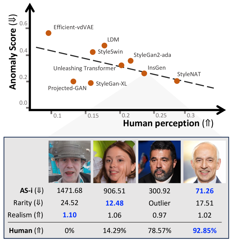
Figure 1: Proposed AS for evaluating generative models and AS-i for individual images. The graph on the top shows the proposed AS aligns well with the human perception of evaluating various generative models trained on the FFHQ dataset. On the bottom, several generated images are shown with our AS-i score, rarity score [18], realism score [30], and human evaluation. A value of the human evaluation indicates the proportion of participants who assess that the image is a natural image in our subjective test. The best score for each metric, indicating an image to be the most natural image is highlighted in blue. In terms of naturalness, AS-i shows the best alignment with human evaluation. On the other hand, the rarity score evaluates the second image, which is unnatural, as the most common in real images. The realism score also overestimates the leftmost image to be the most realistic.

The performance of generative models can be represented in various ways. Assessing how similar generated images are to real images (i.e., fidelity) is one of the most important and challenging aspects of evaluating the performance. An accurate approach is conducting subjective tests, where human subjects are asked to judge the naturalness of generated images, but this is resource-intensive and often even impractical. To efficiently evaluate generative models in various aspects, several objective metrics have been proposed [45, 21, 3, 44, 30, 18]. Most existing metrics involve comparing sample statistics between the sets of real and generated images after extracting features from pre-trained vision models. For instance, the Fréchet inception distance (FID) utilizes the Inception model [49] to extract Inception features and measures the 2-Wassertein distance of the Inception features between the real and generated datasets.

However, it is argued that such metrics are often misaligned with the human judgment on naturalness. In [31], it is shown that FID has a null space where the score is unaffected by the change of naturalness of generated images. Furthermore, [48] shows that the score often focuses on image parts unrelated to the naturalness. To sum up, existing metrics are subject to inconsistency to a certain extent in assessing the naturalness of generated images.

We argue that relying only on feature distances is insufficient to assess the naturalness of generated images. Consider a pair of real images having a certain distance in a representation space (i.e., feature space). We can modify one of the images (e.g., by adding noise) so that the modified one is at the same certain distance from the original image. In this case, while the feature distance between the two real images is the same as the distance between the chosen real image and its modified version, the modified image has significantly different contents in terms of naturalness. This also applies to generated images, having certain distances to real images may not be able to accurately represent whether the generated images are natural or not.

In order to address this limitation, in this paper, we propose two novel metrics: anomaly score (AS) for evaluating generative models and anomaly score for individual images (AS-i) for evaluating individual generated images. Instead of simply measuring distances between features, AS and AS-i capture the relationship between the input space and the representation space based on two new perspectives, complexity and vulnerability. We demonstrate that both metrics show significant correlations with the human-perceived naturalness of generated images (Fig. 1).

We define complexity as the amount of variations in the direction of feature changes with respect to linear input changes. A trained neural network model typically implements a non-linear function, and the degree of non-linearity (which we refer to as complexity) depends on the feature location in the representation space [28]. We observe that complexity tends to become larger for real images compared to unnatural generated images.

Vulnerability reflects how easily the extracted feature of an image is changed due to adversarial input changes. We apply the concept of adversarial attacks [17, 36, 10], which point out weaknesses of deep learning models and are also utilized for tasks capturing characteristics of images, such as out-of-distribution detection [34]. We observe that vulnerability tends to be smaller for real images compared to generated unnatural images.

Our contributions are summarized as follows.

1. We introduce complexity and vulnerability, to examine the characteristics of the representation space. Complexity measures how non-linear the representation space around an image is with respect to the linear input changes. And, vulnerability captures how easily an extracted feature is changed by adversarial input changes. We demonstrate that complexity and vulnerability of generated images are significantly different compared to those of real images.

2. We propose a novel metric called anomaly score (AS) to evaluate generative models in terms of naturalness based on complexity and vulnerability. AS is the difference of joint distributions of complexity and vulnerability between the sets of reference real images and generated images, which is quantified by 2D Kolmogorov-Smirnov (KS) statistics. Our method aligns better human judgment about the unnaturalness of generated images compared to the existing method.

3. We suggest the anomaly score for individual images (AS-i) to assess generated images individually. By conducting subjective tests, we demonstrate that AS-i outperforms existing methods for individual image evaluation.

2 Related works

2.1 Generative models

Generative models have garnered significant attention for their ability to generate realistic data samples. GANs [16, 25, 27, 47] leverage a game-theoretic approach, employing a generator and discriminator in a competitive setting. Variational autoencoders (VAEs) [19], on the other hand, model the distribution of the training data with a likelihood function, learning latent variable representations to generate data that closely matches the observed distribution. Recently, diffusion models [22, 13, 4] have emerged as a powerful approach in generating high-quality images and capturing complex data distributions.

2.2 Evaluation of generative models

Evaluation of generative models mostly involve comparing sample statistics between the generated data and the real target data. Existing metrics can be categorized into three groups based on the way of evaluation: summarizing overall performance of generative models in a single score [45, 21, 3], evaluating different aspects of performance (e.g., fidelity and diversity) of models separately [44, 30, 38], and assessing individual generated images [30, 18].

In the first category, FID [21] is one of the most widely used metrics, which measures how well a generative model can reproduce the target data distribution. It employs the trained Inception model [49] to extract features from the generated and the real images and measures the 2-Wasserstein distance between the two feature distributions. However, it often fails to model the density of the feature distributions [33] and to align with human perception [31].

For the second category, Precision and Recall [44, 30] measure fidelity and diversity of samples from generative models, respectively, by extending the classical precision and recall metrics for machine learning. They construct manifolds of the real samples and the generated samples in a certain representation space, then count the proportions of generated and real samples that belong to the real and generated manifolds, respectively. While such twofold metrics are effective for a diagnostic purpose, they are often vulnerable to outliers [38] and suffer from high computational costs for measuring pairwise distances between samples.

Few studies have addressed evaluation of individual samples [30, 18]. The realism score [30] examines the relationship between a generated image and the real manifold. Still, it is based on the manifold that is vulnerable to outliers, thus may become deviated from human evaluation (as will be shown in our experiments). The rarity score [18] focuses on how rare or uncommon a generated image is in order to consider the performance of generative models in terms of creativity. Thus, the rarity score does not provide accurate information about the naturalness of an image.

3 Analyzing representation space around generated images

In this section, we demonstrate that the representation space, which is the space of features extracted by pre-trained models for vision tasks, around generated images exhibits distinct properties in comparison to that around real images.

3.1 Complexity

Motivation. When an input of a trained model changes linearly, it is expected that its feature representation (i.e., output of the model before the softmax function) does not change linearly but instead exhibits curvature due to the non-linearity inherent in deep neural networks. In [28], it is observed that the regions around the features of training images in the representation space appear curved (i.e., complex) after training, i.e., a linear movement in the input space yields a curved trajectory in the representation space; on the other hand, the representation space near modified images with random noise is less complex. This suggests that the regions far from training images in the representation space are less complex when compared to those around the training images themselves. In a similar context, we hypothesize that the representation space around generated images is less complex than that surrounding reference real images.

Definition. To assess the complexity of the representation space around an image, we gradually add random noises to the image and quantify the angular variations in the corresponding feature movements. Let $\mathrm{x}$ and $\mathrm{N}$ denote an image and a Gaussian random noise vector having a unit length, respectively. $\mathrm{x}$ is corrupted gradually by $\epsilon\mathrm{N}$, i.e., the noised image at step $k$ is computed as $\mathrm{x}^{k}=\mathrm{x}^{0}+k\epsilon\mathrm{N}$, where $\epsilon$ is the parameter controlling the magnitude of noise and $\mathrm{x}^{0}=\mathrm{x}$. Then, we calculate the angle between the changes of the output feature within two successive steps (i.e., $k-1$ and $k$). For instance, when the features for $\mathrm{x}^{k-2}$, $\mathrm{x}^{k-1}$, and $\mathrm{x}^{k}$ are on a straight line, the angle is zero. We compute the complexity $\mathrm{C}(\cdot)$ by averaging the angles across the changes over multiple steps, which is formulated as follows.

$$\mathrm{C}(\mathrm{x})=\frac{1}{K}\sum_{k=1}^{K}\Big{(}\cos^{-1}{\frac{M(\mathrm{x}^{k-1})\cdot M(\mathrm{x}^{k})}{||M(\mathrm{x}^{k-1})||~{}||M(\mathrm{x}^{k})||}}\Big{)},$$ (1)

where $M(\cdot)$ indicates the model used for extracting features, which is referred to as feature model for simplicity, and $K$ represents the total number of steps of adding random noise. Note that the feature model can be chosen among various models trained for vision tasks, including models for ImageNet classification and models trained by self-supervised learning methods.

Experimental setup. We conduct an experiment to compare the complexity defined above for real images and generated images. We use six pre-trained models for the feature model ($M(\cdot)$): three supervised ImageNet classification models, ResNet50 [20], ViT-S [14], and ConvNeXt-tiny [35], and three self-supervised models, DINO [7], DINO-V2 [41], and CLIP [43]. We utilize three reference datasets, Cifar10 [29], ImageNet [11], and FFHQ [25]. We employ generated datasets produced by various generative models including GANs [40, 6, 52, 15, 23, 26, 27, 47, 2, 55, 46, 24, 54, 51, 8], VAEs [19, 32], a flow-based generative model [9], and diffusion models [22, 39, 4, 5, 13, 42, 12, 53, 50] from dgm-eval [48] and utilize 10000 generated images from each dataset. We set $\epsilon=0.01$ and $K=10$. More experimental details are described in the appendix.

		ViT	ConvNeXt	DINO-V2
Cifar10	Reference	0.1046	0.0986	0.0578
	Generated	0.1018	0.0975	0.0573
	$p$-value	$<$0.0001∗	$<$0.0001∗	$<$0.0005∗
ImageNet	Reference	0.0519	0.0485	0.0337
	Generated	0.0410	0.0287	0.0102
	$p$-value	$<$0.01∗	$<$0.0001∗	$<$0.0001∗
FFHQ	Reference	0.0643	0.0627	0.0311
	Generated	0.0638	0.0525	0.0302
	$p$-value	0.2495	$<$0.0001∗	$<$0.0001∗

Table 1: Complexity of various datasets. We compare the average value of complexity for various feature models, ViT-S [14], ConvNeXt-tiny [35], and DINO-V2 [41]. ‘Reference’ indicates the original dataset, such as Cifar10 [29], ImageNet [11], and FFHQ [25]. ‘Generated’ denotes the complexity obtained from datasets generated by PFGM++ [53], RQ Transformer [32], and InsGen [54] trained with the respective reference datasets. ‘$p$-value’ denotes the $p$-value of the one-tailed $t$-test under the null hypothesis that complexity of the generated dataset is equal to that of the reference dataset. The cases with statistical significance are marked with ‘$*$’.

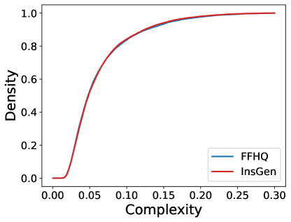
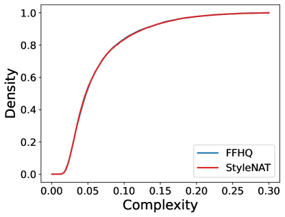
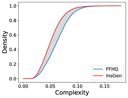
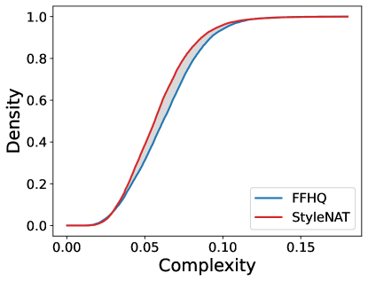
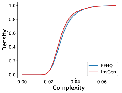
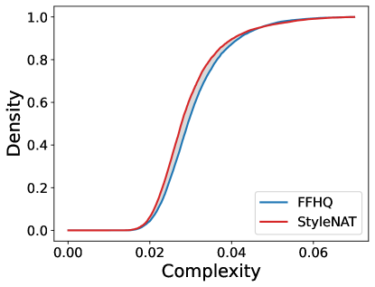
Figure 2: Distribution of complexity. The cumulative distribution function (CDF) of complexity is depicted for various feature models and generated datasets on FFHQ. Each row shows distributions for each feature model: ViT-S (top), ConvNeXt-tiny (mid), and DINO-V2 (bottom). Each column indicates a different type of generative model: InsGen [54] (left) and StyleNAT [51] (right). Note that InsGen is assessed as a low-performance model compared to StyleNAT by the human evaluation [48].

Results. Tab. 1 shows the average values of the complexity of the reference dataset and the generated dataset. Overall, the complexity of the generated images is smaller than that of the reference images, which is confirmed by statistical tests, indicating that as expected, generated images are located in less complex regions in the representation space than the reference (real) images. Fig. 4 presents the cumulative distribution function (CDF) of complexity for various feature models and datasets. In most cases, the distribution of the generated dataset differs from that of the reference dataset. Furthermore, the datasets generated by the InsGen model (left column), which generates relatively low-quality images, have more deviated distributions of complexity compared to the datasets generated by the StyleNAT model, which generates higher-quality images. The difference between the original dataset and the generated one is especially prominent in the case of using the ConvNeXt-tiny feature model.

3.2 Vulnerability

Motivation. We exploit the idea of adversarial attack [17, 36, 10] as another tool for examining the relationship between the input space and the representation space. In particular, we generate adversarial perturbations that cause large changes in the representation space with small changes in the input space. As a result, we observe that unnatural components (regions) of images tend to cause large changes. The left column of Fig. 3 shows examples of unnatural components of images, specifically the chin of the girl (upper panel) and the right side of the man (lower panel). For each image, we employ the SLIC algorithm [1] to divide the image into 20 super-pixels. Then, we randomly select 3 to 6 super-pixels among 20 super-pixels, add adversarial perturbations determined by PGD [36] to the selected super-pixels, and obtain the feature of the attacked image from a feature model. We repeat this process 20 times. We apply linear regression between the binary variables indicating whether each super-pixel is attacked and the amount of feature change, and the obtained coefficient of each variable is considered as the contribution of each super-pixel to the feature change (see the appendix for more details). The second to fourth columns of Fig. 3 show the contribution of each super-pixel to the feature changes for different feature models with the color coding. Across all models, unnatural super-pixels are consistently highlighted in red, i.e., the feature of the image is largely changed when we add adversarial perturbations to the unnatural super-pixels. Based on this result, we consider that examining the feature change of an image under adversarial attack can be an effective way to identify unnaturalness of the image.

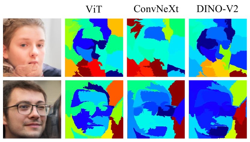
Figure 3: Image components causing large changes by adversarial attack. We partition images into super-pixels and assess their contribution to feature changes by the attack. Starting from the left: the original image, and the level of contributions on the changes in the feature extracted by ViT-S [14], ConvNeXt-tiny [35], and DINO-V2 [41], respectively. The red color denotes a high level of impact on the changes, while the blue color indicates a low level of influence on the changes.

		ViT	ConvNeXt	DINO-V2
Cifar10	Reference	24.56	14.57	29.41
	Generated	24.98	15.24	30.32
	$p$-value	$<$0.0001∗	$<$0.0001∗	$<$0.0001∗
ImageNet	Reference	11.73	8.69	8.06
	Generated	15.80	12.45	12.85
	$p$-value	$<$0.0001∗	$<$0.0001∗	$<$0.0001∗
FFHQ	Reference	18.30	14.57	12.90
	Generated	19.22	17.21	16.34
	$p$-value	$<$0.0001∗	$<$0.0001∗	$<$0.0001∗

Table 2: Vunerability of various datasets. We compare the average value of vulnerability for various feature models, ViT-S [14], ConvNeXt-tiny [35], and DINO-V2 [41]. ‘Reference’ indicates the original dataset, such as Cifar10 [29], ImageNet [11], and FFHQ [25]. ‘Generated’ denotes the vulnerability obtained from datasets generated by PFGM++ [53], RQ Transformer [32], and InsGen [54] trained with the respective reference datasets. ‘$p$-value’ denotes the $p$-value of the one-tailed $t$-test under the null hypothesis that vulnerability of the generated dataset is equal to that of the reference dataset. The cases with statistical significance are marked with ‘$*$’.

Definition. The PGD attack [36] is a widely used method for altering prediction results of a model through iterative perturbations applied to images. While the original PGD attack targeting classification models aims to maximize the cross-entropy loss, we maximize the $L_{2}$ loss between the features of the original and attacked images.

Starting from $\mathrm{x}^{0}=\mathrm{x}+\delta\mathrm{N}$, the image is iteratively perturbed as follows. Let $\mathrm{P}^{j}$ and $\mathrm{x}^{j}$ denote the adversarial perturbation and the attacked image at the $j$-th step of the attack, respectively. The modified PGD update rule is given by

$$\mathrm{\tilde{P}}^{j}=\nabla_{\mathrm{x}^{j}}{L_{2}(M(\mathrm{x}),M(\mathrm{x}^{j}))},$$ (2)

$$\mathrm{P}^{j}=\alpha~{}\mathrm{\tilde{P}}^{j}/||\mathrm{\tilde{P}}^{j}||,$$ (3)

$${\mathrm{x}}^{j+1}=\mathrm{Clip}_{0,255}(\mathrm{x}^{j}+\mathrm{P}^{j}),$$ (4)

where $\alpha$ is the attack size at each step, $M(\cdot)$ indicates the feature model, and $L_{2}(M(\mathrm{x}),M(\mathrm{x}^{j}))$ is the $L_{2}$ loss between the features of the original and modified inputs. $\mathrm{Clip}_{0,255}(\cdot)$ is a clipping function that limits values to the range between 0 and 255.

Then, we define vulnerability of image $\mathrm{x}$, $\mathrm{V}(\mathrm{x})$, as follows:

$$\mathrm{V}(\mathrm{x})=dist(M(\mathrm{x}),M(\mathrm{x}^{J})),$$ (5)

where $J$ is the total number of steps of the attack and $dist(A,B)$ indicates the $L_{2}$ distance between two vectors $A$ and $B$.

Experimental setup. We conduct an experiment to examine the validity of the vulnerability for evaluating unnaturalness of generated images. We set $\alpha=0.01$, $\delta=10^{-6}$, and $J=10$ in this experiment, while keeping all other settings, such as feature models and generative models, the same as those used in Sec. 3.1.

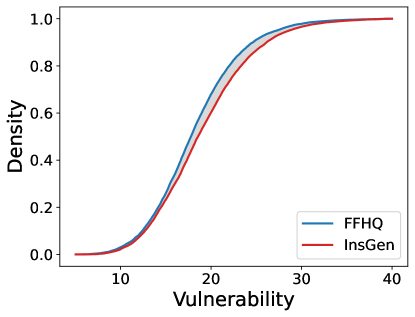
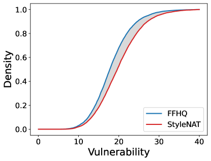
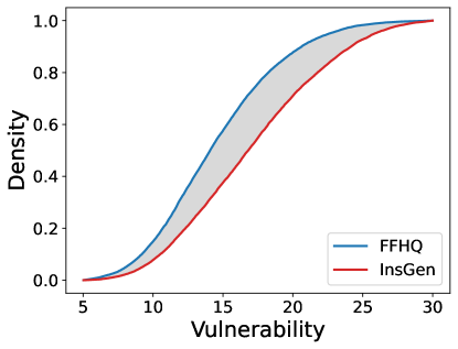
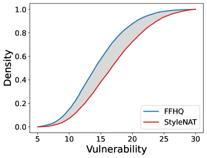
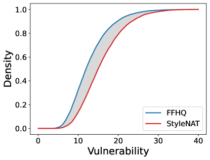
Figure 4: Distribution of vulnerability. The cumulative distribution function (CDF) of vulnerability is depicted for various feature models and generated datasets on FFHQ. Each row shows distributions for each feature model: ViT-S (top), ConvNeXt-tiny (mid), and DINO-V2 (bottom). Each column indicates a different type of generative model: InsGen [54] (left) and StyleNAT [51] (right). Note that InsGen is assessed as a low-performance model compared to StyleNAT by the human evaluation [48].

Results. Tab. 2 shows the average vulnerability of images from various datasets on ViT-S, ConvNeXt-tiny, and DINO-V2 as feature models. Further results for other models are shown in the appendix. It can be seen that the vulnerability of generated images is larger than that of reference images. Fig. 4 also shows the significant disparity in the vulnerability distribution between real and generated images. Furthermore, the high-quality generated dataset by the StyleNAT model has a more similar distribution to that of the reference dataset compared to the relatively low-quality generated dataset by the InsGen model in most cases, which is consistent with the results observed in the comparison of complexity.

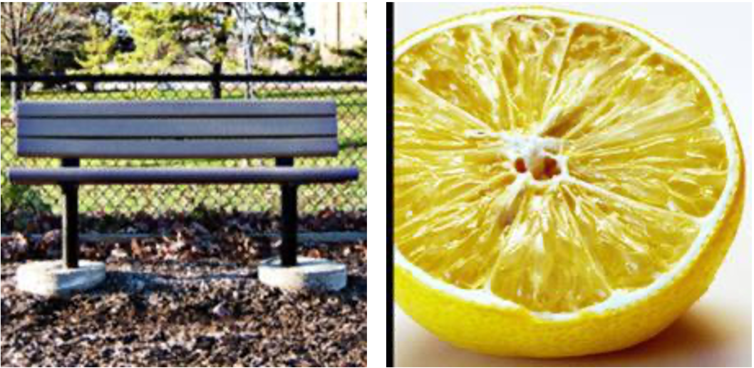
(a) Low-MVT level

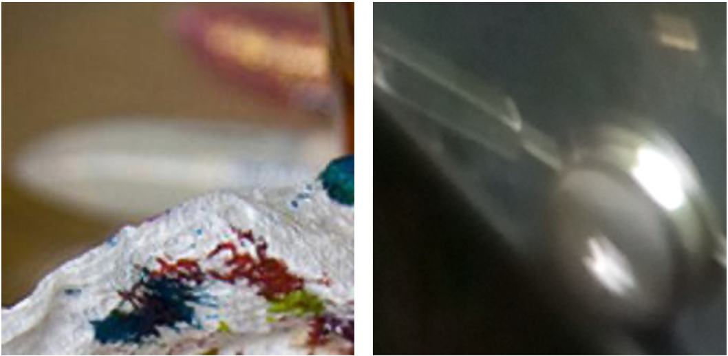
(b) High-MVT level

Figure 5: Examples of the MVT dataset. Images having low MVT levels are clear for people to recognize. On the other hand, a high MVT level means that people need a long time to recognize the image contents due to weak naturalness.

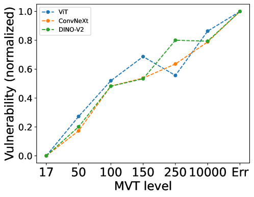
Figure 6: Vulnerability vs. MVT levels. The average value of vulnerability of images having each MVT level. Note that the value of vulnerability is normalized by the maximum and the minimum values in each feature model.

Vulnerability and naturalness. We further demonstrate the relationship between vulnerability and naturalness. We employ the MVT dataset [37], which contains information on the difficulty for humans to recognize objects in each image by measuring the minimum viewing time required for recognition. In the dataset, the viewing time is separated into several levels called MVT levels (i.e., 17 ms, 50 ms, 100 ms, 150 ms, 250 ms, and 10,000 ms). Each MVT level means the time within which over 50% of participants can correctly classify an object. It is linked to the level of unnaturalness of the images. In other words, when an image contains clear content (Fig. 5(a)), humans swiftly identify the depicted object under 50 ms. Conversely, an image with unnatural components (Fig. 5(b)) poses a challenge for human recognition, requiring over 10,000 ms.

Fig. 6 shows the vulnerability with respect to the MVT level. Here, “Err” indicates that over 50% of participants misclassify an image given sufficient time. The MVT level is highly correlated with the vulnerability on all feature models, i.e., low naturalness is related to high vulnerability.

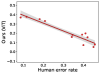
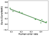
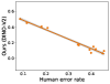
(a) Cifar10

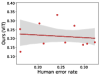
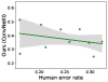
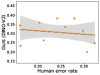
(b) ImageNet

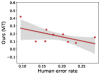
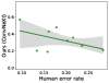
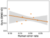
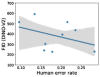
(c) FFHQ

Figure 7: Overall results of evaluating generative models on various datasets. Each dot represents a distinct dataset generated by a generative model. A high human error rate indicates a high-quality dataset, while a high AS score means a low-quality dataset. The first three columns show AS with different feature models: DINO-V2, ConvNeXt-tiny, and ViT-S, respectively. The last column is the result of FID [21] with the DINO-V2 model.

4 Evaluating generative models

In the previous section, we explored the distinct properties in the representation space around generated images in comparison to those of real images. The representation space around generated images is more complex (complexity) and contains a certain path that is vulnerable to adversarial changes (vulnerability). Thus, we propose a novel metric for evaluating generative models by capturing anomalies based on both complexity and vulnerability, called anomaly score.

4.1 Anomaly score for generative models

We define anomaly score (AS) for evaluating generative models as the difference of the bivariate distributions of complexity and vulnerability between the reference and generated datasets. We denote the set of anomaly vectors for the dataset $\mathrm{X}$ as $\textrm{A}(\mathrm{X})=\{[\textrm{C}(\mathrm{x}),\textrm{V}(\mathrm{x})]\}_{\mathrm{x}\in\mathrm{X}}$.

To compare the distributions of the generated dataset and the reference dataset, we employ the Kolmogorov-Smirnov (KS) statistic that measures a non-parametric statistical difference between two distributions. Our anomaly score, AS, utilizing the 2D KS statistic, is defined as

$$\textrm{AS}=\big{|}\textrm{CDF}(\textrm{A}(\mathrm{X}^{real}))-\textrm{CDF}(\textrm{A}(\mathrm{X}^{generated}))\big{|},$$ (6)

where $\mathrm{X}^{real}$ is the reference dataset for the generated dataset, $\mathrm{X}^{generated}$, and $\textrm{CDF}(\cdot)$ is the cumulative distribution function of input vectors. We employ 2D KS statistics by referencing github.com/syrte/ndtest. AS has the minimum value of 0 when the two distributions are identical and the maximum value of 1 when the two distributions are significantly different, i.e., their CDFs are completely non-overlapped.

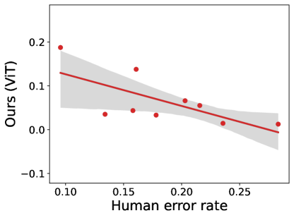
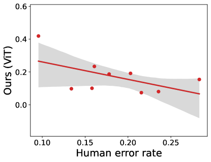
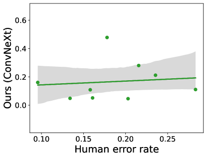
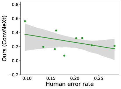
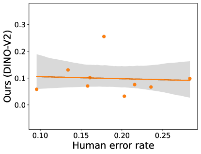
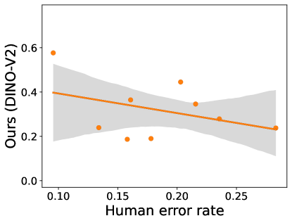
Figure 8: Anomaly score using one measure. Each dot represents a distinct generated dataset produced by a generative model for the FFHQ dataset. A high human error rate means a high-quality dataset, while a high AS implies a low-quality dataset. Each row corresponds to a different feature model, and each column represents the results obtained by using the distribution of complexity (left) or vulnerability (right).

4.2 Experiments

Setup. To evaluate the effectiveness of our metric, we examine whether our scores align with the subjective scores reported in [48]. In this subjective test, human viewers responded whether a given image appeared fake (generated) or real. Note that a high human error rate for a generated dataset indicates that many viewers cannot identify the images as fake ones, implying that the images in the dataset have high quality and are realistic. We use the same generated datasets in [48] and measure AS with various feature models.

Results. Fig. 7 shows the comprehensive performance of various generative models evaluated by our method with ViT-S, ConvNeXt-tiny, and DINO-V2 as the feature models. For comparison, the conventional FID with DINO-V2 as the feature model is also evaluated. Additional results for other models are presented in the appendix. Our method outperforms FID (the last column) on the FFHQ dataset. Our method has a relatively high correlation (-0.56 pearson correlation coefficient (PCC)) with human perception, while FID has a lower correlation (-0.38 PCC). We can observe that AS with DINO-V2 (-0.98 PCC), ConvNeXt-tiny (-0.30 PCC), and ViT-S (-0.56 PCC) are well aligned with the human error rate on Cifar10, ImageNet, and FFHQ, respectively.

1D test. In our method, we utilize both complexity and vulnerability of the images. We conduct a comparative analysis using only one of the two in the anomaly vector, where the 1D KS statistic is used instead of the 2D KS statistic. Fig. 8 presents the results on the FFHQ dataset. Complexity performs well with ViT-S (-0.69 PCC) but not with ConvNeXt-tiny and DINO-V2 (0.11 and -0.07 PCCs, respectively). Vulnerability shows decent performance over all feature models (-0.55, -0.40, and -0.39 PCCs, respectively), but is outperformed by our method employing both complexity and vulnerability (-0.56, -0.48, and -0.42 PCCs, respectively). These results demonstrate the benefit of employing both complexity and vulnerability in our AS in terms of both performance and consistency.

5 Evaluating individual generated images

In this section, we propose a method for evaluating generated images individually based on complexity and vulnerability defined in Sec. 3.

5.1 Anomaly score for individual generated images

We adopt a simple and effective formula to capture the properties of complexity and vulnerability of an image in a single score. The proposed anomaly score for individual images (AS-i) is defined as follows:

$$\textrm{AS-i}(\mathrm{x})=\frac{\textrm{V}(\mathrm{x})}{\textrm{C}(\mathrm{x})},$$ (7)

where $\mathrm{x}$ represents an individual generated image. When the image is natural, complexity around the image increases (large $\textrm{C}(\mathrm{x})$) and vulnerability of the image decreases (small $\textrm{V}(\mathrm{x})$), hence AS-i becomes small. On the other hand, when the image is unnatural, AS-i becomes large.

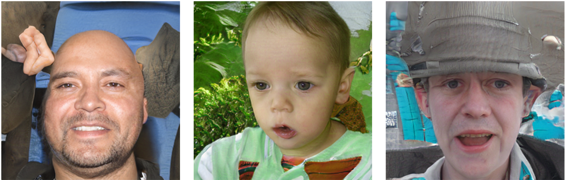
(a) Examples having high AS-i

(b) Examples having medium AS-i (around 600)

(c) Examples having low AS-i

Figure 9: Examples having various levels of AS-i.

5.2 Subjective test

Experimental settings. To verify that AS-i captures human judgement well in terms of the naturalness of images, we conduct a subjective test using the images generated by InsGen [54]. We set five levels of AS-i (highest in the dataset, 900, 600, 300, and lowest in the dataset) using the ConvNeXt-tiny feature model. The highest level of AS-i ranges from 1434 to 1746 with an average of 1561 and the lowest level ranges from 53 to 80 with an average of 71. Then, for each level, we form an image subset by sampling 20 images having AS-i close to the level. Fig. 9 shows several examples of images that belong to the highest, medium (600), and the lowest levels. 14 participants are asked to judge if each image appears natural. We consider an image to be natural if over 50% of the participants respond that the image is natural as in [37]. Then, we obtain the proportion of the number of images that are identified as natural in each subset.

AS-i	Human	Rarity [18]	Realism [30]
Low	0.75	21.82	1.039
300	0.50	18.47	1.036
600	0.40	21.51	1.030
900	0.30	21.54	1.032
high	0.25	20.16	1.010

Table 3: Evaluation of AS-i. For each level of AS-i, the proportion of images judged as natural by participants, the average rarity score, and the average realism score are shown.

Results and comparison. Tab. 3 presents the results of the subjective test. It is observed that as AS-i level increases, less images in a subset are judged as natural in a consistent manner. On the other hand, the average rarity score [18] and realism score [30] are not aligned well with human perception. The PCCs for AS-i, rarity score, and realism score are -0.88, -0.49, and 0.63, respectively.

6 Conclusion

We have proposed new metrics, AS and AS-i, for evaluation of generative models and individual generated images, respectively. Both are based on complexity and vulnerability, which examine the representation space around the images. Complexity captures the curvedness of the representation space, while vulnerability tests the changes in the representation space under adversarial attack. We demonstrated that the proposed metrics accord well with human judgments and outperform existing metrics.

Supplementary Material

In this supplementary material, we include additional materials, which are not contained in the main paper because of the page limit, such as an explanation of the employed generative models and details of the linear regression on vulnerability. We also provide additional experimental results on various feature models and examples of generated images that are used for the subjective test.

Appendix A Employed generative models

We utilize various generated datasets from https://github.com/layer6ai-labs/dgm-eval [48], which are listed below with respect to the target image dataset.

• Cifar10 [29]: ACGAN [40], BigGAN [6], IDDPM [39], LoGAN [52], LSGM [50], MHGAN [15], PFGM++ [53], ReacGAN [23], ResFlow [9], StyleGAN-XL [47], StyleGAN2-ada [27], WGAN [2]

• ImageNet [11]: ADM [13], BigGAN [6], DiT-XL-2 [42], GigaGAN [24], LDM [4], Mask-GIT [8], RQ-Transformer [32], StyleGAN-XL [47], ADMG [12], ADMG-ADMU [12]

• FFHQ [25]: Efficient-vdVAE [19], InsGen [54], LDM [4], StyleGAN-XL [47], StyleGAN2-ada [27], StyleNAT [51], StyleSwin [55], Unleashing-transformers [5], Projected GAN [46]

Appendix B Linear regression on vulnerability

In Sec 3.2, we explore the motivation of vulnerability by calculating the contributions of super-pixels of images to the changes caused by adversarial attacks. We randomly select 3 to 6 super-pixels, add adversarial perturbations into them, and obtain the changes in the features due to the perturbations. We repeat this process 20 times. Then, we apply linear regression between the feature change and the set of binary variables indicating whether each super-pixel is attacked or not. The linear regression is described as: $\textrm{Y}=\textrm{V}\textrm{W}+b,$ where Y is a 20 (# of trials)$\times$1 vector of the feature change, V is a 20 (# of trials)$\times$20 (# of super-pixels) matrix of variables that indicate whether each super-pixel is selected or not on each trial, W is a 20 (# of super-pixels)$\times$1 vector of the linear regression coefficient, and $b$ is a 20 (# of trials)$\times$1 vector of bias. We consider the linear regression coefficient W as the contribution of each super-pixel to the feature changes, i.e., vulnerability. If the coefficient is large, the corresponding super-pixel greatly contributes to the vulnerability. On the other hand, if the coefficient is small, the corresponding super-pixel contributes less to the vulnerability.

Appendix C Results on various feature models

Complexity		ResNet50	CLIP	DINO
Cifar10	Reference	0.1900	1.9246	0.0647
	Generated	0.1921	1.9234	0.0626
	$p$-value	-	0.0853	$<$0.0001∗
ImageNet	Reference	0.1170	1.9543	0.0326
	Generated	0.1190	1.9366	0.0331
	$p$-value	-	$<$0.0001∗	-
FFHQ	Reference	0.1273	1.9899	0.0424
	Generated	0.1233	1.9893	0.0352
	$p$-value	$<$0.0001∗	0.1489	$<$0.0001∗

Vulnerability		ResNet50	CLIP	DINO
Cifar10	Reference	44.59	6.67	37.40
	Generated	44.31	6.69	35.56
	$p$-value	-	$<0.05$∗	-
ImageNet	Reference	32.18	4.54	9.27
	Generated	35.58	5.12	11.98
	$p$-value	$<$0.0001∗	$<$0.0001∗	$<$0.0001∗
FFHQ	Reference	30.22	4.52	13.9
	Generated	30.85	4.39	12.57
	$p$-value	$<$0.0001∗	-	-

Table C.1: Complexity and vulnerability of various datasets. We compare the average value of vulnerability for various feature models, ResNet50 [20], CLIP [43], and DINO [7]. ‘Reference’ indicates the original dataset, such as Cifar10 [29], ImageNet [11], and FFHQ [25]. ‘Generated’ denotes datasets generated by PFGM++ [53], RQ Transformer [32], and InsGen [54] trained with the respective reference datasets. ‘$p$-value’ denotes the $p$-value of the one-tailed $t$-test under the null hypothesis that complexity or vulnerability of the generated dataset is equal to that of the reference dataset. The cases with statistical significance are marked with ‘$*$’. ‘-’ means that the expectation is not met, i.e., complexity (vulnerability) of the generated dataset is larger (smaller) than that of the reference dataset.

We use six feature models, ResNet50 [20], ViT-S [14], ConvNeXt-tiny [35], CLIP [43], DINO [7], and DINO-V2 [41]. Here, we present the experimental results on ResNet50, CLIP, and DINO, which are not included in the main paper.

C.1 Complexity and vulnerability

Tab. C.1 indicates the average values of complexity and vulnerability of the reference datasets and generated datasets when we use ResNet50, CLIP, and DINO as the feature model. In most cases, complexity of the generated datasets is smaller than that of the reference datasets. Vulnerability of the generated datasets is larger than that of the reference datasets except for a few cases. These results are generally consistent with the results in the main paper (Tab. 1 and Tab. 2). However, in some cases using ResNet50 and DINO, the results are not aligned with our assumption, implying that they are less preferable as the feature model of our method.

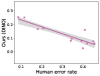
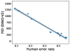
(a) Cifar10

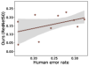
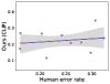
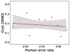
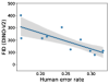
(b) ImageNet

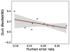
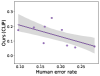
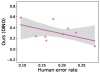
(c) FFHQ

Figure C.1: Overall results of evaluating generative models on various datasets. Each dot represents a distinct dataset generated by a generative model. A high human error rate indicates a high-quality dataset, while a high AS score means a low-quality dataset. The first three columns show AS with different feature models: ResNet50, CLIP, and DINO, respectively. The last column is the result of FID [21] with the DINO-V2 model.

C.2 Anomaly score

Fig. C.1 shows the performance of various generative models by the proposed anomaly score with ResNet50, CLIP, and DINO as feature models and FID with DINO-V2. In the case of Cifar10 and FFHQ, the anomaly score evaluates generated datasets well with high correlations with human perception (-0.72, -0.36, and -0.89 pearson correlation coefficients (PCCs) on Cifar10, and -0.47, -0.60, and -0.51 PCCs on FFHQ, respectively). On the other hand, the anomaly score with ResNet50, CLIP, and DINO shows low correlations when we evaluate the generated datasets for ImageNet (0.45, 0.17, and -0.16 PCCs, respectively). Due to the weak alignment between the characteristics of the representation space of ResNet50, CLIP, and DINO and our assumptions (Sec. C.1), the performance of the anomaly score using them is lower than that using ViT-S, ConvNeXt-tiny, and DINO-V2.

Appendix D Images for subjective test

In Sec. 5 of the main paper, we evaluate our anomaly score for individual images, AS-i, by conducting the subjective test with 20 images for each AS-i level. Fig. D.1 shows example images according to each AS-i level. If an image has a low AS-i level, the image looks natural and clear, like real images. Images with higher AS-i levels contain more unnatural components, such as abnormal patterns in faces and backgrounds. Fig. D.1 shows that the severity of the unnatural pattern in the image increases as the AS-i level increases.

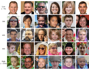
Figure D.1: Examples having various levels of AS-i.

References

- Achanta et al. [2012] Radhakrishna Achanta, Appu Shaji, Kevin Smith, Aurelien Lucchi, Pascal Fua, and Sabine Süsstrunk. SLIC superpixels compared to state-of-the-art superpixel methods. IEEE TPAMI, 34(11):2274–2282, 2012.
- Arjovsky et al. [2017] Martin Arjovsky, Soumith Chintala, and Léon Bottou. Wasserstein generative adversarial networks. In ICML, pages 214–223, 2017.
- Bińkowski et al. [2018] Mikołaj Bińkowski, Danica J. Sutherland, Michael Arbel, and Arthur Gretton. Demystifying MMD GANs. In ICLR, 2018.
- Blattmann et al. [2023] Andreas Blattmann, Robin Rombach, Huan Ling, Tim Dockhorn, Seung Wook Kim, Sanja Fidler, and Karsten Kreis. Align your latents: High-resolution video synthesis with latent diffusion models. In CVPR, pages 22563–22575, 2023.
- Bond-Taylor et al. [2022] Sam Bond-Taylor, Peter Hessey, Hiroshi Sasaki, Toby P Breckon, and Chris G Willcocks. Unleashing transformers: Parallel token prediction with discrete absorbing diffusion for fast high-resolution image generation from vector-quantized codes. In ECCV, pages 170–188. Springer, 2022.
- Brock et al. [2018] Andrew Brock, Jeff Donahue, and Karen Simonyan. Large scale gan training for high fidelity natural image synthesis. In ICLR, 2018.
- Caron et al. [2021] Mathilde Caron, Hugo Touvron, Ishan Misra, Hervé Jégou, Julien Mairal, Piotr Bojanowski, and Armand Joulin. Emerging properties in self-supervised vision transformers. In ICCV, pages 9650–9660, 2021.
- Chang et al. [2022] Huiwen Chang, Han Zhang, Lu Jiang, Ce Liu, and William T Freeman. Maskgit: Masked generative image transformer. In CVPR, pages 11315–11325, 2022.
- Chen et al. [2019] Ricky TQ Chen, Jens Behrmann, David K Duvenaud, and Jörn-Henrik Jacobsen. Residual flows for invertible generative modeling. NeurIPS, 32, 2019.
- Croce and Hein [2020] Francesco Croce and Matthias Hein. Reliable evaluation of adversarial robustness with an ensemble of diverse parameter-free attacks. In ICML, 2020.
- Deng et al. [2009] Jia Deng, Wei Dong, Richard Socher, Li-Jia Li, Kai Li, and Li Fei-Fei. ImageNet: A large-scale hierarchical image database. In CVPR, pages 248–255, 2009.
- Dhariwal and Nichol [2021a] Prafulla Dhariwal and Alexander Nichol. Diffusion models beat gans on image synthesis. NeurIPS, 34:8780–8794, 2021a.
- Dhariwal and Nichol [2021b] Prafulla Dhariwal and Alexander Quinn Nichol. Diffusion models beat GANs on image synthesis. In NeurIPS, 2021b.
- Dosovitskiy et al. [2021] Alexey Dosovitskiy, Lucas Beyer, Alexander Kolesnikov, Dirk Weissenborn, Xiaohua Zhai, Thomas Unterthiner, Mostafa Dehghani, Matthias Minderer, Georg Heigold, Sylvain Gelly, Jakob Uszkoreit, and Neil Houlsby. An image is worth 16x16 words: Transformers for image recognition at scale. In ICLR, 2021.
- Du et al. [2020] Kangning Du, Huaqiang Zhou, Lin Cao, Yanan Guo, and Tao Wang. Mhgan: Multi-hierarchies generative adversarial network for high-quality face sketch synthesis. IEEE Access, 8:212995–213011, 2020.
- Goodfellow et al. [2014] Ian J. Goodfellow, Jean Pouget-Abadie, Mehdi Mirza, Bing Xu, David Warde-Farley, Sherjil Ozair, Aaron Courville, and Yoshua Bengio. Generative adversarial nets. In NeurIPS, pages 2672–2680, 2014.
- Goodfellow et al. [2015] Ian J Goodfellow, Jonathon Shlens, and Christian Szegedy. Explaining and harnessing adversarial examples. In ICLR, 2015.
- Han et al. [2023] Jiyeon Han, Hwanil Choi, Yunjey Choi, Junho Kim, Jung-Woo Ha, and Jaesik Choi. Rarity score : A new metric to evaluate the uncommonness of synthesized images. In ICLR, 2023.
- Hazami et al. [2022] Louay Hazami, Rayhane Mama, and Ragavan Thurairatnam. Efficient-VDVAE: Less is more. arXiv preprint arXiv:2203.13751, 2022.
- He et al. [2016] Kaiming He, Xiangyu Zhang, Shaoqing Ren, and Jian Sun. Deep residual learning for image recognition. In CVPR, pages 770–778, 2016.
- Heusel et al. [2017] Martin Heusel, Hubert Ramsauer, Thomas Unterthiner, Bernhard Nessler, and Sepp Hochreiter. GANs trained by a two time-scale update rule converge to a local Nash equilibrium. In NeurIPS, pages 6629–6640, 2017.
- Ho et al. [2020] Jonathan Ho, Ajay Jain, and Pieter Abbeel. Denoising diffusion probabilistic models. NeurIPS, 33:6840–6851, 2020.
- Kang et al. [2021] Minguk Kang, Woohyeon Shim, Minsu Cho, and Jaesik Park. Rebooting acgan: Auxiliary classifier gans with stable training. NeurIPS, 34:23505–23518, 2021.
- Kang et al. [2023] Minguk Kang, Jun-Yan Zhu, Richard Zhang, Jaesik Park, Eli Shechtman, Sylvain Paris, and Taesung Park. Scaling up gans for text-to-image synthesis. In CVPR, pages 10124–10134, 2023.
- Karras et al. [2019a] Tero Karras, Samuli Laine, and Timo Aila. A style-based generator architecture for generative adversarial networks. In CVPR, pages 4401–4410, 2019a.
- Karras et al. [2019b] Tero Karras, Samuli Laine, and Timo Aila. A style-based generator architecture for generative adversarial networks. In CVPR, 2019b.
- Karras et al. [2020] Tero Karras, Samuli Laine, Miika Aittala, Janne Hellsten, Jaakko Lehtinen, and Timo Aila. Analyzing and improving the image quality of StyleGAN. In CVPR, 2020.
- Kim et al. [2022] Juyeop Kim, Junha Park, Songkuk Kim, and Jong-Seok Lee. Curved representation space of vision transformers. arXiv preprint arXiv:2210.05742, 2022.
- Krizhevsky et al. [2009] Alex Krizhevsky et al. Learning multiple layers of features from tiny images. Technical report, 2009.
- Kynkäänniemi et al. [2019] Tuomas Kynkäänniemi, Tero Karras, Samuli Laine, Jaakko Lehtinen, and Timo Aila. Improved precision and recall metric for assessing generative models. In NeurIPS, 2019.
- Kynkäänniemi et al. [2023] Tuomas Kynkäänniemi, Tero Karras, Miika Aittala, Timo Aila, and Jaakko Lehtinen. The role of ImageNet classes in fréchet Inception distance. In ICLR, 2023.
- Lee et al. [2022] Doyup Lee, Chiheon Kim, Saehoon Kim, Minsu Cho, and Wook-Shin Han. Autoregressive image generation using residual quantization. In CVPR, pages 11523–11532, 2022.
- Lee and Lee [2022] Junghyuk Lee and Jong-Seok Lee. TREND: Truncated generalized normal density estimation of Inception embeddings for GAN evaluation. In ECCV, pages 87–103, 2022.
- Liang et al. [2018] Shiyu Liang, Yixuan Li, and Rayadurgam Srikant. Enhancing the reliability of out-of-distribution image detection in neural networks. In ICLR, 2018.
- Liu et al. [2022] Zhuang Liu, Hanzi Mao, Chao-Yuan Wu, Christoph Feichtenhofer, Trevor Darrell, and Saining Xie. A convnet for the 2020s. In CVPR, pages 11976–11986, 2022.
- Madry et al. [2018] Aleksander Madry, Aleksandar Makelov, Ludwig Schmidt, Dimitris Tsipras, and Adrian Vladu. Towards deep learning models resistant to adversarial attacks. In ICLR, 2018.
- Mayo et al. [2023] David Mayo, Jesse Cummings, Xinyu Lin, Dan Gutfreund, Boris Katz, and Andrei Barbu. How hard are computer vision datasets? calibrating dataset difficulty to viewing time. In NIPS Datasets and Benchmarks Track, 2023.
- Naeem et al. [2020] Muhammad Ferjad Naeem, Seong Joon Oh, Youngjung Uh, Yunjey Choi, and Jaejun Yoo. Reliable fidelity and diversity metrics for generative models. In NeurIPS, pages 7176–7185, 2020.
- Nichol and Dhariwal [2021] Alexander Quinn Nichol and Prafulla Dhariwal. Improved denoising diffusion probabilistic models. In ICML, pages 8162–8171, 2021.
- Odena et al. [2017] Augustus Odena, Christopher Olah, and Jonathon Shlens. Conditional image synthesis with auxiliary classifier gans. In ICML, pages 2642–2651, 2017.
- Oquab et al. [2023] Maxime Oquab, Timothée Darcet, Théo Moutakanni, Huy Vo, Marc Szafraniec, Vasil Khalidov, Pierre Fernandez, Daniel Haziza, Francisco Massa, Alaaeldin El-Nouby, et al. Dinov2: Learning robust visual features without supervision. arXiv preprint arXiv:2304.07193, 2023.
- Peebles and Xie [2023] William Peebles and Saining Xie. Scalable diffusion models with transformers. In ICCV, pages 4195–4205, 2023.
- Radford et al. [2021] Alec Radford, Jong Wook Kim, Chris Hallacy, Aditya Ramesh, Gabriel Goh, Sandhini Agarwal, Girish Sastry, Amanda Askell, Pamela Mishkin, Jack Clark, et al. Learning transferable visual models from natural language supervision. In ICML, pages 8748–8763. PMLR, 2021.
- Sajjadi et al. [2018] Mehdi S. M. Sajjadi, Olivier Bachem, Mario Lucic, Olivier Bousquet, and Sylvain Gelly. Assessing generative models via precision and recall. In NeurIPS, pages 5234–5243, 2018.
- Salimans et al. [2016] Tim Salimans, Ian Goodfellow, Wojciech Zaremba, Vicki Cheung, Alec Radford, Xi Chen, and Xi Chen. Improved techniques for training GANs. In NeurIPS, pages 2234–2242, 2016.
- Sauer et al. [2021] Axel Sauer, Kashyap Chitta, Jens Müller, and Andreas Geiger. Projected gans converge faster. NeurIPS, 34:17480–17492, 2021.
- Sauer et al. [2022] Axel Sauer, Katja Schwarz, and Andreas Geiger. StyleGAN-XL: Scaling StyleGAN to large diverse datasets. In Special Interest Group on Computer Graphics and Interactive Techniques Conference Proceedings, pages 1–10, 2022.
- Stein et al. [2023] George Stein, Jesse C. Cresswell, Rasa Hosseinzadeh, Yi Sui, Brendan Leigh Ross, Valentin Villecroze, Zhaoyan Liu, Anthony L. Caterini, J. Eric T. Taylor, and Gabriel Loaiza-Ganem. Exposing flaws of generative model evaluation metrics and their unfair treatment of diffusion models. arXiv preprint arXiv:2306.04675, 2023.
- Szegedy et al. [2016] Christian Szegedy, Vincent Vanhoucke, Sergey Ioffe, Jon Shlens, and Zbigniew Wojna. Rethinking the Inception architecture for computer vision. In CVPR, pages 2818–2826, 2016.
- Vahdat et al. [2021] Arash Vahdat, Karsten Kreis, and Jan Kautz. Score-based generative modeling in latent space. NeurIPS, 34:11287–11302, 2021.
- Walton et al. [2022] Steven Walton, Ali Hassani, Xingqian Xu, Zhangyang Wang, and Humphrey Shi. StyleNAT: Giving each head a new perspective. arXiv preprint arXiv:2211.05770, 2022.
- Wu et al. [2019] Yan Wu, Jeff Donahue, David Balduzzi, Karen Simonyan, and Timothy Lillicrap. Logan: Latent optimisation for generative adversarial networks. arXiv preprint arXiv:1912.00953, 2019.
- Xu et al. [2023] Yilun Xu, Ziming Liu, Yonglong Tian, Shangyuan Tong, Max Tegmark, and Tommi Jaakkola. PFGM++: Unlocking the potential of physics-inspired generative models. In ICML, 2023.
- Yang et al. [2021] Ceyuan Yang, Yujun Shen, Yinghao Xu, and Bolei Zhou. Data-efficient instance generation from instance discrimination. NeurIPS, 34:9378–9390, 2021.
- Zhang et al. [2022] Bowen Zhang, Shuyang Gu, Bo Zhang, Jianmin Bao, Dong Chen, Fang Wen, Yong Wang, and Baining Guo. Styleswin: Transformer-based gan for high-resolution image generation. In CVPR, pages 11304–11314, 2022.