Skein valued cluster transformation in
enumerative geometry of Legendrian mutation

Abstract.

Under certain hypotheses, we show that Legendrian surfaces related by disk surgery will have q-deformed augmentation spaces that are related by q-deformed cluster transformation. The proof is geometric, via considerations of moduli of holomorphic curves. In fact, our results naturally give a more general HOMFLYPT ‘skein-valued cluster transformation’, of which the q-cluster transformation is the U(1) specialization.

We apply our methods to the Legendrians associated to cubic planar graphs, where mutation of graphs lifts to Legendrian disk surgery. We show that their skein-valued mirrors transform by skein-valued cluster transformation, and give a formula for the skein-valued curve counts on their fillings.

1. Introduction

Cluster transformations are certain rational isomorphisms of Poisson tori with remarkable properties, found in nature in various settings such as combinatorial representation theory, Teichmüller theory, and symplectic geometry. We are concerned with this last connection, which appears in the context of homological mirror symmetry [25].

A particularly simple situation is the following. Consider a Weinstein symplectic 4-manifold $X$, and the moduli $\mathcal{M}(X)$ of pseudoperfect objects in the wrapped Fukaya category of $X$. Let $\Lambda\subset X$ be an exact Lagrangian. The moduli space of rank one brane structures on $\Lambda$ is the torus $\mathcal{M}_{1}(\Lambda)\cong H^{1}(\Lambda,\mathbb{C}^{*})$; it carries a symplectic structure induced from the Poincaré pairing on $\Lambda$. There is, essentially by definition, an open embedding $\mathcal{M}_{1}(\Lambda)\hookrightarrow\mathcal{M}(X)$. In particular, if $\Lambda,\Lambda^{\prime}$ are exact Lagrangians and $\mathcal{M}_{1}(\Lambda)\cap\mathcal{M}_{1}(\Lambda^{\prime})\neq\emptyset$, the intersection defines a rational isomorphism of Poisson tori. When $\Lambda$ and $\Lambda^{\prime}$ are related by Lagrangian disk surgery, the isomorphism can be identified with the simplest cluster transformation (see e.g. [3, 34, 28]). This (4d, exact) setting already contains many interesting cluster structures previously constructed combinatorially, in particular those associated to bicolored graphs on surfaces [35].

The theory of cluster transformations admits a q-deformation, from the Poisson tori to the corresponding quantum tori. It is natural to ask for a q-deformation of the above relationship between symplectic geometry and cluster transformations. Motivated by some reasoning from string theory, such a conjectural relation was proposed for one class of examples (cubic planar graph Legendrians) in the work of Schrader, Shen, and Zaslow [32]. The purpose of the present article is to describe a general setting for such a relationship, and its further lift to ‘skein-valued cluster transformations’.

1.1. Why we may expect to find skein valued cluster transformations

We move up in dimension. Let $W$ be a 6d Weinstein symplectic Calabi-Yau manifold, whose ideal contact boundary $\partial_{\infty}W$ contains the above $X$ as a Liouville hypersurface. (All the examples we consider in the present article will have $W={\mathbb{R}}^{6}$.) We may consider the partially wrapped Fukaya category $Fuk(W,X)$, and we write $\mathcal{M}(W,X)$ for its moduli of pseudoperfect objects. For exact $\Lambda\subset X$, we denote also by $\Lambda$ a Legendrian lift to the contactization $X\times\mathbb{R}$. We write similarly $Fuk(W,\Lambda)$ and $\mathcal{M}(W,\Lambda)$.

One can see from [22, 21] that there are pushout diagrams of categories and correspondingly pullback diagrams of moduli:

(1)

Let us write $\mathcal{M}_{1}(W,\Lambda)=\mathcal{M}(W,\Lambda)\times_{\mathcal{M}(\Lambda)}\mathcal{M}_{1}(\Lambda)$ and $\mathcal{A}(\Lambda)$ for the ideal cutting out the image of $\mathcal{M}_{1}(W,\Lambda)$ in $\mathcal{M}_{1}(\Lambda)$. When $W$ is subcritical, it follows from the punctured surgery formula [9] that $\mathcal{A}(\Lambda)$ cuts out what is called the ‘augmentation variety’ in Legendrian contact homology.

Suppose now $\Lambda,\Lambda^{\prime}\subset X$ are Lagrangians related by disk surgery. A Lagrangian surgery disk lifts to a Legendrian surgery disk, so the Legendrians $\Lambda,\Lambda^{\prime}$ are related by Legendrian disk surgery. Then $\mathcal{M}_{1}(\Lambda)$ and $\mathcal{M}_{1}(\Lambda^{\prime})$ are related by cluster transformation, and it follows formally from the above discussion that said cluster transformation carries $\mathcal{A}(\Lambda)$ to $\mathcal{A}(\Lambda^{\prime})$.

Recent developments in holomorphic curve counting have provided natural $q$-deformations, and indeed, much richer “skein-valued deformations”, of the $\mathcal{A}(\Lambda)$. Let us review the notion of skeins briefly before explaining how they enter the story. For a 3-manifold $M$, we write $Sk(M)$ for the HOMFLYPT skein module, this being the formal linear span over ${\mathbb{Z}}[a^{\pm},q^{\pm 1/2}]$ of framed links in $M$, modulo the HOMFLYPT skein relations (see Figure 1). It is sometimes important to adjoin inverses of $[n]_{q}=1-q^{-n}$.

Figure 1. HOMFLYPT skein relations in the variable $z=q^{1/2}-q^{-1/2}$.

We will also be interested in the $U(1)$ or ‘linking’ skein, $Lk(M)$, which is the linear span of framed links over ${\mathbb{Z}}[q^{\pm 1/2}]$ modulo the following relations:

$$\overcrossing=q^{1/2}\,\,\smoothing\qquad\qquad\qquad\bigcirc=1$$

$Lk(M)$ is a further quotient of $Sk(M)/(a=q^{1/2})$. When $S$ is a surface, $Lk(S\times\mathbb{R})$ is naturally identified with the quantum torus associated to the symplectic lattice $H^{1}(S,{\mathbb{Z}})$.

From [14, 12, 11], we learn that in appropriate 6d geometries, one can invariantly count holomorphic curves with boundary, so long as the curves are counted by the class of their boundaries in the HOMFLYPT skein module of the Lagrangian branes. Some examples of calculations in this context: [13, 10, 31].

More precisely, as usual in holomorphic curve counting, we must complete (allow power series in) in the genus counting parameter (here $z$) and introduce a formal Novikov parameter $T^{area}$. However, all computations in the present article are done when $W$ is exact symplectic, with form $\omega=d\lambda$. By Stokes’s theorem, the area of our curves then factors through $H_{2}(W,L)\to H_{1}(L)$, so we may absorb the Novikov parameters, incorporating the infinite sums via a completion of the skein along the cone of $\lambda$-positive elements. That is, we allow infinite sums of such elements, as long as the $\lambda$-degree goes to infinity. We write the $\lambda$-completed skein as $\widehat{Sk}_{\lambda}(L)$.

Returning to the geometric setup above, assume all Reeb orbits of $W$ and all Reeb chords of $\Lambda\subset\partial_{\infty}W$ have strictly positive index – we say $(W,\Lambda)$ is ‘Reeb-positive’. In this case, for each index-1 Reeb chord $\rho$, define $\mathbf{A}(\Lambda,\rho)\in{Sk}(\Lambda\times\mathbb{R})$ to be the skein-valued count of curves with one positive puncture at $\rho$ and boundary along $\Lambda\times\mathbb{R}\subset\partial_{\infty}W\times\mathbb{R}$. We write $\mathbf{A}(\Lambda)\subset{Sk}(\Lambda\times\mathbb{R})$ for the left ideal that these generate. We write $\mathcal{A}_{q}(\Lambda,\rho)\in{Lk}(\Lambda\times\mathbb{R})$ and $\mathcal{A}_{q}(\Lambda)\subset{Lk}(\Lambda\times\mathbb{R})$ for their images in the linking skein.

The left ideal $\mathbf{A}(\Lambda)$ has the following important property. Recall that if $M$ is a 3-manifold with boundary $\partial M$, then there is an action $Sk({\mathbb{R}}\times\partial M)\times Sk(M)\to Sk(M)$ given by gluing on the boundary cylinder. Now suppose $L$ is any Lagrangian filling of $\Lambda$, and $\Psi(L)\in{Sk}(L)$ is its skein valued curve count. Then a stretching argument explained in [13] shows that $\mathbf{A}(\Lambda)\Psi(L)=0$. This is a powerful tool for determining $\Psi(L)$. The specializations to $Lk$ behave similarly.

It follows from the Legendrian contact homology perspective on $\mathcal{A}(\Lambda)$ that $\mathcal{A}_{q}(\Lambda)$ is a $q$-deformation of it: both count curves in the symplectization, the former only disks and the latter curves of all genus but weighted by appropriate functions of $q$. Thus we are led naturally to the following questions:

1. If $\Lambda,\Lambda^{\prime}$ are related by disk surgery, are $\mathcal{A}_{q}(\Lambda)$ and $\mathcal{A}_{q}(\Lambda^{\prime})$ related by an appropriate q-cluster transformation?

2. What is the analogous result for the skein valued lifts $\mathbf{A}(\Lambda)$ and $\mathbf{A}(\Lambda^{\prime})$?

In this context, it is natural to (and we henceforth) impose the condition that all Reeb chords of index $\leq 1$ avoid a neighborhood of the surgery disk. This ensures in particular that the index-1 Reeb chords of $\Lambda$ and $\Lambda^{\prime}$ – which index the generators of $\mathbf{A}(\Lambda)$ and $\mathbf{A}(\Lambda^{\prime})$ – are in canonical bijection. We term this condition Reeb-compatibility of the surgery.

1.2. Sharpening the question

The q-cluster transformation can be expressed (or is defined) by conjugation by the exponential of the q-dilogarithm [19]. As we recall in Section 2, the exponential of the dilogarithm can be identified with an element in (a completion of) the skein of the solid torus. Said element can be used to color any framed knot $k$; we denote the resulting skein element as $\mathcal{E}_{q}(k)$. In these terms, the natural expectation is that surgery along a disk $D$ corresponds to the following cluster transformation:

(2) $$\mathcal{A}_{q}(\Lambda)\mathcal{E}_{q}(\partial D)=\mathcal{E}_{q}(\partial D)\mathcal{A}_{q}(\Lambda^{\prime})$$

The geometric considerations of [13] suggest a (rather nontrivial) lift of the dilogarithm from an element of the linking skein to an element of the HOMFLYPT skein. In that article, it was shown that for the Clifford torus

$$\mathbb{T}_{Cl}=\{(e^{ia},e^{ib},e^{ic},\ |\,a+b+c=0\}$$

one has

(3) $$\mathbf{A}(\mathbb{T}_{Cl})=\bigcirc-m-\gamma\ell\in Sk(T^{2}\times{\mathbb{R}}),$$

where $\ell$ and $m$ are the meridian and longitude, and $\gamma$ is a signed monomial in the framing variable ‘$a$’ depending on brane structure choices. In fact, knowledge of $\mathbf{A}(\mathbb{T}_{Cl})$ determined the curve count in the filling:

Theorem 1.1.

[13] Let $\mathbf{T}$ be the solid torus filling $T^{2}$ for which $m$ becomes contractible. Fix $\lambda\in H_{1}(\mathbf{T})$. Then $\mathbf{A}(\mathbb{T}_{Cl})\cdot\mathbf{E}=0$ has a solution in $\widehat{Sk}_{\lambda}(\mathbf{T})$ iff $\lambda(\ell)>0$, in which case there is a unique solution $\mathbf{E}$ up to scalar multiple.

In Section 2, we observe that the specialization of $\mathbf{A}(\mathbb{T}_{Cl})$ to the linking skein is the $q$-difference equation for the exponential of the $q$-dilogarithm, and conclude is, $\mathbf{E}|_{Lk}=\mathcal{E}_{q}$.

Correspondingly, we say that $\mathbf{A}(\Lambda)$ and $\mathbf{A}(\Lambda^{\prime})$ are related by skein valued cluster transformation (along the knot $\partial D$) if

(4) $$\mathbf{A}(\Lambda)\mathbf{E}(\partial D)=\mathbf{E}(\partial D)\mathbf{A}(\Lambda^{\prime})$$

We sharpen our motivating questions as follows: when do (2) and more generally (4) hold, and by what geometric mechanism can they be derived?

1.3. Answers

When $\Lambda$ and $\Lambda^{\prime}$ are related by disk surgery, there is a cobordism with negative end $\Lambda\sqcup\mathbb{T}_{Cl}$ and positive end $\Lambda^{\prime}$; we term such ‘disk surgery cobordisms’, and describe one explicitly in Section 3.

We require certain topological properties; these are identified in Definition 4.5 below, and said to provide a ‘standard topological trivialization’. We collect certain restrictions on the Reeb geometry and holomorphic curves appearing into a notion of ‘perfect disk surgery cobordism’, to be explained in Section 4 below. We will show:

Theorem 1.2.

(4.10) Suppose that $\Lambda$ is Reeb-positive, $\Lambda$ and $\Lambda_{D}$ are related by Reeb-compatible disk surgery, and there exists a perfect disk surgery cobordism with standard topological trivialization. Assume $\partial D$ is not homologically trivial; fix an orientation of $\partial D$ and complete the skein in this direction. Then

$$\mathbf{A}(\Lambda_{D},\rho_{+})\mathbf{E}(\partial D)=\gamma\mathbf{E}(\partial D)\mathbf{A}(\Lambda,\rho_{-})$$

for $\gamma$ some signed monomial in the framing variable ‘$a$’.

The proof uses a stretching argument similar to [13, 31] to ultimately reduce to Theorem 1.1.

After Theorem 1.2, showing the desired relation (4) is reduced to checking perfectness of a disk surgery cobordism. That is, we must rule out the existence of certain holomorphic curves. The basic strategy is an energy argument, which however we can presently only carry out when the holomorphic curves can be treated by Morse flow tree methods, i.e. whenever everything is happening in some Darboux neighborhood of some other fixed Legendrian. (See Remark 4.14 for some discussion of why the flow tree setting helps.) We give a precise statement in one general setting in Theorem 6.2.

1.4. Cubic planar graph Legendrians

Let us recall the cubic planar graph Legendrian surfaces introduced by Treumann and Zaslow in [37]. The Legendrians are constructed as follows. First, take a cubic graph $\Gamma\subset S^{2}$; then form the (essentially unique) Legendrian $L_{\Gamma}\subset J^{1}(S^{2})$ characterized by the fact that $L_{\Gamma}\to S^{2}$ is a double cover branched at the vertices of $\Gamma$, such that the crossings of the front projection $L_{\Gamma}\to S^{2}\times{\mathbb{R}}$ sit over $\Gamma$. Now implant this into a standard neighborhood of $S^{2}=\partial{\mathbb{R}}^{3}\subset\partial{\mathbb{C}}^{3}=S^{5}$.

Given an edge $e$ of a cubic planar graph $\Gamma$, we write $\Gamma_{e}$ for the result of flipping $e$; it is again a cubic planar graph. (See Figure 2.) The various possible trivalent graphs $\Gamma$ of given genus are related by edge flips, as depicted in Figure 2. This system is known to organize an interesting cluster algebra [18].

In fact, $\Lambda_{\Gamma}$ and $\Lambda_{\Gamma_{e}}$ are related by Legendrian disk surgery [4, Theorem 4.21], where the boundary of the surgery disk is the preimage of $e$ under $\Lambda_{\Gamma}\to S^{2}$. We denote it $[e]$. One might hope to relate the cluster algebra and the Legendrian disk surgeries by some discussion along the lines of Diagram 1; to our knowledge, this has never been done in the literature. Instead, in [37] it was checked directly that when $\Gamma$ and $\Gamma^{\prime}$ are related by certain elementary transformations, then $\mathcal{A}(L_{\Gamma})$ and $\mathcal{A}(L_{\Gamma^{\prime}})$ are related by cluster transformation.

The q-deformation of the resulting cluster algebra was studied by Schrader, Shen, and Zaslow in [32]. They consider $\mathcal{T}_{q}(\Lambda_{\Gamma})$, a (twist of the) quantum torus associated to $H^{1}(\Lambda_{\Gamma})$, and define by explicit formula some element $\mathcal{A}_{q}^{SSZ}(L_{\Gamma})\subset\mathcal{T}_{q}(\Lambda_{\Gamma})$. They further conjectured that $\mathcal{A}_{q}^{SSZ}$ should annihilate an open Gromov-Witten curve count for certain Lagrangian fillings of $L_{\Gamma}$. Their formula for $\mathcal{A}_{q}^{SSZ}$ is basically determined by making the simplest guess compatible with their conjecture when $L_{\Gamma}$ admits a filling which is exact (and should therefore have trivial Gromov-Witten invariant) and demanding that $\mathcal{A}_{q}^{SSZ}(\Lambda_{\Gamma})$ transform by quantum cluster transformation. Loops in the space of cluster transformations mean that some consistency checks are required in order to make such a definition, which they carry out. To be clear, the definition of $\mathcal{A}_{q}^{SSZ}(\Lambda_{\Gamma})$ is entirely algebraic, making no mention of symplectic geometry or holomorphic curves. The prescription depends on some auxillary choices, and an important contribution of [32] is explaining how to organize these choices.

Figure 2. On the left the “necklace” graph of genus $2$ and on the right a graph obtained by flipping the edge in the grey box.

In [31], we determined the geometric $\mathbf{A}(\Lambda_{\Gamma})$, in particular showing that $\mathcal{A}_{q}(\Lambda_{\Gamma})=\mathcal{A}^{SSZ}_{q}(\Lambda_{\Gamma})$. Put differently, one can read [31] as proving the geometric conjectures of [32], or, a-historically, read [32] as showing that the geometric elements $\mathcal{A}_{q}(\Lambda_{\Gamma})$ computed in [31] in fact are related by cluster transformation.

We now show geometrically that the geometrically defined skein elements $\mathbf{A}(\Lambda_{\Gamma})$ transform by skein-valued cluster transformation.

Theorem 1.3.

(7.6) Let $\Gamma$ be a cubic planar graph, and $e$ a non-loop edge of $\Gamma$. We write $e^{+}$ for the corresponding oriented simple closed curve, and $e^{-}$ for the curve with opposite orientation. Then we have the following equations, holding, respectively, in completions of the skein in the directions of $e_{+}$ and $e_{-}$:

$$\mathbf{A}(\Lambda_{\Gamma_{e}})\mathbf{E}(e_{+})=\mathbf{E}(e_{+})\mathbf{A}(\Lambda_{\Gamma})$$

$$\mathbf{A}(\Lambda_{\Gamma_{e}})\mathbf{E}(e_{-})=\mathbf{E}(e_{-})\mathbf{A}(\Lambda_{\Gamma})$$

Following [32], we consider the family of “necklace graphs” $\Lambda_{Neck,g}$, the $g=2$ case is depicted in Figure 2. These have the distinction of admitting an exact Lagrangian filling which is topologically a handlebody. In [32], certain sequences of flips, there termed ‘admissible’, were shown to have good cluster-algebraic properties; in particular, it was shown that for $\Gamma$ thusly obtained, $\mathcal{A}_{q}^{SSZ}$ has a unique solution. Here we prove a corresponding result for $\mathbf{A}$:

Theorem 1.4.

(8.7, 9.4) Let $\Gamma$ be a cubic planar graph which can be obtained from $\Gamma_{Neck,g}$ by a sequence of admissible mutations. Let $L$ be the handlebody filling of $\Gamma$ obtained by composing the disk surgery cobordisms with the standard filling of $\Gamma_{Neck,g}$. Then for appropriate $\lambda$,

$$\mathcal{A}(\Lambda_{\Gamma})\cdot\Psi=0\in\widehat{Sk}_{\lambda}(L_{g})$$

has a unique solution $\Psi=1+\cdots$, namely the appropriate product of $\mathbf{E}(\partial D)$ for the mutation disks.

In particular, given any Lagrangian $L^{\prime}\subset{\mathbb{C}}^{3}$ filling $\Sigma_{\Gamma}$ which has the same topology (i.e. contracts the same cycles) as $L$, the skein-valued count of curves on $L^{\prime}$ is this $\Psi$.

In fact, we prove this result for a rather more general class of sequences of mutations than the ‘admissible’ ones of [32]; compare the statement below of Theorem 8.7, and Remark 9.5.

As a final illustration, we study in Section 10 one example for $g=2$, in which appears a skein-valued incarnation of the pentagon relation for the quantum dilogarithm.

Acknowledgements. We thank Tobias Ekholm, Anton Mellit, Peter Samuelson, Gus Schrader, Eric Zaslow, and Peng Zhou for helpful discussions. The work presented in this article is supported by Novo Nordisk Foundation grant NNF20OC0066298, Villum Fonden Villum Investigator grant 37814, and Danish National Research Foundation grant DNRF157.

2. The skein lift of the q-dilogarithm

The q-cluster transformations of [19] are expressed in terms of conjugation by the exponential of the q-dilogarithm. Here we recall this series and its properties, explain their interpretation in the linking skein, and propose a geometrically motivated lift to the HOMFLYPT skein.

We use the q-numbers $[n]_{q}=1-q^{-n}$ and the corresponding q-derivative $\partial^{(q)}_{x}$ acting by

$$\partial^{(q)}_{x}(x^{n})=[n]_{q}\cdot x^{n-1}$$

We consider the power series solution to $\partial^{(q)}_{x}\mathcal{E}_{q}(x)=\mathcal{E}_{q}(x)$ with leading term $1$; explicitly

$$\mathcal{E}_{q}(x)=\sum_{k=0}^{\infty}\frac{x^{n}}{[n]_{q}!}$$

where the q-factorial is as usual $[n]_{q}!=[n]_{q}[n-1]_{q}\cdots[1]_{q}$. We write ${\mathbb{Q}}_{q}$ for ${\mathbb{Z}}[q]$ with all $[n]_{q}$ inverted; then $\mathcal{E}_{q}(x)\in{\mathbb{Q}}_{q}[[x]]$.

We introduce

$$\ell:{\mathbb{Q}}_{q}[[x]] \to {\mathbb{Q}}_{q}[[x]]$$

$$f(x) \mapsto xf(x)$$

and

$$m:{\mathbb{Q}}_{q}[[x]] \to {\mathbb{Q}}_{q}[[x]]$$

$$f(x) \mapsto f(qx)$$

Note $\ell m=qm\ell$; we also have $x\partial^{(q)}_{x}=1-m$. From the second identity we rewrite the defining equation:

(5) $$(1-m-\ell)\cdot\mathcal{E}_{q}(x)=0$$

There is a celebrated ‘pentagon identity’: If $x,y$ are $q$-commuting variables, $xy=qyx$, then [33, 17, 16]:

(6) $$\mathcal{E}_{q}(x)\mathcal{E}_{q}(y)=\mathcal{E}_{q}(y)\mathcal{E}_{q}(-yx)\mathcal{E}_{q}(x)$$

In q-cluster algebra, the cluster transformation associated to a variable $x$ is given by conjugation by $\mathcal{E}_{q}(x)$ [19]. The pentagon identity reflects a corresponding structure of the $A_{2}$ cluster algebra [24].

The operators $\ell,m$ have a natural interpretation in terms of the linking skein. Let $\mathbf{T}$ be a solid torus, and $\mathbb{T}$ its boundary. Choose a framed, oriented longitude $\ell$ of $\mathbb{T}$. We choose the framing and orientation of the meridian $m$ such that $\ell m=qm\ell\in Lk(\mathbb{T})$ and $m\to 1$ under the natural map $Lk(\mathbb{T})\to Lk(\mathbf{T})$. We write $x\in\mathbb{T}$ for the image of $L$. Then (after appropriate extension of scalars) the action of these $\ell,m\in Lk(\mathbb{T})$ on $Lk(\mathbf{T})$ is identified with the action on ${\mathbb{Q}}_{q}[[x]]$ described above. This identifies $\mathcal{E}_{q}(x)$ with the element of an (appropriately completed) $Lk(\mathbf{T})$ solving Equation 5, where now $\ell$ and $m$ mean ‘longitude’ and ‘meridian’.

We lift to the HOMFLYPT skein. Fixing a choice of orientation of the longitude of $\mathbf{T}$, we have a splitting $Sk(\mathbf{T})=Sk^{+}(\mathbf{T})\otimes Sk^{-}(\mathbf{T})$ into positively and negatively winding links. We recall:

Lemma 2.1.

[13] For any scalar $\gamma$, there is a unique element

$$\mathbf{E}^{\gamma}=1+\cdots\in\widehat{Sk}^{+}(\mathbf{T})$$

which solves the equation

(7) $$(\bigcirc-m-\gamma\ell)\cdot\mathbf{E}^{\gamma}=0$$

Here, $\bigcirc$ denotes the unknot, which in the skein is $\bigcirc=(a-a^{-1})/z$.

The proof of the lemma is not difficult: the homology degree gives an $\mathbb{N}$-grading on $Sk^{+}(\mathbf{T})$, and there is a basis of $Sk^{+}(\mathbf{T})$ in which $(\bigcirc-m)$ is diagonal, and $\ell$ is upper triangular [2]. Thus there is a solution in the completion $\widehat{Sk}^{+}(\mathbf{T})$. In [13], the explicit formula for $\mathbf{E}$ in this basis is derived. We do not reproduce this formula here, in part to emphasize that we will never need to use it.

Note that because $\bigcirc=1$ in the linking skein, the defining relation of $\mathbf{E}$ specializes to that of $\mathcal{E}_{q}$, and so $\mathbf{E}|_{Lk(\mathbf{t})}=\mathcal{E}_{q}$.

The definition of $\mathbf{E}$ depended on a choice of framed, oriented longitude of $\mathbb{T}$. Correspondigly, if $M$ is an oriented 3-manifold and $k\subset M$ is a framed, oriented knot, then we define $\mathbf{E}(k)$ by cutting out a neighborhood of $k$ and gluing in $\mathbf{E}$; similarly $\mathbf{E}^{\gamma}(k)$.

In [13], it was shown that the equation $(\bigcirc-m-\gamma\ell)$ arises as $\mathbf{A}(\Lambda,\rho)$ where $\Lambda$ is a Clifford torus Legendrian in $S^{5}$. Consequently, it was deduced that that count of holomorphic curves in a certain solid torus filling (the smoothed Harvey-Lawson Lagrangian) is given by $\mathbf{E}^{\gamma}$.

3. A disk surgery cobordism

Legendrian disk surgery has an explicit description in a Darboux chart; see Figure 3. The purpose of this section is to describe an exact Lagrangian cobordism whose negative end is the union of the pre-surgery Legendrian and a Clifford torus, and whose positive end is the post-surgery Legendrian.

Figure 3. Legendrian disk surgery is the spinning up of the upper front transition. (The front of the disk is the interval connecting the two cusps on the LHS.) We contrast this with Legendrian ambient surgery of [30], which is the spinning up of the lower front transition. Indicated in red is an index-$0$ Reeb chord.

In a symplectization $V\times{\mathbb{R}}$, we consider only Lagrangian cobordisms which are eventually cylindrical on both ends. By the length of the cobordism, we mean the length of the complement in ${\mathbb{R}}$ of the cylindrical region.

As building blocks, we will use the ‘Legendrian ambient surgery cobordisms’ of Dimitroglou-Rizell [30, Definition 4.6]. These also depend on the choice of an isotropic disk, but let us be clear that the ambient surgery in the critical case is not the same as what we call Legendrian disk surgery here. The difference is illustrated in Figure 3.

Figure 4. On the left $\Lambda\sqcup\mathbb{T}$ and on the right $\Lambda\#_{p=q}\mathbb{T}$ (joining them by a Legendrian $1$-handle). The upper pictures are a slice of the front projections. The lower pictures are the view from above (in dimension $n=2$): the green-shaded area is the double-covered area and the non-shaded area has no Legendrians above them, and the black lines are the cusp edges. Indicated in red are the Reeb chords together with their respective indices. Note that we have perturbed $\mathbb{T}$ away from being rotation-symmetric, to make it front generic.

Construction 3.1.

Let $Y$ be a contact manifold, $\Lambda\subset Y$ a Legendrian of dimension $n$, and $D$ a Legendrian disk ending on $\Lambda$. Assume given a disk surgery setup as in Figure 3.

Then for any $\epsilon>0$, there is a choice of $\mathbb{T}=S^{1}\times S^{n-1}$ as in Figure 4 and a Lagrangian cobordism $\tilde{L}$ of length $<\epsilon$ with negative end $\Lambda\sqcup\mathbb{T}$ and positive end $\Lambda_{D}$.

The cobordism is trivial away from a neighborhood of ${\mathbb{R}}\times D$, and is obtained from a composition of [30, Definition 4.6] ambient surgeries of index $0$ and $n-1$, and a “Legendrian isotopy cobordism”.

When $n=2$, then $\mathbb{T}$ is the Clifford torus.

Proof.

The cobordism is the concatenation of the following three pieces, described from the negative end to the positive end.

1. We start by joining $\Lambda$ and $\mathbb{T}$ with ambient index-$0$ surgery. The result will be an exact Lagrangian cobordism with negative end $\Lambda\sqcup\mathbb{T}$ and positive end $\Lambda\#_{p=q}\mathbb{T}$ which is cylindrical outside the Darboux chart. Topologically this cobordism is just the trivial cylinder above $\Lambda\sqcup\mathbb{T}$ with a 1-handle attached.

   To do so, we pick a point $p$ along the cusp-edge of $\Lambda$ and a point $q$ along the cusp-edge of $\mathbb{T}$ and join it along a $1$-disc inside $D$. The resulting Legendrian $\Lambda\#_{p=q}\mathbb{T}$ is depicted on the right of Figure 4. As computed by Rizell [30, Subsection 4.2.3], the index $\leq 1$ Reeb chords at the positive end are the same as those at the negative end, together, when $n=2$, with a single index-$(n-1)$ Reeb chord which sits at the minimum of the handle we just attached.

2. The next piece of the cobordism is an index-$(n-1)$ Legendrian ambient surgery. This time the ambient surgery disk has boundary the newly connected cusp edge $\Lambda\#_{p=q}\mathbb{T}$ (the disk projects to the bounded white region in Figure 4 bottom-right). The positive end of the cobordism is the left picture of Figure 5. There is a new Reeb chord of index-$0$, see [30, Subsection 4.2.3.]. The cobordism is topologically an $n$-handle attachment to the trivial cylinder $(\Lambda\#_{p=q}\mathbb{T}\times{\mathbb{R}})$.

3. Finally, a standard construction shows that inside a Darboux chart, a Legendrian isotopy (relative to the boundary of $B$) gives rise to an exact Lagrangian cobordism, see for instance [7, Section 6.1]. In the Darboux chart $B$ the Legendrian $\Lambda^{\prime}_{D}$ is symmetric w.r.t. to the surgery locus $D$. As such (away from the front cone singularity) we can write $\Lambda^{\prime}_{D}$ as the image of $j^{1}(f)$ and $j^{1}(-f)$. We take the Legendrian isotopy which is obtained by interpolating between $j^{1}(f)$ and $j^{1}(g)$ where $g$ is a linear function of non-zero incline except at the boundary where we round the corners so we obtain a smooth Legendrian. This is depicted on the right of Figure 5.

   To obtain a Lagrangian cobordism between $\Lambda^{\prime}_{D}$ and the end of this Legendrian isotopy $\Lambda_{D}$ we have to take a deformation of its trace. So let $\Lambda_{D}(s,t)$ be the Legendrian isotopy where $s$ is the coordinate on $\Lambda_{D}$ and $t$ the coordinate on $[0,1]$. Furthermore, let $h:{\mathbb{R}}\rightarrow[0,1]$ be a smooth non-decreasing function. Then we define an exact Lagrangian through the image of

   $$(s,t)\mapsto(\Pi_{\mathbb{C}}(\Lambda_{D}(s,h(t)),t,z(\Lambda_{D}(s,h(t))+\alpha(\frac{d}{dt}(\Lambda_{D}(s,t)))$$

   which is essentially a deformation of the $h$-scaled trace of the isotopy in the Reeb direction. In particular, $h$ controls the size of the Lagrangian deformation by its support.

   Note, however that if the derivatives of $h$ are too large then this Lagrangian is immersed as double points may appear. Thus, for fixed initial and final Legendrian, the isotopy cobordism has length bounded below.

Now that we have described the basic pieces of the cobordism we need to argue that this composition can be made arbitrarily small.

The length of the surgery pieces can be made arbitrarily small. Indeed, in [30, Section 4.2.2.] there is a quantity $\delta>0$ which controls both the length of the surgery cobordism (by $[1-\delta^{1/3},1+\delta^{1/3}]$) and the length of the new Reeb chords by $2\delta^{3/2}(\frac{1}{2}))^{3/2}$.

It remains to consider the isotopy cobordism. As explained above, to make this cobordism arbitrarily short, we must make the ratio between the Reeb chords of $\mathbb{T}$ and the Reeb chords introduced by the Legendrian surgery arbitrarily close to $1$.

Rizell’s construction depends on a function $\rho_{\delta}:{\mathbb{R}}\to{\mathbb{R}}$, which roughly will control how close to the cusp edges one begins the modification, and how flat the front projection of the positive end Legendrian will be.

We illustrate how to modify his construction as we require in the case when the dimension of the Legendrian is $1$ and we are performing an index $0$ surgery; the general case is similar.

In [30], the coordinates on the Darboux chart around the surgery disk are chosen such that the Legendrian $\Lambda$ has a cusp edge on $\{-1,1\}$ and is thus locally given by both branches of $\pm(x^{2}-1)^{3/2}$ where the function inside is non-negative. We require this description holds on a chart containing some fixed neighborhood of $[-1,1]$, let us say $[-1-\delta(\frac{1}{2}+\delta^{\prime}),1+\delta(\frac{1}{2}+\delta^{\prime})]$ where $\delta^{\prime}$ is some small number (in [30], $\delta^{\prime}=\frac{1}{6}$). The positive end of the cobordism $\Lambda^{\prime}$ is given by $\pm(x^{2}+\rho(x^{2})-1)^{3/2}$ where $\rho$ is a non-negative function fulfilling:

1. $\rho(0)=(1+\frac{1}{2}\delta)$ and $\rho^{\prime}(0)=0$

2. $\rho(x^{2})=0$ if $x^{2}\geq 1+\delta(\frac{1}{2}+\delta^{\prime})$

3. $x^{2}+\rho(x^{2})$ is strictly convex.

Given such a function $\rho$, the Reeb chords for the lift of $\pm(x^{2}+\lambda\rho(x^{2})-1)^{3/2}$ are only possible above $0$: from the $\pm$ we see the front is symmetric about the zero section, so Reeb chords can only appear if the first derivative of the function vanishes. By the third condition, for $\lambda$ close enough to $1$, this happens exactly once, namely when $x=0$. The Reeb chord length is dictated by $\rho(0)$.

We will now argue that such $\rho$ exists for any choice of $\delta^{\prime}>0$. The essential constraint imposed by the above conditions on $\rho$ is that $x^{2}+\rho(x^{2})$ at $1+\frac{1}{2}\delta$ must be greater than $\rho(0)^{2}$. This means that $\rho((1+\frac{\delta}{2})^{2})>0$. However, its value at this point may be arbitrarily small and its support may be any interval strictly including $[-1-\frac{\delta}{2},1+\frac{\delta}{2}]$. In particular, $\delta^{\prime}$ can be chosen to be any positive number.

Thus by choosing $\delta_{0}$ and $\delta_{n-1}$ small enough we obtain a bound on the length of the surgery cobordisms and by adjusting the corresponding functions $\rho_{0},\rho_{n-1}$ we can make our initial choice of $\mathbb{T}$ such that the pairs of Reeb chords have length which has ratio arbitrarily close to $1$ thus allowing us to make the Legendrian isotopy arbitrarily short. ∎

Figure 5. On the left the Legendrian $\Lambda$ after index $0$ and index $1$ surgery. In the picture one sees that now there are two annuli $A_{1}$ and $A_{2}$ with small height difference join $T_{Cl}$ and $\Lambda$. To obtain the final position, depicted on the right, one increases the height difference of the annuli until both Reeb chord pairs vanish.

We characterize how the cobordism relates, topologically speaking, to a trivial cylinder.

Lemma 3.2.

Let $m$ be any embedding of $S^{n-1}\hookrightarrow\mathbb{T}$ which intersects the cusp edge of the front projection transversely and exactly once. Let $\mathbf{T}$ be a filling of $\mathbb{T}$ with topology $B^{2}\times S^{n-1}$ such that $m$ becomes contractible. Then $\tilde{L}\cup_{\mathbb{T}_{Cl}}\mathbf{T}$ is topologically $\Lambda\times{\mathbb{R}}$.

Figure 6. A small piece of the index $0$ ambient surgery cobordism for $n=1$. Indicated in red is the core and in blue the attaching sphere of the corresponding $1$-handle. Copied from [30, Figure 2].

Proof.

We will describe Morse functions and cancel handles. First, we will choose an appropriate Morse function on $\tilde{L}$. Consider the function $f$ induced by the projection onto the symplectisation variable $t$. As was shown by Rizell [30, Remark 4.7.5] this function when restricted to stages $1$ and $2$ has a singularity only at the base point of the handle attachments which are automatically Morse whose index is $k+1$ where $k$ is the index of the Legendrian surgery. So it only remains to note that stage $3$ of the cobordism which comes from a Lagrangian of the the form:

$$(\Pi_{\mathbb{C}}(\Lambda(s,h(t))),t,z(\Lambda(s,h(t)))+\alpha(\frac{d}{dt}\Lambda(s,h(t))))$$

has non-degenerate projection onto the $3$rd slot and thus $-f$ has no singularities.

We illustrate in Figure 6 the core disc of a handle attachment for an index $0$ ambient surgery on a Legendrian knot. In any dimension, the front of the core disk is a cusp edge.

On a filling $\mathbf{T}_{m}$ of $\mathbb{T}$ with topology of $B^{2}\times S^{n-1}$, there’s a Morse function which has exactly one Morse singularity of index $(n-1)$ and exactly one Morse singularity of index $0$ and no others, and whose gradient points strictly outward at the boundary. The belt sphere of the $(n-1)$-handle is homotopic to $m$.

Now, we wish to glue in the filling such that the glued Morse functions have cancellable singularities. Recall, that this is possible if the belt sphere of an index $i$ and the attaching sphere the index $i+1$ have one transverse intersection. For dimension reasons, this is automatic in the case of the index $0$ singularity of $\mathbf{T}_{m}$ and the index $1$ singularity of $\tilde{L}$. For the index $(n-1)$ and index $n$ singularities, this was guaranteed by hypothesis. ∎

4. Skein valued cluster transformation from surgery cobordism

In this section, we identify properties of the holomorphic curve theory of a disk surgery cobordism which will ensure that the skein-valued augmentation ideals of the Legendrians at the ends are related by skein-valued cluster transformation.

First let us recall some details of the setup of the skein-valued curve counting. The general setting is that of a pair $(X,L)$, where $X$ is a symplectic Calabi-Yau of real dimension 6, and $L$ is a Maslov zero Lagrangian. In the noncompact case, we demand that $X$ has convex end given by a contact manifold In addition, we require $L$ to carry a vector field a 4-chain $K\subset X$ with $\partial K=2L$. In particular, $K$ is a cycle in $H_{4}(X,{\mathbb{Z}}/2{\mathbb{Z}})$, which we will use as a background class for defining signs; correspondingly $L$ should carry a spin structure twisted by $K$, as in [31]. (Using $K$ as a background class is not necessary to set up the theory, but gives in the present context formulas which are more symmetric and match those of [32].)

Following [14, 12, 11], we count holomorphic curves in $X$ with boundary on $L$ by the class of their boundary in $Sk(L,K^{\circ}\cap L)\otimes{\mathbb{Z}}[[H_{2}(X,L)]]$, where the power series go in the direction of positive symplectic area. Here, $K^{\circ}$ is the interior of $K$, and the decoration $K^{\circ}\cap L$ indicates that we use a slightly twisted version of the skein, where crossing this 1-manifold multiplies skein elements by $(-a)^{\pm 1}$, as explained in [31, Sec. 2, Sec. 6]. Henceforth we omit the decoration $K\cap L$; it should always be understood.

In all examples of interest in the present article, the symplectic form is exact, $\omega=d\lambda$. Thus the symplectic area of a holomorphic curve can be read off the $H_{1}(L)$ class of its boundary, hence already off the skein itself, and we may work instead in the completion of the skein along $\lambda$-positive classes, which we denote $\widehat{Sk}_{\lambda}(L)$. We use the same notation for the corresponding completion of the skein of any 3-manifold equipped with a 1-form $\lambda$.

We will allow noncompact $X$ which at infinity have ends which are cylindrical on contact manifolds; throughout we work in a setting where the concave ends have no Reeb orbits of index $\leq 0$, so we do not have to worry about escape of curves. We correspondingly allow noncompact Lagrangians $L$ which are asymptotic to a Legendrian $\partial_{\infty}L\subset\partial_{\infty}X$. In such cases we require the various brane data to be cylindrical at infinity: in a trivialization near infinity $L\sim\partial_{\infty}L\times{\mathbb{R}}$, the vector field $v$ should point along the ${\mathbb{R}}$ factor, and the $4$-chain should be ${\mathbb{R}}$-invariant. In particular, $\partial_{\infty}K$ gives a 3-chain with $\partial(\partial_{\infty}K)=2\partial_{\infty}L$.

Let us consider the situation where $X$ is a symplectization ${\mathbb{R}}\times V$ and $\Lambda\subset V$ is a Legendrian. As always, moduli spaces of curves ending on ${\mathbb{R}}\times\Lambda$ have an ${\mathbb{R}}$-action; we take the quotient by it and study the zero-dimensional moduli spaces. The boundaries of such curves live most naturally in a skein of $\Lambda\times{\mathbb{R}}$ on tangles which, near $\pm\infty$ in ${\mathbb{R}}$, are straight lines going to the endpoints of the Reeb chords, with the appropriate orientation. We write $\mathbf{A}(\Lambda)$ for the resulting skein element. The situation for counting curves in cobordisms is analogous, save that now there is no ${\mathbb{R}}$-action.

Recall that we say $(V,\Lambda)$ is Reeb-positive when $V$ has no index $\leq 1$ Reeb orbits, and $\Lambda$ has no index $\leq 1$ Reeb chords. In this case we write $R_{1}(\Lambda)$ for the set of index-1 Reeb chords. In the Reeb positive case, the only rigid (up to translation) curves for $({\mathbb{R}}\times V,{\mathbb{R}}\times\Lambda)$ are curves with one positive puncture at some chord in $R_{1}(\Lambda)$.

Suppose now $(X,L)$ is a filling of $(V,\Lambda)$. Under the Reeb-positivity hypothesis. Then:

Lemma 4.1.

([13], [31, Lemma 3.4]) $\mathbf{A}(\Lambda)\Psi(L)=0$.

We recall the consequence for exact fillings:

Corollary 4.2.

Let $L$ be an exact filling for $\Lambda$. Fix an index one Reeb chord $\rho$ of $\Lambda$. Under the natural map $Sk(\Lambda)\to Sk(L_{g})$, the element $A(\rho)$ is sent to zero.

Proof.

An exact filling bounds no compact curves, so the curve count in the filling is $\Psi=1$. On the other hand, $A(\rho)\Psi=0$. ∎

Remark 4.3.

When writing the equation $\mathbf{A}(\Lambda)\Psi(L)=0$, it is relatively harmless to choose capping paths for $\mathbf{A}(\Lambda)$, since they effectively appear on the left of the expression $\mathbf{A}(\Lambda)\Psi(L)$, and so do not interfere with the equation. We often do this without further comment, and regard $\mathbf{A}(\Lambda)$ as lying in the usual the usual skein of ${\mathbb{R}}\times\Lambda$, where curves may not go to infinity. Indeed, we have already done this in writing the expression for $\mathbf{A}(\mathbb{T}_{Cl})$ in Equation 3.

However, when we want to compose cobordisms, it is not appropriate to choose capping paths, hence below we leave our elements in skeins of tangles.

The corresponding statement for cobordisms is the following:

Lemma 4.4.

Assume $(X,L)$ is a Reeb-positive exact Liouville cobordism, equipped with appropriate brane data. Given $\rho\in R_{1}(\partial_{+}L)$ and $\nu\in R_{1}(\partial_{-}L)$, denote by $\Psi_{X,L}(\rho,\nu)$ the skein-valued count of curves with one positive puncture asymptotic to $\rho$ and one negative puncture asymptotic to $\nu$. Then

$$\mathbf{A}(\partial_{+}L,{\rho})=\sum_{\nu\in R_{1}(\partial_{-}L)}\Psi_{W,L}(\rho,\nu)\cdot\mathbf{A}(\partial_{-}L,{\nu})$$

Proof.

Same as the proof of Lemma 4.1 [13], [31, Lemma 3.4]: study the moduli of curves in the cobordism with one positive puncture at $\rho$. This is a one dimensional moduli space, whose boundary is on the one hand numerically zero, and on the other hand consists of the SFT breakings – giving the terms in the equation – and boundary breaking, which is zero modulo the skein relations. ∎

We turn to the disk surgery. Consider a contact manifold $V$, a Legendrian $\Lambda\subset V$, and a Legendrian surgery disk $D$ with $\partial D\subset\Lambda$. We fix a Darboux chart is locally as in the chart as in Figures 3 and 4 We write $\Lambda_{D}$ for the result of disk surgery. As depicted in Figure 4, we fix a Clifford torus $\mathbb{T}_{Cl}$ whose front may be drawn alongside $\Lambda$ in the surgery region.

We abstract the properties we require of the cobordism constructed in Section 3.

Definition 4.5.

A disk surgery cobordism is an exact cobordism $C$ with negative end $\Lambda\sqcup\mathbb{T}_{D}$, and positive end $\Lambda_{D}$. A topological trivialization of a disk surgery cobordism is the data of a solid torus $\mathbf{T}$, an identification $\partial\mathbf{T}=\mathbb{T}_{Cl}$, and a smooth trivialization

(8) $${\mathbb{R}}\times\Lambda=C\cup_{\mathbb{T}_{Cl}}\mathbf{T}={\mathbb{R}}\times\Lambda_{D}$$

carrying the longitude of $\mathbf{T}_{D}$ to the $0\times\partial D\subset 0\times\Lambda$. We also require the data of an extension of the topological brane structures on $C$ (vector field, linking lines, spin structure) into $\mathbf{T}$.

Note there is an evident identification of $\mathbb{T}_{Cl}$ with the standard Clifford torus in $S^{5}$ (they have the same front projection). We say that a topological trivialization is standard if this identification extends to an isomorphism of pairs of $(\mathbf{T},\mathbb{T}_{Cl})$ with the topological space underlying one of the (three) Lagrangian smoothings of the Harvey-Lawson cone in ${\mathbb{R}}^{6}$ which fills the standard Clifford torus in $S^{5}$. In this case the symplectic primitive on ${\mathbb{R}}^{6}$ determines a positive cone in $H^{1}(\mathbf{T})$, and we orient $\partial D$ positively in this sense.

Remark 4.6.

We fill the cobordisms only topologically, rather than geometrically (i.e. actually gluing in the smoothed Harvey-Lawson Lagrangian), because we want to avoid discussing the composition of non-exact cobordisms.

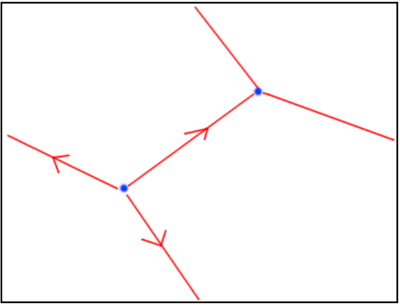
Figure 7. Paths from the boundaries of the curves along the Clifford torus

Remark 4.7.

Let us explain one way to characterize which trivialization fillings are standard. Consider the disks in the symplectization of $(S^{5},\mathbb{T}_{Cl})$ with one positive puncture at the (unique in our presentation) index-1 Reeb chord. Their boundaries trace out paths along ${\mathbb{R}}\times\mathbb{T}_{Cl}$. These were determined (with varying degrees of explicitness) in e.g. [30, 13, 31]; we depict them in Figure 7.

The characteristic topological property of the Harvey-Lawson fillings is that two of the three paths should become isotopic in the filling. This means contracting (in the figure) either the vertical, horizontal, or anti-diagonal circle. One of these is in the same homotopy class as the cusp edge, and the others have intersection numbers $\pm 1$ with it. From Lemma 3.2, we see the latter two give fillings compatible with trivialization. One checks in terms of the rules above that these provide the two different orientations of $\partial D$.

We will give another version of this discussion in terms of a different presentation of the Clifford torus later in Lemma 7.5.

The disk surgery cobordism we created above was trivial outside the surgery region. One might hope that curves which begin and end outside the surgery region behave as if the cobordism was in fact a trivial cobordism. We axiomatize the desired property:

Definition 4.8.

We say that a disk surgery cobordism is weakly perfect if:

1. if there is a nontrivial rigid curve with positive end at Reeb chord $\rho_{+}\in R_{1}(\Lambda_{D})$ and negative end at Reeb chord $\rho_{-}\in R_{1}(\Lambda)$, then $\mathrm{length}(\rho_{+})\geq\mathrm{length}(\rho_{-})$. That is, we ask that these curves respect the action filtration, as they would inside a trivial cobordism. Note we put no condition on curves with negative end at the Clifford torus.

2. There is a unique rigid curve from a each index-1 Reeb chord at the positive end to its counterpart at the negative end, which is a strip whose boundaries become isotopic to vertical lines under the trivialization (8).

By definition, in a weakly perfect disk surgery cobordism for which all chords in $R_{1}(\Lambda)$ and $R_{1}(\Lambda_{D})$ have the same length, the only curves between them which may appear are the trivial strips of (2) above. We axiomatize this:

Definition 4.9.

We say that a disk surgery cobordism is perfect if the only rigid curves between elements of $R_{1}(\Lambda)$ and $R_{1}(\Lambda_{D})$ are one topologically trivial strip between each pair of corresponding chords.

Theorem 4.10.

Suppose that $\Lambda$ and $\Lambda_{D}$ are related by disk surgery, and there exists a perfect disk surgery cobordism $L$ (admitting compatible brane structures), and a standard topological trivialization of $L$. Assume $\partial D$ is not homologically trivial. Fix a completion $\widehat{Sk}(L)$ along a cone containing $\partial D$. Then

$$\mathbf{A}(\Lambda_{D},\rho_{+})\mathbf{E}(\partial D)=\gamma\mathbf{E}(\partial D)\mathbf{A}(\Lambda,\rho_{-})$$

for $\gamma$ some signed monomial in the framing variable.

If we weaken the hypothesis to ‘weakly perfect’, we may still conclude the result for the shortest Reeb chords.

Proof.

Lemma 4.4 plus the perfectness hypothesis gives the following equation:

$$\mathbf{A}(\Lambda_{D},\rho_{+})=\Psi_{Y\times{\mathbb{R}},L}(\rho_{+},\rho_{-})\mathbf{A}(\Lambda,\rho_{-})+\sum_{\nu\in R_{1}(\mathbb{T}_{Cl})}\Psi_{Y\times{\mathbb{R}},L}(\rho_{+},\nu)\mathbf{A}(\mathbb{T}_{D},\nu)$$

where $\rho_{+}$ is a Reeb chord of $\Lambda_{D}$ and $\nu$ runs over the the index $1$ Reeb chords of $\mathbb{T}_{Cl}$. Here, $\Psi_{Y\times{\mathbb{R}},L}(\rho_{+},\rho_{-})$ is the contribution of a trivial strip, hence some signed monomial in ‘$a$’.

We now forget symplectic geometry, and consider the above equation just in the skein of the cobordism. We glue in $\mathbf{T}$ containing $\mathbf{E}$. By the ‘standard’ hypotheses on $\mathbf{T}$, the fact that $\mathbf{E}$ is the skein-valued curve count for a Harvey-Lawson brane [13], and Lemma 4.1, we deduce $\mathbf{A}(\mathbb{T}_{Cl},\nu)\mathbf{E}(\partial D)=0$. We are left with the stated result.

(It may be confusing why the $\mathbf{E}(\partial D)$ appears to the left, rather than right, of $\mathbf{A}(\Lambda,\rho_{-})$, since $\mathbb{T}_{Cl}$ and $\Lambda$ are symplectically both negative ends of the cobordism. The point is that the equation is written in the skein of the ${\mathbb{R}}\times\Lambda$ of Def. 4.5. Here, $\Lambda_{D}$ is at one end, $\Lambda$ at the other, and $\mathbf{T}$ in the middle.) ∎

When we wish to compose cobordisms, we must ensure compatibility of the skein completions. One way to do this is to ask our Legendrians $\Lambda$ to come equipped with an element $\lambda\in H^{1}(\Lambda)$, e.g. given by a 1-form, which match under the topological trivializations of the cobordism, and so that $\lambda(\partial D)>0$ for the various surgeries which appear. We term such cobordisms composable.

Corollary 4.11.

Let $S=(C_{1},C_{2},\ldots,C_{n})$ be a collection of perfect disk surgery cobordisms with standard topological trivializations. Let $C_{i}$ have positive end $\Lambda_{i}$ and negative end $\Lambda_{i-1}$ (union a Clifford torus); assume that the brane structures are also compatible. We write $D_{i}$ and $\partial D_{i}$ for the corresponding surgery disk and its boundary. Suppose given $\lambda_{i}\in H_{1}(\Lambda_{i})$ which agree under the cobordisms and so that $\lambda_{i}(\partial D_{i})>0$.

Then the following expression is well defined

$$\Psi_{S}:=\mathbf{E}(\partial D_{n})\cdots\mathbf{E}(\partial D_{1})\in\widehat{Sk}_{\lambda}({\mathbb{R}}\times\Lambda)$$

Here, $\lambda$ is the common value of the $\lambda_{i}$ and $\Lambda$ the common topological type of the $\Lambda_{i}$.

Moreover,

$$\mathbf{A}(\Lambda_{n})\Psi_{S}=\Psi_{S}\mathbf{A}(\Lambda_{0})$$

In the above situation, we say $\lambda$ controls the composable cobordisms.

Corollary 4.12.

In the situation of Corollary 4.11 suppose the final negative end is $\Lambda_{0}$ has an exact filling $L$. Then the image of $\mathbf{A}(\Lambda)\Psi_{S}$ in $Sk(L)$ is zero.

Proof.

Immediate from Proposition 4.2 and Corollary 4.11. ∎

Remark 4.13.

In practice, often the various $\Lambda_{i}$ will come with their own parameterizations, which match nontrivially (some Dehn twist) under the trivialization of the cobordism. This may lead to the above expression being nontrivial to write in terms of some fixed parameterization of some $\Lambda_{i}$. See e.g. Corollary 9.7 for how this works for cubic planar graph Legendrians.

In the following sections we take on the task of finding conditions which ensure perfectness of disk surgery cobordisms.

Remark 4.14.

Establishing perfectness amounts to excluding certain curves. We will do this by estimating energy. For Lagrangian cobordisms in symplectizations, cylindrical outside some fixed region $M\times[a,b]$, there are (at least) three natural energies to consider, see e.g. [6, 30].

For a curve $u$ with positive Reeb chords $\rho_{1},\dots\rho_{k}$ and negative Reeb chords $\rho^{\prime}_{1},\dots\rho^{\prime}_{l}$, these $3$ energies are:

$$E_{\omega}(u) =e^{b}\sum\ell(\rho_{i})-e^{a}\sum\ell(\rho^{\prime}_{j})$$

$$E_{\lambda}(u) =e^{b}\sum\ell(\rho_{i})$$

$$E(u) =E_{\omega}(u)+E_{\lambda}(u)$$

All of these values are necessarily non-negative. To exclude a holomorphic curve, it therefore suffices to show that one of these would be negative; of course this is in some sense most likely for $E_{\omega}$. However, the most straightforward to estimate is $E$, and it is nontrivial to separate out the $E_{\omega}$ contribution. Compare for instance the two results [30, Lemma 5.1./5.3.] where in one he establishes only an estimate for $E$ and in the other one an estimate for $E_{\omega}$ to rule out some disks. These methods are not sufficient for this text.

However, in the Morse flow tree limit, $E_{\omega}$ has already been separated out. This is why we have been able to prove our results when Morse trees are applicable.

5. Morse flow graphs for cobordisms

Our basic tool for counting curves in the cobordisms will be the adaptations in [8, 7] of the Morse flow tree technology of [5]. We review this below, and then develop some additional results in this context.

5.1. Review of results from [8, 7]

Construction 5.1.

(Morse cobordism, [7, Section 2.3./Remark 3.2.]) Let $\tilde{L}$ be an eventually cylindrical exact Lagrangian cobordism in $(J^{1}(M)\times{\mathbb{R}})$ and denote by $[a,b]$ an interval such that $\tilde{L}\cap(J^{1}(M)\times[a+\epsilon,b-\epsilon])^{c}$ is cylindrical. Then there is an associated Legendrian $L^{Mo}$ in $J^{1}(M\times[e^{a},e^{b}])$ called the Morse cobordism of $\tilde{L}$: Let $\Lambda_{+}=\partial_{\infty}\tilde{L}$ and $\Lambda_{-}=\partial_{-\infty}\tilde{L}$. Furthermore let $h_{+}:[e^{b-\epsilon},e^{b}]\rightarrow{\mathbb{R}}$ be a non-decreasing function fulfilling the following properties:

1. $h_{+}(e^{b})=e^{b}$

2. $h_{+}(e^{b-\epsilon})=e^{b-\epsilon}$

3. $h_{+}$ is given locally around $e^{b}$ by $e^{b}-t^{2}$ and locally around $e^{b-\epsilon}$ by $t+C$ (where $C$ is some positive number).

4. The derivative of $h_{+}$ is $0$ only at $e^{b}$.

We define a similar function $h_{-}:[e^{a},e^{a+\epsilon}]\rightarrow{\mathbb{R}}$. Consider splitting $\Lambda_{+}=(\Pi_{\mathbb{C}}(\Lambda_{+}),z_{+})$ into its Lagrangian projection and Reeb coordinate. Similarly for $\Lambda_{-}$. Then $L^{Mo}$ has the following properties:

1. In a neighborhood of $J^{1}(M\times\{e^{b}\})$ the Morse cobordism is given by:

   $$(h_{+}(t)\Pi_{\mathbb{C}}(\Lambda_{+}),t,h^{\prime}_{+}(t)z_{+},h_{+}(t)z_{+})$$

   where we identify $J^{1}(M\times[e^{a},e^{b}])=T^{*}M\times T^{*}[e^{a},e^{b}]\times{\mathbb{R}}$. A similar statement is true at the negative end.

2. All Reeb chords of $L^{Mo}$ are above $M\times\{e^{a}\}$ or $M\times\{e^{b}\}$. The Reeb chords above the positive end are in $1:1$ correspondence with the Reeb chords of $\Lambda_{+}$ with the index shifted up by $1$. The Reeb chords above the negative end are in $1:1$ correspondence with the Reeb chords of $\Lambda_{-}$ with the same index as in $\Lambda_{-}$.

Proof.

We will need some details of this construction, so we review it here. The main idea is to first identify $J^{1}(M)\times{\mathbb{R}}=T^{*}M\times{\mathbb{R}}\times{\mathbb{R}}$ with $T^{*}(\Lambda)\times T^{*}{\mathbb{R}}_{>0}$ where we choose coordinates $(\lambda,z,t)$ on $J^{1}(M)\times{\mathbb{R}}$ and thus define the following map:

$$\Phi(\lambda,z,t)=(e^{t}\lambda,t,z)$$

One easily verifies that this is a (non-exact) symplectomorphism. We use this symplectomorphism to transport $\tilde{L}$ into $T^{*}M\times T^{*}{\mathbb{R}}_{>0}$. By assumption outside of the interval $[a+\epsilon,b-\epsilon]$ $\tilde{L}$ is cylindrical which means it is given by $\Lambda_{+}\times[b-\epsilon,\infty)$ close to $J^{1}(M)\times\{+\infty\}$. Let $(\Pi_{\mathbb{C}}(\Lambda),z_{+})$ be a parametrisation of $\Lambda_{+}$ then $\Lambda_{+}\times{\mathbb{R}}$ is given by:

$$(\Pi_{C}(\Lambda_{+}),z_{+},t)$$

So the image of $L$ under this symplectomorphism over $T^{*}M\times T^{*}[e^{b-\epsilon},\infty)$ is given by:

$$(t\Pi_{\mathbb{C}}(\Lambda_{+}),t,z_{+})$$

We obtain a similar description over $T^{*}M\times T^{*}(0,e^{a+\epsilon}]$. Now we take the truncation $L^{con}=\Phi(\tilde{L})\cap(T^{*}M\times T^{*}[e^{a},e^{b}])$ and choose a function $h_{+}$ as in the statement of the Construction. One then defines $L^{Mo}$ to coincide with $L^{con}$ except above $M\times[e^{b-\epsilon},e^{b}]$ one deforms $L^{con}$ using $h_{+}$ (and similarly close to the negative end):

$$(h_{+}(t)(\Pi_{\mathbb{C}}(\Lambda_{+}),t,h_{+}^{\prime}(t)z_{+})$$

As $\tilde{L}$ was initially exact, so is $L^{con}$ and one verifies that $h_{+}(t)z$ is an integral of $\alpha_{std}$ of $L^{Mo}$ close to the positive end which can be glued to a lift of $\alpha_{std}$ of $L^{con}$. Thus $L^{Mo}$ lifts to a Legendrian of $J^{1}(M\times[a,b])$ and by abuse of notation we refer to $L^{Mo}$ by this Legendrian.

Reeb chords of $L^{Mo}$ are in bijection with self-intersections of its Lagrangian projection $\Pi_{\mathbb{C}}(L^{Mo})$, and $\tilde{L}$ had no such self-intersections as it was assumed to be an embedded Lagrangian. So away from the neighborhoods where we deformed using $h_{+}$, we have no Reeb chords. In these neighborhoods, we observe that we have Reeb chord above a point $(p,t)$ iff $\Lambda_{+}$ has a Reeb chord above $p$ and $h_{+}^{\prime}(t)(z_{+}(p_{2})-z_{+}(p_{1}))=0$ where $p_{2}$ and $p_{1}$ are the endpoints of the Reeb chord above $p$. For a Reeb chord of $\Lambda_{+}$ we can’t have that $z_{+}(p_{2})=z_{+}(p_{1})$ since this would be an immersed double point. So the above can only be true if $h_{+}^{\prime}(t)=0$ which happens exactly at $e^{b}$ (or $e^{a}$ for $h_{-}$).

The statement about the indices follows directly by observing that the Morse index of a Reeb chord above $\Lambda_{+}$ is increased by $1$: Let $(f_{2}-f_{1})(p^{\prime})=x_{1}^{2}+\dots+x_{k}^{2}-x_{k+1}^{2}\dots-x_{n}^{2}+C$ be a local Morse chart around a Reeb chord of $\Lambda_{+}$. Then in this chart $(f_{2}-f_{1})(x_{1},\dots,x_{n})h(t)=(x_{1}^{2}+\dots x_{k}^{2}-x^{2}_{k+1}-\dots-x_{n}^{2}+C)(e^{b}-t^{2})$ which raises the index by $1$. At the negative end there is a $+t^{2}$ term added so the Morse index remains the same. In addition, if $\gamma$ is a capping path of any such Reeb chord in $\Lambda_{\pm}$ then we can include it into $L^{Mo}$ and obtain a corresponding capping path for the Reeb chord there. So the full index is either shifted up by $1$ or agrees with the initial one. ∎

Our curve counting strategy will be to first count certain curves in $L^{Mo}$ and then use the following result to retranslate it into a statement about curves in the cobordism:

Definition 5.2.

Let $M$ be a any manifold and $g$ a metric on $M\times[e^{a},e^{b}]$ and $L^{Mo}$ be a Morse cobordism in $J^{1}(M\times[e^{a},e^{b}])$ obtained through Construction 5.1. We say that $g$ is pseudo-flat if it fulfills the following properties:

1. Close to $e^{a}$ and $e^{b}$: $g$ decomposes into products $g_{-}+dt^{2}$ and $g_{+}+dt^{2}$.

2. For each Reeb chord $\rho$ of $L^{Mo}$ at the positive end there is a neighborhood $U_{\rho}$ in $M$ such that $g_{+}$ is the Euclidean metric on this neighborhood. Similarly for Reeb chords above the negative end.

3. $g$ has bounded geometry.

Theorem 5.3.

(Disk counting, [7, Lemma 1.4./Theorem 1.5.]) Let $\tilde{L}\subset J^{1}(M)\times{\mathbb{R}}$ be a Lagrangian cobordism cylindrical outside $[a+\epsilon,b-\epsilon]$ and $L^{Mo}$ the associated Morse cobordism from Construction 5.1. For $\gamma\in{\mathbb{R}}$, we write $\gamma L$ for the rescaling of $L\subset J^{1}(M)\times{\mathbb{R}}$ in the fibers of $J^{1}(M)$. Furthermore let $g$ be a pseudo-flat metric. Then there exists:

1. A family $L_{\delta,\sigma}\subset J^{1}(M)\times{\mathbb{R}}$ of eventually cylindrical Lagrangian such that $L_{\delta,\sigma}$ is exact Lagrangian isotopic to $\sigma L$.

2. A family of eventually cylindrical almost complex structures $J_{\delta,\sigma}$.

Then for sufficiently small $\delta,\sigma>0$ there is a $1:1$-correspondence between rigid flow trees with one positive puncture at $L^{Mo}$ defined by $g$ and rigid holomorphic discs with one positive puncture tangent to $L_{\delta,\sigma}$ defined by $J_{\delta,\sigma}$, assuming that the space of rigid flow trees is transversely cut-out.

The restriction that $g$ has to be pseudo-flat is inherited from the study of solutions near Reeb chords of $L_{\delta,\sigma}$ in [7, Section 5]. (In that article, in fact only the case $\dim M=1$ was studied, but as explained to us by Ekholm, the same argument works in general with the pseudo-flat assumption.)

Remark 5.4.

For our applications, we will need to exclude the possibility of higher genus curves. In fact the arguments of [5] already suffice to show that such curves will in this situation limit to flow graphs (see e.g. discussion is [31, Sec. 4]), so showing that there are no flow graphs implies there were no curves. (Note we do not require any transversality or gluing results regarding higher genus flow graphs.)

5.2. Some additional lemmas

In [5] (and so also [8, 7]), it is assumed that all front projections are either two dimensional with generic singularities, or, if higher dimensional, have only cusp-edge singularities. The fronts of (the $L^{Mo}$ of) our cobordisms will be three dimensional, and do not have only cusp edge singularities. So, we cannot directly appeal to [5, Theorem 1.1] to ensure the existence of some deformation of $g$ for which rigid flow trees are transversely cut-out.

Instead, we will have to first directly show that our trees avoid all the singularities other than cusp edges, and are transversely cut out; after this, we can apply the results of [5]. The following lemmas will help us to do this. They hold for Morse flow trees in $L^{Mo}$, without any further assumptions on the geometry of the front projection. (The arguments are essentially trivial, but carried out in sufficient detail as may obscure this fact.)

$L^{Mo}$ close to the boundary decomposes into a product both on the level of the Legendrian and on the level of the metric. This constrains the possibilites for flow graphs considerably. The following Lemma is a sharpening of a statement from [7, Lemma 4.11.]:

Lemma 5.5.

([7, Lemma 4.11.]) Let $L^{Mo}$ be a Morse cobordism and $g$ a metric which decomposes into $g_{\pm}+dt^{2}$ close to the positive/negative end of $L^{Mo}$. Then there are $2$ possible types for connected components of a Morse flow graph:

1. Boundary flow graphs: Flow graphs which are completely contained above $M\times\{e^{b}\}$ or $M\times\{e^{a}\}$. These are in $1:1$ correspondence with the flow graphs of $\Lambda_{+}$ and $\Lambda_{-}$.

2. Interior flow graphs: All edges of the flow graph are above $M\times(e^{a},e^{b})$.

Furthermore, an interior flow graph component has only the following allowed dynamics close to the ends.

1. There are no negative/positive punctures above the positive/negative end.

2. A flow graph close to a puncture $p$ is a multiple cover of the partial flow tree with a single puncture at $p$ and a $1$-valent vertex.

Proof.

Let $\mathcal{G}^{\prime}\subset\mathcal{G}$ be a connected component of a flow graph and let $v$ be a vertex of $\mathcal{G}^{\prime}$ which is above the negative and positive ends and has an adjacent edge which is not contained in that end. Assume that it is above the negative end. Then by Construction 5.1 this cobordism close to the negative end has the form:

$$(h(t)\Pi_{\mathbb{C}}(\Lambda_{-}),t,h^{\prime}(t)z(\Lambda_{-}),h(t)z(\Lambda_{-}))$$

where $\Lambda_{-}$ is an embedding of the negative end into $J^{1}(M)$, $\Pi_{\mathbb{C}}$ is the Lagrangian projection and $z$ is the Reeb chord projection and $h$ is a function which locally looks like $t^{2}$ around $e^{a}$. As the metric decomposes into a product in such a neighborhood the gradient between two sheets looks like:

$$(\gradient(f_{1}-f_{2})(s)h(t),(f_{1}-f_{2})(s)h^{\prime}(t))$$

where $f_{2}$ and $f_{1}$ are locally defined functions (not necessarily on an open subset) around the edge such that $\Lambda$ coincides with the $1$-jet lift of $f_{2}$ and $f_{1}$.

If $t=e^{a}$ then the last coordinate of the differential vanishes; flow lines through any such point are thus contained in the $t=e^{a}$ slice. Consequently, a flow line from the complement of this slice can only limit to the slice if it limits to a critical point. Thus a flow graph vertex on the slice to which a flow line from the slice complement arrives must sit above a Reeb chord, and the flow line from the complement must be carried by the corresponding sheets. Such vertices are always (possibly multiply covered) $1$-valent vertices.

The last statement to show is that there are no negative/positive punctures above the positive/negative end for an interior flow graph component. We will argue that there are no positive punctures above the negative end. The other statement is proven similarly. Consider the local model of a Reeb chord which is given by $(f_{2}-f_{1})(x)h(t)=(x_{1}^{2}+\dots x_{k}^{2}-x_{k+1}^{2}-\dots-x_{n}^{2}+C)(e^{a}+t^{2})$ where $(x_{1},\dots,x_{n})$ are local coordinates on $M$. Then as the metric decomposes into a product, we immediately observe that the unstable manifold of $\gradient(f_{1}-f_{2})h$ is completely contained in the $t=e^{a}$ slice. So any edge limiting away from this puncture will be completely contained in the negative slice. ∎

We now give conditions which ensure that Reeb chords have only trivial flow lines.

Definition 5.6.

Let $\Lambda\subset J^{1}M$ be a Legendrian, and $\rho$ a Reeb chord of $\Lambda$. We say $\Lambda$ is basic around $\rho$ if there is a neighborhood $U\subset M$ beneath $\rho$ such that the following hold over $U$:

1. $\Lambda\to M$ is a covering,

2. The front projection of $\Lambda$ is injective,

3. $\rho$ is the only Reeb chord of $\Lambda$.

Being basic at a Reeb chord is a generic condition on $\Lambda$, which can be expected to fail in codimension one in families.

Definition 5.7.

Let $\tilde{L}$ be an eventually cylindrical Lagrangian cobordism between $\Lambda_{-}$ and $\Lambda_{+}$. Let $\rho$ be a Reeb chord around which $\Lambda_{-}$ is basic for neighborhood $U$. If we have in addition $\tilde{L}\cap(J^{1}(U)\times{\mathbb{R}})=(\Lambda_{-}\cap J^{1}(U))\times{\mathbb{R}}$, then we say that $\tilde{L}$ is basic around $\rho$.

Lemma 5.8.

(Trivial tree) Let $\rho$ be a Reeb chord of $\Lambda_{-}$ and $\tilde{L}$ an eventually cylindrical Lagrangian cobordism which is basic around $\rho$. Furthermore, let $g$ be a metric on $M\times[e^{a},e^{b}]$ such that $g|_{U\times[e^{a},e^{b}]}=g_{-}+dt^{2}$ where $U\times{\mathbb{R}}$ is the cylindrical neighborhood of $\rho$ and $g_{-}$ is a metric on $U$. Then for the associated Morse cobordism $L^{Mo}$ there is a unique flow graph with $1$ positive puncture completely contained in $J^{1}(U\times[e^{a},e^{b}])$ which is a transversally cut-out flow tree and lives in the slice $\rho\times[e^{a},e^{b}]$.

Proof.

Let $\rho$ be a Reeb chord with a neighborhood in $\tilde{L}$ as above. Then there is a neighborhood of $\rho\times[e^{a},e^{b}]$ such that $L^{Mo}$ is the graph of $f_{i}(s)h(t)$ where we chose some local parametrisation of the two sheets of $\Lambda_{-}$ between which the Reeb chord lives. If $f_{2}>f_{1}$ then set $f=f_{2}-f_{1}$. In addition, $h(t)$ is a non-decreasing positive function which locally looks like $t^{2}$ around $e^{a}$ and like $-t^{2}$ around $e^{b}$ whose derivative is $0$ iff $t=e^{a},e^{b}$. As we are using a product metric the gradient of $-f(s)h(t)$ obeys this product structure. As such the gradient in the $M$ direction is dictated by $-h(t)\gradient f(s)$ of $\Lambda_{-}$ and the gradient in the $[e^{a},e^{b}]$-direction is given by $-f(s)h^{\prime}(t)$ which is negative if $t\neq e^{a},e^{b}$ and $0$ if $t=e^{a},e^{b}$. So if $\Lambda_{-}$ has a Reeb chord above the point $s^{\prime}$. Then the gradient given by $(\Lambda_{\Gamma})_{1}-(\Lambda_{\Gamma})_{2}(s^{\prime})$ vanishes. The gradient of $fh$ vanishes on $s\times[e^{a},e^{b}]$ exactly above $s\times\{e^{a}\}$ and $s\times\{e^{b}\}$ and points from the positive to the negative end. Thus, we have a basic Morse flow tree above this line with a positive puncture at $s\times\{e^{b}\}$ and a negative puncture at $s\times\{e^{a}\}$ at the Reeb chords $\rho_{+}$ and $\rho_{-}$ respectively. By the geometric and formal dimension formula from [5, Definition 3.4./3.5.] it follows directly that this flow tree is transversally cut-out.

To finish the proof, we only need to eliminate the possibility that there are any other interior flow graphs. Let $\mathcal{G}$ be any connected flow graph completely contained within this region and $e$ any edge. Then $e$ is oriented in such a way that it points towards the $e^{a}$-slice and no edge of $e$ is ever tangent to a $t$-slice: This can only be possible if $h^{\prime}=0$ or the difference of the functions supporting $e$ vanishes. The first is excluded as we consider an interior flow graph and the other as we consider a neighborhood which has no intersections of function sheets. So the orientation of any edge is always pointing strictly downwards.

Now let $e^{a}=t_{0}<\dots t_{n-1}<t_{n}=e^{b}$ be a decomposition such that all vertices of the flow graph appear on the $t_{i}$-slices. Let $(\tilde{f}_{2}(s)h(t))$ and $(\tilde{f}_{1}(s)h(t))$ be the functions defining those sheets close to an edge living in a slice $U\times[t_{i},t_{i+1}]$. As a shorthand for the function difference we will simply write $e_{H}(s)=(\tilde{f}_{2}(s)-\tilde{f}_{1}(s))$. Now, we define the horizontal energy loss by $H(e)=e_{H}(s_{i+1})-e_{H}(s_{i})$. We immediately, see that the gradient equation of $L^{Mo}$ along each $t$-slice coincides with the respective gradient equation of $\Lambda_{-}$ for these function differences up to multiplication by $h(t)$. So $H(e)$ is a non-negative number as the projection of $e$ is a reparametrisation of the gradient of $e_{H}$ and this number is thus $0$ iff the projection is constant which for a gradient flow is only possible at a Reeb chord. So if $e$ is any edge of the flow graph not projecting to the Reeb chord this will give a positive $H(e)$. Now, if we sum over all $e_{H}$ for any edge which has a contribution above $t_{i+1}$ we obtain:

$$\sum e_{H}(s_{i+1})=\sum e_{H}(s_{i})+\sum H(e)$$

so inductively, we obtain:

$$E(\rho)=KE(\rho)+\sum H(e)$$

which is only possible if $K=1$ and all $H(e)=0$. Meaning that no edge is supported on a sheet different from the ones which support the Reeb chord. Since, we do not consider flow graphs with marked points interior $2$-valent vertices are ruled out and the only possible graph remains the trivial one. ∎

Proposition 5.9.

(Energy bound) Let $L^{Mo}$ be a Morse cobordism above $J^{1}(M\times[e^{a},e^{b}])$ and $B_{\rho}$ be a basic neighborhood of a Reeb chord $\rho$ such that $\hat{L}$ is cylindrical above $B_{\rho}$ and $g+dt^{2}$ a pseudo-flat metric on $M\times[e^{a},e^{b}]$. Then any Morse flow graph G with the condition that (i) $\rho$ is the unique positive puncture and (ii) it leaves $B_{\rho}$ has a minimal energy loss $e^{a}E_{\rho}$.

Proof.

This is almost obvious: Take a slightly smaller neighborhood $B^{\prime}_{\rho}$ and consider a Morse flow graph $G$ as above and restrict it to $(B_{\rho}\setminus B^{\prime}_{\rho})\times[e^{a},e^{b}]$. By $g$-invariance and the cylindrical property. The projection of $G|_{\{B_{\rho}\setminus B^{\prime}_{\rho}\}}$ to $J^{1}(B_{\rho}\setminus B^{\prime}_{\rho})$ consists of a collection of gradient flow lines. As $G$ originally left $B_{\rho}\times[e^{a},e^{b}]$ there must be some sequence of flow lines $(e_{1},\dots e_{n})$ which lift to the upper sheet of the Reeb chord and intersect $\partial B_{\rho}\times[e^{a},e^{b}]$. The length of the sum of the projected flow lines is bounded below by a geodesic and the energy loss is bounded below by the minimum of all gradient differences of all sheets. As we removed a neighborhood of the Reeb chord the norm of the gradient differences is bounded below. Thus, we arrive at an estimate $E$ which is the minimum norm of all gradient differences and the minimal length of a geodesic in the base. To obtain an estimate for the original graph, we must adapt the original gradient equation by multiplying it by $e^{a}$. So $E_{\rho}=\text{min}||\gradient(f_{2}-f_{1})]]d(\partial B_{\rho},\partial B^{\prime}_{\rho})$. ∎

6. Weakly perfect surgery cobordisms for satellites

We will now identify hypotheses which ensure that we can deform $\tilde{L}$ from Construction 3.1 into a Lagrangian cobordism $L$ which is weakly perfect in the sense of Definition 4.8.

To count curves in the cobordism we will use the methods of Theorems 5.3. As a consequence, we are limited to Legendrian cobordisms which are contained in jet bundles, and which moreover have the property that all index 1 Reeb chords of the ends are contained in the jet bundle as well.

Definition 6.1.

Let $\Lambda,\Lambda^{\prime}\subset Y$ be Legendrian surfaces. We say that $\Lambda$ is a satellite of $\Lambda^{\prime}$ if $\Lambda$ is contained in a Darboux neighborhood $U$ of $\Lambda^{\prime}$.

In this case we may consider the fiber rescalings $\Lambda_{\sigma}\subset U$. We say that $\Lambda$ is dominated by $\Lambda^{\prime}$ if $\Lambda^{\prime}$ has no index $1$ Reeb chords and $\Lambda_{\sigma}\subset U$ for all $0<\sigma\leq 1$ has no index $1$ Reeb chords escaping $U$.

Theorem 6.2.

Suppose given some $\Lambda^{\prime}\subset Y$ and some $\Lambda$ dominated by $\Lambda^{\prime}$. Suppose given an admissible surgery disk $D$ for $\Lambda$. Assume in addition:

1. $\Lambda$ is basic (Def. 5.6) around all its index $1$ Reeb chords.

2. The Darboux chart $J^{1}\Lambda^{\prime}$ is compatible with the surgery-defining chart of Figure 3.

3. There are no index-$1$ Reeb chords of $\Lambda$ above the image of $D\subset J^{1}(\Lambda^{\prime})\to\Lambda^{\prime}$.

Then the disk surgery cobordism of 3.1 is isotopic to a weakly perfect disk surgery cobordism.

Proof.

We will count Morse flow trees. Let $\rho_{1},\dots,\rho_{n}$ be an order on the index-$1$ Reeb chords of $\Lambda$ such that the action is non-decreasing. Let $\rho_{i,+}$ denotes the index-$2$ Reeb chord above the positive end and $\rho_{i,-}$ the index-$1$ Reeb chord above the negative end originating from $\rho_{i}$.

Fix a pseudo-flat metric $g+dt^{2}$ on $\Lambda^{\prime}$. Let $E_{1},\dots E_{n}$ be the energy bounds from $g$ as in Proposition 5.9. Let $a<b$ be two real numbers such that $e^{b}\ell(\rho_{j,+})-e^{a}\ell(\rho_{i,-})-e^{a}E_{j}$ is negative if $i\leq j$. This is obviously true if $a=b$ as the order of the Reeb chords was energy non-decreasing. So we can find a pair $(a,b)$ such that this is true for all $i\leq j$.

By Construction 3.1 we find a cobordism of length less than $e^{b-a}$. WLOG the lower end is at $e^{a}=1$. Any Morse flow graph with one positive puncture at $\rho_{j,+}$ and one negative puncture at $\rho_{i,-}$ for $i<j$ must leave a neighborhood of $\rho_{j,+}$ which we used to define the $E_{j}$, and thus have energy more than $E_{j}$. Recall that the energy of a Morse flow graph in such a cobordism is given by $e^{b^{\prime}}\ell(\rho_{j,+})-\ell(\rho_{i,-})$. Since $b^{\prime}\leq b$ this value must also be smaller than $E_{j}$. This is a contradiction, so there could not have been such a curve to begin with. In addition, by Lemma 5.8 there is exactly one flow graph properly contained in such a neighborhood which coincides with the trivial cylinder.

So any other flow graph must leave such a neighborhood, but again the energy constraint of Proposition 5.9 rules out any such graph by a similar argument.

Thus, the flow graph count obeys the following:

1. In the slice $\rho_{i}\times[a,b]$ there is exactly one flow graph with one positive puncture at $\rho_{i,+}$ and one negative puncture at $\rho_{i,-}$. It is homotopic to to a trivial cylinder, and its moduli space is transversely cut out. There are no other Morse flow graphs with these endpoints.

2. If $j<i$ then there are no flow graphs with positive puncture at $\rho_{j,+}$ and negative puncture at $\rho_{i,-}$.

Now Theorem 5.3 asserts the curves for $L_{\sigma,\delta}$ with respect to $J_{\sigma,\delta}$ correspond to the above Morse trees. The above enumerated properties of said trees then translate to the assertion that $L_{\sigma,\delta}$ is weakly perfect. ∎

7. Perfect disk-surgery cobordisms for cubic planar graph Legendrians

We turn to the study of cubic planar graph Legendrians, introduced and studied in [37, 4, 32, 31]. Given an edge $e$ of a graph $\Gamma$, we write $\Gamma_{e}$ for the result of flipping $e$, and also preserve the notation $e$ for the new edge in $\Gamma_{e}$.

Casals and Zaslow have shown that $\Lambda_{\Gamma}$ and $\Lambda_{\Gamma_{e}}$ are related by Legendrian disk surgery [4, Theorem 4.21]. For technical reasons, we cannot directly apply Theorem 6.2 to their construction. Instead, we use other results of the same article [4] to construct a different cobordism, to which we can apply Morse flow technology. Unlike the cobordism of Construction 3.1, this new cobordism will not be arbitrarily short, and we will have to use more of its explicit structure to rule out unwanted Morse flow graphs.

7.1. Cobordism

Construction 7.1.

Consider an unknotted Legendrian sphere $U\subset{\mathbb{R}}^{5}=J^{1}{\mathbb{R}}^{2}$, with the standard flying saucer front in ${\mathbb{R}}^{3}$. We choose it so the base projection to ${\mathbb{R}}^{2}$ has image the unit disk $D_{1}$.

Let $\Gamma$ be a cubic planar graph on $S^{2}$, fix $e$ a distinguished edge of $\Gamma$. Then there is an embedding of $\Lambda_{\Gamma}$ a standard neighborhood of $U\subset{\mathbb{R}}^{5}$ which fulfills the following properties:

1. The base projection of the lift of the graph $\Gamma\subset\Lambda_{\Gamma}$ is contained within $D_{1-\epsilon}$ for the exception of a small neighborhood of the edge $e$ which lies outside of $D_{1-\epsilon}$.

2. The index $2$ Reeb chords are above $D_{\epsilon}$ and the index $1$ Reeb chords are contained above $D_{1-2\epsilon}\setminus D_{\epsilon}$ near the upper hemisphere of $U$.

3. For any pair of sheets with one on the upper and one on the lower hemisphere, all local gradient differences are pointing outward, and are transverse to $D_{\delta}$ for $1-\epsilon>\delta>\epsilon$.

Proof.

The first $2$ conditions can be initially met by observing that the index $1$ Reeb chords are defined by the initial choice of function $f_{\Gamma}$ and then choosing an appropriate identification with the Legendrian unknot $S^{2}\subset{\mathbb{R}}^{5}$.

The second one is easily observed by seeing that if we rescale to some $\sigma\Lambda_{\Gamma}\subset J^{1}(S^{2})$ for small $\sigma>0$, the gradient differences between the upper and lower hemisphere eventually become dominated by the gradients of the upper and lower hemisphere of $S^{2}$ which are non-vanishing for $D_{\delta}$ with $1-\epsilon>\delta>\epsilon$. Thus statement (3) is true and thus for small $\sigma>0$ the statement is also true for $\sigma\Lambda_{\Gamma}$. ∎

We now construct a disk surgery cobordism. Let us first note some differences our previous cobordism in Construction 3.1. Here we use a slightly different presentation of the Clifford torus $\mathbb{T}_{Cl}$, namely as the Legendrian associated to the tetrahedron graph. This allows us to use the Legendrian weave calculus established by Casals-Zaslow [4, Section 4]. Additionally, the non-cylindrical region of the cobordism will not be local to the disk; instead, it sits above the entire front in Figure 8.

Construction 7.2.

Let $\Lambda_{\Gamma}$ be a cubic planar graph Legendrian associated to a graph $\Gamma$ whose front projection satisfies the properties of Construction 7.1. Then for each edge $e$ bounding the large face of $\Lambda_{\Gamma}$ there is an embedding of $\mathbb{T}_{Cl}$ such that there is a cobordism $\tilde{L}$ from $\Lambda_{\Gamma}\sqcup\mathbb{T}_{Cl}$ to $\Lambda_{\Gamma_{e}}$ where $\Gamma_{e}$ is the cubic planar graph obtained from $\Gamma$ by flipping the edge $e$, see Figure 2. In addition, this cobordism is trivial inside $J^{1}(\bar{D}_{1-\epsilon})$ and consists of Legendrian isotopies, an index $1$ and an index $0$-surgery.

Figure 8. The base projection of $\Lambda_{\Gamma}$ containing both the tetrahedron Legendrian (on the right) and a neigborhood of the the edge $e$. Depicted in black are the self-intersections of the front projection coming from $\Gamma\subset S^{2}$ while the grey lines are the self-intersections coming from the inclusion when satelliting $J^{1}(S^{2})\rightarrow S^{5}$. Depicted in red are cusp-edges. The index-$1$ Reeb chords in this area are indicated in green. For a more detailed explanation, see [4].

Figure 9. On the left the resulting Legendrian after the index $0$-surgery which corresponds to a $1$-handle attachment. On the right the resulting simplified Legendrian. This Legendrian is obtained from the original Legendrian by replacing the vertex $v$ with a small triangle.

Proof.

We construct a cobordism as a composition of pieces from [4].

1. Consider a neighborhood $N$ of $e$ as in Figure 8 which also contains the cusp-edges of $\Lambda_{\Gamma}$. Place $\mathbb{T}_{Cl}$ such that the base projection of $\mathbb{T}_{Cl}$ and $\Lambda_{\Gamma}$ are disjoint, see Figure 8. Then we follow the same construction as in [4, Theorem 4.10.4]. Basically this is a Legendrian index $0$ surgery between the outer front cusp-edges, depicted in the Figure on the left of 9. Followed by a Legendrian isotopy resulting in the graphs being “added” along a vertex each where the vertex on $\mathbb{T}_{Cl}$ is chosen arbitrarily and any vertex $v$ adjacent to $e$ will suffice. The two stages after the surgery and after the isotopy are depicted on the right in Figure 9. The resulting Legendrian is associated to the cubic planar graph $\Gamma^{\prime}$ is the same as replacing the chosen vertex $v$ with a triangle where each edge $e_{i}$ formerly attached to $v$ is now attached to a unique vertex of the triangle.

2. The second stage is an index $1$ surgery in the sense of [4, Theorem 4.10.2)]. In our case, we apply it to the edge $e^{\prime}$ connecting the triangle to the former vertex $v^{\prime}$ of $e$ which was not chosen in the previous stage. This move consists of an initial isotopy, an index $1$ surgery and then a final isotopy. We will not in detail describe this isotopy but just remark that it can be made in an arbitrarily small neighborhood of the edge $e^{\prime}$. The resulting Legendrian is depicted on the left of Figure 10.

3. Lastly, the Legendrian right now is not yet a Legendrian associated to a cubic planar graph: In the previous step we introduced an index $0$ Reeb chord on the face obtained from the triangular face and the ”opposite” face before. However, as can be seen in Figure 10. There is an additional index $1$ Reeb chord inherited from the triangular face. So a final isotopy is designed to merge this index $0$ and index $1$ Reeb chord. Again, this can be done outside $\bar{D}_{1-\epsilon}$. After this final isotopy, we have obtained a Legendrian which is associated to a cubic planar graph $\Gamma_{e}$ obtained from $\Gamma$ by flipping the edge $e$. This Legendrian is depicted on the right of Figure 10.

∎

Figure 10. On the left the Legendrian obtained from index $1$ surgery. The additional index $0$ Reeb chord is depicted in light green. On the right is the Legendrian after a small isotopy cancelling the Reeb chords and normalising the picture. This Legendrian has all the original Reeb chords.

The first stage of the above cobordism will be called the “Clifford sum” cobordism (following [4, Theorem 4.10]) at the vertex $v$ which was chosen.

Figure 11. Proof of Lemma 7.3. Left: the negative end of the cobordism. Middle: after index zero surgery. Right: after index one surgery. Note that the two positively oriented lifts of the edges at the negative end of the edges have opposite orientation when oriented to the positive end.

Lemma 7.3.

If we depict the cobordism as a movie of base projections, we see one of the edges $e_{T}$ of the tetrahedron graph get connect summed with the edge $e$ of $\Gamma$.

Then the associated cycles $[-e_{T}]\in H_{1}(\mathbb{T}_{Cl})$ and $[e]\in H_{1}(\Lambda)$ have the same image in

$$H_{1}(\mathbb{T}_{Cl})\to H_{1}(\widetilde{L})\leftarrow H_{1}(\Lambda)$$

Proof.

Note the cycles associated to opposite edges of the tetrahedron graph agree up to a shift in orientation. Now the proof is given in Figure 11. ∎

7.2. Perfectness

We now show the curve count in the Morse cobordism $L^{Mo}$ associated to $\tilde{L}$ is perfect.

We fix notation. The positive end of $L^{Mo}$ coincides with $\Lambda_{\Gamma_{e}}$ and the negative end with $\Lambda_{\Gamma}\sqcup\mathbb{T}_{Cl}$. By construction the set $J^{1}(D_{1-\epsilon})$ contains all Reeb chords of $\Lambda_{\Gamma}$ and of $\Lambda_{\Gamma_{e}}$ (contained within the initially chosen Darboux chart ${\mathbb{R}}^{5}\subset S^{5}$) and the cobordism is cylindrical above this set. Thus the set of Reeb chords are in $1:1$ correspondence. Each of which gives rise to two Reeb chords in $L^{Mo}$ one above the positive end and one above the negative end. For the Reeb chord above the negative end the index coincides with the index as in $\Lambda_{\Gamma}$ while the index for the positive end is raised by $1$. These will be denoted by $\rho_{+}$ and $\rho_{-}$, respectively.

Theorem 7.4.

The disk surgery cobordism of Construction 7.2 is isotopic to a perfect disk surgery cobordism.

Proof.

Let $L^{Mo}$ be the Morse cobordism obtained from the eventually cylindrical cobordism $\tilde{L}$ from the construction. Let $\rho_{i}$ ($i=1,2$) be two index $1$ Reeb chords of $\Lambda_{\Gamma}$. Endow $T^{*}({\mathbb{R}}\times[a,b])$ with the Euclidean metric.

We will show that the space of Morse flow graphs with one positive puncture at $\rho_{1,+}$ and a negative puncture at $\rho_{2,-}$ is empty if $\rho_{1}\neq\rho_{2}$. If $\rho_{1}=\rho_{2}$ then it contains the trivial Morse flow tree and no other Morse flow graphs. In particular, these spaces of Morse flow graphs are transversally cut-out. Thus, we obtain a perfect disk surgery cobordism via Theorem 5.3.

By Construction 7.1 $\Lambda_{\Gamma}$ is basic around all its Reeb chords and by Construction 7.2 the cobordism $\tilde{L}$ is cylindrical above $\bar{D}_{1-\epsilon}\times{\mathbb{R}}$. So in particular $\tilde{L}$ is basic around all Reeb chords of $\Lambda_{\Gamma}$. So, we may use Lemma 5.8 with respect to the euclidean metric on $M\times[e^{a},e^{b}]$ and obtain that the space of Morse flow graphs with unique positive puncture at $\rho_{+}$ and unique negative puncture at $\rho_{-}$ contains the trivial Morse flow tree for any Reeb chord $\rho$ of $\Lambda_{\Gamma}$ and they are transversely cut-out. To obtain the theorem, we only have to rule out rigid Morse flow graphs which have a unique positive puncture at a Reeb chord $\rho_{i,+}$ and a negative puncture at a negative Reeb chord $\rho_{j,-}$ which is not the same as the trivial tree. We will show this by proving that a Morse flow graph having a negative puncture at $\rho_{j,-}$ must have a positive puncture at $\rho^{\prime}_{+}$ coming from an index $2$ Reeb chord of $\Lambda_{\Gamma}$.

Let $G$ be an interior Morse flow graph with a negative puncture at $\rho_{j,-}$. From Lemma 5.5 we obtain that the flow graph close to a puncture above $\rho_{j,-}$ must look like a multiple cover of a leaf which is oriented towards the puncture. Either all covers of that edge continue up the trivial flow line ($\subset\rho\times[e^{a},e^{b}]$) to $\rho_{j,+}$ and take it as a positive puncture multiple times or there is an internal vertex $v$ which has an adjacent edge whose $1$-jet lift includes one of the sheets of the lower hemisphere. Recall that by the definition of a Morse flow graph there must be a cyclic order on the edges adjacent to a (non-puncture) vertex $v$. This obeys the rule that an inward pointing edge must be followed (or preceded) by an edge which lifts to the same sheet but is outward pointing. Thus we claim that there must be some edge $e$ pointing to $v$ which has one $1$-jet lift on the upper hemisphere and one lift on the lower hemisphere (See the next paragraph). By Construction 7.1 these gradients are all transverse to $\partial D_{\delta}$ for some $\delta>\epsilon$. Thus as we follow $e$ up its radius will shrink. Each time we meet a vertex of $G$ we find another edge $e^{\prime}$ which fulfills the same condition. Until we are inside $D_{\epsilon}$ which by assumption a mixed gradient flow line cannot enter. Now denote by $T$ the maximum value of the projection to $[e^{a},e^{b}]$ any gradient flow line of $\mathcal{G}^{\prime}$ achieves inside $D_{\delta}$. This cannot be achieved on the interior of an edge and if it were to be on a non-puncture vertex then we could find another flow line which we can follow upwards and achieve a value $T^{\prime}>T$ in its interior. This is only possible if $T=e^{b}$, but by the argument in the proof of Lemma 5.5, this cannot happen for a non-puncture vertex. Thus we have successfully ruled out Morse flow graphs which are not of the desired type.

It remains to prove the claim that if we have a non-puncture vertex $v$ with an outgoing edge $e$ which is supported by one sheet of the upper hemisphere and one of the lower hemisphere then there must be an ingoing edge $e^{\prime}$ fulfilling the same restriction (with possibly different upper or lower sheets). Above any point $p$ in $D_{\delta}$ $0<\delta<1-\epsilon$ we have $4$ sheets which we will denote by $U^{1},U^{2},L^{1},L^{2}$ where $U^{i}$ are the two sheets of the upper hemisphere and $L^{i}$ are the two sheets of the lower hemisphere. Furthermore denote by $U^{i}_{\pm}$ and $S^{i}_{\pm}$ the number of incoming directions ($U^{i}_{+}/S^{i}_{+}$) and the number of outgoing directions ($U^{i}_{-}/S^{i}_{-}$) at $v$. The restriction that there is a cyclical order on the edges adjacent to any vertex implies that an incoming lift of an edge $e_{i}$ on some sheet must be followed (or preceded) by an outgoing lift on the same sheet, implies $U^{i}_{+}=U^{i}_{-}$ and $S^{i}_{+}=S^{i}_{-}$ for $i=1,2$. Now consider the weighted sum $U_{w}=U^{1}_{+}+U^{2}_{+}-U^{1}_{-}-U^{2}_{-}$ and similarly $S_{w}=S^{1}_{+}+S^{2}_{+}-S^{1}_{-}-S^{2}_{-}$ both of these numbers must be $0$. Note however, that edges supported either by both upper or lower sheets doesn’t change the sums. However, if we have a mixed outgoing edge this contributes $-1$ to $S_{w}$ and $1$ to $U_{w}$. So a mixed incoming edge is necessary. ∎

7.3. Filling the Clifford torus

Consider the Legendrian $\mathbb{T}_{Cl}\subset S^{5}$ associated to the tetrahedron graph. Each edge of the graph determines a cycle on $\mathbb{T}_{Cl}$; in fact opposite edges give the same cycle. Let us denote the resulting cycles $\ell,m,n$; one has $\ell+m+n=0$, and any two give a basis of $H_{1}(\mathbb{T}_{Cl})$.

There are three topologically distinct families of Lagrangian fillings of $\mathbb{T}_{Cl}$, coming from different smoothings of the Harvey-Lawson cone. Each of the three fillings contracts exactly one of these cycles. If a given filling contracts $\ell$, then in that filling $m=-n$, and one of these is positive with respect to the primitive of the symplectic form. Moreover, the other two fillings render $\ell$ respectively positive or negative with respect to the primitive of the symplectic form on ${\mathbb{C}}^{3}$.

These fillings may be glued topologically to the Clifford torus end of a cobordism coming from Construction 7.2. We refer to this construction as a topological Harvey-Lawson filling.

Lemma 7.5.

Consider the three possible topological Harvey-Lawson fillings of the Clifford torus. These each contract a different one of the three cycles $\{\ell,m,n\}\in H_{1}(\mathbb{T}_{Cl})$; denote the contracted cycle $\gamma$.

Let $e_{T}$ be the edge from Lemma 7.3. Then the intersection pairing $(\gamma,e_{T})$ takes the three values $+1,0,-1$, one on each filling. We refer to the corresponding fillings as positive, forbidden, and negative, respectively.

Moreover, on the positive and negative fillings, the topological result of gluing in the Harvey-Lawson filling is a trivial cylinder; this being false for the forbidden filling.

Proof.

Proven similarly to Lemma 3.2. Note that in that proof we require that the index $2$ Morse singularity of the cobordism $L_{e}$ and the index $1$ Morse singularity in $\mathbf{T}_{Cl}$ are cancellable. This is only possible if (after some choice of metric) their stable and unstable manifolds have one algebraic intersection. As the unstable manifold of the index $2$ manifold is homotopic to the $e+e_{T}$ cycle and the stable manifold is homotopic to the contractible cycle. This is impossible if $e_{T}$ is the contractible cycle. If $e_{T}$ is not the contractible cycle it is some generator of homology and thus has one algebraic intersection with the contractible cycle. ∎

7.4. Proof of Theorem 1.3

We now establish the result:

Theorem 7.6.

Let $\Gamma$ be a cubic planar graph, and $e$ a non-loop edge of $\Gamma$. We write $e^{+}$ for the corresponding oriented simple closed curve, and $e^{-}$ for the curve with opposite orientation. Then we have the following equations, holding, respectively, in completions of the skein in the directions of $e_{+}$ and $e_{-}$:

$$\mathbf{A}(\Lambda_{\Gamma_{e}})\mathbf{E}(e_{+})=\mathbf{E}(e_{+})\mathbf{A}(\Lambda_{\Gamma})$$

$$\mathbf{A}(\Lambda_{\Gamma_{e}})\mathbf{E}(e_{-})=\mathbf{E}(e_{-})\mathbf{A}(\Lambda_{\Gamma})$$

Proof.

In Theorem 7.4, we have constructed perfect cobordisms for the Legendrian disk surgeries associated to mutations of cubic planar graphs. Lemma 7.7 provides each with two standard trivializations, one inducing each orientation of the loop corresponding to $e$. Now the result follows from Theorem 4.10. ∎

8. The necklace graph

The “necklace graph” $\Lambda_{Neck,g}$ (see Fig. 12) has the virtue that its associated Legendrian has an exact filling which is topologically the genus $g$ handlebody [4, Theorem 4.10.1, Theorem 4.17].

Several of the main results of [32] concern properties of sequences of q-cluster transformations associated to sequences of graph mutations beginning with the necklace graph, and having a certain positivity property. We will give geometric counterparts of said results here, and correspondingly prove that certain explicit skein-valued lifts of the formulas written in [32] are in fact skein-valued curve counts.

Figure 12. The necklace graph of genus $g$.

8.1. Lemma on skeins of handlebodies

Let $L_{g}$ be a handlebody of genus $g$, with boundary $\Sigma_{g}$. The following result is presumably well known, although we did not find a reference:

Lemma 8.1.

Fix a disk $D\subset L_{g}$. If $\Psi\in Sk(L_{g})$ satisfies $(1-\partial D)\Psi=0$, then $\Psi$ is the image of an element of $Sk(L_{g}\setminus D)$.

Proof.

The connect sum theorem of [23] asserts that $Sk(A\#B)=Sk(A)\otimes Sk(B)$ (after inverting the q-numbers $[n]_{q}=1-q^{n}$, which we have done from the outset).

We view the handlebody as the connect sum of a handlebody of genus one less and a solid torus containing $D$. The connect sum theorem then reduces the lemma to the case of the solid torus. Now the result follows from the fact that the skein of the solid torus admits a basis in the meridian acts diagonally, and the $1$-eigenspace consists of only the constants; see e.g. [26]. ∎

Remark 8.2.

The proof of the connect sum theorem [23] uses the full strength of many results in skein theory, such as [2, 29]. We expect the lemma has a more elementary proof.

Fix $\lambda\in H^{1}(L_{g})$. We write $Sk^{\geq 0}(L_{g})$ for the elements on which $\lambda\geq 0$, and $Sk^{>0}(L_{g})$ for the strictly positive elements.

Lemma 8.3.

Let $c$ be a simple closed curve on $\Sigma_{g}$. Let $\Psi\in 1+\widehat{Sk}_{\lambda}^{>0}(L_{g})$. If $(\bigcirc-c)\Psi=0$, then $c$ must bound in $L_{g}$.

Proof.

If $\lambda(c)<0$, then the leading term of $(\bigcirc-c)\Psi$ is $c\neq 0$. If $\lambda(c)>0$ then the leading term is $\bigcirc\neq 0$. Thus $\lambda(c)=0$, and the leading term is $\bigcirc-c$. As this must vanish in $Sk(L_{g})$, we conclude $c$ bounds. ∎

8.2. Curve counts and the necklace graph Legendrian

Figure 13. We describe the element $\mathbf{A}(f)$, when $f$ is a bigon face of a graph $\Gamma$, by specializing [31, Figure 7]. What is drawn is the region of $\Lambda_{\Gamma}$ above a neighborhood of $f$; the outer two $6$-valent vertices are identified with one another. In black are the lifts of the edges of the graph $\Gamma$, in blue the tangles of $\mathbf{A}(f)$, in red a choice of capping path we used in [31, Figure 7].

We recall a very special case of the main theorem of our previous article [31]. For the Reeb chord $\rho$ associated to a bigon of $\Lambda_{Neck,g}$, and $E_{i}$ either edge of the face, one has

(9) $$\mathbf{A}(\rho)=a^{-1}\bigcirc+[E_{i}].$$

See Figure 13.

Remark 8.4.

The explicit formula for $\mathbf{A}(\rho)$ may be confusing: on the one hand, the unknot and $[E_{i}]$ become isotopic in the filling, and on the other, we have claimed the image of $\mathbf{A}(\rho)$ is zero. The point is that we are working in a skein with sign/linking lines. What necessarily happens in the filling is that $[E_{i}]$ must cross some such lines as it is contracted, introducing an appropriate power of $-a$, in this case $-a^{-1}$.

Figure 14. The necklace graph $\Lambda_{Neck,2}$, and a collection of disks whose lifts to $\Lambda_{\Gamma_{Neck,2}}$ give disconnecting cylinders.

Lemma 8.5.

Choose one edge of the bigons of the necklace graph. The corresponding cycles separate $\Lambda_{\Gamma_{Neck,g}}$ into two punctured disks.

Proof.

A small thickening of these cycles branch-cover a small neighborhood of the corresponding edges. In the complement of these neighborhoods, the map $\Lambda_{\Gamma_{Neck,g}}\to S^{2}$ is an unbranched cover, which one sees by inspection is disconnected. See Figure 14. ∎

Corollary 8.6.

Let $L$ be any genus $g$ handlebody filling $\Lambda_{Neck,g}$. Fix any $\lambda\in H_{1}(L)$. If $\Psi\in 1+\widehat{Sk}_{\lambda}^{>0}(L)$ and $\mathbf{A}(\Lambda_{Neck,g})\Psi=0$, then $\Psi=1$.

Proof.

We pull the sign/linking lines past the $\mathbf{A}(\Lambda_{Neck,g})$ so that the expression (9) for the generating elements becomes the more familiar $\bigcirc-[E_{i}]$. By Lemma 8.3, the $E_{i}$ appearing in the formula (9) bound disks in the filling. Since, per Lemma 8.5, these cycles separate $\Lambda_{Neck,g}$ into two punctured disks, we may ensure the disks in the filling correspondingly separate the filling into two balls.

Iteratively applying Lemma 8.1 implies that image of $\Psi$ in $L_{g}$ is in the skein of a ball, hence is a scalar. Finally, the leading term of $\Psi$ is the scalar $1$, so we are done. ∎

Theorem 8.7.

Let $S=(C_{1},\ldots,C_{n})$ be a composable sequence of cobordisms, with positive end $\Lambda$ and negative end $\Lambda_{Neck,g}$. Let $L$ be the topological filling of $\Lambda$ obtained from the standard filling $L_{g}$ of $\Lambda_{Neck,g}$ by the smooth identification $\Lambda\cong\Lambda_{Neck,g}$ using the trivialization of $S$.

Assume the controlling $\lambda\in H_{1}(\Lambda)$ vanishes on meridians of $\Lambda_{Neck,g}$ hence extends to $L$.

Then $\mathcal{A}(\Lambda)\Psi=0\in\widehat{Sk}_{\lambda}(L)$ has a unique solution with $\Psi\in 1+\widehat{Sk}_{\lambda}^{>0}(L)$, namely the image of $\Psi_{S}$ in $\widehat{Sk}_{\lambda}(L)$.

In particular, in case $(L,\lambda)$ is diffeo rel boundary to some geometric filling $L_{geom}\subset{\mathbb{R}}^{6}$, and $\lambda$ is the restriction of the symplectic primitive, then $\Psi_{S}$ is the skein-valued curve count of curves ending on $L_{geom}$.

Proof.

By Corollary 4.2, $\Psi_{S}$ is indeed a solution. Suppose given some other solution, $\Psi$. We multiply $\mathbf{A}(\Lambda)\Psi=0$ by $\Psi_{S}^{-1}$ (note the inverse exists as usual for something in a completion with invertible leading term). Then we have

$$0=\Psi_{S}^{-1}\mathbf{A}(\Lambda)\Psi=\mathbf{A}(\Lambda_{Neck,g})\Psi_{S}^{-1}\Psi$$

Now $\Psi$ has leading term $1$ by hypothesis, and $\Psi_{S}$ is the product of elements with leading term $1$, so also $\Psi_{S}^{-1}\Psi$ has leading term $1$. By Lemma 8.6, $\Psi_{S}^{-1}\Psi=1$. Applying $\Psi_{S}$ on both sides, we have $\Psi_{S}=\Psi$. ∎

9. Composable cobordisms from admissible mutations

In order to apply our results on composable cobordisms (Corollary 4.11, Theorem 8.7), we need to check when sequences of cobordisms are composable.

In particular, suppose given some cubic planar graph $\Gamma=\Gamma_{0}$, putative controlling element $\lambda\in H_{1}(\Lambda_{\Gamma})$, sequence of edges $e_{1},e_{2},\ldots,e_{n}$ and sequence of signs $\epsilon_{1},\epsilon_{2},\ldots,\epsilon_{n}\in\{\pm\}$. We write $\Gamma_{i}$ for the graph obtained by mutating $\Gamma_{i-1}$ at $e_{i}$. We write $C_{i}$ for the corresponding disk surgery cobordism of sign $\epsilon_{i}$ (recall the sign prescription in Lemma 7.5).

We would like an algorithmic way of deciding when the sequence $(C_{1},C_{2},\ldots,C_{n})$ is a composable sequence controlled by $\lambda$. In other words, we should check when the class of the circle $[e_{i-1}]\in H_{1}(\Gamma_{i})$ are all positive for $\lambda$ under the identifications $H_{1}(\Gamma)=H_{1}(\Gamma_{i})$ induced by the cobordism trivializations.

The main difficulty in doing so is to give an expression for how the homology transforms under the cobordism trivializations. Fortunately, this was already done in [32]. We recall their result (which however was proven for a somewhat different presentation of the cobordisms, so we provide a proof in our context).

Lemma 9.1.

[32] Let $\Lambda_{\Gamma}$ be a CPG Legendrian and $e\in\Gamma$ an edge. Fix a positive topological Harvey-Lawson filling of the cobordism $L$ associated to the edge $e$. Then the isomorphism $H_{1}(\Lambda_{\Gamma_{e}})\xrightarrow{\sim}H_{1}(\Lambda_{\Gamma})$ is given by the following formulas for homology classes of loops associated to edges of the respective graphs where $\tilde{e}^{\prime}$ denotes the edge corresponding to $e^{\prime}$ after the edge flip at $e$:

$$\tilde{e}^{\prime}\mapsto e^{\prime} e^{\prime} e$$ not adjacent to

$$\tilde{e}\mapsto -e$$

Let $e_{1},\dots e_{4}$ be the edges adjacent to $e$ such that, in the counterclockwise cyclic order at vertices, $e_{2}$ and $e_{4}$ precede $e$ and $e_{1},e_{3}$ come after $e$, see Figure 15. Then the induced map satisfies also:

$$\tilde{e}_{i}\mapsto e_{i} i=1,3$$

$$\tilde{e}_{i}\mapsto e_{i}+e i=2,4$$

We obtain a similar map for negative mutation just that the last set of equation is changed to:

$$\tilde{e}_{i}\mapsto e_{i}+e i=1,3$$

$$\tilde{e}_{i}\mapsto e_{i} i=2,4$$

Figure 15 also depicts this map for the edges around $e$.

Figure 15. Positive and negative mutation of edge labels, per [32].

Figure 16. On the left a neighborhood of the edge $e$ and a tetrahedron graph with a choice of basis coming from the chosen smoothing such that $V=0$. In the middle after identifying the lower edge of $\Gamma$ and the lower left edge of the tetrahedron graph. On the right the result after gluing in the disk which sets $e-U=0$.

Proof.

We will do the calculation in the case of positive mutation. The case of negative mutation is proven similarly.

First, let us consider what happens in the first stage of the Cobordism from Construction 7.2. This corresponds to the “Clifford sum” cobordism. In particular, the cobordism is a cylinder in a neighborhood of all edges not adjacent to the two vertices which merge. As we chose positive mutation the gluing can be done as indicated in the middle of Figure 16. The other cases of positive mutation are proven similarly. As this part of the cobordism only concerns a neighborhood of the two merging vertices, we record that this cobordism maps all other edges by the identity. The same is true for the remaining edges of the tetrahedron graph Legendrian. Now, recall that each face must fulfill the condition that the product over all edges adjacent to a face must vanish. So we obtain the equation for the remaining $3$ edges:

$$(\Sigma_{e^{\prime}\in F,e^{\prime}\neq e_{i},e_{j}}e^{\prime})+e_{i}+e_{j} =0 i,j\in\{0,3,4\} ,i\neq j$$

$$(\Sigma_{e^{\prime}\in F,e^{\prime}\neq e_{i},e_{j}}e^{\prime})+\phi(e_{i})+\phi(e_{j})+e_{i,j} =0 i,j\in\{0,3,4\} ,i\neq j$$

where $e=:e_{0}$, $e_{3,4}=-U$, $e_{0,3}=U$ and $e_{0,4}=0$. $i,j$ are considered to be unordered. Setting the corresponding pairs equal, we obtain the following equation:

$$\phi(e_{0})+\phi(e_{3})+U =e_{0}+e_{3}$$

$$\phi(e_{3})+\phi(e_{4})-U =e_{3}+e_{4}$$

$$\phi(e_{4})+\phi(e_{0}) =e_{4}+e_{0}$$

A straightforward verification shows:

$$\phi(e_{0}) =e_{0}-U$$

$$\phi(e_{3}) =e_{3}$$

$$\phi(e_{4}) =e_{4}+U$$

Next, we consider the result of the $1$-surgery which corresponds to gluing in a $2$-disk. Again all edges not adjacent to it just propagate upwards, so the homology map maps them by the identity. Furthermore, it kills the $\phi(e)$ edge which enforces on the homology level the equation $e_{0}-U=0$. So the edge labeled $-U$ from $\Lambda_{\Gamma_{v}}$ can now be labeled $-e$. Finally, we are left with labeling the two remaining edges: To do so, we consider $e_{1}+\phi(e_{0})+U$ and $e_{2}+\phi(e_{0})+U$ which is represented by a loop which goes from one end of the triangle around $\phi(e_{0})$ to the end of either $e_{1}$ or $e_{2}$. As can be seen in Figure 16. These avoid the edge which vanishes by the surgery. So finally $\phi$ can be modified by: $\phi(e_{1})=e_{1}$, $\phi(e_{2})=e_{2}+e$ and $\phi(e_{0})=-e_{0}$. ∎

For comparison with [32], let us recall their definition of ‘admissible sequence of mutations’.

Definition 9.2.

([32]) Let $(U_{j},V_{j})$ be the basis for $H_{1}(\Gamma_{Neck})$ in which the classes of the cycles associated to the edges are as depicted in Figure 17. We will call this the standard basis for the necklace graph Legendrian.

Let $(e_{1},\dots e_{n})$ be a sequence of edges and $(\epsilon_{1},\dots,\epsilon_{n})$ a sequence in $\{1,-1\}$. Consider the sequence $\Gamma_{0}=\Gamma_{Neck,g}$, $\Gamma_{i}=(\Gamma_{i-1})_{e_{i}}$. This is said to be admissible if the homology class of $\epsilon_{i}e_{i}$ written in the basis $(U_{j},V_{j})$ has no negative coefficients in the $U_{j}$, and at least one of said coefficients is positive.

Remark 9.3.

The ‘seeds’ of [32] are q-lifts of the choice of homology basis, and their transformation relation [32, Figure 4.2.2., page 20/21] is compatible with Lemma 9.1.

We translate this as follows:

Lemma 9.4.

Let $\lambda\in H^{1}(\Lambda_{\Gamma_{Neck}})$ vanish on the $V_{j}$ and be positive on the $U_{i}$. If a sequence $(e_{1},\dots,e_{n})$ and $(\epsilon_{1},\dots,\epsilon_{n})$ defines an admissible sequence of mutations then the corresponding sequence of disk surgery cobordisms is composable and controlled by $\lambda$. Conversely, if the sequence is composable for all such $\lambda$, then it is admissible.

Proof.

Consider the induced $1$-form $\lambda^{\prime}$ on $\mathbf{T}$ which is given by $\lambda(e_{i}+e_{T})=0$ and thus $\lambda^{\prime}(e_{T})=-\lambda(e_{i})$ where $e_{T}$ is the edge from Lemma 7.3. Note that in the case of positive mutation, see Figure 16, the edge $e_{T}$ succeeds (in the anticlockwise cyclical order) the contractible edge $\gamma$. Thus by the intersection pairing for their lifts $(\gamma,e_{T})=-1$ and thus $(\gamma,\cdot)=-\lambda^{\prime}$ which by Lemma 7.5 implies that we can positively fill the associated cobordism. So if $\lambda$ evaluates positively on $e_{i}$ we can compose the positive mutation cobordism. One proves the case for negative mutation similarly. ∎

Remark 9.5.

We see from Lemma 9.4 that the notion of composable cobordism is much more general than that of admissible mutation, even in the context of cubic planar graphs.

The following is useful in calculations:

Lemma 9.6.

Let $(e_{1},\ldots,e_{n})$ and $(\epsilon_{1},\ldots,\epsilon_{n})$ be the edges and signs defining a composable sequence $S$ of mutations beginning at the necklace graph, and let $(e^{\prime}_{1},\ldots,e^{\prime}_{m})$ and $(\epsilon^{\prime}_{1},\ldots,\epsilon^{\prime}_{m})$ be another, call it $S^{\prime}$.

Assume that the two mutation sequences induce the same map in homology. Then $\Psi_{S}=\Psi_{S^{\prime}}\in\widehat{Sk}(L)$, where $L$ is the standard filling of the necklace graph Legendrian.

Proof.

The force of the lemma is that we do not assume that the trivializations induce the same map on simple closed curve classes, so we can’t simply invoke the uniqueness result of Theorem 8.7 directly.

Instead, we reason as follows. Since the maps are the same in homology, it follows that in fact $(e_{1},\ldots,e_{n},\tilde{e}_{m},\ldots,\tilde{e}_{1})$ and $(\epsilon_{1},\ldots,\epsilon_{n},-\epsilon^{\prime}_{m},\ldots,-\epsilon^{\prime}_{1})$ define a composable sequence, now from the necklace graph to itself. We write $\overline{S}^{\prime}$ for the second half of this sequence.

By Corollary 4.12, we find that the image of $\Psi_{\overline{S}^{\prime}}\Psi_{S}$ in $\widehat{Sk}(L)$ is annihilated by $\mathbf{A}(\Lambda_{Neck})$. Now by Theorem 8.7, we may conclude $\Psi_{\overline{S}^{\prime}}\Psi_{S}=1\in\widehat{Sk}(L)$. On the other hand, we may apply exactly the same reasoning to conclude $\Psi_{\overline{S}^{\prime}}\Psi_{S^{\prime}}=1\in\widehat{Sk}(L)$. Cancelling on the left gives the desired result. ∎

Figure 17. The necklace graph of genus $g$ with a special choice of basis. (The quantum torus version of this basis appears in [32, page 54].)

We will now study how the diffeomorphism $\Lambda_{\Gamma}\cong\Lambda_{\Gamma_{e}}$ act on isotopy classes of simple closed curves, rather than just on homology.

Lemma 9.7.

Fix an edge $e$ of a CPG $\Gamma$. We consider the mutation at $e$. As always, denote by $[\mathrm{edge}]$ the oriented closed curve associated to the edge. We preserve the notations $\tilde{e}$, $e_{i}$, $\tilde{e}_{i}$ from Lemma 9.1.

Under the diffeomorphism $\Lambda_{\Gamma}\cong\Lambda_{\Gamma_{e}}$, we find that $[\tilde{e}]$ is the same curve as $[e]$ but with reversed orientation.

If the mutation was positive then for $i=1,3$ the closed curves $[\tilde{e}_{i}]$ and $[e_{i}]$ are homotopic while if $i=2,4$ $[\tilde{e}_{i}]$ is the Dehn twist of $[e_{i}]$ around $[e]$. If the mutation is negative then the two cases are reversed.

Figure 18. Neighborhoods of the edges $e$ and $\tilde{e}$. Indicated in red is the curve which has two lifts both of which lift to a neighborhood of the boundary. Note that the curve on the left is the positively oriented lift of $e$ while the curve on the right is the negatively oriented lift of $\tilde{e}=-e$.

Figure 19. On the left the annulus $A$ from Figure 18 when viewed on the surface underlying $\Lambda_{\Gamma}$ and $\Lambda_{\Gamma_{e}}$. Indicated in black and red are the double lifts of the edges within this neighborhood. On the left pre-surgery and on the right after positive (above), resp. negative (below) mutation. In red are the curves which transform by Dehn twist while in black are the ones which do not.

Proof.

Basically the point is that the transformation is confined to an annulus, and in an annulus the action on relative homology determines the action on the space of simple paths.

In more detail, the statement about $[e]$ and $[\tilde{e}]$ is proven in Figure 11. To observe the other case, let us fix positive mutation and a topological trivialisation of $L_{e}\#\mathbf{T}\cong\Lambda_{\Gamma}\times{\mathbb{R}}$ as in Lemma 7.5. Outside the annulus $A$ indicated in Figure 18 this trivialisation coincides with the cylindrical structure of $(\Lambda_{\Gamma}\setminus A)\times{\mathbb{R}}$ and with $\Lambda_{\Gamma}\times(-\infty,-R]$ and $\Lambda_{\Gamma_{e}}\times[R,\infty)$ for $R$ large enough. Outside of the cylinder $A\times{\mathbb{R}}$ the double lifts of $e_{1},\dots,e_{4}$ and $\tilde{e}_{1},\dots\tilde{e}_{4}$ coincide.

So, we fix a chart of $A\times\{R\}$ such that the double lifts edges $e_{1},\dots,e_{4},e$ in $A$ look as on the left of Figure 19, compare [37, Section 4.6]. We extend this chart to $A\times[-R,R]$ (using the trivialisation) and draw the edges $\tilde{e}_{1},\dots\tilde{e}_{4}$ above $A$ in this chart. Then by the condition that the homology classes of $[\tilde{e}_{i}]$ and $[e_{i}]$ are related as in Lemma 9.1. There is up to homotopy only the possibility for the $[\tilde{e}_{i}]$ to transform by Dehn twist around $[e]$ if $i=2,4$ and (up to homotopy) coincide with the $[e_{i}]$ if $i=1,3$. As the $[\tilde{e}_{i}]$ are inserted in a single layer $\Sigma\times\{R\}$ they are framed with the blackboard framing and thus they do not link with themselves, so the $[\tilde{e}_{i}]$ are completely determined. The resulting lifts are depicted in the top right of Figure 19. One proves the case of negative mutation similarly and this situation is depicted in Figure 19 on the bottom right. ∎

Remark 9.8.

Observe that the operation in Figure 19 matches the half Dehn twist introduced in [34]. To explain why, recall the 4-manifold $X$ described in Footnote 6. Its description there was based on the [35] presentation. We could instead present it along the lines of [34] by taking one of the Lagrangians which give cluster charts, and attaching certain disks. The attaching loci would be the $[e_{i}]$. The half Dehn twist of [34] exactly charaterized how such attaching loci transform under disk surgery.

10. Example: a shadow of a skein-valued pentagon relation

Consider the graph $\Gamma$ described in Figure 21. It results from a positive mutation of the necklace graph at some edge $e_{0}$. Figures 21 and 22 describe sequences of positive mutations continuing from this graph. We denote the mutation edges appearing in the longer sequence as $e_{1},e_{2},e_{3}$, and those in the shorter sequence as $e^{\prime}_{1},e^{\prime}_{2}$. As calculated in the figures, the final graph in both sequences are the same, along with the homology classes.

By Lemma 9.6, we conclude

(10) $$\mathbf{E}([e_{3}])\mathbf{E}([e_{2}])\mathbf{E}([e_{1}])\mathbf{E}([e_{0}])=\mathbf{E}([e^{\prime}_{2}])\mathbf{E}([e^{\prime}_{1}])\mathbf{E}([e_{0}])\in\widehat{Sk}(L_{g})$$

We draw the corresponding knots in Figure 20.

Annoyingly (as it appears on the right) we cannot cancel the $\mathbf{E}([e_{0}])$ to obtain the more natural analogue of the pentagon identity

$$\mathbf{E}([e_{3}])\mathbf{E}([e_{2}])\mathbf{E}([e_{1}])\stackrel{{\scriptstyle?}}{{=}}\mathbf{E}([e^{\prime}_{2}]\mathbf{E}([e^{\prime}_{1}])$$

The fact that we can only show the corresponding equation holds after applying to the element $\mathbf{E}([e_{0}])\in\widehat{Sk}(L_{g})$ is a remnant of the fact that we only could find a pentagon of mutations after making an initial mutation on the necklace graph.

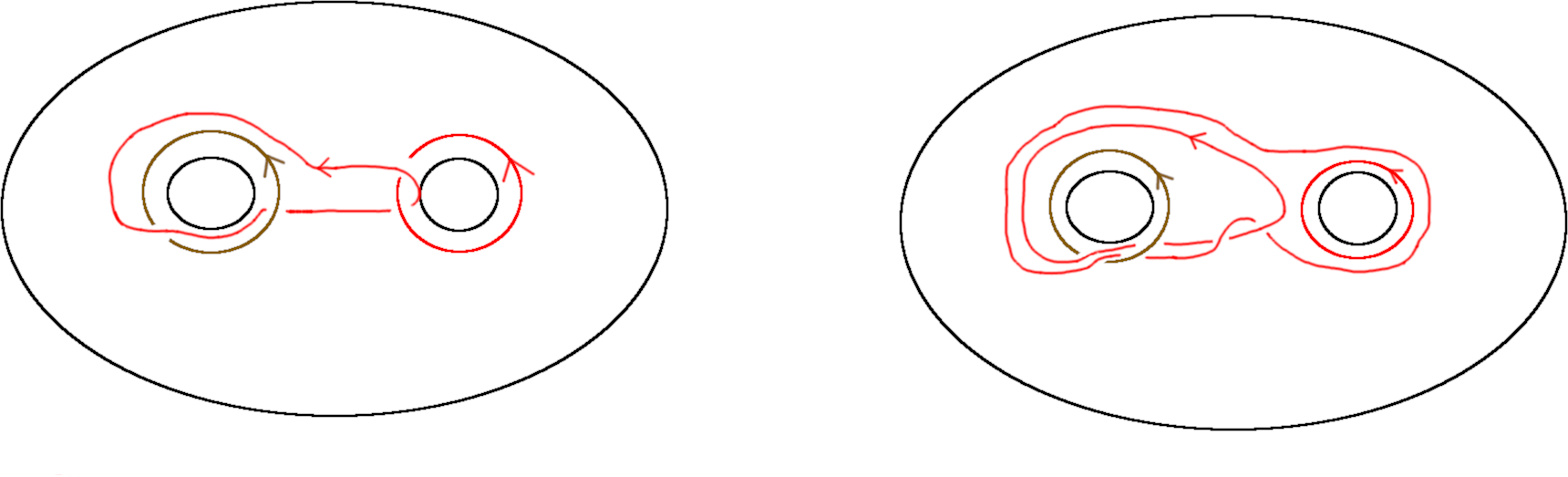
Figure 20. The links of Equation 10. The $e_{0}$ terms are drawn in brown.

Figure 21. At the top the graph $\Gamma$ obtained after one mutation of the necklace graph. Middle, the graph obtained after positively mutating at the edge of $\Gamma$ labelled $U_{2}$. Bottom, the graph obtained by mutating the middle graph at the edge labelled $U_{1}-V_{2}$ label.

Figure 22. The other path of mutations. At the top the graph obtained from $\Gamma$ by positively mutating at the edge labelled by $U_{1}-V_{2}$. The middle graph is obtained from positive mutation at the edge labelled $U_{1}+U_{2}-V_{1}$. The bottom graph is obtained by positive mutation at the edge labelled by $U_{2}$.

References

- [1] Mina Aganagic, Albrecht Klemm, Marcos Marino, and Cumrun Vafa. The topological vertex. Communications in mathematical physics, 254(2):425–478, 2005.
- [2] Anna Aiston and Hugh Morton. Idempotents of Hecke algebras of type . J. Knot Theory Ramifications, 7(4):463–487, 1998.
- [3] Denis Auroux. Mirror symmetry and T-duality in the complement of an anticanonical divisor. arXiv preprint arXiv:0706.3207, 2007.
- [4] Roger Casals and Eric Zaslow. Legendrian weaves: N-graph calculus, flag moduli and applications. arXiv:2007.04943.
- [5] Tobias Ekholm. Morse flow trees and Legendrian contact homology in 1-jet spaces. Geom. Topol., 11:1083–1224, 2007.
- [6] Tobias Ekholm. Rational symplectic field theory over Z/2 for exact Lagrangian cobordisms. J. Eur. Math. Soc.(JEMS), 10(3):641–704, 2008.
- [7] Tobias Ekholm, Ko Honda, and Tamás Kálmán. Legendrian knots and exact Lagrangian cobordisms, 2012, 1212.1519.
- [8] Tobias Ekholm and Tamás Kálmán. Isotopies of Legendrian 1-knots and Legendrian 2-tori. J. Symplectic Geom., 6(4):407–460, 2008.
- [9] Tobias Ekholm and Yanki Lekili. Duality between Lagrangian and Legendrian invariants. arXiv:1701.01284.
- [10] Tobias Ekholm and Vivek Shende. Colored HOMFLYPT counts holomorphic curves. arXiv:2101.00619.
- [11] Tobias Ekholm and Vivek Shende. Counting bare curves. in preparation.
- [12] Tobias Ekholm and Vivek Shende. Ghost bubble censorship. arXiv:2212.05835.
- [13] Tobias Ekholm and Vivek Shende. Skein recursion for holomorphic curves and invariants of the unknot. arXiv:2012.15366.
- [14] Tobias Ekholm and Vivek Shende. Skeins on branes. arXiv:1901.08027.
- [15] Yakov Eliashberg, Sheel Ganatra, and Oleg Lazarev. Flexible lagrangians. International Mathematics Research Notices, 2020(8):2408–2435, 2020.
- [16] Ludwig Faddeev and Rinat Kashaev. Quantum dilogarithm. Modern Physics Letters A, 9(05):427–434, 1994.
- [17] Ludwig Faddeev and Alexander Volkov. Abelian current algebra and the Virasoro algebra on the lattice. Physics Letters B, 315(3-4):311–318, 1993.
- [18] Vladimir Fock and Alexander Goncharov. Moduli spaces of local systems and higher Teichmüller theory. Publications Mathématiques de l’IHÉS, 103:1–211, 2006.
- [19] Vladimir Fock and Alexander Goncharov. Cluster ensembles, quantization and the dilogarithm. Annales scientifiques de l’Ecole normale supérieure, 42(6):865–930, 2009.
- [20] Sheel Ganatra, John Pardon, and Vivek Shende. Microlocal Morse theory of wrapped Fukaya categories. arXiv:1809.08807.
- [21] Sheel Ganatra, John Pardon, and Vivek Shende. Sectorial descent for wrapped Fukaya categories. arXiv:1809.03427.
- [22] Sheel Ganatra, John Pardon, and Vivek Shende. Covariantly functorial wrapped Floer theory on Liouville sectors. Publications mathématiques de l’IHÉS, 131(1):73–200, 2020.
- [23] Patrick M Gilmer and Jianyuan K Zhong. The HOMFLYPT skein module of a connected sum of 3–manifolds. Algebraic & Geometric Topology, 1(1):605–625, 2001.
- [24] Alexander Goncharov. Pentagon relation for the quantum dilogarithm and quantized . Geometry and Dynamics of Groups and Spaces: In Memory of Alexander Reznikov, pages 415–428, 2008.
- [25] Mark Gross, Paul Hacking, Sean Keel, and Maxim Kontsevich. Canonical bases for cluster algebras. Journal of the American Mathematical Society, 31(2):497–608, 2018.
- [26] Richard Hadji and Hugh Morton. A basis for the full HOMFLY skein of the annulus. Math. Proc. Cambridge Philos. Soc., 141(1):81–100, 2006.
- [27] Hirosi Ooguri and Cumrun Vafa. Knot invariants and topological strings. Nucl. Phys., B577:419–438, 2000.
- [28] James Pascaleff and Dmitry Tonkonog. The wall-crossing formula and Lagrangian mutations. Advances in Mathematics, 361:106850, 2020.
- [29] Józef Przytycki. Skein module of links in a handlebody. In Topology ’90, Ohio State University Mathematical Research Institute Publications, pages 315–342. De Gruyter, 1992.
- [30] Georgios Dimitroglou Rizell. Legendrian ambient surgery and Legendrian contact homology. Journal of Symplectic Geometry, 14(3):811–901, 2016.
- [31] Matthias Scharitzer and Vivek Shende. Quantum mirrors of cubic planar graph Legendrians. 2023, 2304.01872.
- [32] Gus Schrader, Linhui Shen, and Eric Zaslow. The chromatic Lagrangian: wavefunctions and open Gromov-Witten conjectures. arXiv:2302.00159.
- [33] Marcel-Paul Schutzenberger. Une interprétation de certaines solutions de l’équation fonctionnelle f(x+y) = f(x)f(y). C. R. Acad. Sci. Paris, 236(4):352–354, 1953.
- [34] Vivek Shende, David Treumann, and Harold Williams. On the combinatorics of exact Lagrangian surfaces. arXiv:1603.07449.
- [35] Vivek Shende, David Treumann, Harold Williams, and Eric Zaslow. Cluster varieties from Legendrian knots. Duke Mathematical Journal, 168(15):2801–2871, 2019.
- [36] Bertrand Toën and Michel Vaquié. Moduli of objects in dg-categories. In Annales scientifiques de l’Ecole normale supérieure, volume 40, pages 387–444, 2007.
- [37] David Treumann and Eric Zaslow. Cubic planar graphs and Legendrian surface theory. arXiv:1609.04892.
- [38] Edward Witten. Chern-Simons gauge theory as a string theory. Prog. Math., 133:637–678, 1995.