Identifying Klein tunneling signatures in bearded SSH lattices from bent flat bands

Abstract

Su-Schrieffer-Heeger (SSH) lattices have helped to understand key concepts of topological insulators. In this paper, we study the transmission properties of $pn$ junctions of bearded SSH lattices forming a bipartite structure. From a tight-binding approach, a Bloch Hamiltonian depicts the electron behavior as a massive pseudo-spin one particle in quasi-one-dimensional systems. It is possible to design the band structure of these lattices by tuning the on-site energy and hopping parameters. The characteristic flat band of pseudo-spin one systems can be bent by the staggered potential of the bottom atom in the bearded edge. We explore interband transmissions from the bent flat band to the valence one of a bipartite structure, where Klein tunneling can be obtained depending on the hopping parameter associated with the bearded edge. The identification of Klein tunneling signatures is feasible in artificial lattices such as photonic lattices, elastic resonators, topolectric circuits, or quantum dot arrangements. On the other hand, the study of Klein tunneling in polyatomic molecules may contribute to advance in one-dimensional transistors.

I Introduction

Klein tunneling is one of the most outstanding transport effects with experimental realizations in graphene and artificial systems Katsnelson2006 ; Allain2011 ; Beenakker2008 ; CastroNeto2009 ; Young2009 ; Jiang2020 . This effect consists of the perfect crossing of a particle within the electrostatic potential profile, where kinetic energies can be less than the barrier potential height Klein1929 ; Katsnelson2006 ; Beenakker2008 ; CastroNeto2009 . Since 1929, Oskar Klein predicted this tunneling in the context of high-energy physics without testing so far Klein1929 . In condensed matter, Klein tunneling emerges when electrons pass from one band to another with the conservation of an associated pseudo-spin lattice Katsnelson2006 . From the experimental realization of Klein tunneling in graphene Young2009 , multiple proposals of related phenomena have been predicted with some tests in artificial lattices Jiang2020 ; Zhang2022c ; Zhu2023 . On this recent topic is remarkable the prediction of super-Klein tunneling of electrons in two-dimensional lattices with unit cells containing three atoms, among them: dice lattices, Lieb lattices, and honeycomb superlattices Bercioux2009 ; Shen2010 ; Dora2011 ; Lan2011 ; Urban2011 ; Xu2016 ; Bercioux2017 ; BetancurOcampo2017 ; ContrerasAstorga2020 ; Cunha2020 ; Chen2019 ; Wang2020 ; Hao2021 ; Liu2022 ; Kim2019 ; Wang2022 ; Liu2023 ; Duan2023 ; Kim2019a ; BetancurOcampo2018 ; Jakubsky2023 ; Zeng2022 ; Korol2018 ; CrastodeLima2020 ; Nandy2019 ; Kim2020 ; Filusch2020 . In such systems, electrons behave as particles with pseudo-spin one, where a flat band lies between two dispersive bands Bercioux2017 . The study of materials with flat bands has increased recently due to its outstanding effects on electronic properties Wang2021 ; Zhang2022 ; Wang2021a ; Wang2020a ; Li2022 ; Zhang2022a ; Zhang2022b ; Wen2023 ; BetancurOcampo2017a ; NavarroLabastida2023 . Super-Klein tunneling has a recent experimental realization in phononic crystals Zhu2023 . Also, anomalous Klein tunneling, which is a non-resonant perfect transmission angularly dependent, appears for borophene 8-pmmn and uniaxially strained graphene Xie2019 ; BetancurOcampo2018 ; Huang2023 ; Xu2023 . This phenomenon has experimental observation in photonic graphene Zhang2022c . In Kekulé graphene superlattices, other type of Klein tunneling is predicted, where perfect transmission goes along with a valley-flip Garcia2022 . Anti-Klein tunneling, which is perfect back-scattering under normal incidence, and its omnidirectional perfect reflection named anti-super-Klein tunneling, have been studied in 2D materials such as bilayer graphene and phosphorene Katsnelson2006 ; BetancurOcampo2019 ; BetancurOcampo2020 ; Majari2023 ; Septembre2023 ; Cunha2020 ; MolinaValdovinos2022 . Beyond the Klein tunneling, more phenomena with flat bands have been predicted, such as Andreev reflection Beenakker2008 ; Feng2020 ; Zeng2022 ; Septembre2023 , topological charge pump Wang2021 , super skew scattering Wang2021a , Seebeck and Nernst effects Duan2023 , enhanced magneto-optical effect Chen2019 , Anderson localization Kim2019 , and electron-beam collimation Wang2022 ; Xu2016 .

Recently, there has been a remarkable increment of research related to one-dimensional lattices, particularly in artificial systems, where toy models based on the tight-binding approach are developed CaceresAravena2022 ; Coutant2021 ; Dietz2018 ; Torrent2013 ; MartinezArgueello2022 ; Stegmann2017 ; RamirezRamirez2020 ; Casteels2016 ; Majari2021 ; Belopolski2017 ; Torrent2013 ; Freeney2022 ; RamirezRamirez2020 ; Dietz2018 ; MartinezArgueello2022 ; Liu2022 ; Suesstrunk2015 ; Bellec2013 ; Drost2017 . Most of these investigations focus on the study of topological insulators Hasan2010 ; Asboth2016 ; Shen2017 . Photonic CaceresAravena2022 , phononic Coutant2021 ; Wang2020b ; Li2018 ; Kim2020 ; Tang2022 , elastic wires Thatcher2022 , water waves Yang2016 , atomic arrangements Meier2016 , and quantum dots lattices Kiczynski2022 serve to emulate 1D chains of polyacetylene, veryfing topological states predicted by the Su-Schrieffer-Heeger (SSH) model Su1979 ; Heeger1988 . This model gives the most simple description of topological insulators, where outstanding effects have been studied, among them the formation of solitons Su1979 and the conductivity in polymers Heeger1988 ; Paasch1992 . Multiple extensions of the SSH model have been proposed Li2022a ; Xie2019 ; Ahmadi2020 ; Kim2020 ; Lieu2018 ; Li2014 ; Manda2023 , which depicts unusual physical properties such as non-hermitian skin effect Liu2022 , Dirac states Li2022 , doublons Azcona2021 , and gap solitons Tang2022 . Likewise, the emergence of flat bands is not exclusive to higher dimensional lattices but also in one-dimensional chains, where localized states are observed Hao2023 ; Maimaiti2017 ; Huda2020 ; Catarina2022 ; Liu2013 ; Tilleke2020 ; Mukherjee2015 .

Nevertheless, Klein tunneling has been explored scarcely in 1D chains. It could be due to the difficulty of creating an abrupt $pn$ junction in polyacetylene and other molecules to test perfect tunneling. However, the rise of artificial lattices allows us to export unusual phenomena from condensed matter towards optics, acoustics, elastic waves, or another field Freeney2022 . Therefore, toy models based on a tight-binding approach may go beyond academic curiosity due to the universality of the Bloch theorem.

In this paper, we look for the parameters regime to obtain Klein tunneling in bearded SSH lattices. SSH chains are modified by adding extra bonds to create a bearded edge, as shown in Fig. 1. The developed tight-binding model to nearest neighbors is applied to the three lattices shown in Fig. 1. The main advantage for considering bearded edge is that excitations possess pseudo-spin one to the difference of the conventional SSH chains, where the electrons or quasi-particles have pseudo-spin 1/2. The most general situation to analyze the effects on the band structure is to take the three on-site energies and the hopping parameters of the unit cell differently. We establish the condition for creating a flat band in bearded SSH lattices. We analyze the bending effect in the flat band on the transmission in bipartite bearded SSH lattices to identify Klein tunneling signatures. Possible experimental setups to test the present results may be the implementation of elastic resonators, photonic chains, topolectric circuits, or quantum dot arrangements Freeney2022 .

II Tight binding approach of bearded SSH lattices

Bearded-SSH lattices are chains that possess a part identical to those described by the SSH model and a bearded edge whose unit cell has three atoms, as shown in Fig. 1. Geometrically, these lattices can be different by changing the angle $\alpha$ in the zigzag bond. However, bearded SSH lattices are topologically identical because it is always possible to define the lattice constant as $a=2a_{0}\cos\alpha$, where $a_{0}$ is the bond length and $\alpha$ is the bond angle for the zigzag edge. The tuning of $\alpha$ causes expansion of the band structure only with respect to the case $\alpha=0$. We can consider three atomic positions within the unit cell with different on-site energies. In the tight-binding approach, we take into account the nearest-neighbor interactions only. The on-site energies in Fig. 1 are $\epsilon_{1}$, $\epsilon_{2}$, and $\epsilon_{3}$ for the atoms in blue, green, and red color, respectively. While hopping parameters $h$, $t$, and $t^{\prime}$ describe the interaction to nearest neighbors between red-blue, blue-green, and green-blue atoms, respectively.

With these considerations, the Bloch Hamiltonian of the bearded-SSH lattice can be represented by a $3\times 3$ matrix given by (see appendix)

$$H(k)=\left(\begin{array}[]{ccc}\epsilon_{1}&g^{*}(k)&h\\ g(k)&\epsilon_{2}&0\\ h&0&\epsilon_{3}\end{array}\right),$$ (1)

where $k$ is the wave vector and $g(k)=t\exp(-ika/2)+t^{\prime}\exp(ika/2)$. This Hamiltonian is similar to the Hamiltonian of the SSH model. Diagonalizing this Hamiltonian, we obtain three bands as a function of $k$. A conventional SSH model has two energy bands. The hopping parameter $h$ modulates the properties of the SSH chain with the introduction of an extra energy band, as shown in Fig. 2. While the on-site energy $\epsilon_{3}$ controls the bending of the middle band by offering a grade of freedom for the transmission.

(a)

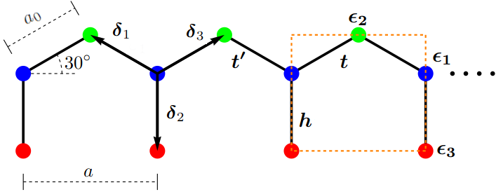
(b)

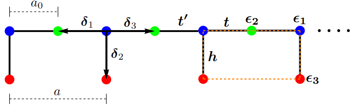
(c)

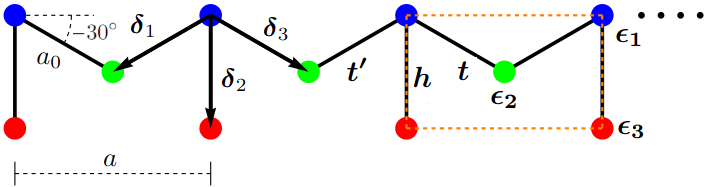
Figure 1: Different geometries for the bearded Su-Schrieffer-Heeger (SSH) lattices. The atoms are indicated by colored circles and nearest bonds with black lines. The unit cell, which is drawn by a dashed orange rectangle, has a length of $a=2a_{0}\cos\alpha$, and the relative atomic positions are given by $\boldsymbol{\delta}_{1}=a_{0}(-\cos\alpha,\sin\alpha)$, $\boldsymbol{\delta}_{2}=-a_{0}(0,1)$, and $\boldsymbol{\delta}_{3}=a_{0}(\cos\alpha,\sin\alpha)$. Examples of bearded SSH lattices are the bearded edge of a zigzag graphene nanoribbon, where $\alpha=30^{\circ}$ in (a), the edge of a Lieb nanoribbon with $\alpha=0^{\circ}$ in (b), while negative values of $\alpha$ can be considered, as shown in (c) with $\alpha=-30^{\circ}$.

One can relate the Hamiltonian in Eq. (1) with the spin-one matrices. This relation shows the behavior of the electrons like quasi-particles of pseudospin equal to one, as follows

$$H(k)=2\boldsymbol{S}\cdot\boldsymbol{g}(k)+M,$$ (2)

where $\boldsymbol{S}=(S_{x},S_{y})$ are the spin one matrices given by

$$S_{x}=\frac{1}{2}\left(\begin{array}[]{ccc}0&1&0\\ 1&0&0\\ 0&0&0\end{array}\right) S_{y}=\frac{1}{2}\left(\begin{array}[]{ccc}0&-i&0\\ i&0&0\\ 0&0&0\end{array}\right),$$ and (9)

$\boldsymbol{g}(k)=(\textrm{Re}\{g(k)\},\textrm{Im}\{g(k)\})$, and $M$ is defined as a matrix responsible of the gap opening

$$M=\left(\begin{array}[]{ccc}\epsilon_{1}&0&h\\ 0&\epsilon_{2}&0\\ h&0&\epsilon_{3}\end{array}\right).$$ (10)

(a)	(b)	(c)

Figure 2: (a) Band structure of the bearded SSH lattice. The colored curves correspond to different values of the hopping parameter $h$, where on-site energies are $\epsilon_{i}=0$, with $i=1,2$, and 3, and the hopping parameters of the SSH model are $t=t^{\prime}=1$. The flat band remains unaffected by the change of $h$. (b) If we set the parameters $h=t=1$ and $t^{\prime}=0.5,1,$ and $1.5$, the curvature of the dispersive bands is tuned only with a constant flat band. (c) In the case $h=t=t^{\prime}=1$, $\epsilon_{1}=\epsilon_{2}=0$, and by modifying the on-site energy $\epsilon_{3}=-0.5,0,$ and 0.5, the middle band lets to be flat when $\epsilon_{2}\neq\epsilon_{3}$.

Exact analytical expressions for the eigenenergies of the Hamiltonian in Eq. (1) are obtained by setting the on-site energy $\epsilon_{2}=\epsilon_{3}$, and without loss of generality, doing $\epsilon_{1}=-\epsilon_{2}=\epsilon$. These eigenenergies are

$$E_{0}=-\epsilon\qquad\textrm{and}\qquad E_{s}=s\sqrt{\epsilon^{2}+h^{2}+|g(k)|^{2}},$$ (11)

where $s=\pm 1$ is the band index for the dispersive bands $E_{s}$ and $E_{0}$ is the energy for the flat band. The condition $\epsilon_{2}=\epsilon_{3}$ gives always a flat band. Without this condition, the flat band becomes a heavy band, whose curvature is controlled by the hopping parameter $\epsilon_{3}$.

It is possible to engineer the band structure by modifying the on-site energies $\epsilon_{j}$ with $j=1,2$, and $3$, as well as the hopping parameters $t$, $t^{\prime}$, and $h$, see Fig. 2. This modulation of the parameters can be performed through artificial systems straightforwardly, among them photonic and phononic lattices Zhang2022c ; Zhu2023 . Waveguides and elastic resonators in these lattices play the role of artificial atoms, while evanescent coupling mimics bonds among sites MartinezArgueello2022 .

In the continuum approximation, we expand the Hamiltonian in Eq. (2) around the symmetry point $K=\frac{\pi}{a}$. With the definition $k=q+K$ and considering linear terms in $q$, we obtain

$$H(q)=\hbar v_{F}S_{x}q+\tilde{M},$$ (12)

where the matrix $\tilde{M}$ is defined by

$$\tilde{M}=\left(\begin{array}[]{ccc}\epsilon_{1}&i(t^{\prime}-t)&h\\ -i(t^{\prime}-t)&\epsilon_{2}&0\\ h&0&\epsilon_{3}\end{array}\right)$$ (13)

with Fermi velocity $v_{F}=a(t+t^{\prime})/(2\hbar)$.

If we consider a position-dependent staggered potential $V(x)$ in the bearded SSH lattice, it is necessary to establish the continuity conditions of the wave function in the interface. For instance, the case of a bipartite chain with a step potential and interface located at $x=0$. To find this matching condition, we integrate the differential equation given by

$$\lim_{\epsilon\rightarrow 0}\int\limits^{\epsilon}_{-\epsilon}[H(q)+V(x)]\boldsymbol{\Psi}(x)dx = E\lim_{\epsilon\rightarrow 0}\int\limits^{\epsilon}_{-\epsilon}\boldsymbol{\Psi}(x)dx$$ (14)

$$\lim_{\epsilon\rightarrow 0}\int\limits^{\epsilon}_{-\epsilon}\left(\begin{array}[]{ccc}\epsilon_{1}+V(x)&-i\hbar v_{F}\frac{d}{dx}+i(t^{\prime}-t)&h\\ -i\hbar v_{F}\frac{d}{dx}-i(t^{\prime}-t)&\epsilon_{2}+V(x)&0\\ h&0&\epsilon_{3}+V(x)\end{array}\right)\left(\begin{array}[]{c}\psi_{1}(x)\\ \psi_{2}(x)\\ \psi_{3}(x)\end{array}\right)dx = E\lim_{\epsilon\rightarrow 0}\int\limits^{\epsilon}_{-\epsilon}\left(\begin{array}[]{c}\psi_{1}(x)\\ \psi_{2}(x)\\ \psi_{3}(x)\end{array}\right)dx.$$ (24)

We assume that there are no singularities for the potential and the wave function. In this way, it is only possible to establish the continuity of two components $\psi_{1}(x)$ and $\psi_{2}(x)$ because the third component $\psi_{3}(x)$ does not have continuity necessarily.

III Transmission in bearded SSH lattice junctions

(a)

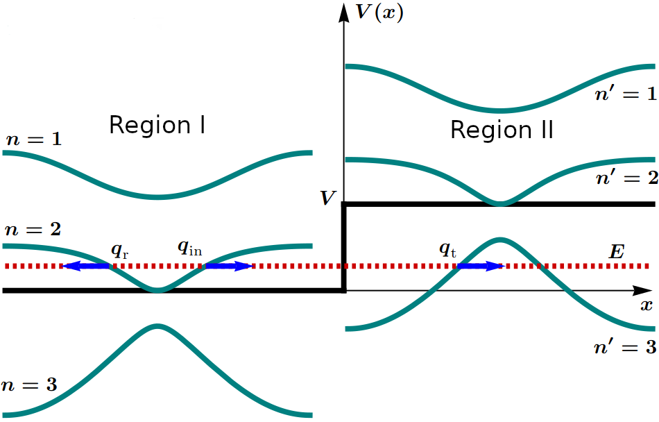
(b)

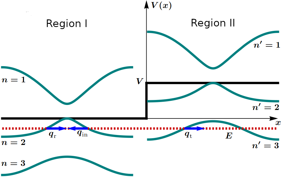
Figure 3: Electronic band structure of a $pn$ junction (green curves) based on bearded SSH lattice. This bipartite lattice emerges by applying different potentials in regions I and II. The blue arrows represent the wave vectors $q_{\textrm{in}}$, $q_{\textrm{r}}$, and $q_{\textrm{t}}$ in the electron scattering. (a) Energy bands with $\epsilon_{1}=\epsilon_{2}=0$, $\epsilon_{3}=0.5$, $t=t^{\prime}=1$, and $V=1$. The Fermi level $E$, which is indicated by the dashed red line, shows the interband transmission of electrons from the middle band in region I to the valence band in region II. (b) Same as in (a), but $\epsilon_{3}=-0.5$, the flat band is bent for obtaining negative curvature in the center.

We propose a bipartite bearded SSH lattice that consists of two coupled semi-infinity bearded SSH chains, which are modeled by a step potential. The regions I ($x<0$) and II ($x\geq 0$) have the electrostatic potential 0 and $V$, respectively. The wavefunctions for both regions are written in terms of the eigenvectors of Hamiltonian in Eq. (1)

$$\boldsymbol{\Psi}_{\textrm{I}}(x)=\boldsymbol{u}(q_{\textrm{in}})\textrm{e}^{iq_{\textrm{in}}x}+{A_{\textrm{r}}}\boldsymbol{u}(q_{\textrm{r}})\textrm{e}^{iq_{\textrm{r}}x},$$ (25)

for the region I and

$$\boldsymbol{\Psi}_{\textrm{II}}(x)=A_{\textrm{t}}\boldsymbol{u}(q_{\textrm{t}})\textrm{e}^{iq_{\textrm{t}}x}$$ (26)

is the transmitted wavefunction in region II. The quantities $A_{\textrm{r}}$ and $A_{\textrm{t}}$ are the wave amplitudes, while $q_{\textrm{r}}$ and $q_{\textrm{t}}$ are the wave vectors. We evaluate the wave vector $q_{\textrm{in}}$ as well as $q_{\textrm{r}}$ and $q_{\textrm{t}}$ in the eigenvector $\boldsymbol{u}(q_{\textrm{in}/\textrm{r}/\textrm{t}})$ according to the schematic representation of the electron scattering in the bipartite bearded SSH lattice in Fig. 3. We can select interband transmission, which corresponds to the tunneling of a single electron from the band $n$ in region I to other one $n^{\prime}$ in region II. Another possibility is the intraband transmission with $n=n^{\prime}$. We define the notation $n$-$n^{\prime}$ for the transmission to indicate that the incident electron comes from the band $n$ in region I and crosses to the band $n^{\prime}$ in region II. Propagation modes occur if electrons with energy $E$ from the band $n$ cross to the band $n^{\prime}$ when there are allowed states. We note that the group velocity direction depends on the slope sign of the tangent straight to the band. With positive curvature near to $q=0$, the maximum and minimum are located at $q_{\textrm{in},\textrm{t}}a=\pm\pi$ and $q_{\textrm{in},\textrm{t}}a=0$, respectively, and group velocity is parallel to the wave vector, as shown in Fig. 3(a). The opposite case occurs for negative curvature in the center of the band, as shown in Fig. 3(b). Propagation modes emerge if electrons from the band $n$ impinging at the interface have an energy $E_{n}(q_{\textrm{in}}a)$ which lies on the overlap between the ranges $\left[\textrm{min}\{E_{n}(0),E_{n}(\pi))\},\max\{E_{n}(0),E_{n}(\pi)\}\right]$ and $\left[\min\{E_{n^{\prime}}(0),E_{n}^{\prime}(\pi)\}+V,\max\{E_{n^{\prime}}(0),E_{n^{\prime}}(\pi)\}+V\right]$.

Applying the continuity condition at $x=0$ in the first and second components of $\Psi_{\textrm{I}}(x)$ and $\Psi_{\textrm{II}}(x)$, we have the $2\times 2$ linear equation system

$$\left(\begin{array}[]{c}u^{(1)}(q_{\textrm{in}})\\ u^{(2)}(q_{\textrm{in}})\end{array}\right)+A_{\textrm{r}}\left(\begin{array}[]{c}u^{(1)}(q_{\textrm{r}})\\ u^{(2)}(q_{\textrm{r}})\end{array}\right)=A_{\textrm{t}}\left(\begin{array}[]{c}u^{(1)}(q_{\textrm{t}})\\ u^{(2)}(q_{\textrm{t}})\end{array}\right).$$ (27)

Assuming that there is no breaking of the reflection law $q_{\textrm{r}}=-q_{\textrm{in}}$, the reflection coefficient is

$$R(q_{\textrm{in}}) = |A_{\textrm{r}}|^{2}$$

$$= \left|\frac{u^{(1)}(q_{\textrm{in}})u^{(2)}(q_{\textrm{t}})-u^{(2)}(q_{\textrm{in}})u^{(1)}(q_{\textrm{t}})}{u^{(1)}(q_{\textrm{t}})u^{(2)}(-q_{\textrm{in}})-u^{(2)}(q_{\textrm{t}})u^{(1)}(-q_{\textrm{in}})}\right|^{2}.$$

and the transmission coefficient is given by

$$T(q_{\textrm{in}})=1-R(q_{\textrm{in}})$$ (29)

due to conservation of the current density $J_{x}$.

IV Results and discussion

(a)		(b)	(c)

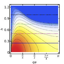
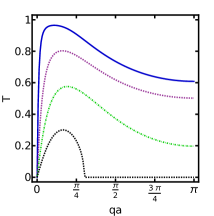
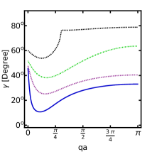
Figure 4: (a) Interband transmission from the middle band $n=2$ to valence band $n^{\prime}=3$ as a function of the hopping parameter $h$ and wave vector $q$ by using the set of values $\epsilon_{1}=\epsilon_{2}=0$, $\epsilon_{3}=0.5$, $t=t^{\prime}=1$, and potential $V=1$ (in $t$ units). Reddish region corresponds to zones with high transmission, while bluish zones indicate low transmission when energy is near a gap. (b) Interband transmission curves as a function of $q$ for the values of the hopping parameter $h=0.25,0.5,0.75$, and 1, which are depicted as blue, dashed red, dot-dashed green, and black dashed lines, respectively. These curves have their counterpart as horizontal lines in (a). (c) Relative pseudo-spin angle $\gamma$ as a function of wave vector $q$ indicating that to minimum $\gamma$, high transmission is obtained.

Our main objective is to select the interband transmissions from the bent flat band in region I towards the valence band in region II by tuning the on-site energy $\epsilon_{3}$, as shown in Fig. 3. We solve numerically Eqs. (III) and (29) taking into account that the transmitted momentum $q_{\textrm{t}}$ is determined by finding the root of $E_{n}(q_{\textrm{in}})=E_{n^{\prime}}(q_{\textrm{t}})+V$, with $n=2$ for the middle band in region I and $n^{\prime}=3$ for the valence band in region II. The relation between $q_{\textrm{in}}$ and $q_{\textrm{t}}$ is equivalent to the Snell law in quasi- one-dimensional lattices. We analyze two situations that correspond to the change of sign in the curvature of the middle band near to $q=0$, as shown in Fig. 3(a) and (b). If $\partial^{2}E_{n}/\partial q^{2}>0$ at $q=0$, wave propagation occurs from left to right for positive values of $q_{\textrm{in}}$. In the opposite case, the wave vector has to change its sign to satisfy the conservation of the current density $J_{x}$, as occurs in metamaterials.

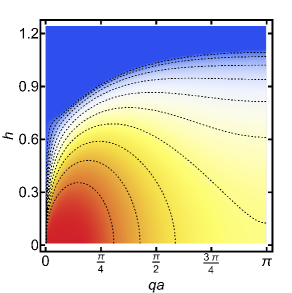
Figure 5: Same as in Fig. 4, but now $\epsilon_{3}=-0.5$. Both figures show similar features. In this case, the curvature is negative in the center of the middle band.

(a)		(b)
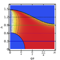
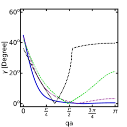
(c)		(d)

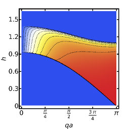
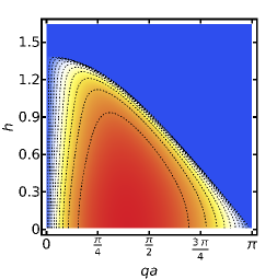
Figure 6: (a) Similar to Fig. 4 but now the transmission is from conduction band $n=1$ to valence band $n^{\prime}=3$ with potential $V=3$. Klein tunneling is predominant because the pseudo-spin of electrons in bearded SSH lattices is one. (b) Relative pseudo-spin angle as a function of $q$ shows a decay when $h$ decreases. Colors and line types for the curves correspond to the values of $h=0.3,0.6,0.9$, and $1.2$, in (a). (c) Interband transmission 1-3 with hopping parameters $t=1$ and $t^{\prime}=0.5$ favors the emergence of evanescent modes for the trivial phase in the SSH model. (d) Interband transmission with $t=1$ and $t^{\prime}=1.5$ for the topological phase.

We set the on-site energies $\epsilon_{1}=\epsilon_{2}=0$ and $\epsilon_{3}=0.5$ to bend the middle band, as seen in Fig. 3(a). We consider the interband transmission between this middle band with $n=2$ to the valence band with $n^{\prime}=3$. One can bend the band in the opposite direction by setting the value of $\epsilon_{3}=-0.5$ (see Fig. 3(b)). To analyze the effect of the hopping parameter $h$ on the transmission, we showed the transmission as a function of the momentum $q_{\textrm{in}}a\equiv qa$ and the hopping parameter $h$ in Fig. 4. To identify possible signatures of Klein tunneling, we look for areas with red color in the transmission. High transmission appear if the wave vector is within the range $0<qa<\pi/4$ and the hopping parameter in $0<h<0.3$. Particular transmission curves are shown in Fig. 4(b) for the set of values of $h=0.25,0.5$, $0.75$, and 1, noting that the transmission decreases when the hopping parameter $h$ increases. The transmission features are explained generally by using the pseudo-spin direction. In graphene, Klein tunneling emerges due to the conservation of the pseudo-spin in the normal direction Katsnelson2006 ; Young2009 . Though the system analyzed here is quasi-one-dimensional, the orientation of the pseudo-spin in the chain is represented by the polar angles $\theta$ and $\phi$ in the Bloch sphere. Since the electron scattering involves reduced components of the spinors as indicated in Eq. (27), we can relate these spinors in the Bloch sphere for the incident, reflected, and transmitted states with the set of angles $(\theta_{\textrm{in}},\phi_{\textrm{in}})$, $(\theta_{\textrm{r}},\phi_{\textrm{r}})$, and $(\theta_{\textrm{t}},\phi_{\textrm{t}})$ as a function of $q_{\textrm{in}}$. Nevertheless, our interest is to get the relative angle between the incident and transmitted state in Eq. (27). The calculation of this relative pseudo-spin angle $\gamma$ between the reduced incident and the transmitted states $\boldsymbol{w}_{i}(q_{\textrm{in}})=(u^{(1)}(q_{\textrm{in}}),u^{(2)}(q_{\textrm{in}}))$ and $\boldsymbol{w}_{t}(q_{\textrm{t}})=(u^{(1)}(q_{\textrm{t}}),u^{(2)}(q_{\textrm{t}}))$ is performed using the expression

$$\gamma=\arccos\left[\frac{|\langle w_{i}|w_{t}\rangle|}{\sqrt{\langle w_{i}|w_{i}\rangle\langle w_{t}|w_{t}\rangle}}\right].$$ (30)

It is important to note that the electrons in the bearded SSH lattice are equivalent to particles having pseudo-spin one, as seen in the Bloch Hamiltonian in Eq. (2). In pseudo-spin one systems such as $\alpha$-$\tau_{3}$ and Lieb lattices, super-Klein tunneling appears. One simple explanation of this transmission effect is that the scattering at the interface imposes the reduction of the pseudo-spin to $1/2$, as noted in Eq. (27). The relative difference in the pseudo-spin angle in Eq. (30) indicates that perfect tunneling emerges when $\gamma=0$, such as Klein tunneling in graphene Katsnelson2006 . We show this difference in the pseudo-spin direction as a function of $q$ in Fig. 4(c), where the maximum value in Fig. 4(b) corresponds to a minimum in $\gamma$. Perfect transmission occurs in $\gamma=0$, which indicates that the incident and transmitted pseudo-spin are parallel.

With negative bending of the flat band, the interband transmission 2-3 has slight modifications concerning the positive case (see Figs. 4(a) and 5 for comparison). However, the involved scattering process presents several differences. For instance, the group velocity has an opposite direction with the wave vector for both regions. Although this transmission is interband, the scattering is identical to the one intraband transmission, where the electron from the valence band in region I transits to the other valence band in region II. Similar transmission and relative pseudo-spin angles are obtained (not shown).

We analyze the interband transmission 1-3 for electrons from the conduction band to the valence band (see Fig. 6). There is a wide range for the wave vector $q$, where Klein tunneling emerges, as shown in Fig. 6(a). When $qa\rightarrow 0$, the transmission is almost zero because the energy is near the band gap. Increasing $qa$, we can observe that the transmission is perfect because the relative pseudo-spin angle $\gamma$ is zero, indicating the conservation of the pseudo-spin. The hopping parameter $h$ modulates the emergence of Klein tunneling, as shown in Fig. 6(b). Other analyses showed the robustness of the transmission by changing the on-site energy $\epsilon_{3}$, which is the parameter responsible for the bending at the middle band. We found that the change of the interband transmission 1-3 from a positive to negative curvature around the center of the band is small and similar to the one shown in Fig. 6(a). Such transmission features can be understood by the fact that the electron in the bearded SSH lattice behaves like a particle of pseudo-spin one, as described in Hamiltonian of Eq. (1), which is the quasi- one-dimensional version of the spin-orbit Hamiltonian of the Lieb lattice. The Klein tunneling observed here is robust because it is the reminiscence of the super-Klein tunneling of pseudo-spin one particles Bercioux2017 ; BetancurOcampo2017 ; ContrerasAstorga2020 .

The interband tunneling 1-3 is almost unaffected by the bending of the middle band when $t=t^{\prime}=1$. In contrast, if we set the hopping parameters $t=1$ and $t^{\prime}=0.5$ which corresponds to the trivial phase of the SSH model, the transmission changes drastically as seen in Fig. 6(c). The topological phase $t=1$ and $t^{\prime}=1.5$ presents multiple differences in transmission concerning the previous case (see Fig. 6(d)). Thus, Klein tunneling is strongly affected and sensible by tuning the hopping parameters $t$ and $t^{\prime}$. The reason is due to that $t$ and $t^{\prime}$ cause a relative shift between the band $n$ and $n^{\prime}$ still with the same step potential. Such a relative shift induces the emergence of evanescent modes, as seen in Fig. 6(c), there is a boundary that separates the regions with propagation and evanescent modes. From the case $t=t^{\prime}=1$, the relative shift of bands is negligible because the on-site energy $\epsilon_{3}$ controls the curvature of the middle band.

V Conclusions and final remarks

The bearded edge in SSH chains (see Fig. 1) modulates the band structure and transport properties through the on-site energy $\epsilon_{3}$ and hopping parameter $h$. The role of these parameters is to bend the flat band in order to explore interband tunneling. Electrons from the bent flat band in region I cross to the valence band in region II, and depending on the chosen parameters, Klein tunneling is obtained. In general, electrons in bearded SSH lattices behave like a pseudo-spin one particle and matching conditions impose the reduction of the spinors to two components in the scattering process. Klein tunneling is due to the conservation of the reduced pseudo-spin from 1 to 1/2, as pointed out in Eq. (30), Figs. 4, 5, and 6. The relative pseudo-spin angle between incident and transmitted states is not exclusive to bearded SSH lattices but also to higher dimension materials and enlarged pseudo-spin.

We analyzed interband transmissionc 1-3 from the conduction to valence band for the case $t=t^{\prime}$ by noting that the Klein tunneling is robust against the variation of the on-site energy $\epsilon_{3}$ and vertical bond parameter $h$ because this effect is the quasi-one-dimensional version of the super-Klein tunneling. However, the interband transmission 1-3 is affected strongly when $t\neq t^{\prime}$ due to the relative shift of bands. For instance, total internal reflection appears by evanescent modes. An experimental setup with $pn$ junctions of organic molecules may help to test the present results. Other platforms may be used, such as quantum dot arrangements Kiczynski2022 , photonic crystals Zhang2022c , or topolectric circuits Lee2018 ; Dong2021 ; Albooyeh2023 . In classical systems, such as elastic aluminum resonators MartinezArgueello2022 , Klein tunneling can be implemented through phonons. Emulation of $pn$ junctions can be realized by modifying the resonator size in half of the chain to obtain a bipartite bearded SSH lattice.

VI Acknowledgments

We gratefully acknowledge financial support from UNAM-PAPIIT under Project IA106223.

Appendix
General tight binding Hamiltonian of a crystal with $n$ atoms in the unit cell

The Bloch wavefunction of the electron in a crystal which satisfies the Bloch theorem is given by

$$\psi_{j}(\boldsymbol{r},\boldsymbol{k})=\sum_{\boldsymbol{R}_{\ell}}\textrm{e}^{i\boldsymbol{k}\cdot(\boldsymbol{R}_{\ell}+\boldsymbol{\delta}_{j})}\phi_{j}(\boldsymbol{r}-\boldsymbol{\delta}_{j}-\boldsymbol{R}_{\ell}),$$ (31)

where $\boldsymbol{k}$ is the wave vector, the index $j=1,2,\ldots,n$ and $\boldsymbol{R}_{\ell}$ are lattice vectors, the index $\ell$ labels the unit cell positions. The vectors $\boldsymbol{\delta}_{j}$ correspond to the atomic positions within the unit cell. The function $\phi_{j}$ is the $j$-th atomic orbital. In the following, we consider only a piece of crystal of $N$ unit cells and we suppose the expression in Eq. (31) remains valid, where $\ell$ goes from 1 to $N$.

In order to get the matrix representation of the TB Hamiltonian, we split the Hamiltonian in two parts

$$\hat{H}=\hat{H}_{\textrm{at}}+\hat{V}_{\textrm{cr}},$$ (32)

where $\hat{H}_{\textrm{at}}$ is the atomic Hamiltonian acting on the site $j$:

$$\hat{H}_{\textrm{at}}\phi_{j}(\boldsymbol{r})=\epsilon_{j}\phi_{j}(\boldsymbol{r})$$ (33)

and $\hat{V}_{\textrm{cr}}$ describes the interaction of the electron with the whole crystal. The expressions for the matrix elements are

$$H_{jm}=\int\limits_{V}\psi^{*}_{j}(\boldsymbol{r})(\hat{H}_{\textrm{at}}+\hat{V}_{\textrm{cr}})\psi_{m}(\boldsymbol{r})dV.$$ (34)

Substituting in this expression, the Bloch wave function of Eq. (31), we have

$$H_{jm}(\boldsymbol{k})=\sum_{\boldsymbol{R}^{\prime}_{\ell},\boldsymbol{R}_{\ell}}\textrm{e}^{i\boldsymbol{k}\cdot(\boldsymbol{R}_{\ell}-\boldsymbol{R}^{\prime}_{\ell}+\boldsymbol{\delta}_{m}-\boldsymbol{\delta}_{j})}\left[\epsilon_{j}W^{\ell\ell^{\prime}}_{jm}+T^{\ell\ell^{\prime}}_{jm}\right],$$ (35)

where we define

$$W^{\ell\ell^{\prime}}_{jm}(\boldsymbol{R}_{\ell})=\int\limits_{V}\phi^{*}_{j}(\boldsymbol{r}-\boldsymbol{\delta}_{j}-\boldsymbol{R}^{\prime}_{\ell})\phi_{m}(\boldsymbol{r}-\boldsymbol{\delta}_{m}-\boldsymbol{R}_{\ell})dV,$$ (36)

which is known as overlap integral because it quantifies the grade of overlapping between the orbital at the site $j$ in the unit cell $\ell$ with one located at the site $m$ within the unit cell $\ell^{\prime}$. While

$$T^{\ell\ell^{\prime}}_{jm}=\int\limits_{V}\phi^{*}_{j}(\boldsymbol{r}-\boldsymbol{\delta}_{j}-\boldsymbol{R}^{\prime}_{\ell})V_{\textrm{cr}}(\boldsymbol{r})\phi_{m}(\boldsymbol{r}-\boldsymbol{\delta}_{m}-\boldsymbol{R}_{\ell})dV$$ (37)

is the hopping integral and must be interpreted as a probability amplitude of the electron that hops from the atom $j$ in the unit cell $\ell$ to the atomic site $m$ in the unit cell $\ell^{\prime}$.

Since the vector $\Delta\boldsymbol{R}=\boldsymbol{R}_{\ell}-\boldsymbol{R}^{\prime}_{\ell}$ is also a lattice vector, there are $N$ repeated terms in Eq. (35) due to the $N$ unit cells in the crystal. Therefore, the Hamiltonian in Eq. (35) can be written as

$$H_{jm}(\boldsymbol{k})=N(\epsilon_{j}W_{jm}(\boldsymbol{k})+T_{jm}(\boldsymbol{k}))=Nh_{jm}(\boldsymbol{k}),$$ (38)

where the overlap matrix elements are

$$W_{jm}(\boldsymbol{k})=\sum_{\Delta\boldsymbol{R}}w_{jm}^{(\Delta\boldsymbol{R})}\textrm{e}^{i\boldsymbol{k}\cdot(\Delta\boldsymbol{R}+\boldsymbol{\delta}_{mj})},$$ (39)

with

$$w_{jm}^{(\Delta\boldsymbol{R})}=\int\limits_{V}\phi^{*}_{j}(\boldsymbol{r})\phi_{m}(\boldsymbol{r}-\Delta\boldsymbol{R}-\boldsymbol{\delta}_{mj})dV,$$ (40)

and the hopping matrix elements are

$$T_{jm}(\boldsymbol{k})=\sum_{\Delta\boldsymbol{R}}t_{jm}^{(\Delta\boldsymbol{R})}\textrm{e}^{i\boldsymbol{k}\cdot(\Delta\boldsymbol{R}+\boldsymbol{\delta}_{mj})},$$ (41)

where

$$t_{jm}^{(\Delta\boldsymbol{R})}=\int\limits_{V}\phi^{*}_{j}(\boldsymbol{r})V(\boldsymbol{r})\phi_{m}(\boldsymbol{r}-\Delta\boldsymbol{R}-\boldsymbol{\delta}_{mj})dV.$$ (42)

An approximation in tight-binding approach is to neglect the overlap among atoms, being $w_{jm}$ approximately the identity matrix elements.

In the case of three atoms in the unit cell, we have

$$h(\boldsymbol{k})\approx\left(\begin{array}[]{ccc}\epsilon_{1}&T_{12}(\boldsymbol{k})&T_{13}(\boldsymbol{k})\\ T_{12}^{*}(\boldsymbol{k})&\epsilon_{2}&T_{23}(\boldsymbol{k})\\ T_{13}^{*}(\boldsymbol{k})&T_{23}^{*}(\boldsymbol{k})&\epsilon_{3}\end{array}\right)$$ (43)

and considering hopping parameters to nearest neighbors

$$T_{12}(\boldsymbol{k}) \approx t_{12}\textrm{e}^{i\boldsymbol{k}\cdot\boldsymbol{\boldsymbol{\delta}}_{21}}+t^{\prime}_{12}\textrm{e}^{i\boldsymbol{k}\cdot\boldsymbol{\boldsymbol{\delta}}^{\prime}_{21}},$$ (44)

$$T_{13}(\boldsymbol{k}) \approx t_{13}\textrm{e}^{i\boldsymbol{k}\cdot\boldsymbol{\boldsymbol{\delta}}_{13}}$$ (45)

$$T_{13}(\boldsymbol{k}) \approx t_{23}\textrm{e}^{i\boldsymbol{k}\cdot\boldsymbol{\boldsymbol{\delta}}_{23}}.$$ (46)

The first expression for $T_{12}(\boldsymbol{k})$ corresponds to the interactions of the atoms at the sites 1 and 2. We show the case when the atom at the site 1 is shared once with the adjacent unit cell, where $t_{12}$ and $t^{\prime}_{12}$ are the hopping parameters. These can be different by anisotropy in the lattice. For the functions $T_{13}(\boldsymbol{k})$ and $T_{23}(\boldsymbol{k})$, we considered interactions within the unit cell only with $t_{13}$ and $t_{23}$ the nearest neighbor interactions. In the particular case of the bearded SSH lattice, we set the hopping parameters $t_{12}=t$, $t^{\prime}_{12}=t^{\prime}$, $t_{13}=h$, and $t_{23}=0$ with the relative position vectors $\boldsymbol{\delta}_{12}=a_{0}(-\cos\alpha,\sin\alpha)$, $\boldsymbol{\delta}^{\prime}_{12}=a_{0}(\cos\alpha,\sin\alpha)$, and $\boldsymbol{\delta}_{13}=-a_{0}(0,1)$, to obtain the Hamiltonian in Eq. (1).

References

- (1) M. I. Katsnelson, K. S. Novoselov, and A. K. Geim, “Chiral tunnelling and the Klein paradox in graphene,” Nature Physics 2, 620 (2006).
- (2) P. E. Allain and J. N. Fuchs, “Klein tunneling in graphene: optics with massless electrons,” The European Physical Journal B 83, 301 (2011).
- (3) C. W. J. Beenakker, “Colloquium: Andreev reflection and Klein tunneling in graphene,” Reviews of Modern Physics 80, 1337 (2008).
- (4) A. H. Castro Neto, F. Guinea, N. M. R. Peres, K. S. Novoselov, and A. K. Geim, “The electronic properties of graphene,” Reviews of Modern Physics 81, 109 (2009).
- (5) A. F. Young and P. Kim, “Quantum interference and Klein tunnelling in graphene heterojunctions,” Nature Physics 5, 222 (2009).
- (6) X. Jiang, C. Shi, Z. Li, S. Wang, Y. Wang, S. Yang, S. G. Louie, and X. Zhang, “Direct observation of Klein tunneling in phononic crystals,” Science 370, 1447 (2020).
- (7) O. Klein, “Die reflexion von elektronen an einem potentialsprung nach der relativistischen dynamik von Dirac,” Zeitschrift für Physik 53, 157 (1929).
- (8) Z. Zhang, Y. Feng, F. Li, S. Koniakhin, C. Li, F. Liu, Y. Zhang, M. Xiao, G. Malpuech, and D. Solnyshkov, “Angular-dependent Klein tunneling in photonic graphene,” Physical Review Letters 129, 233901 (2022).
- (9) Y. Zhu, A. Merkel, L. Cao, Y. Zeng, S. Wan, T. Guo, Z. Su, S. Gao, H. Zeng, H. Zhang, and B. Assouar, “Experimental observation of super-Klein tunneling in phononic crystals,” Applied Physics Letters 122, 211701 (2023).
- (10) D. Bercioux, D. F. Urban, H. Grabert, and W. Häusler, “Massless Dirac-Weyl fermions in - optical lattice” Physical Review A 80, 063603 (2009).
- (11) R. Shen, L. B. Shao, B. Wang, and D. Y. Xing, “Single Dirac cone with a flat band touching on line-centered- square optical lattices,” Physical Review B 81, 041410 (2010).
- (12) B. Dóra, J. Kailasvuori, and R. Moessner, “Lattice generalization of the Dirac equation to general spin and the role of the flat band,” Physical Review B 84, 195422 (2011).
- (13) Z. Lan, N. Goldman, A. Bermudez, W. Lu, and P. Öhberg, “Dirac-weyl fermions with arbitrary spin in two-dimensional optical superlattices,” Physical Review B 84, 165115 (2011).
- (14) D. F. Urban, D. Bercioux, M. Wimmer, and W. Häusler, “Barrier transmission of Dirac-like pseudospin-one particles,” Physical Review B 84, 115136 (2011).
- (15) H.-Y. Xu and Y.-C. Lai, “Revival resonant scattering, perfect caustics, and isotropic transport of pseudospin-1 particles,” Physical Review B 94, 165405 (2016).
- (16) D. Bercioux, O. Dutta, and E. Rico, “Solitons in one-dimensional lattices with a flat band,” Annalen der Physik 529, 1600262 (2017).
- (17) Y. Betancur-Ocampo, G. Cordourier-Maruri, V. Gupta, and R. de Coss, “Super-Klein tunneling of massive pseudospin-one particles,” Physical Review B 96, 024304 (2017).
- (18) A. Contreras-Astorga, F. Correa, and V. Jakubsky, “Super-Klein tunneling of Dirac fermions through electrostatic gratings in graphene,” Physical Review B 102, 115429 (2020).
- (19) S. M. Cunha, D. R. da Costa, L. C. Felix, A. Chaves, and J. M. Pereira, “Electronic and transport properties of anisotropic semiconductor quantum wires,” Physical Review B 102, 045427 (2020).
- (20) Y.-R. Chen, Y. Xu, J. Wang, J.-F. Liu, and Z. Ma, “Enhanced magneto-optical response due to the flat band in nanoribbons made from the - lattice,” Physical Review B 99, 045420 (2019).
- (21) J. Wang, J. F. Liu, and C. S. Ting, “Recovered minimal conductivity in the - model” Physical Review B 101, 205420 (2020).
- (22) L. Hao, “Valley-contrasting interband transitions and excitons in symmetrically biased dice model,” Physical Review B 104, 195155 (2021).
- (23) H.-L. Liu, J. Wang, and J.-F. Liu, “Electric conductivity of the line-centered honeycomb lattice,” Physica E: Low-dimensional Systems and Nanostructures 144, 115454 (2022).
- (24) S. Kim and K. Kim, “Anderson localization of two-dimensional massless pseudospin-1 Dirac particles in a correlated random one-dimensional scalar potential,” Physical Review B 100, 104201 (2019).
- (25) J. Wang and J.-F. Liu, “Super-Klein tunneling and electron-beam collimation in the honeycomb superlattice,” Physical Review B 105, 035402 (2022).
- (26) H.-L. Liu, L. Hao, J. Wang, and J.-F. Liu, “Thermopower of the dice lattice,” Physical Review B 108, 115141 (2023).
- (27) W. Duan, “Seebeck and Nernst effects of pseudospin-1 fermions in the - model under magnetic fields,” Physical Review B 108, 155428 (2023).
- (28) K. Kim, “Super-Klein tunneling of Klein-gordon particles,” Results in Physics 12, 1391 (2019).
- (29) Y. Betancur-Ocampo, “Controlling electron flow in anisotropic Dirac materials heterojunctions: a super-diverging lens,” Journal of Physics: Condensed Matter 30, 435302 (2018).
- (30) V. Jakubsky and K. Zelaya, “Lieb lattices and pseudospin-1 dynamics under barrier and well-like electrostatic interactions” Physica E: Low-dimensional Systems and Nanostructures 152, 115738 (2023).
- (31) W. Zeng and R. Shen, “Andreev reflection of massive pseudospin-1 fermions,” New Journal of Physics 24, 043021 (2022).
- (32) A. M. Korol, N. V. Medvid, and A. I. Sokolenko, “Transmission of the relativistic fermions with the pseudospin equal to one through the quasi-periodic barriers,” physica status solidi (b) 255, 9 (2018).
- (33) F. Crasto de Lima and G. J. Ferreira, “High-degeneracy points protected by site-permutation symmetries,” Physical Review B 101, 041107 (2020).
- (34) S. Nandy, K. Sengupta, and D. Sen, “Transport across junctions of pseudospin-one fermions,” Physical Review B 100, 085134 (2019).
- (35) S. Kim and K. Kim, “Omnidirectional excitation of surface waves and super-Klein tunneling at the interface between two different bi-isotropic media,” Physical Review B 101, 165428 (2020).
- (36) A. Filusch, C. Wurl, and H. Fehske, “Resonant scattering of dice quasiparticles on oscillating quantum dots,” The European Physical Journal B 93, 59 (2020).
- (37) X.-H. Wang, J. J. Wang, J. Wang, and J.-F. Liu, “Flat band assisted topological charge pump in the dice lattice,” Physical Review B 103, 195442 (2021).
- (38) Y.-C. Zhang, “Bound states in the continuum (bic) protected by self-sustained potential barriers in a flat band system,” Scientific Reports 12, 11670 (2022).
- (39) C.-Z. Wang, H.-Y. Xu, and Y.-C. Lai, “Super skew scattering in two-dimensional Dirac material systems with a flat band,” Physical Review B 103, 195439 (2021).
- (40) J. J. Wang, S. Liu, J. Wang, and J.-F. Liu, “Integer quantum hall effect of the - model with a broken flat band,” Physical Review B 102, 235414 (2020).
- (41) F. Li, Q. Zhang, and K. S. Chan, “Novel transport properties of the - lattice with uniform electric and magnetic fields,” Scientific Reports 12, 12987 (2022).
- (42) Y.-C. Zhang and G.-B. Zhu, “Infinite bound states and hydrogen atom-like energy spectrum induced by a flat band,” Journal of Physics B: Atomic, Molecular and Optical Physics 55, 065001 (2022).
- (43) Y.-C. Zhang, “Infinite bound states and 1/n energy spectrum induced by a coulomb-like potential of type iii in a flat band system,” Physica Scripta 97, 015401 (2022).
- (44) X. P. Wen and Z. P. Niu, “Highly efficient quantum heat engine operating at maximum power in the - lattice,” Physics Letters A 489, 129157 (2023).
- (45) Y. Betancur-Ocampo and V. Gupta, “Perfect transmission of 3d massive kane fermions in hgcdte veselago lenses,” Journal of Physics: Condensed Matter 30, 035501 (2017).
- (46) L. A. Navarro-Labastida and G. G. Naumis, “3/2 magic angle quantization rule of flat bands in twisted bilayer graphene and its relationship to the quantum hall effect,” Physical Review B 107, 155428 (2023).
- (47) D. Xie, W. Gou, T. Xiao, B. Gadway, and B. Yan, “Topological characterizations of an extended Su–Schrieffer–Heeger model,” npj Quantum Information 5, 55 (2019).
- (48) Y. Huang, W. Zeng, and R. Shen, “Photoinduced Klein tunneling in semi-Dirac material,” Physics Letters A 463, 128671 (2023).
- (49) Y. Xu, J. Liu, B. Xi, X. Zhou, and Y. Liu, “Pseudospin collapse, multidirectional supercollimations, and all-electrons transmission and reflection in irradiated 8-pmmn borophene,” New Journal of Physics 25, 113002 (2023).
- (50) S. G. y. García, T. Stegmann, and Y. Betancur-Ocampo, “Generalized hamiltonian for Kekulé graphene and the emergence of valley-cooperative Klein tunneling,” Physical Review B 105, 125139 (2022).
- (51) Y. Betancur-Ocampo, F. Leyvraz, and T. Stegmann, “Electron optics in phosphorene pn junctions: Negative reflection and anti-super-Klein tunneling,” Nano Letters 19, 7760 (2019).
- (52) Y. Betancur-Ocampo, E. Paredes-Rocha, and T. Stegmann, “Phosphorene pnp junctions as perfect electron waveguides,” Journal of Applied Physics 128, 114303 (2020).
- (53) P. Majari and G. G. Naumis, “Electronic Goos-Hänchen shifts in phosphorene,” Physica B: Condensed Matter 668, 415238 (2023).
- (54) I. Septembre, D. D. Solnyshkov, and G. Malpuech, “Angle-dependent Andreev reflection at an interface with a polaritonic superfluid,” Physical Review B 108, 115309 (2023).
- (55) S. Molina-Valdovinos, K. J. Lamas-Martínez, J. A. Briones-Torres, and I. Rodríguez-Vargas, “Electronic cloaking of confined states in phosphorene junctions,” Journal of Physics: Condensed Matter 34, 195301 (2022).
- (56) X. Feng, Y. Liu, Z.-M. Yu, Z. Ma, L. K. Ang, Y. S. Ang, and S. A. Yang, “Super-Andreev reflection and longitudinal shift of pseudospin-1 fermions,” Physical Review B 101, 235417 (2020).
- (57) G. Cáceres-Aravena, B. Real, D. Guzmán-Silva, A. Amo, L. E. F. F. Torres, and R. A. Vicencio, “Experimental observation of edge states in SSH-stub photonic lattices,” Physical Review Research 4, 013185 (2022).
- (58) A. Coutant, A. Sivadon, L. Zheng, V. Achilleos, O. Richoux, G. Theocharis, and V. Pagneux, “Acoustic Su–Schrieffer–Heeger lattice: Direct mapping of acoustic waveguides to the Su–Schrieffer–Heeger model,” Physical Review B 103, 224309 (2021).
- (59) B. Dietz and A. Richter, “From graphene to fullerene: experiments with microwave photonic crystals,” Physica Scripta 94, 014002 (2018).
- (60) D. Torrent, D. Mayou, and J. Sánchez-Dehesa, “Elastic analog of graphene: Dirac cones and edge states for flexural waves in thin plates,” Physical Review B 87, 115143 (2013).
- (61) A. M. Martínez-Argüello, M. P. Toledano-Marino, A. E. Terán-Juárez, E. Flores-Olmedo, G. Báez, E. Sadurní, and R. A. Méndez-Sánchez, “Molecular orbitals of an elastic artificial benzene,” Phys. Rev. A 105, 022826 (2022).
- (62) T. Stegmann, J. A. Franco-Villafañe, Y. P. Ortiz, U. Kuhl, F. Mortessagne, and T. H. Seligman, “Microwave emulations and tight-binding calculations of transport in polyacetylene,” Physics Letters A 381, 24 (2017).
- (63) F. Ramírez-Ramírez, E. Flores-Olmedo, G. Báez, E. Sadurní, and R. A. Méndez-Sánchez, “Emulating tightly bound electrons in crystalline solids using mechanical waves,” Scientific Reports 10, 10229 (2020).
- (64) W. Casteels, R. Rota, F. Storme, and C. Ciuti, “Probing photon correlations in the dark sites of geometrically frustrated cavity lattices,” Physical Review A 93, 043833 (2016).
- (65) P. Majari, E. Sadurní, M. R. Setare, J. A. Franco-Villafañe, and T. H. Seligman, “Photonic realization of the -deformed Dirac equation,” Physical Review A 104, 013522 (2021).
- (66) I. Belopolski, S.-Y. Xu, N. Koirala, C. Liu, G. Bian, V. N. Strocov, G. Chang, M. Neupane, N. Alidoust, D. Sanchez, H. Zheng, M. Brahlek, V. Rogalev, T. Kim, N. C. Plumb, C. Chen, F. Bertran, P. L. F‘evre, A. TalebIbrahimi, M.-C. Asensio, M. Shi, H. Lin, M. Hoesch, S. Oh, and M. Z. Hasan, “A novel artificial condensed matter lattice and a new platform for one-dimensional topological phases,” Science Advances 3, e150169 (2017).
- (67) S. E. Freeney, M. R. Slot, T. S. Gardenier, I. Swart, and D. Vanmaekelbergh, “Electronic quantum materials simulated with artificial model lattices,” ACS Nanoscience Au 2, 198 (2022).
- (68) R. Süsstrunk and S. D. Huber, “Observation of phononic helical edge states in a mechanical topological insulator,” Science 349, 47 (2015).
- (69) M. Bellec, U. Kuhl, G. Montambaux, and F. Mortessagne, “Tight-binding couplings in microwave artificial graphene,” Physical Review B 88, 115437 (2013).
- (70) R. Drost, T. Ojanen, A. Harju, and P. Liljeroth, “Topological states in engineered atomic lattices,” Nature Physics 13, 668 (2017).
- (71) M. Z. Hasan and C. L. Kane, “Colloquium: Topological insulators,” Reviews of Modern Physics 82, 3045 (2010).
- (72) J. K. Asbóth, L. Oroszlány, and A. Pályi, A Short Course on Topological Insulators. Springer International Publishing, 2016.
- (73) S.-Q. Shen, Topological Insulators. Springer Singapore, 2017.
- (74) T.-T. Wang, S. Bargiel, F. Lardet-Vieudrin, Y.-F. Wang, Y.-S. Wang, and V. Laude, “Phononic coupled-resonator waveguide micro-cavities,” Applied Sciences 10, 19 (2020).
- (75) X. Li, Y. Meng, X. Wu, S. Yan, Y. Huang, S. Wang, and W. Wen, “Su–Schrieffer–Heeger model inspired acoustic interface states and edge states,” Applied Physics Letters 113, 203501 (2018).
- (76) G.-J. Tang, X.-T. He, F.-L. Shi, J.-W. Liu, X.-D. Chen, and J.-W. Dong, “Topological photonic crystals: Physics, designs, and applications,” Laser amp Photonics Reviews 16, 2100300 (2022).
- (77) L. Thatcher, P. Fairfield, L. Merlo-Ramírez, and J. M. Merlo, “Experimental observation of topological phase transitions in a mechanical 1d-SSH model,” Physica Scripta 97, 035702 (2022).
- (78) Z. Yang, F. Gao, and B. Zhang, “Topological water wave states in a one-dimensional structure,” Scientific Reports 6, 29202 (2016).
- (79) E. J. Meier, F. A. An, and B. Gadway, “Observation of the topological soliton state in the Su–Schrieffer–Heeger model,” Nature Communications 7, 13986 (2016).
- (80) M. Kiczynski, S. K. Gorman, H. Geng, M. B. Donnelly, Y. Chung, Y. He, J. G. Keizer, and M. Y. Simmons, “Engineering topological states in atom-based semiconductor quantum dots,” Nature 606, 694 (2022).
- (81) W. P. Su, J. R. Schrieffer, and A. J. Heeger, “Solitons in polyacetylene,” Physical Review Letters 42, 1698 (1979).
- (82) A. J. Heeger, S. Kivelson, J. R. Schrieffer, and W. P. Su, “Solitons in conducting polymers,” Reviews of Modern Physics 60, 781 (1988).
- (83) G. Paasch, “Transport properties of new polyacetylene,” Synthetic Metals 51, 7 (1992).
- (84) C.-A. Li, S.-J. Choi, S.-B. Zhang, and B. Trauzettel, “Dirac states in an inclined two-dimensional Su–Schrieffer–Heeger model,” Physical Review Research 4, 023193 (2022).
- (85) N. Ahmadi, J. Abouie, and D. Baeriswyl, “Topological and nontopological features of generalized Su–Schrieffer–Heeger models,” Physical Review B 101, 195117 (2020).
- (86) S. Lieu, “Topological phases in the non-hermitian Su–Schrieffer–Heeger model,” Physical Review B 97, 045106 (2018).
- (87) L. Li, Z. Xu, and S. Chen, “Topological phases of generalized Su–Schrieffer–Heeger models,” Physical Review B 89, 085111 (2014).
- (88) B. M. Manda, V. Achilleos, O. Richoux, C. Skokos, and G. Theocharis, “Wave-packet spreading in the disordered and nonlinear Su–Schrieffer–Heeger chain,” Physical Review B 107, 184313 (2023).
- (89) P. M. Azcona and C. A. Downing, “Doublons, topology and interactions in a one-dimensional lattice,” Scientific Reports 11, 12540 (2021).
- (90) L. Hao, “One-dimensional flat bands and Dirac cones in narrow zigzag dice lattice ribbons,” Materials Science and Engineering: B 293, 116486 (2023).
- (91) W. Maimaiti, A. Andreanov, H. C. Park, O. Gendelman, and S. Flach, “Compact localized states and flat-band generators in one dimension,” Physical Review B 95, 115135 (2017).
- (92) M. N. Huda, S. Kezilebieke, and P. Liljeroth, “Designer flat bands in quasi-one-dimensional atomic lattices,” Physical Review Research 2, 043426 (2020).
- (93) G. Catarina and J. Fernández-Rossier, “Hubbard model for spin-1 Haldane chains,” Physical Review B 105, l081116 (2022).
- (94) X.-J. Liu, Z.-X. Liu, and M. Cheng, “Manipulating topological edge spins in a one-dimensional optical lattice,” Physical Review Letters 110, 076401 (2013).
- (95) S. Tilleke, M. Daumann, and T. Dahm, “Nearest neighbour particle-particle interaction in fermionic quasi one-dimensional flat band lattices,” Zeitschrift für Naturforschung A 75, 393 (2020).
- (96) S. Mukherjee and R. R. Thomson, “Observation of localized flat-band modes in a quasi-one-dimensional photonic rhombic lattice,” Optics Letters 40, 5443 (2015).
- (97) C. H. Lee, S. Imhof, C. Berger, F. Bayer, J. Brehm, L. W. Molenkamp, T. Kiessling, and R. Thomale, “Topolectrical circuits,” Communications Physics 1, 39 (2018).
- (98) J. Dong, V. Juricić, and B. Roy, “Topolectric circuits: Theory and construction,” Physical Review Research 3, 023056 (2021).
- (99) M. R. Albooyeh, A. Sadeghi, and S. M. Mohseni, “Topolectrical circuit correspondence design of polyacetylene,” Scientific Reports 13, 20847 (2023).