$p$-Laplacian Adaptation for Generative Pre-trained Vision-Language Models

Abstract

Vision-Language models (VLMs) pre-trained on large corpora have demonstrated notable success across a range of downstream tasks. In light of the rapidly increasing size of pre-trained VLMs, parameter-efficient transfer learning (PETL) has garnered attention as a viable alternative to full fine-tuning. One such approach is the adapter, which introduces a few trainable parameters into the pre-trained models while preserving the original parameters during adaptation. In this paper, we present a novel modeling framework that recasts adapter tuning after attention as a graph message passing process on attention graphs, where the projected query and value features and attention matrix constitute the node features and the graph adjacency matrix, respectively. Within this framework, tuning adapters in VLMs necessitates handling heterophilic graphs, owing to the disparity between the projected query and value space. To address this challenge, we propose a new adapter architecture, $p$-adapter, which employs $p$-Laplacian message passing in Graph Neural Networks (GNNs). Specifically, the attention weights are re-normalized based on the features, and the features are then aggregated using the calibrated attention matrix, enabling the dynamic exploitation of information with varying frequencies in the heterophilic attention graphs. We conduct extensive experiments on different pre-trained VLMs and multi-modal tasks, including visual question answering, visual entailment, and image captioning. The experimental results validate our method’s significant superiority over other PETL methods. Our code is available at https://github.com/wuhy68/p-Adapter/

Introduction

Recently, pre-trained language models (PLMs) (Devlin et al. 2018b; Brown et al. 2020; Liu et al. 2019; Clark et al. 2020; Raffel et al. 2020; Lewis et al. 2020) have demonstrated significant success within the Natural Language Processing (NLP) community. By leveraging massive amounts of unlabeled data during training, PLMs can learn highly performant and generalizable representations, leading to improvements on various downstream tasks. Similarly, researchers have successfully applied massive pre-training techniques to generative vision-language models (VLMs) (Li et al. 2022b, a; Cho et al. 2021). Using a sequence-to-sequence approach, generative VLMs can align cross-modal representations, which benefits multi-modal downstream tasks such as image captioning (Lin et al. 2014; Sidorov et al. 2020; Gurari et al. 2020), visual question answering (VQA) (Chen et al. 2020b; Goyal et al. 2017), etc.

To effectively transfer the knowledge gained by pre-trained VLMs to downstream tasks, fine-tuning (Devlin et al. 2018b; Howard and Ruder 2018) has become the de facto paradigm, whereby all parameters of the model are tuned for each downstream task. However, as model sizes continue to grow rapidly, fine-tuning is increasingly affected by the parameter-efficiency issue (Houlsby et al. 2019). To address this challenge, (Sung, Cho, and Bansal 2022b; Houlsby et al. 2019) have proposed a solution that involves the use of adapters, which are small, learnable modules that can be inserted into the transformer blocks. By only tuning the adapters added to the model for each downstream task while keeping the original pre-trained model fixed, this approach achieves high parameter-efficiency and has demonstrated promising results on various downstream tasks.

This paper introduces a novel modeling framework for adapter tuning coupled with attention. Specifically, we reformulate tuning adapters after attention to the spectral message passing process in GNNs on the attention graphs, wherein nodes and the edge weights are the projected query and value features and the attention weights, respectively. The attention graphs are bipartite, and each edge connects a feature in the projected query space and one in the projected value space. The discrepancy between the two feature spaces renders the attention graphs heterophilic graphs, in which the neighborhood nodes have distinct features (Fu, Zhao, and Bian 2022; Zhu et al. 2020; Tang et al. 2022). Within this framework, the standard adapter (Sung, Cho, and Bansal 2022b; Houlsby et al. 2019) tuning process becomes a spectral graph convolution with the adjacency matrix serving as the aggregation matrix on the attention graphs. However, this graph convolution is impractical for handling heterophilic graphs (Fu, Zhao, and Bian 2022).

To mitigate this heterophilic issue, we propose a new adapter module, $p$-adapter. Same as the vanilla adapter, $p$-adapter only has a small number of learnable parameters. What distinguishes $p$-adapter is to incorporate node features to renormalize the attention weights in pre-trained VLMs, which are further used for aggregating the features, inspired by $p$-Laplacian message passing (Fu, Zhao, and Bian 2022). (Fu, Zhao, and Bian 2022) proves that by carefully choosing a renormalization factor, this renormalization and aggregation process can dynamically exploit the high- and low-frequency information in the graphs, thus achieving significant performance on heterophilic graphs. Therefore, with the $p$-Laplacian calibrated attention weights, tuning $p$-adapters in pre-trained VLMs can effectively capture the information with different frequencies in the heterophilic bipartite attention graphs. Additionally, the renormalisation intensity depends on the renormalization factor $p$. Unlike $p$-Laplacian message passing (Fu, Zhao, and Bian 2022) with a fixed $p$, we adopt a layer-wise learnable strategy for determining $p$, thus rendering $p$-adapters more flexible to handle the attention graphs with different spectral properties.

We conduct extensive experiments to validate the effectiveness of our proposed method. Specifically, we test $p$-adapter on six benchmarks related to three vision-language tasks: visual question answering (Goyal et al. 2017; Gurari et al. 2018), visual entailment (Song et al. 2022), and image captioning (Lin et al. 2014; Sidorov et al. 2020; Gurari et al. 2020), using two generative pre-trained VLMs: BLIP (Li et al. 2022b) and mPLUG (Li et al. 2022a). Experimental results show our method’s significant superiority over other PETL methods.

Related Works

Vision-language models (VLMs). VLMs integrate the text and image features into an aligned representation space. Single-encoder models (Su et al. 2020; Li et al. 2020; Kim, Son, and Kim 2021; Li et al. 2021) train a unified cross-modal encoder using masked language/image modeling. Dual-encoder models (Radford et al. 2021; Jia et al. 2021) leverage two encoders for vision and language separately and include contrastive learning to align their representations. Encoder-decoder models(Li et al. 2022a, b; Wang et al. 2022; Alayrac et al. 2022), a.k.a. generative models, use a sequence-to-sequence approach for output, which endows VLMs with significant flexibility and paves the way for transferring to various generative downstream tasks, such as image captioning. In this work, we focus on the efficient adaptation of generative pre-trained VLMs.

Parameter-efficient transfer learning (PETL). Fine-tuning (Devlin et al. 2018b) has long been the default paradigm for transferring knowledge from pre-trained models to downstream tasks. However, the rapid increase in the size of pre-trained models has led to severe parameter-efficiency (Houlsby et al. 2019) issues for full fine-tuning. To bridge this gap, many PETL methods have been proposed (Houlsby et al. 2019; Hu et al. 2022; Li and Liang 2021). Adapter-based methods (Houlsby et al. 2019; Hu et al. 2022; Sung, Cho, and Bansal 2022a) introduce small learnable modules, called adapters, into pre-trained models and only fine-tune the inserted parameters during adaptation. Another trend for PETL is prefix-/prompt-tuning (Lester, Al-Rfou, and Constant 2021; Li and Liang 2021), which prepends several learnable token vectors to the keys and values in attention modules or to the input sequence directly. In this paper, we propose a new adapter architecture to handle the heterophily issue within our proposed modeling framework.

Graph Neural Networks (GNNs). GNNs (Kipf and Welling 2017; Wu et al. 2019; Veličković et al. 2018; Abu-El-Haija et al. 2018; Fu, Zhao, and Bian 2022) are neural networks operate on graph-structured data. Early GNNs are motivated from the spectral perspective, such as ChebNet (Defferrard, Bresson, and Vandergheynst 2016). Graph Convolution Networks (GCNs)(Kipf and Welling 2017; Wu et al. 2019) further simplify ChebNet and reveal the message-passing mechanism of modern GNNs. $p$-GNN (Fu, Zhao, and Bian 2022) proposes $p$-Laplacian graph message passing to handle heterophilic graphs. In this paper, we propose a new modeling framework for adapter tuning after attention, which reformulates it into a spectral graph message passing on the attention graphs and identifies the heterophilic issue therein.

Method

This section begins with a brief review of the preliminaries, encompassing graph message passing, adapters, and attention mechanism. We then present an approach to model adapter tuning after attention to graph message passing and unveil the heterophilic issue therein. Finally, we propose a new adapter architecture, $p$-adapter, to address this issue.

Preliminaries

Graph message passing. Let $\mathcal{G}=(\mathcal{V},\mathcal{E})$ be an undirected graph with node set $\mathcal{V}$ and edge set $\mathcal{E}$. Denote the node features $\bm{X}\in\mathbb{R}^{N\times d}$ and adjacency matrix $\bm{A}\in\mathbb{R}^{N\times N}$, where $N$ is the number of nodes, $d$ is node feature dimension, and $A_{ij}$ represents the edge weights between the $i$-th and the $j$-th node. The Laplacian matrix is defined as follows:

$$\bm{L}=\bm{D}-\bm{A},$$ (1)

where $\bm{D}$ is the degree matrix with diagonal entries $D_{ii}=\sum_{j}A_{ij}$ for $1\leq i\leq N$. To propagate the node features and exploit the graph information, the spectral graph message-passing process can be defined as:

$$\bm{X}^{\prime}=\sigma(\bm{C}\bm{X}\bm{W}),$$ (2)

where $\bm{X}^{\prime}$ is the node embeddings after propagation, $\bm{W}\in\mathbb{R}^{d\times d}$ is a learnable weight, $\sigma(\cdot)$ is a non-linear function, e.g., $\mathrm{ReLU}(\cdot)$ (Agarap 2018), and $\bm{C}$ is the aggregation matrix. The choice of $\bm{C}$ depends on the spectral properties one wishes to obtain. For instance, original GCN (Kipf and Welling 2017) adopts $\bm{C}=\bm{D}^{-1/2}(2\bm{I}-\bm{L})\bm{D}^{-1/2}$, which serves as a low-pass filter (Wu et al. 2019) on the spectral domain. To overcome the over-smoothing issue (Chien et al. 2021), (Fu, Zhao, and Bian 2022; Xu et al. 2018) propose to add residual connections to previous layers.

Adapter. (Houlsby et al. 2019; Sung, Cho, and Bansal 2022b) propose inserting adapters into pre-trained models and only tuning the added parameters for better parameter efficiency. An adapter is a small learnable module containing two matrices $\bm{W}_{\text{down}}\in\mathbb{R}^{l_{1}\times l_{2}}$, $\bm{W}_{\text{up}}\in\mathbb{R}^{l_{2}\times l_{1}}$ and a non-linear function $\sigma(\cdot)$, where $l_{1}$ and $l_{2}$ are the feature dimensions in pre-trained models and the hidden dimension in adapter (usually $l_{2}<l_{1}$). Given a feature $\bm{U}\in\mathbb{R}^{N\times l_{1}}$ in the pre-trained model, the adapter encoding process can be represented as:

$$\bm{U}^{\prime}=\sigma(\bm{U}\bm{W}_{\text{down}})\bm{W}_{\text{up}}+\bm{U}.$$ (3)

(Houlsby et al. 2019; Sung, Cho, and Bansal 2022b) place two adapters right after the attention and the feed-forward network in the transformer block, respectively.

Attention (Vaswani et al. 2017) has been the basic building block for foundation models (Li et al. 2022b; Brown et al. 2020; Wang et al. 2022). Given query $\bm{Q}\in\mathbb{R}^{N_{1}\times d_{k}}$, key $\bm{K}\in\mathbb{R}^{N_{2}\times d_{k}}$ and value $\bm{V}\in\mathbb{R}^{N_{2}\times d_{v}}$, attention aggregates the features by:

$$\mathrm{Attn}(\bm{Q},\bm{K},\bm{V})=\bm{M}\bm{V},$$ (4)

where

$$\bm{M}=\mathrm{softmax}\left(\frac{\bm{Q}\bm{K}^{\top}}{\sqrt{d_{k}}}\right)$$ (5)

represents the attention weights, $N_{1}$ and $N_{2}$ are the number of query and key/value features, respectively. Multi-head attention further transforms the query, key and value onto multiple sub-spaces and calculates attention on each of them, which can be formulated as:

$$\mathrm{MHA}(\bm{Q},\bm{K},\bm{V})=\mathrm{Concat}(\mathrm{head}_{1},\cdots,\mathrm{head}_{n})\bm{W}_{o},$$ (6)

where

$$\mathrm{head}_{i}=\mathrm{Attn}(\bm{Q}\bm{W}_{q}^{i},\bm{K}\bm{W}_{k}^{i},\bm{V}\bm{W}_{v}^{i}),$$ (7)

$\bm{W}_{o}\in\mathbb{R}^{d_{v}\times d_{v}}$, $n$ is the number of heads and $\bm{W}_{q}^{i},\bm{W}_{k}^{i}\in\mathbb{R}^{d_{k}\times\frac{d_{k}}{n}},\bm{W}_{v}^{i}\in\mathbb{R}^{d_{v}\times\frac{d_{v}}{n}}$ are the transformation matrices for the query, key and value in the $i$-th head, respectively.

Modeling Adapter as Graph Message Passing

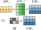
(a) Attn.

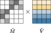
(b) Augmented Attn.

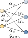
(c) Attn. graph

Figure 1: Illustration of the generation of the bipartite attention graph $\mathcal{G}_{attn}$. For simplicity, we omit the scale and softmax functions in attention mechanism.

In this section, we propose a new framework to model adapter after attention as spectral graph message passing. To simplify the notation, we consider single-head attention. From Equation 3 and Equation 4, we can formulate the features sequentially encoded by attention and adapter as:

$$\bm{U}^{\prime}=\sigma(\bm{M}\bm{V}\bm{W}_{v}\bm{W}_{o}\bm{W}_{\text{down}})\bm{W}_{\text{up}}+\bm{M}\bm{V}\bm{W}_{v}\bm{W}_{o},$$ (8)

where $\bm{M}\in\mathbb{R}^{N_{1}\times N_{2}}$ is the attention matrix computed by the transformed query $\bm{Q}\bm{W}_{q}$ and key $\bm{K}\bm{W}_{k}$ using Equation 5. The key idea of this modeling framework is to construct an attention graph, where the attention weights and features are the edge weights and node embeddings, respectively. With this attention graph, we can transform the adapter encoding process in Equation 8 into spectral graph message passing. However, direct mapping can not be applied since the adjacency matrix of an undirected graph must be square and symmetric and neither self-attention nor cross-attention satisfies this condition. For self-attention, the asymmetry arises from the distinct transform matrices of query and key spaces. For cross-attention, the attention matrix is not necessarily square if the number of query vectors does not match that of the key vectors. To bridge this gap, we consider an augmented attention mechanism. Specifically, supposing both the transformed query and value share the same dimension, we define the augmented value feature $\tilde{\bm{V}}$ which concatenates the transformed query and value and the augmented attention matrix $\tilde{\bm{M}}$ as

$$\tilde{\bm{V}}=\begin{bmatrix}\bm{Q}\bm{W}_{q}\\ \bm{V}\bm{W}_{v}\end{bmatrix},\quad\tilde{\bm{M}}=\begin{bmatrix}\bm{0}&\bm{M}\\ \bm{M}^{\top}&\bm{0}\end{bmatrix}.$$ (9)

The attention output $\bm{M}\bm{V}\bm{W}_{v}$ equals to the first $N_{1}$ features from the output of the augmented attention $\tilde{\bm{M}}\tilde{\bm{V}}$, as shown in Figure 1a and Figure 1b. Defining the projected augmented value feature $\hat{\bm{V}}=\tilde{\bm{V}}\bm{W}_{o}$, with the augmented attention mechanism, we can further define the augmented adapter encoding process by:

$$\tilde{\bm{U}}^{\prime}=\sigma(\tilde{\bm{M}}\hat{\bm{V}}\bm{W}_{\text{down}})\bm{W}_{\text{up}}+\tilde{\bm{M}}\hat{\bm{V}}.$$ (10)

Comparing Equation 8 and Equation 10, we can obtain that $\bm{U}^{\prime}=\tilde{\bm{U}}^{\prime}_{:N_{1},:}$. This indicates that the adapter encoding process and the augmented one are equal, by just taking the first $N_{1}$ elements from $\tilde{\bm{U}}^{\prime}$, thus we transform the adapter encoding process into the augmented one. Since $\tilde{\bm{M}}$ is a square and symmetric matrix, we can regard it as the adjacency matrix of the attention graph $\mathcal{G}_{attn}$, in which the nodes are features from $\hat{\bm{V}}$, i.e., $\bm{Q}\bm{W}_{q}\bm{W}_{o}$ and $\bm{V}\bm{W}_{v}\bm{W}_{o}$, and the edge weights are the corresponding attention weights computed by Equation 9. Note that during adaptation $\bm{W}_{q}$, $\bm{W}_{v}$ and $\bm{W}_{o}$ are all fixed, thus $\bm{Q}\bm{W}_{q}\bm{W}_{o}$ and $\bm{V}\bm{W}_{v}\bm{W}_{o}$ are linearly projected query and value space, respectively. Therefore, we can approximate the augmented adapter encoding process by spectral graph message passing process in Equation 2, by setting $\bm{C}=\tilde{\bm{M}}$ and $\bm{W}=\bm{W}_{\text{down}}$, considering the shortcut in adapter as a residual connection in GCN (Xu et al. 2018), and regarding $\bm{W}_{\text{up}}$ as a linear mapping after each graph convolution layer. In other words, adapter tuning can be regarded as using a one-layer GCN with the adjacency matrix serving as the aggregation matrix on $\mathcal{G}_{attn}$. Through this, we can analyze adapter tuning from a graph perspective. Upon closer inspection of $\mathcal{G}_{attn}$, we observe it to be a bipartite graph with edges connecting nodes in the projected query and value spaces, as shown in Figure 1c.

(a) Self-attention

(b) Cross-attention

Figure 2: The t-SNE (Van der Maaten and Hinton 2008) visualization of the features in the projected query and value space for self- and cross-attention. The VLM is BLIP${}_{\text{CapFilt-L}}$ (Li et al. 2022b) and data come from COCO Captions (Lin et al. 2014).

Remark 1

The attention graph $\mathcal{G}{attn}$ is a heterophilic graph in which connected nodes have dissimilar features. The visualization of the learned distribution of the projected query and value space is shown in Figure 2. We can observe that in both self- and cross-attention, the features from the two spaces differ significantly, forming two well-separated clusters. This indicates that each edge of $\mathcal{G}_{attn}$ connects two nodes from distinct feature spaces, underscoring its heterophily.

Most existing GCNs work under the homophilic assumption, which requires the labels or the features of the neighborhood nodes to be similar (Fu, Zhao, and Bian 2022; Zhu et al. 2020). When dealing with heterophilic graphs, the high-frequency information in the spectral domain will be infeasible for vanilla GCNs to exploit (Tang et al. 2022), since they mostly perform as low-pass filters (Tang et al. 2022; Wu et al. 2019; Fu, Zhao, and Bian 2022). Therefore, the heterophilic nature of $\mathcal{G}_{attn}$ poses challenges for adapters, which is previously shown to be equivalent to vanilla spectral graph message passing.

$p$-Adapter

Figure 3: $p$-Adapter architecture.

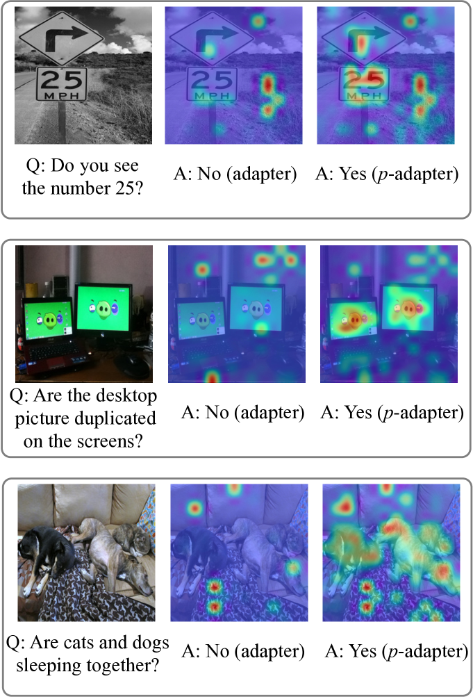
Figure 4: Attention visualization.

To tackle the heterophilic issue in adapter learning, we propose a new adapter, $p$-adapter, inspired by $p$-Laplacian message passing (Fu, Zhao, and Bian 2022).

$p$-Laplacian message passing (Fu, Zhao, and Bian 2022) is proposed for heterophilic graph learning. By denoting $\bm{\alpha}=\mathrm{diag}(\alpha_{1,1},\cdots,\alpha_{N,N})$, $\bm{\beta}=\mathrm{diag}(\beta_{1,1},\cdots,\beta_{N,N})$, and two hyper-parameters $\mu,p\in\mathbb{R}$, one-layer $p$-Laplacian message passing can be defined as:

$$\bm{X}^{\prime}=\bm{\alpha}\bm{D}^{-1/2}\bar{\bm{A}}\bm{D}^{-1/2}\bm{X}+\bm{\beta}\bm{X},$$ (11)

where $\bar{\bm{A}}$ is the $p$-Laplacian normalized adjacency matrix with entries defined by:

$$\bar{A}_{i,j}=A_{i,j}\left\|\sqrt{\frac{A_{i,j}}{D_{i,i}}}\bm{X}_{i,:}-\sqrt{\frac{A_{i,j}}{D_{j,j}}}\bm{X}_{j,:}\right\|^{p-2},$$ (12)

and for all $i,j\in[N]$ we have:

$$\alpha_{i,i}=\left(\sum^{N}_{j=1}\frac{\bar{A}_{i,j}}{D_{i,i}}+\frac{2\mu}{p}\right)^{-1},\quad\beta_{i,i}=\frac{2\mu}{p}\alpha_{i,i}.$$ (13)

The key idea of $p$-Laplacian message passing is to adopt the node features to re-normalize the adjacency matrix, as shown in Equation 12. In other words, $p$-Laplacian message passing can adaptively learn the aggregation weights for different graph-structured data. The second term in Equation 11 $\bm{\beta}\bm{X}$ is a residual term to mitigate the oversmoothing issue (Chien et al. 2021). The hyper-parameter $p$ controls the intensity of normalization, and different choices of $p$ lead to different spectral properties. When $p=2$, we impose no normalization and $p$-Laplacian message passing degenerates to vanilla GCN spectral message passing. When $p\in[1,2)$, (Fu, Zhao, and Bian 2022) proves theoretically that $p$-Laplacian message passing works as low-pass filters for nodes with small gradient, i.e., nodes with similar neighbor nodes, and works as low-high-pass filters for nodes with large gradient, i.e., nodes with dissimilar neighbor nodes. This dynamic filtering property enables $p$-Laplacian message passing to be able to handle heterophilic graphs. In (Fu, Zhao, and Bian 2022), they adopt a fixed $p$ value and test different $p$ values for different tasks. See Section A.3 for more details.

$p$-Aadapter architecture. To exploit the heterophilic attention graph $\mathcal{G}_{attn}$, the main idea of $p$-adapter is to leverage the node features to calibrate the weights of the attention/adjacency matrix, similar to $p$-Laplacian message passing (Fu, Zhao, and Bian 2022). The architecture of $p$-adapter is shown in Figure 4. The input to $p$-adapter is the intermediate result of attention. Suppose we consider the single-head case, the final output of attention should be $\bm{M}\bm{V}\bm{W}_{o}$, as shown in Equation 4 and Equation 6. For $p$-adapter, we take the attention matrix $\bm{M}$ and the projected augmented value feature $\hat{\bm{V}}$, as the output of attention. Note that this transformation does not alter any learned parameters in attention. Then, we augment the attention matrix to $\tilde{\bm{M}}$, as shown in Equation 9. Following Equation 12, we normalize the augmented attention matrix by:

$$\bar{M}_{i,j}=\tilde{M}_{i,j}\left\|\sqrt{\frac{\tilde{M}_{i,j}}{\tilde{D}_{i,i}}}\hat{\bm{V}}_{i,:}-\sqrt{\frac{\tilde{M}_{i,j}}{\tilde{D}_{j,j}}}\hat{\bm{V}}_{j,:}\right\|^{p-2},$$ (14)

where $\tilde{\bm{D}}$ is the degree matrix of $\tilde{\bm{M}}$. Then, we can obtain $\tilde{\bm{\alpha}}$ and $\tilde{\bm{\beta}}$ by replacing $\bar{\bm{A}}$ and $\bm{D}$ with $\bar{\bm{M}}$ and $\tilde{\bm{D}}$ in Equation 13, respectively. Further, we can aggregate the features using the calibrated attention matrix $\bar{\bm{M}}$ by

$$\bar{\bm{U}}=\tilde{\bm{\alpha}}\tilde{\bm{D}}^{-1/2}\bar{\bm{M}}\tilde{\bm{D}}^{-1/2}\hat{\bm{V}}+\tilde{\bm{\beta}}\hat{\bm{V}},$$ (15)

similar to Equation 11. With the aggregated feature $\bar{\bm{U}}$, we encode it with the learnable adapter weights by:

$$\bar{\bm{U}}^{\prime}=\sigma(\bar{\bm{U}}\bm{W}_{\text{down}})\bm{W}_{\text{up}}+\bar{\bm{U}}.$$ (16)

The output of $p$-adapter is $\bar{\bm{U}}^{\prime}_{:N_{1},:}$, since we only collect the features aggregated on the query nodes in the attention graph $\mathcal{G}_{attn}$. By adopting the renormalization technique inspired by $p$-Laplacian message passing (Fu, Zhao, and Bian 2022), $p$-adapter can effectively handle the heterophilic issue in $\mathcal{G}_{attn}$ and lead to improvements on various downstream tasks. Moreover, unlike (Fu, Zhao, and Bian 2022) using a fixed $p$ value, we adopt a layer-wise learnable strategy for determining value $p$. In addition, $p$-adapter is compatible with vanilla adapter (Houlsby et al. 2019; Sung, Cho, and Bansal 2022b), since $p$-adapter is designed for adaptation after attention and we leave the adapter after feed-forward networks unchanged.

Experiments

Tasks and Datasets

We conduct experiments on six benchmarks related to three vision-language downstream tasks, i.e., visual question answering (VQA), visual entailment (VE) and image captioning. For VQA, we consider it as an answer generation problem, following (Cho et al. 2021; Li et al. 2022b, 2021). We test our model on VQA2.0 (Goyal et al. 2017) with the widely-used Karpathy split (Karpathy and Fei-Fei 2015) and VizWizVQA (Gurari et al. 2018). The evaluation metric is accuracy. For VE, we follow the setting in (Song et al. 2022) and adopt SNLI-VE (Xie et al. 2019) as the evaluation benchmark, with accuracy as the metric. For image captioning, we conduct extensive experiments on three benchmarks, i,e., COCO Captions (Lin et al. 2014) with Karpathy split (Karpathy and Fei-Fei 2015), TextCaps (Sidorov et al. 2020), and VizWizCaps (Gurari et al. 2020). We adopt BLEU@4 (Papineni et al. 2002) and CIDEr (Vedantam, Lawrence Zitnick, and Parikh 2015) as the evaluation metrics, same as (Li et al. 2022b; Yang et al. 2022). Please refer to Section A.1 for more details.

Implementation Details

Our experiments are implemented in PyTorch (Paszke et al. 2019) and conducted on 8 Nvidia 3090 GPUs. We validate our method on two generative pre-trained VLMs, BLIP${}_{\text{CapFilt-L}}$ (Li et al. 2022b) and mPLUG${}_{\text{ViT-B}}$ (Li et al. 2022a). Specifically, we use the encoder of BLIP${}_{\text{CapFilt-L}}$/mPLUG${}_{\text{ViT-B}}$ to encode the image, and the decoder of BLIP${}_{\text{ViT-B}}$/mPLUG${}_{\text{ViT-B}}$ to generate the answers in an auto-regressive way. Following (Gu et al. 2022; Sung, Cho, and Bansal 2022b), we freeze the encoder and only train the decoder for new tasks. We use AdamW (Loshchilov and Hutter 2017) optimizer with a weight decay of 0.05 and apply a linear scheduler. We take random image crops of resolution $224\times 224$ as the input of the encoder, and also apply RandAugment (Cubuk et al. 2020) during the training, following (Li et al. 2022b; Sung, Cho, and Bansal 2022b). We train the model for five and two epochs for VQA and VE, and image captioning, respectively. We sweep a wide range of learning rates over $\{1\times 10^{-4},2\times 10^{-4},5\times 10^{-4},1\times 10^{-3}\}$ for PETL methods, and use $2\times 10^{-5}$ for full fine-tuning, same as (Sung, Cho, and Bansal 2022b). Please refer to LABEL:appendix:B for more details.

Comparison with transfer learning methods

Method	Updated Params	VQA2.0	VizWizVQA	SNLI_VE	COCOCaps		TextCaps		VizWizCaps
		Karpathy test	test-dev	test-P	Karpathy test		test-dev		test-dev		Avg.
	(%)	Acc.(%)	Acc.(%)	Acc.(%)	BLEU@4	CIDEr	BLEU@4	CIDEr	BLEU@4	CIDEr
BLIP${}_{\text{CapFilt-L}}$
Full fine-tuning	100.00	70.56	36.52	78.35	39.1	128.7	27.1	91.6	45.7	170.0	76.40
Prefix tuning	0.71	60.49	22.45	71.82	39.4	127.7	24.8	80.0	40.6	153.3	68.95
LoRA	0.71	66.57	33.39	77.36	38.3	128.3	24.6	82.2	41.3	154.3	71.81
Adapter	6.39	69.53	35.37	78.85	38.9	128.8	25.4	86.7	43.3	160.5	74.15
$p$-Adapter (Ours)	6.39	70.39	37.16	79.40	40.4	130.9	26.1	87.0	44.5	164.1	75.54
mPLUG${}_{\text{ViT-B}}$
Full fine-tuning	100.00	70.91	59.79	78.72	40.4	134.8	23.6	74.0	42.1	157.5	75.76
Prefix tuning	0.71	60.95	47.42	72.11	39.8	133.5	18.8	51.9	35.5	135.6	66.18
LoRA	0.71	66.67	52.49	75.29	39.4	129.4	21.0	64.4	39.5	146.0	70.46
Adapter	6.39	70.65	56.50	78.56	40.3	134.7	22.9	71.5	41.9	155.6	74.73
$p$-Adapter (Ours)	6.39	71.36	58.08	79.26	40.4	135.3	23.2	73.3	43.1	160.1	76.01

Table 1: The main results on VQA2.0 (Goyal et al. 2017), VizWizVQA (Gurari et al. 2018), SNLI_VE (Xie et al. 2019), COCOCaps (Lin et al. 2014), TextCaps (Sidorov et al. 2020) and VizWizCaps (Gurari et al. 2020) for full fine-tuning (Devlin et al. 2018b; Howard and Ruder 2018), adapter (Sung, Cho, and Bansal 2022b), prefix tuning (Li and Liang 2021), LoRA (Hu et al. 2022), and our proposed $p$-adapter. We bold the scores for full fine-tuning and the highest scores separately for approaches with PETL methods.

We compare our method with full fine-tuning and other PETL methods, i.e., adapter (Houlsby et al. 2019; Sung, Cho, and Bansal 2022b), prefix tuning (Li and Liang 2021) and LoRA (Hu et al. 2022). The results are shown in Table 1.

Comparison with full fine-tuning. In general, $p$-adapter is able to achieve comparable and even better performance than full fine-tuning on most benchmarks. Specifically, on VQA2.0 (Goyal et al. 2017), $p$-adapter outperforms full fine-tuning with mPLUG${}_{\text{ViT-B}}$ while achieving comparable performance with BLIP${}_{\text{CapFilt-L}}$. For VE task, $p$-adapter achieves improvements of 1.05% and 0.54% with BLIP${}_{\text{CapFilt-L}}$ and mPLUG${}_{\text{ViT-B}}$ on SNLI_VE (Xie et al. 2019), respectively. For image captioning, $p$-adapter surpasses full fine-tuning on COCO Captions (Lin et al. 2014). The above experimental results demonstrate the effectiveness with good parameter efficiency for $p$-adapter (only tuning 6.39% parameters).

Comparison with other PETL methods. Our proposed method, $p$-adapter, outperforms other PETL methods with both BLIP${}_{\text{CapFilt-L}}$ and mPLUG${}_{\text{ViT-B}}$. Compared with full fine-tuning, prefix tuning (Li and Liang 2021) suffers from a significant performance drop on almost all the benchmarks. With the same number of tunable parameters, LoRA (Hu et al. 2022) performs better than prefix tuning (Li and Liang 2021) on all almost all the benchmarks. Adapter (Houlsby et al. 2019; Sung, Cho, and Bansal 2022b) outperforms these two methods with two times more tunable parameters. With only several extra trainable parameters compared with adapter (Houlsby et al. 2019; Sung, Cho, and Bansal 2022b) (the learnable $p$), $p$-Adapter achieves consistent improvements (Houlsby et al. 2019; Sung, Cho, and Bansal 2022b) and significantly outperforms all the PETL methods on all the benchmarks with the two pre-trained VLMs. Especially for VizWizVQA (Gurari et al. 2018), TextCaps (Sidorov et al. 2020) and VizWizCaps (Gurari et al. 2020), $p$-Adapter surpasses vanilla adapter with a large margin. This demonstrates the effectiveness of our proposed attention re-normalization and feature aggregation mechanisms inspired $p$-Laplacian message passing (Fu, Zhao, and Bian 2022).

Ablation Studies

GNN	VQA2.0	SNLI_VE	COCOCaps		Avg.
	Acc.(%)	Acc.(%)	BLEU@4	CIDEr
GCN	69.53	78.85	38.9	128.8	79.02
APPNP	70.22	79.03	39.4	129.1	79.44
GCNII	70.13	79.12	39.7	129.7	79.66
pGNN (Ours)	70.39	79.40	40.4	130.9	80.27

Table 2: Ablation study on the graph neural networks.

Concat.	VQA2.0	SNLI_VE	COCOCaps		Avg.
	Acc.(%)	Acc.(%)	BLEU@4	CIDEr
Zero	70.02	79.17	40.2	130.3	79.92
Noise	69.90	78.99	39.9	130.1	79.72
Query (Ours)	70.39	79.40	40.4	130.9	80.27

Table 3: Ablation study on the concatenation pattern in augmented attention.

$p$ Values	VQA2.0	SNLI_VE	COCOCaps		Avg.
	Acc.(%)	Acc.(%)	BLEU@4	CIDEr
Fixed $p=\,$1.25	70.38	78.84	40.3	130.8	80.08
Fixed $p=\,$1.50	70.15	78.90	40.3	130.8	80.03
Fixed $p=\,$1.75	70.34	78.94	40.1	130.7	80.02
Learnable $p$ (Ours)	70.39	79.40	40.4	130.9	80.27

Table 4: Ablation study on learnable $p$ strategy of $p$-adapters.

Method	FFN	SA	CA	VQA2.0	SNLI_VE	COCOCaps		Avg.
				Acc. (%)	Acc. (%)	BLEU@4	CIDEr
$p$-Adapter (Imps.)	✓			68.65 (-)	78.21 (-)	38.4 (-)	128.4 (-)	78.41 (-)
	✓	✓		70.11 (+0.90)	78.96 (+0.34)	39.9 (+1.4)	130.3 (+1.8)	79.82 (+1.11)
	✓		✓	69.84 (+0.67)	79.17 (+0.57)	39.1 (+0.5)	129.4 (+0.7)	79.38 (+0.61)
	✓	✓	✓	70.39 (+0.86)	79.40 (+0.55)	40.4 (+1.5)	130.9 (+2.1)	80.27 (+1.25)

Table 5: Ablation study on different insertion positions, including FFN, self- and cross-attention. In the brackets, we show the improvements achieved by $p$-adapters over adapters. When only inserted after FFN, $p$-adapters and adapters are the same. We bold the best performance and the largest improvement for each task.

In the following section, we conduct five ablation studies to further illustrate the effectiveness of $p$-adapter. For the sake of our budgeted computation resources, all ablation studies are conducted with BLIP${}_{\text{CapFilt-L}}$ on VQA2.0 (Goyal et al. 2017), SNLI_VE (Xie et al. 2019) and COCO Captions (Lin et al. 2014).

Graph neural networks. Within our modeling framework that casts adapter tuning to graph convolution, we test different GNNs for heterophilic graphs, namely APPNP (Gasteiger, Bojchevski, and Günnemann 2019) and GCNII (Chen et al. 2020a). Note that GCN (Kipf and Welling 2017) equals to the vanilla adapter. The results are shown in Table 2. Compared with vanilla adapters, adapters with message passing in APPNP (Gasteiger, Bojchevski, and Günnemann 2019) and GCNII (Chen et al. 2020a) achieve improvements on almost all the tasks, demonstrating the necessity of handling the heterophilic issues. Moreover, our proposed $p$-adapters further surpass these two designs. The major reason of adopting $p$-Laplacian message passing (Fu, Zhao, and Bian 2022) is due to its better flexibility in handling graphs with different heterophily. (Fu, Zhao, and Bian 2022) shows that different $p$-values can lead to different spectral properties, and our proposed learnable strategy for $p$ can dynamically adjust to attention graphs with various degrees of heterophily.

Concatenation in augmented attention. In the augmented attention, we concatenate the query with the value features as the augmented value features, which are further used for re-normalization in $p$-Laplacian message passing. We test two more different ways of concatenation, i.e., padding random noise and zeros, for constructing the augmented value. The results are shown in Table 3. Concatenating the query vectors outperforms the other two alternatives, suggesting that introducing the query vectors leads to more information dipicting the attention mechanism, and thus necessitates the handing of the heterophilic attention graph.

Learnable $p$ vs. fixed $p$. We compare two different strategies for determining $p$: fixed $p$ and learnable $p$. Specifically, we test three fixed different p values {1.25, 1.5, 1.75}, and we try two learnable strategies, i.e., a unified learnable $p$ (all $p$-adapters share a $p$) and layer-wise learnable $p$. The results are shown in Table 4. According to (Fu, Zhao, and Bian 2022), different p values provide different normalization intensity, thus leading to different spectral properties suitable for handling different graphs. As we can see, for fixed $p$, different tasks favor different $p$ values, which is consistent with the findings in (Fu, Zhao, and Bian 2022). Moreover, learnable strategies achieve substantial improvements compared with different fixed $p$ values.

Insertion positions. We also test different insertion positions for adapters/$p$-adapters, including FFN, self-attention, and cross-attention. As shown in Table 5, for both adapters and $p$-adapters, more insertions (after both self-attention and cross-attention) lead to the best performance on all tasks. Moreover, the improvements from appending $p$-adapters/adapters after self/cross-attention differ in tasks. For instance, insertion after self-attention leads to more improvements for VQA2.0 (Goyal et al. 2017) while SNLI_VE (Xie et al. 2019) prefers insertion after cross-attention. Additionally, when only inserting after self-attention for VQA2.0 (Goyal et al. 2017) and cross-attention for SNLI_VE (Xie et al. 2019), $p$-adapter achieves larger improvements than full insertion, which validates $p$-adapter’s effectiveness in lower-resource scenario.

Adapter size.

(a)

(b)

Figure 5: Ablation study on the adapter size. We report the results on VQA2.0 (Goyal et al. 2017) and SNLI_VE (Xie et al. 2019).

We also verify the performance with different adapter sizes. Specifically, we vary the hidden dimension (originally set to 96) of the learnable matrices in adapters, and the results on VQA2.0 (Goyal et al. 2017) and SNLI_VE (Xie et al. 2019) are shown in Figure 5. We can observe that the advantages of $p$-adapters are further enhanced with smaller adapters. For SNLI_VE (Xie et al. 2019), $p$-adapters outperform adapters with 1.54% when tuning 1.58% parameters (the hidden dimension set to 24), and the improvement becomes 2.75% when tuning 0.79% parameters (the hidden dimension set to 12) for VQA2.0 (Goyal et al. 2017).

Visualization

To validate the effectiveness of $p$-adapter, we visualize (Chefer, Gur, and Wolf 2021) the cross-attention weights at the last transformer layer on some VQA (Goyal et al. 2017) data, as shown in Figure 4. We take the [CLS] token as the query since it represents the whole question and plot the attention weights on the image features in the key/value space. As we can see, with the normalized attention weights $\bar{\bm{M}}$, $p$-adapter can dynamically calibrate the attention weights to focus on the relevant regions in the images that adapter ignores, which further improves the performance on downstream VL tasks.

Conclusion

In this paper, we first propose a new modeling framework for adapter tuning (Houlsby et al. 2019; Sung, Cho, and Bansal 2022b) after attention modules in pre-trained VLMs. Specifically, we model it into a graph message passing process on attention graphs, where the nodes and edge weights are the projected query and value features, and the attention weights, respectively. Within this framework, we can identify the heterophilic nature of the attention graphs, posing challenges for vanilla adapter tuning (Houlsby et al. 2019; Sung, Cho, and Bansal 2022b). To mitigate this issue, we propose a new adapter architecture, $p$-adapter, appended after the attention modules. Inspired by $p$-Laplacian message passing (Fu, Zhao, and Bian 2022), $p$-adapters re-normalize the attention weights using node features and aggregate the features with the calibrated attention matrix. Extensive experimental results validate our method’s significant superiority over other PETL methods on various tasks, including VQA, VE and image captioning.

Appendix A Appendix

A.1 Vision-Language Dataset Details

We evaluate our models on six visual-language benchmarks: VQA2.0 (Goyal et al. 2017) and VizWizVQA (Gurari et al. 2018) for visual question answering (VQA), SNLI_VE (Xie et al. 2019) for visual entailment (VE), and COCOCaps (Lin et al. 2014), TextCaps (Sidorov et al. 2020), and VizWizCaps (Gurari et al. 2020) for image captioning. For VQA, instead of formulating VQA as a multi-answer classification task (Chen et al. 2020b), we consider VQA as an answer generation problem, following (Cho et al. 2021; Li et al. 2022b, 2021). For VE, following (Song et al. 2022), we first convert entailment, contradiction, and neutrality into correct, incorrect, and ambiguous as the answer list. Then, we prepend a prompt “Is it correct that” to the input text. Finally, the decoder generates the answer from the answer list. For image captioning, a prompt, “What does the image describe?”, is prepended to the input text. The statistics of each dataset are shown in Table 6. Note that we do not have the ground-truth labels for the test set of VizWizVQA (Gurari et al. 2018), VizWizCaps (Gurari et al. 2020), and TextCaps (Sidorov et al. 2020), we thus split 10% data out of the training set for hyper-parameter search and use the development set as the test set.

Dataset	Data size (images/image-text pairs)
	Train	Dev	Test
VQA2.0	113.2K/605.1K	5.0K/26.7K	5.0K/26.3K
VizWizVQA	20.5K/205.2K	4.3K/43.1K	8.0K/80.0K
SNLI_VE	29.8K/529.5K	1K/17.8K	1K/17.9K
COCOCaps	113.2K/566.8K	5.0K/5.0K	5.0K/5.0K
TextCaps	21.9K/109.7K	3.1K/3.1K	3.2K/3.2K
VizWizCaps	23.4K/117.1K	7.7K/7.7K	8.0K/8.0K

Table 6: The statistics of the datasets used in our experiments.

A.2 Implementation Details

We validate our method on two generative pre-trained vision-language models, BLIP${}_{\text{CapFilt-L}}$ (Li et al. 2022b) and mPLUG${}_{\text{ViT-B}}$ (Li et al. 2022a). BLIP${}_{\text{CapFilt-L}}$ (Li et al. 2022b) is constructed based on a multi-modal encoder-decoder architecture, and uses captioning and filtering strategy to learn from noisy image-text pairs during pre-training. Meanwhile, mPLUG${}_{\text{ViT-B}}$ (Li et al. 2022a) is a vision-language model with novel cross-modal skip-connections. Instead of fusing visual and linguistic representations at the same levels, the cross-modal skip-connections enable the fusion to occur at disparate levels.

Both BLIP${}_{\text{CapFilt-L}}$ (Li et al. 2022b) and mPLUG${}_{\text{ViT-B}}$ (Li et al. 2022a) are encoder-decoder models, which have approximately twice the number of parameters as the decoder models. In order to improve the efficiency of transfer learning, following the training process of BLIP${}_{\text{CapFilt-L}}$ (Li et al. 2022b) on image captioning tasks, we reconstruct the original framework without using text encoder, and unify vision-language understanding and generation tasks through visual question answering format (Song et al. 2022). Specifically, we use the encoder of BLIP${}_{\text{CapFilt-L}}$ (Li et al. 2022b) / mPLUG${}_{\text{ViT-B}}$ (Li et al. 2022a) to encode the images, and the decoder of BLIP${}_{\text{ViT-B}}$ (Li et al. 2022b) / mPLUG${}_{\text{ViT-B}}$ (Li et al. 2022a) to generate the answers in an auto-regressive way.

Method	lr	epoch
(A) full fine-tuning	$2\times 10^{-5}$	5
(B) prompt tuning
prompt_length=16	$1\times 10^{-3}$	5
(C) lora
$\bm{r}$=8, $\alpha$=32	$1\times 10^{-3}$	5
(D) adapter
dim={96, 48, 24, 12}	$2\times 10^{-4}$	5
(E) fixed $p$-adapter
dim={96, 48, 24, 12},
$p$={1.25, 1,5, 1,75},
$\mu$={0.1, 1, 10},	$5\times 10^{-4}$	5
(F) learnable $p$-adapter
dim={96, 48, 24, 12},
$p$={1.25, 1,5, 1,75},
$\mu$={0.1, 1, 10},	$5\times 10^{-4}$	5

Table 7: VQA2.0 (Goyal et al. 2017) and SNLI_VE (Xie et al. 2019)

Method	lr	epoch
(A) full fine-tuning	$2\times 10^{-5}$	5
(B) prompt tuning
prompt_length=16	$5\times 10^{-4}$	5
(C) lora
$\bm{r}$=8, $\alpha$=32	$5\times 10^{-4}$	5
(D) adapter
dim=96	$5\times 10^{-4}$	5
(E) fixed $p$-adapter
dim=96,
$p$={1.25, 1,5, 1,75},
$\mu$={0.1, 1, 10},	$5\times 10^{-4}$	5
(F) learnable $p$-adapter
dim=96,
$p$={1.25, 1,5, 1,75},
$\mu$={0.1, 1, 10},	$5\times 10^{-4}$	5

Table 8: VizWizVQA (Gurari et al. 2018)

Both BLIP${}_{\text{CapFilt-L}}$ (Li et al. 2022b) and mPLUG${}_{\text{ViT-B}}$ (Li et al. 2022a) adopt a BERT_base (Devlin et al. 2018a) architecture (12 layers of transformers, 12 attention heads, hidden size 768) for the decoder, and the visual transformer with ViT-B/16 (Dosovitskiy et al. 2020; Radford et al. 2021) (12 layers of transformers, 12 attention heads, hidden size 768) is used as the encoder. We use the AdamW (Loshchilov and Hutter 2017) optimizer with a weight decay of 0.05 and a linear learning rate schedule. During training, we take random image crops of resolution $224\times 224$ as input, and also apply RandAugment (Cubuk et al. 2020) to improve the generalization of vision encoders. We show the hyper-parameters that we use for tuning on the downstream vision-language tasks separately in Table 7, Table 8, and Table 9.

Method	lr	epoch
(A) full fine-tuning	$2\times 10^{-5}$	2
(B) prompt tuning
prompt_length=16	$2\times 10^{-4}$	2
(C) lora
$\bm{r}$=8, $\alpha$=32	$2\times 10^{-4}$	2
(D) adapter
dim=96	$2\times 10^{-4}$	2
(E) fixed $p$-adapter
dim={96, 48, 24, 12},
$p$={1.25, 1,5, 1,75},
$\mu$={0.1, 1, 10},	$5\times 10^{-4}$	2
(F) learnable $p$-adapter
dim={96, 48, 24, 12},
$p$={1.25, 1,5, 1,75},
$\mu$={0.1, 1, 10},	$5\times 10^{-4}$	2

Table 9: COCOCaps (Lin et al. 2014), TextCaps (Sidorov et al. 2020), and VizWizCaps (Gurari et al. 2020)

A.3 $p$-Laplacian message passing

In this section, we briefly summarize the $p$-Laplacian foundations and message passing proposed in (Fu, Zhao, and Bian 2022) and (Zhou and Schölkopf 2005). We consider an undirected graph $\mathcal{G}=(\mathcal{V},\mathcal{E})$ where $\mathcal{V}$ is the node set with cardinality $N$, $\mathcal{E}\subseteq\mathcal{V}\times\mathcal{V}$ is the edge set. Let $\mathcal{H}(V)$ be the Hilbert space of all real-valued functions defined on the node set $\mathcal{\mathcal{V}}$ endowed with the well-defined inner product $\langle f,g\rangle_{\mathcal{H}(\mathcal{V})}=\sum_{v\in\mathcal{V}}f(v)g(v)$. The Hilbert space $\mathcal{H}_{\mathcal{E}}$ is similarly defined for the edge set $\mathcal{E}$. Let $u\sim v$ denote all neighbors of $v$ for simplicity.

Definition 1 (Graph Gradient)

The graph gradient (Zhou and Schölkopf 2005) of the function $f\in\mathcal{H}(\mathcal{V})$ is a function in $\mathcal{H}(\mathcal{E})$. For any edge $e_{u,v}=[u,v]\in\mathcal{E}$, the function value of graph gradient $\nabla f$ is defined by

$$\nabla f(e_{u,v})=\sqrt{\frac{w(e_{u,v})}{d(v)}}f(v)-\sqrt{\frac{w(e_{u,v})}{d(u)}}f(u),$$ (17)

where $w(e_{u,v})$ is the weight of edge $e_{u,v}$ and $d(v)=\sum_{u\sim v}d(u)$ is the degree of $v\in\mathcal{V}$.

To establish the foundation of $p$-Laplacian, we still require the definition of graph divergence.

Definition 2 (Graph Divergence)

The graph divergence (Zhou and Schölkopf 2005) is an operator $\operatorname*{div}:\mathcal{H}(\mathcal{E})\rightarrow\mathcal{H}(\mathcal{V})$ defined by

$$\operatorname*{div}{g}(v)=\sum_{u\sim v}\sqrt{\frac{w(e_{u,v})}{d(v)}}\left(g(e_{v,u})-g(e_{u,v})\right),$$ (18)

for any $v\in\mathcal{V}$.

The definition of $p$-Laplacian can be extended to the discrete analogue given the above definitions.

Definition 3 (Graph $p$-Laplacian)

The graph $p$-Laplacian (Zhou and Schölkopf 2005; Fu, Zhao, and Bian 2022) is an operator $\Delta_{p}:\mathcal{H}(\mathcal{V})\rightarrow\mathcal{H}(\mathcal{V})$ defined by

$$\Delta_{p}{f}=-\frac{1}{2}\operatorname*{div}\left(\|\nabla f\|^{p-2}\nabla f\right),$$ (19)

for some appropriate $p\geq 1$. With the help of Definition 1 and Definition 2, we can write the $p$-Laplacian in a discrete form (Zhou and Schölkopf 2005)

$$\Delta_{p}f(v)=\frac{1}{2}\sum_{u\sim v}\left(\|\nabla_{u}f\|^{p-2}+\|\nabla_{v}f\|^{p-2}\right)\cdot\\ \frac{w(e_{u,v})}{\sqrt{d(v)}}\left(\frac{f(v)}{\sqrt{d(v)}}-\frac{f(u)}{\sqrt{d(u)}}\right),$$ (20)

where the norm of the graph gradient $\nabla f$ at vertex $v$ is defined by $\|\nabla_{v}f\|^{2}=\sum_{u\sim v}(\nabla f)^{2}(e_{u,v})$.

Note that $p$ is a hyperparameter. Specially, Equation 20 degrades into the conventional normalized graph Laplacian $\bm{I}-\bm{D}^{-\frac{1}{2}}\bm{W}\bm{D}^{-\frac{1}{2}}$ where $\bm{W}$ and $\bm{D}$ are the adjacency matrix and diagonal degree matrix, respectively. The definition of norm $\|\nabla f\|$ is slightly different in (Fu, Zhao, and Bian 2022) where they treat the power of graph norm $\|\cdot\|^{p-2}$ element-wise and re-formulate Equation 20 as

$$\Delta_{p}f(v)=\sum_{u\sim v}\|\nabla{f}(e_{u,v})\|^{p-2}\cdot\\ \frac{w(e_{u,v})}{\sqrt{d(v)}}\left(\frac{f(v)}{\sqrt{d(v)}}-\frac{f(u)}{\sqrt{d(u)}}\right).$$ (21)

Equation 21 can be easily extended to vector-valued functions $f$, where the operations are treated element-wise (Fu, Zhao, and Bian 2022).

Definition 4 (Graph Function Variation)

The variation of graph function (Fu, Zhao, and Bian 2022) $f\in\mathcal{H}(\mathcal{V})$ over the graph $\mathcal{G}=(\mathcal{V},\mathcal{E})$ is defined by

$$\mathcal{S}_{p}(f)=\frac{1}{2}\sum_{e\in\mathcal{E}}\left\|\nabla f(e)\right\|^{p},$$ (22)

where $\|\cdot\|$ is the norm defined in the function domain of $f$.

Note that the summation inside variation $\mathcal{S}_{p}(f)$ in (22) is taken over the entire edge set $\mathcal{E}$, while the $p$-Dirichlet form $\mathcal{S}_{p}(f)=\frac{1}{2}\sum_{v\in\mathcal{V}}\|\nabla_{v}f\|^{p}$ in (Zhou and Schölkopf 2005) is taken over the whole node set $\mathcal{V}$.

Given node features $\bm{X}\in\mathbb{R}^{N\times d}$ and new features $\bm{F}\in\mathbb{R}^{N\times d}$ whose $i$-th rows $\bm{X}_{i,:},\bm{F}_{i,:}$ represent corresponding feature vectors, consider function $f:\mathcal{V}\rightarrow\mathbb{R}^{d}$ such that $f(v_{i})=\bm{F}_{i,:}$ where $v_{i}\in\mathcal{V}$ is the $i$-th node of $\mathcal{G}$. For convenience, we use the graph gradient tensor $\nabla\bm{F}\in\mathbb{R}^{N\times N\times d}$ of feature matrix $\bm{F}$ to depict the graph gradient $\nabla{f}$, where

$$\nabla\bm{F}_{i,j}=\nabla{f}(e_{v_{i},v_{j}})=\sqrt{\frac{W_{i,j}}{D_{j,j}}}\bm{F}_{j,:}-\sqrt{\frac{W_{i,j}}{D_{i,i}}}\bm{F}_{i,:}.$$ (23)

Note that if edge $[v_{i},v_{j}]\notin\mathcal{E}$ indicating $W_{i,j}=0$, we naturally have $\nabla\bm{F}_{i,j}$ is a zero vector. The $p$-Laplacian regularization problem  (Fu, Zhao, and Bian 2022) is defined by

$$\min_{\bm{F}}\mathcal{L}_{p}(\bm{F}):=\mathcal{S}_{p}(\bm{F})+\mu\sum_{i=1}^{N}\|\bm{F}_{i,:}-\bm{X}_{i,:}\|_{2}^{2},$$ (24)

where $\mu>0$. Given the weight matrix $\bm{W}$, the variation $\mathcal{S}_{p}(\bm{F})=\sum_{[i,j]\in\mathcal{E}}\|\nabla\bm{F}_{i,j}\|^{p}$ is simply

$$\mathcal{S}_{p}(f)=\frac{1}{2}\sum_{i=1}^{N}\sum_{j=1}^{N}\left\|\sqrt{\frac{W_{i,j}}{D_{j,j}}}\bm{F}_{j,:}-\sqrt{\frac{W_{i,j}}{D_{i,i}}}\bm{F}_{i,:}\right\|^{p}$$ (25)

according to Equation 22, where the norm $\|\cdot\|$ in Equation 25 is a vector norm in $\mathbb{R}^{d}$.

The solution to (24) is the optimal $\bm{F}^{*}$ we desire. An iterative method to solve $\bm{F}^{*}$ for general $p\geq 1$ is proposed in (Zhou and Schölkopf 2005) and applied to graph neural networks in (Fu, Zhao, and Bian 2022) called $p$-Laplacian message passing following the iterative propagation

$$\bm{F}^{(k+1)}=\bm{\alpha}^{(k)}\bm{D}^{-\frac{1}{2}}\bm{M}^{(k)}\bm{D}^{-\frac{1}{2}}\bm{F}^{(k)}+\bm{\beta}^{(k)}\bm{X},$$ (26)

where $k$ denotes the iteration number, $\bm{F}^{(k)}$ is the feature matrix at the $k$-th iteration, $\bm{M}^{(k)}$ is the normalized adjacency matrix with entries $M_{i,j}^{(k)}=W_{i,j}\|\nabla\bm{F}_{i,j}^{(k)}\|^{p-2}$, diagonal matrices $\bm{\alpha}^{(k)}$ and $\bm{\beta}^{(k)}$ are defined by

$$\alpha_{i,i}^{(k)}=\left(\sum_{j=1}^{N}\frac{M_{i,j}^{(k)}}{D_{i,i}}+\frac{2\mu}{p}\right)^{-1},\;\;\beta_{i,i}^{(k)}=\frac{2\mu}{p}\alpha_{i,i}^{(k)}.$$ (27)

Equation 26 not only provides an iterative method to compute $\bm{F}^{*}$ but also illustrates propagation scheme in graph neural networks. The properties of $p$-Laplacian is well-studied in (Fu, Zhao, and Bian 2022):

Proposition 1 (Spectral Properties (Fu, Zhao, and Bian 2022))

Given a connected graph $\mathcal{G}=(\mathcal{V},\mathcal{E},\bm{W})$ with node embeddings $\bm{F}$ and the $p$-Laplacian $\Delta_{p}$ with its $p$-eigenvectors $\{\bm{u}^{(l)}\}_{l=0,\cdots,N-1}$ and the $p$-eigenvalues $\{\lambda^{(l)}\}_{l=0,\cdots,N-1}$. Let $g_{p}(\lambda_{i-1}):=\alpha_{i,i}\sum_{j}D_{i,i}^{-\frac{1}{2}}M_{i,j}D_{j,j}^{-\frac{1}{2}}$ for $i=1,\cdots,N$ be the filters defined on the spectral domain of $\Delta_{p}$, where $M_{i,j}=W_{i,j}\|\nabla f([v_{i},v_{j}])\|^{p-2}$, $\nabla f([v_{i},v_{j}])$ is the graph gradient of the edge between node $v_{i}$ and node $v_{j}$. $N_{i}$ denotes the number of edges connected to $v_{i}$, $N_{\min}=\min_{1\leq i\leq N}N_{i}$ and $(k,l^{*})=\operatorname*{argmax}_{j,l}\frac{|u_{j}^{(l)}|}{\sqrt{D_{l,l}}}$. Then we have

1. When $p=2$, $g_{p}(\lambda_{i-1})$ works as low-high-pass filters.

2. When $p>2$, $g_{p}(\lambda_{i-1})$ works as low-high-pass filters on node $v_{i}$ if $\|\nabla_{v_{i}}f\|\leq 2^{\frac{p-1}{p-2}}$ and low-pass filters on $v_{i}$ otherwise.

3. When $1\leq p<2$, $g_{p}(\lambda_{i-1})$ works as low-pass filters on node $v_{i}$ if $\|\nabla_{v_{i}}f\|\leq 2(2\sqrt{N_{k}})^{\frac{1}{p-2}}$ and low-high-pass filters on $v_{i}$ otherwise.

Proposition 1 provides theoretical analysis of the $p$-Laplacian message passing. It is clear that $p$-Laplacian message passing with $1\leq p<2$ can deal with heterophilic graphs effectively.

In our $p$-Adapter, we apply a one-layer $p$-Laplacian message passing with a learnable $p$. Denote the node features by $\bm{X}$. $\bm{A}$ is the adjacency matrix (following the conventional notation), $\bm{D}$ is the diagonal degree matrix and $\bar{\bm{A}}$ is the normalized adjacency matrix after the graph gradient, with entries $\bar{A}_{i,j}=A_{i,j}\|\nabla\bm{X}_{i,j}\|^{p-2}$. The $p$-Laplacian message passing in Equation 26 becomes

$$\bm{X}^{\prime}=\bm{\alpha}\bm{D}^{-\frac{1}{2}}\bar{\bm{A}}\bm{D}^{-\frac{1}{2}}\bm{X}+\bm{\beta}\bm{X},$$ (28)

where $\bm{\alpha}$ and $\bm{\beta}$ are defined similarly as Equation 27.

References

- Abu-El-Haija et al. (2018) Abu-El-Haija, S.; Perozzi, B.; Al-Rfou, R.; and Alemi, A. 2018. Watch Your Step: Learning Node Embeddings via Graph Attention. In Annual Conference on Neural Information Processing Systems (NeurIPS).
- Agarap (2018) Agarap, A. F. 2018. Deep Learning using Rectified Linear Units (ReLU). ArXiv, abs/1803.08375.
- Alayrac et al. (2022) Alayrac, J.-B.; Donahue, J.; Luc, P.; Miech, A.; Barr, I.; Hasson, Y.; Lenc, K.; Mensch, A.; Millican, K.; Reynolds, M.; et al. 2022. Flamingo: a visual language model for few-shot learning. arXiv preprint arXiv:2204.14198.
- Brown et al. (2020) Brown, T.; Mann, B.; Ryder, N.; Subbiah, M.; Kaplan, J. D.; Dhariwal, P.; Neelakantan, A.; Shyam, P.; Sastry, G.; Askell, A.; Agarwal, S.; Herbert-Voss, A.; Krueger, G.; Henighan, T.; Child, R.; Ramesh, A.; Ziegler, D.; Wu, J.; Winter, C.; Hesse, C.; Chen, M.; Sigler, E.; Litwin, M.; Gray, S.; Chess, B.; Clark, J.; Berner, C.; McCandlish, S.; Radford, A.; Sutskever, I.; and Amodei, D. 2020. Language Models are Few-Shot Learners. In Annual Conference on Neural Information Processing Systems (NeurIPS), volume 33. Curran Associates, Inc.
- Chefer, Gur, and Wolf (2021) Chefer, H.; Gur, S.; and Wolf, L. 2021. Transformer interpretability beyond attention visualization. In IEEE Conference on Computer Vision and Pattern Recognition (CVPR), 782–791.
- Chen et al. (2020a) Chen, M.; Wei, Z.; Huang, Z.; Ding, B.; and Li, Y. 2020a. Simple and deep graph convolutional networks. In ICML.
- Chen et al. (2020b) Chen, Y.-C.; Li, L.; Yu, L.; El Kholy, A.; Ahmed, F.; Gan, Z.; Cheng, Y.; and Liu, J. 2020b. Uniter: Universal image-text representation learning. In European Conference on Computer Vision (ECCV), 104–120. Springer.
- Chien et al. (2021) Chien, E.; Peng, J.; Li, P.; and Milenkovic, O. 2021. Adaptive Universal Generalized PageRank Graph Neural Network. In International Conference on Learning Representations (ICLR).
- Cho et al. (2021) Cho, J.; Lei, J.; Tan, H.; and Bansal, M. 2021. Unifying vision-and-language tasks via text generation. In International Conference on Machine Learning (ICML).
- Clark et al. (2020) Clark, K.; Luong, M.-T.; Le, Q. V.; and Manning, C. D. 2020. Electra: Pre-training text encoders as discriminators rather than generators. In International Conference on Learning Representations (ICLR).
- Cubuk et al. (2020) Cubuk, E. D.; Zoph, B.; Shlens, J.; and Le, Q. V. 2020. Randaugment: Practical automated data augmentation with a reduced search space. In IEEE Conference on Computer Vision and Pattern Recognition (CVPR), 702–703.
- Defferrard, Bresson, and Vandergheynst (2016) Defferrard, M.; Bresson, X.; and Vandergheynst, P. 2016. Convolutional neural networks on graphs with fast localized spectral filtering.
- Devlin et al. (2018a) Devlin, J.; Chang, M.-W.; Lee, K.; and Toutanova, K. 2018a. Bert: Pre-training of deep bidirectional transformers for language understanding. arXiv preprint arXiv:1810.04805.
- Devlin et al. (2018b) Devlin, J.; Chang, M.-W.; Lee, K.; and Toutanova, K. N. 2018b. BERT: Pre-training of Deep Bidirectional Transformers for Language Understanding. In Annual Conference of the North American Chapter of the Association for Computational Linguistics (NAACL).
- Dosovitskiy et al. (2020) Dosovitskiy, A.; Beyer, L.; Kolesnikov, A.; Weissenborn, D.; Zhai, X.; Unterthiner, T.; Dehghani, M.; Minderer, M.; Heigold, G.; Gelly, S.; et al. 2020. An image is worth 16x16 words: Transformers for image recognition at scale. arXiv preprint arXiv:2010.11929.
- Fu, Zhao, and Bian (2022) Fu, G.; Zhao, P.; and Bian, Y. 2022. -Laplacian Based Graph Neural Networks. In International Conference on Machine Learning (ICML).
- Gasteiger, Bojchevski, and Günnemann (2019) Gasteiger, J.; Bojchevski, A.; and Günnemann, S. 2019. Predict then propagate: Graph neural networks meet personalized pagerank. In ICLR.
- Goyal et al. (2017) Goyal, Y.; Khot, T.; Summers-Stay, D.; Batra, D.; and Parikh, D. 2017. Making the v in vqa matter: Elevating the role of image understanding in visual question answering. In IEEE Conference on Computer Vision and Pattern Recognition (CVPR), 6904–6913.
- Gu et al. (2022) Gu, J.; Meng, X.; Lu, G.; Hou, L.; Niu, M.; Xu, H.; Liang, X.; Zhang, W.; Jiang, X.; and Xu, C. 2022. Wukong: 100 million large-scale chinese cross-modal pre-training dataset and a foundation framework. arXiv preprint arXiv:2202.06767.
- Gurari et al. (2018) Gurari, D.; Li, Q.; Stangl, A. J.; Guo, A.; Lin, C.; Grauman, K.; Luo, J.; and Bigham, J. P. 2018. Vizwiz grand challenge: Answering visual questions from blind people. In IEEE Conference on Computer Vision and Pattern Recognition (CVPR), 3608–3617.
- Gurari et al. (2020) Gurari, D.; Zhao, Y.; Zhang, M.; and Bhattacharya, N. 2020. Captioning images taken by people who are blind. In European Conference on Computer Vision (ECCV), 417–434. Springer.
- Houlsby et al. (2019) Houlsby, N.; Giurgiu, A.; Jastrzebski, S.; Morrone, B.; De Laroussilhe, Q.; Gesmundo, A.; Attariyan, M.; and Gelly, S. 2019. Parameter-efficient transfer learning for NLP. In International Conference on Machine Learning (ICML). PMLR.
- Howard and Ruder (2018) Howard, J.; and Ruder, S. 2018. Universal Language Model Fine-tuning for Text Classification. In Annual Meeting of the Association for Computational Linguistics (ACL).
- Hu et al. (2022) Hu, E. J.; Shen, Y.; Wallis, P.; Allen-Zhu, Z.; Li, Y.; Wang, S.; Wang, L.; and Chen, W. 2022. Lora: Low-rank adaptation of large language models. In International Conference on Learning Representations (ICLR).
- Jia et al. (2021) Jia, C.; Yang, Y.; Xia, Y.; Chen, Y.-T.; Parekh, Z.; Pham, H.; Le, Q.; Sung, Y.-H.; Li, Z.; and Duerig, T. 2021. Scaling up visual and vision-language representation learning with noisy text supervision. In International Conference on Machine Learning (ICML). PMLR.
- Karpathy and Fei-Fei (2015) Karpathy, A.; and Fei-Fei, L. 2015. Deep visual-semantic alignments for generating image descriptions. In IEEE Conference on Computer Vision and Pattern Recognition (CVPR), 3128–3137.
- Kim, Son, and Kim (2021) Kim, W.; Son, B.; and Kim, I. 2021. Vilt: Vision-and-language transformer without convolution or region supervision. In International Conference on Machine Learning (ICML), 5583–5594. PMLR.
- Kipf and Welling (2017) Kipf, T. N.; and Welling, M. 2017. Semi-Supervised Classification with Graph Convolutional Networks. In International Conference on Learning Representations (ICLR).
- Lester, Al-Rfou, and Constant (2021) Lester, B.; Al-Rfou, R.; and Constant, N. 2021. The Power of Scale for Parameter-Efficient Prompt Tuning. In The Conference on Empirical Methods in Natural Language Processing (EMNLP).
- Lewis et al. (2020) Lewis, M.; Liu, Y.; Goyal, N.; Ghazvininejad, M.; Mohamed, A.; Levy, O.; Stoyanov, V.; and Zettlemoyer, L. 2020. BART: Denoising Sequence-to-Sequence Pre-training for Natural Language Generation, Translation, and Comprehension. In Annual Meeting of the Association for Computational Linguistics (ACL).
- Li et al. (2022a) Li, C.; Xu, H.; Tian, J.; Wang, W.; Yan, M.; Bi, B.; Ye, J.; Chen, H.; Xu, G.; Cao, Z.; et al. 2022a. mPLUG: Effective and Efficient Vision-Language Learning by Cross-modal Skip-connections. arXiv preprint arXiv:2205.12005.
- Li et al. (2022b) Li, J.; Li, D.; Xiong, C.; and Hoi, S. 2022b. Blip: Bootstrapping language-image pre-training for unified vision-language understanding and generation. In International Conference on Machine Learning (ICML).
- Li et al. (2021) Li, J.; Selvaraju, R.; Gotmare, A.; Joty, S.; Xiong, C.; and Hoi, S. C. H. 2021. Align before fuse: Vision and language representation learning with momentum distillation. Annual Conference on Neural Information Processing Systems (NeurIPS).
- Li et al. (2020) Li, X.; Yin, X.; Li, C.; Zhang, P.; Hu, X.; Zhang, L.; Wang, L.; Hu, H.; Dong, L.; Wei, F.; et al. 2020. Oscar: Object-semantics aligned pre-training for vision-language tasks. In European Conference on Computer Vision (ECCV).
- Li and Liang (2021) Li, X. L.; and Liang, P. 2021. Prefix-Tuning: Optimizing Continuous Prompts for Generation. Annual Meeting of the Association for Computational Linguistics (ACL).
- Lin et al. (2014) Lin, T.-Y.; Maire, M.; Belongie, S.; Hays, J.; Perona, P.; Ramanan, D.; Dollár, P.; and Zitnick, C. L. 2014. Microsoft coco: Common objects in context. In European Conference on Computer Vision (ECCV), 740–755. Springer.
- Liu et al. (2019) Liu, Y.; Ott, M.; Goyal, N.; Du, J.; Joshi, M.; Chen, D.; Levy, O.; Lewis, M.; Zettlemoyer, L.; and Stoyanov, V. 2019. Roberta: A robustly optimized bert pretraining approach. In arXiv preprint arXiv:1907.11692.
- Loshchilov and Hutter (2017) Loshchilov, I.; and Hutter, F. 2017. Decoupled weight decay regularization. arXiv preprint arXiv:1711.05101.
- Papineni et al. (2002) Papineni, K.; Roukos, S.; Ward, T.; and Zhu, W.-J. 2002. Bleu: a method for automatic evaluation of machine translation. In Annual Meeting of the Association for Computational Linguistics (ACL), 311–318.
- Paszke et al. (2019) Paszke, A.; Gross, S.; Massa, F.; Lerer, A.; Bradbury, J.; Chanan, G.; Killeen, T.; Lin, Z.; Gimelshein, N.; Antiga, L.; et al. 2019. Pytorch: An imperative style, high-performance deep learning library. Annual Conference on Neural Information Processing Systems (NeurIPS), 32.
- Radford et al. (2021) Radford, A.; Kim, J. W.; Hallacy, C.; Ramesh, A.; Goh, G.; Agarwal, S.; Sastry, G.; Askell, A.; Mishkin, P.; Clark, J.; et al. 2021. Learning transferable visual models from natural language supervision. In International Conference on Machine Learning (ICML).
- Raffel et al. (2020) Raffel, C.; Shazeer, N.; Roberts, A.; Lee, K.; Narang, S.; Matena, M.; Zhou, Y.; Li, W.; and Liu, P. J. 2020. Exploring the Limits of Transfer Learning with a Unified Text-to-Text Transformer. Journal of Machine Learning Research (JMLR).
- Sidorov et al. (2020) Sidorov, O.; Hu, R.; Rohrbach, M.; and Singh, A. 2020. Textcaps: a dataset for image captioning with reading comprehension. In European Conference on Computer Vision (ECCV), 742–758. Springer.
- Song et al. (2022) Song, H.; Dong, L.; Zhang, W.-N.; Liu, T.; and Wei, F. 2022. Clip models are few-shot learners: Empirical studies on vqa and visual entailment. In Annual Meeting of the Association for Computational Linguistics (ACL).
- Su et al. (2020) Su, W.; Zhu, X.; Cao, Y.; Li, B.; Lu, L.; Wei, F.; and Dai, J. 2020. Vl-bert: Pre-training of generic visual-linguistic representations. In International Conference on Learning Representations (ICLR).
- Sung, Cho, and Bansal (2022a) Sung, Y.-L.; Cho, J.; and Bansal, M. 2022a. LST: Ladder Side-Tuning for Parameter and Memory Efficient Transfer Learning. In Annual Conference on Neural Information Processing Systems (NeurIPS).
- Sung, Cho, and Bansal (2022b) Sung, Y.-L.; Cho, J.; and Bansal, M. 2022b. Vl-adapter: Parameter-efficient transfer learning for vision-and-language tasks. In IEEE Conference on Computer Vision and Pattern Recognition (CVPR).
- Tang et al. (2022) Tang, J.; Li, J.; Gao, Z.; and Li, J. 2022. Rethinking graph neural networks for anomaly detection. In International Conference on Machine Learning (ICML).
- Van der Maaten and Hinton (2008) Van der Maaten, L.; and Hinton, G. 2008. Visualizing data using t-SNE. Journal of machine learning research, 9(11).
- Vaswani et al. (2017) Vaswani, A.; Shazeer, N.; Parmar, N.; Uszkoreit, J.; Jones, L.; Gomez, A. N.; Kaiser, Ł.; and Polosukhin, I. 2017. Attention is all you need. Annual Conference on Neural Information Processing Systems (NeurIPS), 30.
- Vedantam, Lawrence Zitnick, and Parikh (2015) Vedantam, R.; Lawrence Zitnick, C.; and Parikh, D. 2015. Cider: Consensus-based image description evaluation. In IEEE Conference on Computer Vision and Pattern Recognition (CVPR), 4566–4575.
- Veličković et al. (2018) Veličković, P.; Cucurull, G.; Casanova, A.; Romero, A.; Liò, P.; and Bengio, Y. 2018. Graph Attention Networks. In International Conference on Learning Representations (ICLR).
- Wang et al. (2022) Wang, P.; Yang, A.; Men, R.; Lin, J.; Bai, S.; Li, Z.; Ma, J.; Zhou, C.; Zhou, J.; and Yang, H. 2022. Ofa: Unifying architectures, tasks, and modalities through a simple sequence-to-sequence learning framework. In International Conference on Machine Learning (ICML), 23318–23340. PMLR.
- Wu et al. (2019) Wu, F.; Souza, A.; Zhang, T.; Fifty, C.; Yu, T.; and Weinberger, K. 2019. Simplifying Graph Convolutional Networks. In International Conference on Machine Learning (ICML).
- Xie et al. (2019) Xie, N.; Lai, F.; Doran, D.; and Kadav, A. 2019. Visual entailment: A novel task for fine-grained image understanding. arXiv preprint arXiv:1901.06706.
- Xu et al. (2018) Xu, K.; Li, C.; Tian, Y.; Sonobe, T.; Kawarabayashi, K.-i.; and Jegelka, S. 2018. Representation Learning on Graphs with Jumping Knowledge Networks. In International Conference on Machine Learning (ICML).
- Yang et al. (2022) Yang, H.; Lin, J.; Yang, A.; Wang, P.; Zhou, C.; and Yang, H. 2022. Prompt Tuning for Generative Multimodal Pretrained Models. arXiv preprint arXiv:2208.02532.
- Zhou and Schölkopf (2005) Zhou, D.; and Schölkopf, B. 2005. Regularization on discrete spaces. In Pattern Recognition: 27th DAGM Symposium, Vienna, Austria, August 31-September 2, 2005. Proceedings 27, 361–368. Springer.
- Zhu et al. (2020) Zhu, J.; Yan, Y.; Zhao, L.; Heimann, M.; Akoglu, L.; and Koutra, D. 2020. Beyond homophily in graph neural networks: Current limitations and effective designs. Annual Conference on Neural Information Processing Systems (NeurIPS), 33: 7793–7804.