How to Efficiently Annotate Images for Best-Performing Deep Learning Based Segmentation Models: An Empirical Study with Weak and Noisy Annotations and Segment Anything Model

Abstract

Deep neural networks (DNNs) have been deployed for many image segmentation tasks and achieved outstanding performance. However, preparing a dataset for training segmentation DNNs is laborious and costly since typically pixel-level annotations are provided for each object of interest. To alleviate this issue, one can provide only weak labels such as bounding boxes or scribbles, or less accurate (noisy) annotations of the objects. These are significantly faster to generate and thus result in more annotated images given the same time budget. However, the reduction in quality might negatively affect the segmentation performance of the resulting model. In this study, we perform a thorough cost-effectiveness evaluation of several weak and noisy labels. We considered 11 variants of annotation strategies and 4 datasets. We conclude that the common practice of accurately outlining the objects of interest is virtually never the optimal approach when the annotation time is limited, even if notable annotation time is available (10s of hours). Annotation approaches that stood out in such scenarios were (1) contour-based annotation with rough continuous traces, (2) polygon-based annotation with few vertices, and (3) box annotations combined with the Segment Anything Model (SAM). In situations where unlimited annotation time was available, precise annotations still lead to the highest segmentation model performance.

[label1]organization=Department of Electrical and Computer Engineering, Duke University, city=Durham, state=NC, country=USA

[label2]organization=Department of Radiology, Duke University, city=Durham, state=NC, country=USA [label3]organization=Department of Biostatistics and Bioinformatics, Duke University, city=Durham, state=NC, country=USA [label4]organization=Department of Computer Science, Duke University, city=Durham, state=NC, country=USA

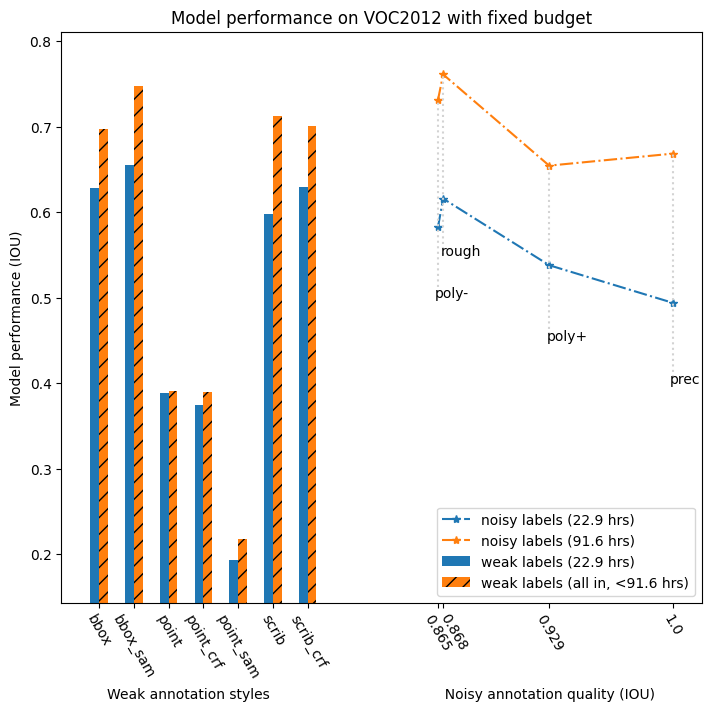
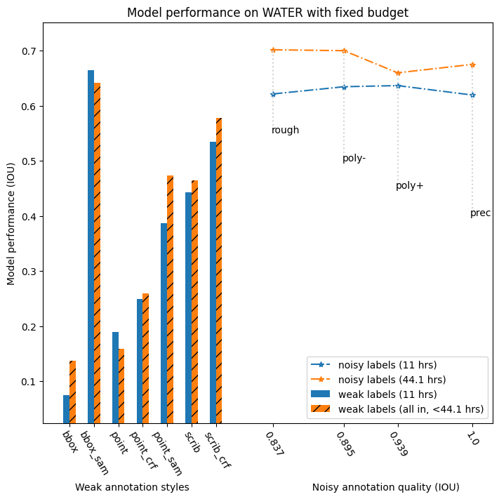
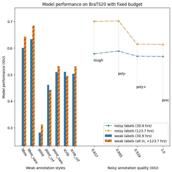
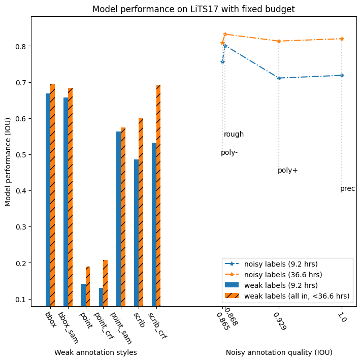
Figure 1: A comparison of annotation style efficacy with fixed annotation budgets

1 Introduction

Semantic segmentation is a well-researched topic in the field of computer vision. It has found a variety of practical applications. Segmentation neural networks typically employ Convolutional Neural Networks (CNNs) and/or Visual Transformers (ViTs) architectures. A notable challenge in training such models is the availability of segmentation labels, which typically comprise pixel-level segmentation masks. This is particularly the case where annotating data requires considerable professional expertise such as medical imaging.

Two main solutions emerged as remedies to alleviate the issue of limited precise segmentation labels. One is semi-supervised learning (SSL), which uses both annotated and unannotated data in the training process. Some common approaches include training feature extractors with 1) self-interpolation tasks [1, 2], 2) regularization with consistency to augmentation [3, 4], and 3) contrastive learning [5]. Fine-tuning will then occur on the task-relevant fully annotated images. The other solution is weakly-supervised semantic segmentation (WSSS), where imperfect labels are used to train the model. [6] WSSS trades annotation quality for more annotated images. Given annotations assumed in WSSS were not actual attempts to follow the boundaries of the objects of interest (in contrast to annotation with error/noise), they are also called “weak annotations”. Examples of weak annotations include points, scribbles, and bounding boxes. Here, we consider a practically important problem where one needs to annotate images but only has limited annotation budgets (time or money). Prior literature has not provided a systematic study of this issue with weak labels. We empirically analyze the cost-effectiveness of different annotation styles including both training supervision with weak and noisy annotations. Specifically, we include 1) fine polygons, 2) coarse polygons, 3) coarse contours, 4) bounding boxes, 5) scribbles, and 6) points, along with 7) precise annotations in our study. Our analysis provides a straightforward guide to those who are set on developing segmentation models and need to answer the question of how to invest their limited time into creating annotations. It also allows us to determine whether and to what extent one can use already existing weak annotations.

2 Related Work

Both noisy and weak labels have been previously used for annotation. Noisy annotations are made with annotators’ intent to quickly trace the outline of the object of interest. Though some boundary details may be lost, the areas of the objects are mostly preserved. In contrast, weak annotations are created to make an understandable reference to the object. Some prevalent examples of weak annotations are bounding boxes, points, and scribbles. We summarize literature relevant to the two types of annotations in this section.

2.1 Noisy Annotation

Unlike class label for image, which is either correct or incorrect, the more appropriate way to describe the errors in segmentation masks is the degree of imprecision. According to existing literature, imprecision in segmentation annotations showed some interesting characteristics: Heller et al. [7] demonstrated segmentation networks to experience uniform performance degradation as the errors in labels increase. Non-boundary-localized errors are less harmful than boundary-localized counterparts. Voronstov and Kadoury [8] showed segmentation networks to be resistant to varying degrees of random, unbiased errors. Zlateski et al. [9] conducted a study on the optimal quantity-quality trade-off of using coarse and polygon human annotation for trading models. Their results showed models trained on datasets containing a “higher number of imperfect labels” are more cost-effective than those containing a “lower number of precise labels” when the training budget is limited. Their study also mentioned the potential benefit of having a smaller precisely labeled training set for fine tuning. However, their study did not include weak annotations as potential candidates for annotation styles. In our study, we take both noisy annotations and weak annotations into consideration.

While only partially relevant to this study, we note that efforts also have been made to understand how errors in image labels affect model performance for the task of classification. Zhu et al. reported severe degradation in classification performance for statistical machine learning models when label noise was presented. [10] Xiao et al. proposed a label-noise-correction algorithm based on CNNs and probabilistic graphical models to predict and remove some suspected label errors in image datasets [11]. Jiang et al. proposed an ensemble learning algorithm to address label errors for classification when working with hyperspectral images [12]. A great variety of algorithms developed for working with erroneous classification labels can be found in different literature [13].

2.2 Weak Annotation

Directly training models with weak annotations such as points or scribbles rarely results in desirable performance. To employ them to train a mode, some label pre-processing or modifications of training frameworks are needed. Several algorithms have been developed for this purpose: for bounding box annotations, studies dated before 2018 such as Multiscale Combinatorial Grouping (MCG) [14], Simply Does It (SDI) [15], and GrabCut [16] leveraged object information with probabilistic graphical algorithms and feed the mask generated from weak annotations for model training. Subsequent work such as Box-drive Class-wise region Masking (BCM) [17], and Background Aware Pooling (BAP) [18] applied different priors and post-processing algorithms based on Conditional Random Field (CRF) for iterative mask updates rather than preparing the masks before the model training. For scribbles and point annotations, existing literature [19] tends to iteratively update the pseudo label based on some form of prediction uncertainty measures or training with specifically designed loss functions for sparse annotations [20]. Recent progress on models designed for interactive clicking segmentation (RITM [21], Focal Click [22]) or zero-short segmentation (Segment Anything [23]) has shown outstanding performance. It is made possible, though with limitations in some scenarios [24], to process weak annotations into high-quality dense masks for direct training supervision.

3 Data

We selected four segmentation datasets based on specific criteria. First, the ground truth annotations provided by each dataset need to be accurate, so that they are truly of superior quality than the weak/noisy annotations subsequently generated. Second, each dataset is expected to have a sufficiently large size of more than 2000 images so that labeling the whole dataset takes a non-trivial amount of time. This allows us to show the trend of model performance change as the annotation budget increases. Following these two criteria, we chose four datasets which covered both natural and medical images:

1. PASCAL VOC 2012 + BSDS500 labels (VOC) [25, 26]

2. ADE20K (water) + Water Segmentation Dataset + Satellite Images of Water Bodies [27, 28, 29]

3. Liver Tumor Segmentation Challenge (LiTS17) [30]

4. Multimodal Brain Tumor Segmentation Challenge 2020 (BraTS20) [31, 32, 33]

3.1 VOC2012

VOC2012 contains a total of 12031 images (2913 from VOC train and validation subset plus 9118 from BSDS500) for 20 classes of common objects. The images are split into the training set (varying size in our experiments, up to 10000 images), the validation set (582 images), and the test set (1449 images). This dataset is used for the task of multi-class segmentation.

3.2 WATER

WATER contains a total of 4070 images of water bodies, among which 1888 samples are from the water class in ADE20k, 404 samples are from water images filmed in the wild, and 1778 samples are from the ground truth annotations of satellite imagery. They were mixed and randomly split into a training set (up to 3648 images), a validation set (200 images), and a test set (200 images).

3.3 LiTS17

LiTS17 is preprocessed to have a total of 5501 2D slices extracted from 130 patients’ CT scans. We simplify this dataset to have only two classes: the foreground (liver + tumor on the liver) and the background (non-liver pixels). The dataset is split by the patient so that 4000 slices are used as the training set, 551 as the validation set, and 950 as the test set. The patients included in the training set are disjunct from those included in the test set.

3.4 BraTS20

BraTS20 is preprocessed to have a total of 16896 2D slices extracted from 369 patients’ MRI scans. Each slice contains a tumor region. This dataset contains volumes from T1, T1-CE, T2, and FLAIR sequences, together with a high-precision annotation for the GD-enhancing tumor, the peritumoral edema, and the necrotic and non-enhancing tumor cores, respectively with different labels. In our study, we use only the Flair sequence as network inputs and treat the different types of tumor tissues as one class. The dataset is split by the patient so that 10240 slices are used as the training set, 3692 as the validation set, and 2964 as the test set. The patients included in the training set are disjunct from those included in the test set.

4 Method

4.1 Annotation time estimation

To estimate the cost ratio between different annotation styles, we invited a human participant to label selected images using different annotation styles and recorded their annotation time. The participant was instructed to annotate 12 images with 7 annotation styles per image on the VOC and WATER datasets respectively. Since the participant is not trained to annotate MRI or CT images, we use the time estimation collected on VOC and WATER as a surrogation for LiTS17 and BraTS20. Table 1 summarizes the instruction given to the human participant.

Precise Annotation
Precise labels (prec)	original labels from the dataset
Noisy Annotations
Rought contour (rough)	rough continuous traces along the object contours
Fine polygon (poly+)	polygons with more vertexes on the object contours
Coarse polygon (poly-)	polygons with fewer vertexes on the object contours
Weak Annotations
Bounding box (bbox)	bounding boxes around each disconnected region of interest (ROI)
Scribble (scrib)	scribbles along the skeleton of each disconnected ROI
Point (point)	pixel mark near the center of the skeleton for each disconnected ROI

Table 1: Instructions made to annotators

The 12×7 image-annotation task pairs were presented to the participants in random order for a more accurate time estimation. The estimated ratio of time required is presented in Table. 2. and Fig.2

	prec	poly+	poly-	rough	bbox	scrib	point
VOC/LiTS17	1	1.18	3.13	3.35	5.00	5.56	7.02
WATER/BraTS20	1	1.33	3.58	5.43	9.76	1.084	10.09

Table 2: The average number of annotations one can make with the budget for one precise annotation

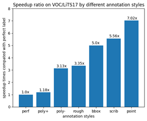
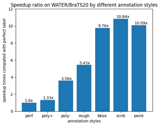
Figure 2: Annotation speedup for weak/noisy annotations

As a reference, we compare the ratio in our time estimation to the ratio of annotation price quotes from 7 annotation service providers. The quotes from 7 service providers follow a cost ratio of roughly 13:4:1 for precise (prec), coarse polygon (poly-), and bounding box (bbox) annotations. The cost ratio between prec and poly- matches very well with our time estimation. There was a slight difference between such cost estimate for prec vs. bbox in our estimate (9.76x and 5.0x for the two datasets) and the cost estimate (13x), however, a clear trend remained.

4.2 Simulating weak and noisy annotations

As stated in Sec. 2, our study considers both weak and noisy annotations. Noisy annotations include poly+, poly-, and rough as noisy annotations because they are effectively degraded versions of perf. On the other hand, bbox, scrib, and points are considered weak annotations since they are created to only give a reference to the object of interest. Since our study involves training models with the various types of weak/noisy annotations, a prerequisite step would be to generate convincing weak/noisy annotations from perf. In this section, we provide a detailed account of our protocols to generate weak and noisy annotations. We also listed the preprocessing and modification of training frameworks needed for noisy annotations. Fig.3 listed a visualization of all segmentation labels induced from the simulated weak/noisy annotations when iterative modification of the pseudo mask is not involved.

Dataset	Fine polygon (poly+)	Coarse polygon (poly-)	Coarse contour (rough)
VOC2012/LiTS17	0.929	0.865	0.868
WATER/BraTS20	0.939	0.895	0.837

Table 3: IoU of human-created noisy annotations versus precise annotations

Precise labels (prec): These are the original labels that come with the datasets, we consider them to be precise labels.

Fine polygon and coarse polygon (poly+, poly-): Polygon labels are created by approximating the boundaries of the precise labels with polygonal chains. The selected polygonal chains will end up enclosing a polygon region with non-trivial overlapping with the precise labels. In our study, we simulated these polygons using the cv2.approxPolyDP() function. By setting the “epsilon” parameter, we control the maximum distance between the polygonal line and the boundary to be estimated, thus also the quality of the polygon labels. Given our implementation, poly+ and poly- tend to have small Hausdorff distance with prec.

To determine the value for “epsilon” when generating labels, we compute the mean IOU (0.929) between the human-annotated poly+ and prec. Then, we manually selected a value for “epsilon” to generate poly+ labels with a mean IOU close to 0.929. For poly-, a similar procedure is used, except we aimed for a mean IOU of 0.865.

Coarse contour (rough): Rough labels simulate the products of an annotator quickly tracing along the objects’ boundaries. Unlike poly+ and poly- which preserves the Hausdorff distance with prec, rough focuses only on preserving the mass of the object. Details such as pointy edges may be erased. This is a different form of corruption to label quality, and we use the cv2.blur() function to mimic it. Similar to poly+ and poly-, we compute the mean IOU (0.868) between prec and human-annotated rough. Then, the filter size of cv2.blur() is manually adjusted so that the generated rough has the desired mean IOU to prec. Table 3 lists the mean IOU between the human-created noisy annotations and the precise labels. These numbers are used as a reference when controlling the parameters of cv2.approxPolyDP() and cv2.blur()

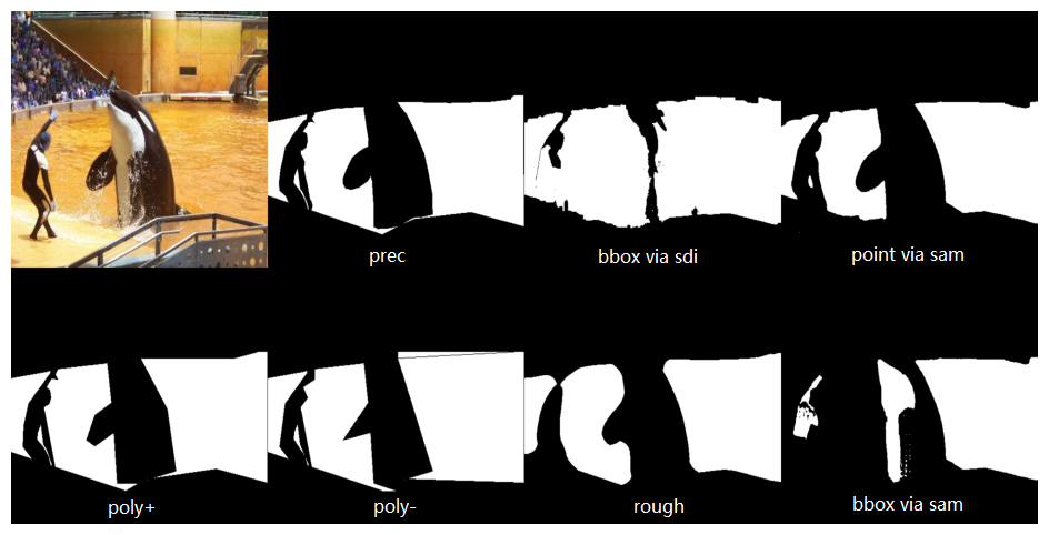
Figure 3: segmentation label induced from selected annotation styles

Bounding boxes (bbox, bbox_sam): Bounding boxes can be straightforwardly obtained by iterating through all indexes of the ROI pixels.

Scribbles (scrib, scrib_crf): The process of generating scribble annotations follows the auto-scribble generation protocols outlined in [34], whereby the scribbles are obtained through erosion of the pre-existing precise segmentation masks. A standard skeletonization procedure implemented as ‘skeletonize’ in Scikit-Image is performed iteratively and stops when the target object loses connectivity in the next iteration. Subsequently, the longest path along the skeleton is identified with fil_finder.FilFinder2D(). This pipeline gives us a visually realistic simulation of scribbles made by humans.

Points (point, point_crf, point_sam): Point annotation may be considered as a special case of scrib, where the scribble is 1 pixel long. In our implementation, we pick the pixel closest to the centroid of the scribble for each contiguous segment of interest. The background region is also assigned one and only one point, even if in some rare cases the background may contain multiple disconnected pieces. A potential drawback of this practice is that a crowd of N people may be assigned only one point rather than N points in total.

4.3 Model training with weak annotations

Weak annotations aimed at providing a conceptual reference to objects rather than providing an actual segmentation. They can barely be used directly for model training. Some pre-processing and modification of the training framework is needed. In this subsection, we elaborate on how weak annotations can be adapted for training supervision.

4.3.1 Bounding boxes (bbox, bbox_sam)

Graph-based approach: Khoreva et al. showed that preprocessing bounding box labels by naively filling the rectangles leads to models with poor performance. To address this issue, they proposed the SDI algorithm for generating pseudo-labels with better supervision capability. [15] Specifically, SDI merges the segmentation outputs from Multiscale Combinatorial Group (MCG) [14] and GrabCut [16] when given the bounding box. Pixels with disagreements between MCG and GrabCut are then marked as the ‘void’ class and excluded from gradient computing. Most subsequent literature adopted similar practices, so we believe the performance of SDI would be sufficiently representative. In our study, we denote the pseudo-labels obtained from SDI as bbox_sdi.

Foundation Models-based approach: Segment Anything (SAM) [23] was released in 2023 by Meta as a zero-shot instance segmentation model. It can produce a list of valid instance segmentation when given a bounding box prompt or a list of point prompts, without any assumptions on object semantics. Its emergence defines a new preprocessing paradigm of “preprocessing with large foundation models”. We denote the pseudo-labels output by SAM as bbox_sam.

4.3.2 Scribbles (scrib, scrib_crf)

Supervising model training with points may involve both label preprocessing and modifications to the training framework. We adopted two versions of algorithms with scribble annotations.

Version 1 (denoted as scrib) started with applying GrabCut on the scribble and used the output as the pseudo mask for training supervision. In each training iteration, a pseudo label is generated following the formula $Y_{t}=GrabCut(X,S_{t-1})$, where $S_{t-1}$ is the model output from the previous iteration. Then, the training is supervised by the CrossEntropyLoss between $S_{t}$ and $Y_{t}$. The model and GrabCut interweavingly update each other until the loss converges.

Version 2 (denoted as scrib_crf) dropped the explicit inference step of GrabCut by attaching a DenseCRF [35] head to the model. The loss on the DenseCRF head is the CRFLoss, which serves as a regularization term on the model output. Conceptually, this modification simulates GrabCut with a sub-module of the network and optimizes the two components in an end-to-end manner. The final loss function in version 2 takes the form:

$$L_{t}=\sum_{i\in N}CrossEntropy(Y_{t}^{(i)},S_{t}^{(i)})+\lambda CRFLoss(S_{t}^{(i)})$$

In our experiments, $\lambda$ is set to be 1e-9.

4.3.3 Scribbles (scrib, scrib_crf)

Supervising model training with points may involve both label preprocessing and modifications to the training framework. We adopted two versions of algorithms with scribble annotations. Version 1 (denoted as scrib) started with applying GrabCut on the scribble and used the output as the pseudo mask for training supervision. In each training iteration, a pseudo label is generated following the formula $Y_{t}=GrabCut(X,S_{t-1})$, where $S_{t-1}$ is the model output from the previous iteration. Then, the training is supervised by the CrossEntropyLoss between $S_{t}$ and $Y_{t}$. The model and GrabCut interweavingly update each other until the loss converges. Version 2 (denoted as scrib_crf ) dropped the explicit inference step of GrabCut by attaching a DenseCRF [35] head to the model. The loss on the DenseCRF head is the CRFLoss, which serves as a regularization term on the model output. Conceptually, this modification simulates GrabCut with a sub-module of the network and optimizes the two components in an end-to-end manner. The final loss function in version 2 takes the form:

$$L_{t}=\sum_{i\in N}CrossEntropy(Y_{t}^{(i)},S_{t}^{(i)})+\lambda CRFLoss(S_{t}^{(i)})$$

In our experiments, $\lambda$ is set to be 1e-9.

4.3.4 Points (point, point_crf, point_sam)

During model training with points, we adopt three versions of training frameworks. Two versions have been introduced in the previous subsection for scribbles, denoted as point and point_crf. They are effectively special cases for scrib and scrib_crf. The third version was to preprocess point prompts with SAM, which outputs segmentation masks and requires no modification on the training framework (denoted as point_sam). The segmentation masks with the highest confidence score by SAM are used as the label for model training.

5 Experimental design and model training

To compare and find the most cost-effective annotation type for segmentation tasks, we control the available annotation time budget and evaluate model performance for different budgets. Specifically, the budget levels increase by a factor of two until all available images in the training set can be precisely annotated. If there are not enough images to consume all the budget, we simply train the model using all the labeled data available. By the end of all experiments, we expect to collect a 2D plot with the annotation budget on the x-axis and the related model performance (mIOU or IOU of the target class) on the y-axis.

For each dataset, we use different CNN architectures and/or optimization hyperparameters with minimal hyperparameter tunning. We report the detailed training setup and the associated model performance in this section for all four datasets. We plot the experiment result for each (time constraint, annotation style) pair for VOC2012, WATRE, LiTS17, and BraTS20 in Fig.4 and Fig.5, whose x-axis represents time constraint, the y-axis represents model performance, and the line color represents annotation style. For the same annotation time (x-value), higher mIOU (y-value) implies higher annotation cost-effectiveness.

5.1 VOC2012

For VOC2012, we follow the official implementation of the PSP-Net with Resnet 101 backbone and their training protocol, both of which are available on GitHub. However, we reduced the input patch size from 473 to 393 due to the memory constraints of our GPUs. For each (time constraint, annotation style) pair P, we validate the model performance after each training epoch and save the models’ weights achieving the highest 3 validation mIoUs.

5.2 WATER

For WATER, we use DeepLabV3 with Resnet-50 backbone pre-trained with ImageNet. The model is trained using Adam optimizer with lr = 1e-3 on cross-entropy loss. For the training and validation set, images are augmented with ColorJitter and RandomEqualize with p = 0.5. Then, they are padded to square and resized to $256\times 256$. For each (time constraint, annotation style) pair, we validate the model after each training epoch. The one with the highest mean validation IOUs for the background and foreground is saved as the final model for the (time constraint, annotation style) pair. We use this dataset for binary segmentation tasks and report the segmentation IOU of the water class.

5.3 LiTS17

For LiTS17, we crop patches from each image without resizing and train a vanilla UNet with default initialization for the liver class. The optimizer used is SGD with lr = 0.01, momentum = 0.9, weight_decay = 1e-5. A weight scheduling policy is used by multiplying the learning rate by 0.1 every 3000 iterations. In addition, we dynamically adjust the weight of each class based on their validation IOU. The validation IOU for each class from the previous training epoch is used to compute the relative weight for the cross-entropy loss. The specific formula used is For each (time constraint, annotation style) pair, we cache the model trained at the epoch that obtains the highest mean validation IOU as the final model along its training. We use this dataset for binary segmentation tasks and report the segmentation IOU of the liver class.

5.4 BraTS20

For BraTS20, we use only the Flair sequence of the MRI volumes and treat all tumor subclasses as a single “tumor” class. Each slice comes natively with a size of $240\times 240$. The InceptionUNet is adapted as our segmentation network. The optimizer configuration, class weight adjustment policy, and model selection mechanism are held the same as used for the WATER dataset. We use this dataset for binary tumor segmentation tasks and report the segmentation IOU on the union of all tumor-affected regions read through all MRI sequences (i.e., T1, T1CE, T2, and Flair).

6 Results

6.1 VOC2012

The experiments on VOC2012 (Fig.4(a))show that most styles of weak/noisy annotations have higher cost-effectiveness than precise annotations. Among them, SAM-generated masks with bounding box prompts (bbox_sam) achieved the highest cost-effectiveness, followed by coarse contour labels (rough). This is not very surprising given the performance of SAM.

Despite the high cost-effectiveness of SAM with bounding box prompt, SAM with point prompt is underperforming. We found that the highest-confidence label with point prompts produced by SAM tends to only include a small sub-component of the target region. For example, if a point is assigned to the window of a car, then only that specific piece of window will be marked as the target. Due to the ambiguity of what a single point could refer to, SAM did not stably generate satisfactory pseudo masks without subsequent human feedback. Also, SAM is designed for instance segmentation. It picks only one instance from a crowd of objects when given only one point label. These factors all contribute to the low performance of point_sam. Point annotations with iterative training, unfortunately, though showed higher cost-effectiveness than point_sam, still rank the lowest among the rest of the candidate’s annotation styles.

Fine polygon annotations showed similar cost-effectiveness as precise annotations. This is expected because generating high-precision polygon annotations takes a similar time to generating precise annotations. Plus, as expected, none of the models trained with weak annotations outperform the model trained with all the precise labels when all available training images are included.

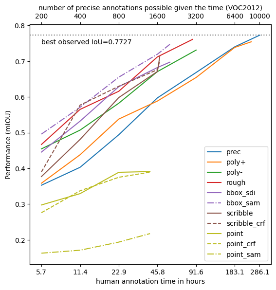
(a) Model performance with different annotation styles at increasing budget on VOC2012

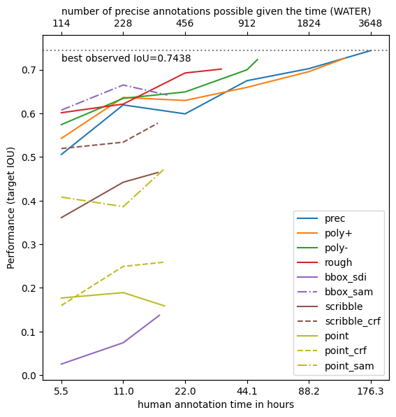
(b) Model performance with different annotation styles at increasing budget on WATER

Figure 4: Cost effectiveness of different annotation styles on natural images

6.2 WATER

Like VOC2012, coarse polygon (poly-) and coarse contour (rough) annotations consistently show better cost-effectiveness than precise annotations. Fine polygon annotations have similar performance to precise annotations. For scribble labels, both the variants with and without integrating CRF loss during training, their performance is not comparable to polygon annotations and contour labels. The bounding box masks generated with SDI failed to train a model with a reasonable prediction capability in this experiment. One potential cause for this observation could be the dataset itself. Unlike in VOC where ROIs are typically complete (without holes) and can be a hierarchical combination of multiple subcomponents, ROIs in WATER represent the concept of “stuff” rather than “object”. Also, due to the erratic shapes of some water bodies, sometimes a bounding box may cover multiple objects and introduce great ambiguity in the annotation. Interestingly, unlike SDI, SAM had a decent, though fast saturating performance with bounding box prompts. The two versions of point annotations with iterative training have low cost-effectiveness and saturating performance. (See Fig.4(b))

6.3 LiTS17

For LiTS17, coarse polygon (poly-) and coarse contour (rough) labels remain to have higher cost-effectiveness than the precise labels. The performance of models trained with the two variants of bounding box labels and scribble labels saturated quickly with an IOU marginally higher than 0.65. Plus, bounding box labels always yield higher cost-effectiveness than scribble labels in this dataset. Coarse contour labels result in models with higher performance than both high-precision and coarse polygon annotations as available annotation time increases. This higher performance may be caused by the nature of coarse contours, which have smooth boundaries that more closely resemble the boundaries of livers than the vertex-based annotations. All variants of scribble annotations and point annotations yield lower cost-effectiveness than precise annotations. Again, point annotations with iterative training have the lowest performance when all training images are used. (See Fig.5(a))

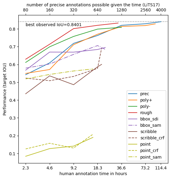
(a) Model performance with different annotation styles at increasing budget on LiTS17

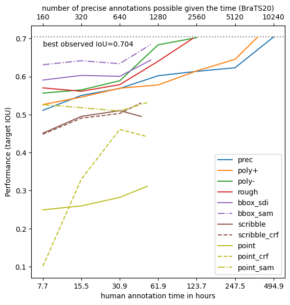
(b) Model performance with different annotation styles at increasing budget on BraTS20

Figure 5: Cost effectiveness of different annotation styles on CT and MRI images

6.4 BraTS20

For BraTS20, we found models trained with the three types of noisy annotations achieve similar maximum performance to that of precise annotations. We attribute this observation to the inherent challenges in recognizing tumor regions with only information in the FLAIR sequence: the contrast between tumor and non-tumor regions may be low, making some tumor boundaries obscure on the FLAIR sequence. Both variants of bounding box annotations achieve high cost-effectiveness. The bounding box annotation preprocessed with SAM again achieves the highest cost-effectiveness and moderately high performance when all training images are included. All variants of point annotation and scribble annotations have less favorable cost-effectiveness and performance than precise annotations. (See Fig.5(b))

Through experiments on these four datasets, we observe some common phenomena:

1. Noisy annotations with a moderate level of error (poly-, rough) are more cost-effective than precise annotations.

2. Training models with noisy annotations would not result in a significant compromise in model performance for the same set of training images.

3. When labeling object-like ROIs, creating bounding box annotation and post-processing with zero-shot segmentation networks (e.g., SAM, RITM, SimpleClick…) could be a highly cost-effective data-labeling pipeline.

6.5 Effects of noise level on model performance

In the previous experiments, most models trained on weak/noisy annotations obtained higher performance than the perf counterpart when given the same annotation budget. This observation holds until all unlabeled images are exhausted. Annotation quality seemed to play a lesser role. However, for the comprehensiveness of our study, we analyze its impact in an isolated manner. Specifically, we change the parameters for generating coarse contour labels (rough) such that the mIoUs between rough and prec are equal to [0.81, 0.84, 0.87, 0.90, 0.93]. A model is trained on each of the five variants of rough labels with incremental quality. The impact of the annotation quality of rough is then quantitatively analyzed with Spearman correlation against the performance of the five models. (See Fig.6)

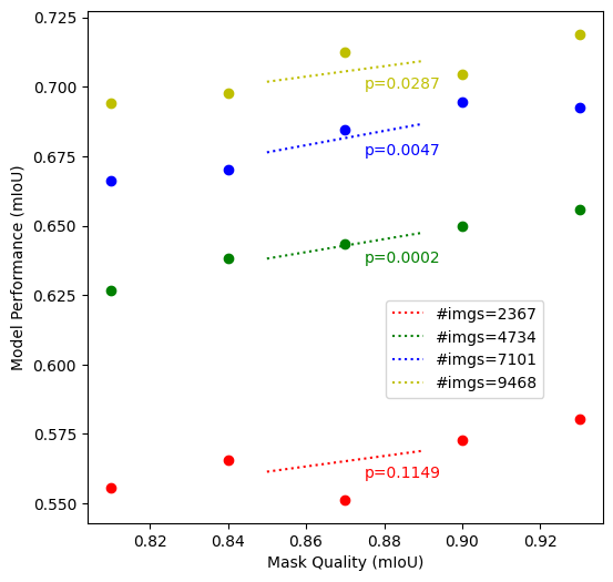
(a) Effects of mask quality (VOC2012)

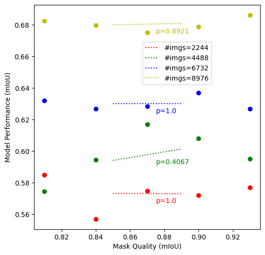
(b) Effects of mask quality (BraTS20)

Figure 6: Effects of training mask quality on model performance with fixed sample counts

In VOC2012, a statistically significant (p$<$0.05) trend of increase in model performance is observed for rough labels with higher quality. However, reducing the mask error rate by half caused only a marginal improvement in model performance than double the training size. In BraTS20, no statistically significant trend is observed for changing the quality of the mask in the IoU range (0.81 0.93) for any training set size. The possible cause is as explained in Section 6.4, that there exists an inherence uncertainty even for humans to determine the boundary of tumors from merely the FLAIR sequence. Still, following the results shown in Fig.6(a), refining mask quality may contribute to a further improvement in model performance when all available images are already included for training.

7 Discussion and Conclusion

In our study, we explored the cost-effectiveness of different weak and noisy annotation styles and their capability of supervising the training of a segmentation network. We found that in all four datasets, using coarse polygon (poly-), coarse contour (rough) and sometimes bounding box annotations with SAM pre-processing (bbox_sam) to train the segmentation model results in models with higher cost-effectiveness than training with precise annotations. Using the weak/noisy annotation styles may lead to a 66% $\sim$ 90% reduction in annotation cost with minimal compromise in model performance (0.01$\sim$0.05 decrease in mIoU). Also, we verified that within a reasonable parameter space (mIoU$>$0.8), the impact of annotation quality is minor and may be overridden by the impact of having more examples, which could be a complement to the conclusion in Sec. 6.4.

We also found single-point annotations (without considering point_sam) to be of inferior performance and cost-effectiveness to both variants of scribbles (scrib). This is unsurprising since it takes a similar amount of time to make the point and scribble labels, yet scribbles may cross multiple regions with different textures. In our study, we did not analyze the effects of integrating scribbles with foundation models, yet doing so has the potential to bring a competitive candidate annotation style. Future work may also consider a 3D version of our study in the field of medical imaging. In medical images, MRI and CT images come in the form of volumes, with each volume containing hundreds of slices. Researchers in medical image segmentation may benefit from a study similar to ours but with 3D tasks.

Our study has some limitations. First, for simplicity, we assumed each training set to contain a homogeneous annotation style. However, in practice, mixed styles of annotations may be present in a dataset. One may even further apply semi-supervised learning in conjunction with the weak annotations to leverage the unlabeled data. Second, for scribble/point annotations, there is further room for investigation on how the tune the prompt for the interactive segmentation models. (e.g., N points per object, where to drop the point). However, our study assumed each object has only one scribble/point annotation. Lastly, the performance of BraTS20 and VOC2012 hasn’t fully reached the saturation point for some annotation styles. Despite so, our experiments still cover four moderately large datasets to make the results representative of what could be expected in a real-life scenario.

In conclusion, we recommend weak/noisy annotations with reasonable quality (mIOU$>$0.83) to be adopted when the unlabeled images are abundant and the annotation budget is a limiting factor. In contrast, if time is not a constraint but rather the number of unlabeled samples, improving annotation quality can still definitely, though slightly, improve model performance. We do not recommend annotating data with single-point annotation in all circumstances.

References

- He et al. [2022] K. He, X. Chen, S. Xie, Y. Li, P. Dollár, R. Girshick, Masked autoencoders are scalable vision learners, in: 2022 IEEE/CVF Conference on Computer Vision and Pattern Recognition (CVPR), 2022, pp. 15979–15988. doi:10.1109/CVPR52688.2022.01553.
- Xie et al. [2022] Z. Xie, Z. Zhang, Y. Cao, Y. Lin, J. Bao, Z. Yao, Q. Dai, H. Hu, Simmim: a simple framework for masked image modeling, in: 2022 IEEE/CVF Conference on Computer Vision and Pattern Recognition (CVPR), 2022, pp. 9643–9653. doi:10.1109/CVPR52688.2022.00943.
- Chen et al. [2021] X. Chen, Y. Yuan, G. Zeng, J. Wang, Semi-supervised semantic segmentation with cross pseudo supervision, in: Proceedings of the IEEE/CVF Conference on Computer Vision and Pattern Recognition, 2021, pp. 2613–2622.
- Ouali et al. [2020] Y. Ouali, C. Hudelot, M. Tami, Semi-supervised semantic segmentation with cross-consistency training, in: Proceedings of the IEEE/CVF Conference on Computer Vision and Pattern Recognition, 2020, pp. 12674–12684.
- Chen et al. [2020] T. Chen, S. Kornblith, M. Norouzi, G. Hinton, A simple framework for contrastive learning of visual representations, in: International conference on machine learning, PMLR, 2020, pp. 1597–1607.
- Papandreou et al. [2015] G. Papandreou, L.-C. Chen, K. P. Murphy, A. L. Yuille, Weakly-and semi-supervised learning of a deep convolutional network for semantic image segmentation, in: Proceedings of the IEEE international conference on computer vision, 2015, pp. 1742–1750.
- Heller et al. [2018] N. Heller, J. Dean, N. Papanikolopoulos, Imperfect segmentation labels: How much do they matter?, in: Intravascular Imaging and Computer Assisted Stenting and Large-Scale Annotation of Biomedical Data and Expert Label Synthesis: 7th Joint International Workshop, CVII-STENT 2018 and Third International Workshop, LABELS 2018, Held in Conjunction with MICCAI 2018, Granada, Spain, September 16, 2018, Proceedings 3, Springer, 2018, pp. 112–120.
- Vorontsov and Kadoury [2021] E. Vorontsov, S. Kadoury, Label noise in segmentation networks: mitigation must deal with bias, in: Deep Generative Models, and Data Augmentation, Labelling, and Imperfections: First Workshop, DGM4MICCAI 2021, and First Workshop, DALI 2021, Held in Conjunction with MICCAI 2021, Strasbourg, France, October 1, 2021, Proceedings 1, Springer, 2021, pp. 251–258.
- Zlateski et al. [2018] A. Zlateski, R. Jaroensri, P. Sharma, F. Durand, On the importance of label quality for semantic segmentation, in: Proceedings of the IEEE Conference on Computer Vision and Pattern Recognition, 2018, pp. 1479–1487.
- Zhu and Wu [2004] X. Zhu, X. Wu, Class noise vs. attribute noise: A quantitative study, Artificial intelligence review 22 (2004) 177–210.
- Xiao et al. [2015] T. Xiao, T. Xia, Y. Yang, C. Huang, X. Wang, Learning from massive noisy labeled data for image classification, in: Proceedings of the IEEE conference on computer vision and pattern recognition, 2015, pp. 2691–2699.
- Jiang et al. [2018] J. Jiang, J. Ma, Z. Wang, C. Chen, X. Liu, Hyperspectral image classification in the presence of noisy labels, IEEE Transactions on Geoscience and Remote Sensing 57 (2018) 851–865.
- Algan and Ulusoy [2021] G. Algan, I. Ulusoy, Image classification with deep learning in the presence of noisy labels: A survey, Knowledge-Based Systems 215 (2021) 106771.
- Arbeláez et al. [2014] P. Arbeláez, J. Pont-Tuset, J. T. Barron, F. Marques, J. Malik, Multiscale combinatorial grouping, in: Proceedings of the IEEE conference on computer vision and pattern recognition, 2014, pp. 328–335.
- Khoreva et al. [2017] A. Khoreva, R. Benenson, J. Hosang, M. Hein, B. Schiele, Simple does it: Weakly supervised instance and semantic segmentation, in: Proceedings of the IEEE conference on computer vision and pattern recognition, 2017, pp. 876–885.
- Rother et al. [2004] C. Rother, V. Kolmogorov, A. Blake, ” grabcut” interactive foreground extraction using iterated graph cuts, ACM transactions on graphics (TOG) 23 (2004) 309–314.
- Song et al. [2019] C. Song, Y. Huang, W. Ouyang, L. Wang, Box-driven class-wise region masking and filling rate guided loss for weakly supervised semantic segmentation, in: Proceedings of the IEEE/CVF Conference on Computer Vision and Pattern Recognition, 2019, pp. 3136–3145.
- Oh et al. [2021] Y. Oh, B. Kim, B. Ham, Background-aware pooling and noise-aware loss for weakly-supervised semantic segmentation, in: Proceedings of the IEEE/CVF Conference on Computer Vision and Pattern Recognition, 2021, pp. 6913–6922.
- Can et al. [2018] Y. B. Can, K. Chaitanya, B. Mustafa, L. M. Koch, E. Konukoglu, C. F. Baumgartner, Learning to segment medical images with scribble-supervision alone, in: Deep Learning in Medical Image Analysis and Multimodal Learning for Clinical Decision Support: 4th International Workshop, DLMIA 2018, and 8th International Workshop, ML-CDS 2018, Held in Conjunction with MICCAI 2018, Granada, Spain, September 20, 2018, Proceedings 4, Springer, 2018, pp. 236–244.
- Tang et al. [2018] M. Tang, F. Perazzi, A. Djelouah, I. Ben Ayed, C. Schroers, Y. Boykov, On regularized losses for weakly-supervised cnn segmentation, in: Proceedings of the European Conference on Computer Vision (ECCV), 2018, pp. 507–522.
- Sofiiuk et al. [2022] K. Sofiiuk, I. A. Petrov, A. Konushin, Reviving iterative training with mask guidance for interactive segmentation, in: 2022 IEEE International Conference on Image Processing (ICIP), IEEE, 2022, pp. 3141–3145.
- Chen et al. [2022] X. Chen, Z. Zhao, Y. Zhang, M. Duan, D. Qi, H. Zhao, Focalclick: Towards practical interactive image segmentation, in: Proceedings of the IEEE/CVF Conference on Computer Vision and Pattern Recognition, 2022, pp. 1300–1309.
- Kirillov et al. [2023] A. Kirillov, E. Mintun, N. Ravi, H. Mao, C. Rolland, L. Gustafson, T. Xiao, S. Whitehead, A. C. Berg, W.-Y. Lo, et al., Segment anything, arXiv preprint arXiv:2304.02643 (2023).
- Mazurowski et al. [2023] M. A. Mazurowski, H. Dong, H. Gu, J. Yang, N. Konz, Y. Zhang, Segment anything model for medical image analysis: an experimental study, Medical Image Analysis 89 (2023) 102918.
- Everingham et al. [????] M. Everingham, L. Van Gool, C. K. I. Williams, J. Winn, A. Zisserman, The PASCAL Visual Object Classes Challenge 2012 (VOC2012) Results, http://www.pascal-network.org/challenges/VOC/voc2012/workshop/index.html, ????
- Martin et al. [2001] D. Martin, C. Fowlkes, D. Tal, J. Malik, A database of human segmented natural images and its application to evaluating segmentation algorithms and measuring ecological statistics, in: Proc. 8th Int’l Conf. Computer Vision, volume 2, 2001, pp. 416–423.
- Liang et al. [2020] Y. Liang, N. Jafari, X. Luo, Q. Chen, Y. Cao, X. Li, Waternet: An adaptive matching pipeline for segmenting water with volatile appearance, Computational Visual Media (2020) 1–14.
- Zhou et al. [2017] B. Zhou, H. Zhao, X. Puig, S. Fidler, A. Barriuso, A. Torralba, Scene parsing through ade20k dataset, in: Proceedings of the IEEE Conference on Computer Vision and Pattern Recognition, 2017.
- Zhou et al. [2019] B. Zhou, H. Zhao, X. Puig, T. Xiao, S. Fidler, A. Barriuso, A. Torralba, Semantic understanding of scenes through the ade20k dataset, International Journal of Computer Vision 127 (2019) 302–321.
- Bilic et al. [2023] P. Bilic, P. Christ, H. B. Li, E. Vorontsov, A. Ben-Cohen, G. Kaissis, A. Szeskin, C. Jacobs, G. E. H. Mamani, G. Chartrand, et al., The liver tumor segmentation benchmark (lits), Medical Image Analysis 84 (2023) 102680.
- Menze et al. [2014] B. H. Menze, A. Jakab, S. Bauer, J. Kalpathy-Cramer, K. Farahani, J. Kirby, Y. Burren, N. Porz, J. Slotboom, R. Wiest, et al., The multimodal brain tumor image segmentation benchmark (brats), IEEE transactions on medical imaging 34 (2014) 1993–2024.
- Bakas et al. [2017] S. Bakas, H. Akbari, A. Sotiras, M. Bilello, M. Rozycki, J. S. Kirby, J. B. Freymann, K. Farahani, C. Davatzikos, Advancing the cancer genome atlas glioma mri collections with expert segmentation labels and radiomic features, Scientific data 4 (2017) 1–13.
- Bakas et al. [2018] S. Bakas, M. Reyes, A. Jakab, S. Bauer, M. Rempfler, A. Crimi, R. T. Shinohara, C. Berger, S. M. Ha, M. Rozycki, et al., Identifying the best machine learning algorithms for brain tumor segmentation, progression assessment, and overall survival prediction in the brats challenge, arXiv preprint arXiv:1811.02629 (2018).
- Valvano et al. [2021] G. Valvano, A. Leo, S. A. Tsaftaris, Learning to segment from scribbles using multi-scale adversarial attention gates, IEEE Transactions on Medical Imaging 40 (2021) 1990–2001.
- Chen et al. [2015] L. Chen, G. Papandreou, I. Kokkinos, K. Murphy, A. L. Yuille, Semantic image segmentation with deep convolutional nets and fully connected crfs, in: Y. Bengio, Y. LeCun (Eds.), 3rd International Conference on Learning Representations, ICLR 2015, San Diego, CA, USA, May 7-9, 2015, Conference Track Proceedings, 2015. URL: http://arxiv.org/abs/1412.7062.