Mediation Analysis with Mendelian Randomization
and Efficient Multiple GWAS Integration

Abstract

Mediation analysis is a powerful tool for studying causal pathways between exposure, mediator, and outcome variables of interest. While classical mediation analysis using observational data often requires strong and sometimes unrealistic assumptions, such as unconfoundedness, Mendelian Randomization (MR) avoids unmeasured confounding bias by employing genetic variants as instrumental variables. We develop a novel MR framework for mediation analysis with genome-wide associate study (GWAS) summary data, and provide solid statistical guarantees. Our framework efficiently integrates information stored in three independent GWAS summary data and mitigates the commonly encountered winner’s curse and measurement error bias (a.k.a. instrument selection and weak instrument bias) in MR. As a result, our framework provides valid statistical inference for both direct and mediation effects with enhanced statistical efficiency. As part of this endeavor, we also demonstrate that the concept of winner’s curse bias in mediation analysis with MR and summary data is more complex than previously documented in the classical two-sample MR literature, requiring special treatments to address such a bias issue. Through our theoretical investigations, we show that the proposed method delivers consistent and asymptotically normally distributed causal effect estimates. We illustrate the finite-sample performance of our approach through simulation experiments and a case study.

Keywords: Inverse Variance Weighting; Post-selection Inference; Increasing Dimension; Instrumental Variable; Mediation Analysis.

1 Introduction

1.1 Background and contribution

Mediation analysis is a powerful tool for studying causal pathways between exposure, mediator, and outcome variables of interest. It offers a systematic framework to disentangle the direct effect of the exposure on the outcome and the indirect effect that runs through the mediator. Nevertheless, classical mediation analysis using observational data often requires strong and sometimes unrealistic assumptions, such as no unmeasured confounders in the mediator-outcome relationship. When such assumptions are violated, classical mediation analysis may produce biased causal effect estimates. While Mendelian Randomization (MR) offers a strategy to mitigate such unmeasured confounding bias by employing genetic variants as instrumental variables (IVs) (Carter et al., 2021), it has been traditionally adopted to estimate the total causal effect between the exposure and outcome variables, implying a need for careful customization of MR for mediation analysis.

In this manuscript, we develop a unified Mendelian randomization framework for mediation analysis with genome-wide associate study (GWAS) summary data. We choose the research design with GWAS summary data because of the public availability of such data and the extensive breadth of traits covered by GWAS with substantial sample sizes. For example, the GWAS Catalog contains summary statistics from more than $45,000$ individual GWAS across over $6,000$ publications (Sollis et al., 2023). Such resources allow researchers to analyze a broad range of exposures, mediators, and outcomes with high statistical precision, even for relatively rare outcomes. To the best of our knowledge, this is the first MR framework incorporating GWAS summary data which (i) is specifically tailored for mediation analysis, (ii) effectively addresses both the winner’s and loser’s curse as well as measurement error bias (detailed discussions on relevant bias sources can be found in Section 2), (iii) remains valid even when instrument selection is imperfect, and (iv) enjoys solid theoretical guarantees. In what follows, we discuss our contributions in more detail.

On the statistical methodology side, our framework efficiently integrates information stored in three independent GWAS summary data and mitigates the commonly encountered winner’s curse and measurement error bias in MR. As a part of this endeavor, we show that the winner’s curse concept in mediation analysis with MR and summary data is considerably more complex than previously documented in the classical two-sample MR literature, as IV selection in mediation analysis induces both winner’s and loser’s curses (Section 2). Moreover, we also demonstrate the impact of imperfect IV selection for mediation analysis using MR with summary data. While imperfect IV selection may not have a substantial impact on parameter estimation in two-sample MR, it can result in either efficiency loss or/and estimation bias in mediation analysis using MR (Section 2). Our proposed approach is free of the aforementioned potential sources of bias.

As our framework successfully addresses the above-mentioned bias issues, it provides valid statistical inference for both direct and mediation effects with enhanced statistical efficiency. Here, the efficiency gain stems from carefully constructing three estimating equations Eq (3)–(5). These unique estimating equations allow us to form efficient direct effects and mediation effect estimators using solely the IVs that are either relevant to the exposure variable or the mediator. This approach differs from multivariable MR analysis, which uses the union of all relevant IVs of the exposure and the mediator.

From a theoretical perspective, we first establish a joint asymptotic normality result for the causal effect estimators of both direct and indirect effects, allowing both the sample size and the number of IVs to diverge, as indicated in Theorem 1. As these estimators are correctly centered at their population targets, this result demonstrates our estimators are free of both winner’s curse bias and measurement error bias concerns. We next provide a consistent estimator of the covariance matrix in Theorem 1, enabling us to construct valid confidence intervals for desired causal effects, as well as their combinations based on the delta method. Furthermore, we demonstrate in a simplified scenario that our proposed estimators indeed offer asymptotic efficiency gain over those derived from multivariable MR analysis, as shown in Theorem 2.

On the practical side, we showcase the finite-sample performance of our framework through Monte Carlo experiments (Section 5) and a case study (Section 6). Through these results, we demonstrate that our approach (i) provides accurate estimates for both direct and mediation effects, (ii) exhibits superior performance in terms of boosted power, improved coverage, and reduced bias compared to several existing methods, and (iii) has lower variance than the (debiased) multivariable MR estimator. In the case study, our proposed approach identifies more significant pathways than the mediation analysis conducted using classical MR.

1.2 Existing literature

Two MR methods using summary data are available in the literature for mediation analysis: two-step MR and multivariable MR (MVMR). However, it is unclear if these two approaches provide valid statistical inference on the direct and mediation effects. In what follows, we give a review of both methods, followed by their potential limitations; also see Table 2 for a summary.

Two-step MR employs univariate MR analysis in a two-step fashion to estimate the mediation effect (Evans and Davey Smith, 2015; Burgess et al., 2014; Relton and Davey Smith, 2012). More concretely, it first estimates the causal effect of the exposure to the mediator using the IVs that are relevant to the exposure variable, and then, similarly, estimates the causal effect of the mediator to the outcome using the IVs that are relevant to the mediator (Carter et al., 2021). The product of the estimated effects steps gives the final mediation effect estimation. The standard errors of the mediation effect is subsequently obtained through the delta method. Note that an extra third step, a univariate MR regression of the exposure on the outcome, is needed if one is interested in decomposing the total effect of the exposure.

MVMR extends the framework of univariate MR, enabling the estimation of direct effects from multiple exposures on an outcome variable (Burgess and Thompson, 2015; Grant and Burgess, 2021; Sanderson, 2021). To use MVMR for estimating mediation effects, it is possible to first obtain the total effect of the exposure on the outcome variable via univariate MR, and then subtract the direct effect obtained via MVMR from the estimated total effect, yielding the estimate of the mediation effect.

The above mediation analysis methods built upon two-step MR and MVMR suffer from the well-recognized measurement error and winner’s curse bias issues (Gkatzionis and Burgess, 2019; Sadreev et al., 2021; Smith, 1981; Robertson et al., 2016). On the one hand, the measurement error bias arises because GWAS summary statistics (i.e., associations with the instruments) are estimated with errors. Existing literature on univariate MR also refers to this measurement error bias as the weak IV bias; see Sadreev et al. (2021); Bowden et al. (2016, 2019); Jiang and Ding (2020); Zhao et al. (2020); Ye et al. (2021), and Ma et al. (2023) for more discussions on how measurement error bias leads to attenuated causal effects. Unlike univariate MR, measurement error bias in MVMR and two-step MR is jointly determined by the directions and magnitudes of direct effects, making its impact on causal effect estimates complex and unclear. On the other hand, the winner’s curse arises in MR analysis whenever the same GWAS sample is used to select relevant IVs and to estimate their associations (with the exposure or the mediator). While the impact of winner’s bias is well understood in univariate MR (Sadreev et al., 2021), its manifestation in mediation analysis using multiple GWAS is less clear.

Figure 1: Causal diagram for mediation analysis with multiple GWAS.

Furthermore, solid theoretical guarantee for two-step MR and MVMR is lacking in the literature. For example, two-step MR relies on the delta method to construct standard error for the estimated mediation effect, and common practice precludes shared instruments from being used for both the exposure and the mediator. Whenever this condition fails, causal effect estimates (more precisely, estimates of $\tau_{X}$ and $\tau_{Y}$ in Figure 1) from two-step MR can be correlated, and constructing standard errors based on two-step MR becomes problematic and challenging. A similar issue arises in MVMR, as no method is available for statistical inference on mediation effects.

In this manuscript, we establish a unified framework for mediation analysis with multiple GWAS, in which we provide accurate direct and mediation effect estimates with valid statistical inference.

2 Mediation analysis with MR and summary data: challenges

In Table 1 below, we introduce the mediation analysis framework with three independent GWAS based on the causal diagram of Figure 1. We note that our framework avoids the winner’s curse bias and thus does not require additional independent GWAS for SNP selection. The GWAS summary statistics are obtained by regressing the exposure, outcome, and mediator separately on each SNP in the corresponding exposure/outcome/mediator datasets and then recording marginal regression coefficients and standard errors.

	Individual-level dataaaa	Publicly available summary data
GWAS (I): Exposure dataset	$\Big{\{}\big{(}X_{i}^{*},G_{ij}^{*}\big{)}\Big{\}}_{i=1}^{n_{X}}$	$\Big{\{}\big{(}\widehat{\beta}_{X_{j}},\sigma_{X_{j}}^{2}\big{)}\Big{\}}_{j=1}^{p}$
GWAS (II): Outcome dataset	$\Big{\{}\big{(}Y_{i},G_{ij}\big{)}\Big{\}}_{i=1}^{n_{Y}}$	$\Big{\{}\big{(}\widehat{\beta}_{Y_{j}},\sigma_{Y_{j}}^{2}\big{)}\Big{\}}_{j=1}^{p}$
GWAS (III): Mediator dataset	$\Big{\{}\big{(}M_{i}^{\prime},G_{ij}^{\prime}\big{)}\Big{\}}_{i=1}^{n_{M}}$	$\Big{\{}\big{(}\widehat{\beta}_{M_{j}},\sigma_{M_{j}}^{2}\big{)}\Big{\}}_{j=1}^{p}$

Table 1: Three independent GWAS for mediation analysis with MR. SNP-exposure association, $\widehat{\beta}_{X_{j}}$, is obtained by regressing $(X_{1}^{*},\ldots,X_{n_{X}}^{*})$ on $(G_{1j}^{*},\ldots,G_{n_{X},j}^{*})$; similarly, SNP-outcome association, $\widehat{\beta}_{Y_{j}}$, is obtained from the regression of $(Y_{1},\ldots,Y_{n_{Y}})$ on $(G_{1j},\ldots,G_{n_{Y},j})$; finally, SNP-mediator association, $\widehat{\beta}_{M_{j}}$, follows from the regression of $(M_{1}^{\prime},\ldots,M_{n_{M}})$ on $(G_{1j}^{\prime},\ldots,G_{n_{M},j}^{\prime})$. The corresponding standard errors are $\sigma_{X_{j}}$, $\sigma_{Y_{j}}$, and $\sigma_{M_{j}}$, respectively.

We follow the literature and make the following assumption on the GWAS summary statistics (see, for example, Bowden et al. (2015); Ma et al. (2023)):

Assumption 1 (Estimated association effects)

For any SNP $j^{\prime}\neq j$, $(\widehat{\beta}_{X_{j}},\widehat{\beta}_{M_{j}},\widehat{\beta}_{Y_{j}})$ and $(\widehat{\beta}_{X_{j^{\prime}}},\widehat{\beta}_{M_{j^{\prime}}},\widehat{\beta}_{Y_{j^{\prime}}})$ are independent, and

$$\left[\begin{array}[]{c}\widehat{\beta}_{X_{j}}\\ \widehat{\beta}_{M_{j}}\\ \widehat{\beta}_{Y_{j}}\end{array}\right]\sim\mathcal{N}\left(\left[\begin{array}[]{c}\beta_{X_{j}}\\ \beta_{M_{j}}\\ \beta_{Y_{j}}\end{array}\right],\left[\begin{array}[]{ccc}\sigma_{X_{j}}^{2}&0&0\\ 0&\sigma_{M_{j}}^{2}&0\\ 0&0&\sigma_{Y_{j}}^{2}\end{array}\right]\right).$$

In addition, there exist some $\nu\to 0$, such that $\{\sigma_{Y_{j}}/\nu,\sigma_{X_{j}}/\nu,\sigma_{M_{j}}/\nu:1\leq j\leq p\}$ are bounded and bounded away from zero.

Following the above setup, mediation analysis with Mendelian Randomization and summary data aims to estimate the direct effect $\theta$ and the mediation effect $\tau:=\tau_{X}\tau_{Y}$ by solely using the information stored in GWAS (I), (II) and (III). To achieve this goal, the causal diagram in Figure 1 suggests the following structure equations:

$${\beta}_{Y_{j}}= \beta_{X_{j}}\cdot\theta\cdot\mathbf{1}_{(j\in\mathcal{S}_{\mathtt{x}}^{*})}+\beta_{M_{j}}\cdot\tau_{Y}\cdot\mathbf{1}_{(j\in\mathcal{S}_{\mathtt{m}}^{*})}+\alpha_{j},$$ (1)

$${\beta}_{M_{j}}= \beta_{X_{j}}\cdot\tau_{X}\cdot\mathbf{1}_{(j\in\mathcal{S}_{\mathtt{x}}^{*})}+\delta_{j},$$ (2)

where $\mathcal{S}_{\mathtt{x}}^{*}$ and $\mathcal{S}_{\mathtt{m}}^{*}$ are indices for the relevant IV of the exposure $X$ and mediator $M$, that is,

$$\mathcal{S}_{\mathtt{x}}^{*}=\left\{j:\beta_{X_{j}}\neq 0,\ j=1,\cdots,p\right\},\quad\mathcal{S}_{\mathtt{m}}^{*}=\left\{j:\beta_{M_{j}}\neq 0,\ j=1,\cdots,p\right\}.$$

If both $\mathcal{S}_{\mathtt{x}}^{*}$ and $\mathcal{S}_{\mathtt{m}}^{*}$ are known a priori, it is natural to replace the population associations with the measured associations from the three GWAS. Intuitively, it is then possible to estimate $\theta$ and $\tau_{Y}$ by regressing $\widehat{\beta}_{Y_{j}}$ on $\beta_{X_{j}}\mathbf{1}_{(j\in\mathcal{S}_{\mathtt{x}}^{*})}$ and $\beta_{M_{j}}\mathbf{1}_{(j\in\mathcal{S}_{\mathtt{m}}^{*})}$ for $j\in\mathcal{S}_{\mathtt{x}}^{*}\cup\mathcal{S}_{\mathtt{m}}^{*}$, and estimate $\tau_{X}$ by regressing $\widehat{\beta}_{M_{j}}$ on $\beta_{X_{j}}$ for $j\in\mathcal{S}_{\mathtt{x}}^{*}$. Unfortunately, not only are the true indices $\mathcal{S}_{\mathtt{x}}^{*}$ and $\mathcal{S}_{\mathtt{m}}^{*}$ unknown, but using their empirical estimates can also introduce the winner’s curse bias, measurement error bias, and efficiency loss or omitted IV bias due to imperfect IV selection. Here, imperfect IV selection happens whenever the estimated relevant IV sets exclude relevant IVs or include irrelevant ones in $\mathcal{S}_{\mathtt{x}}^{*}$ or $\mathcal{S}_{\mathtt{m}}^{*}$. In what follows, we introduce the winner’s and the loser’s curse, the measurement error bias, and the issue induced by the imperfect IV selection.

The winner’s curse bias is well-known in the Mendelian Randomization literature, which arises whenever the relevant IV indices (i.e, $\mathcal{S}_{\mathtt{x}}^{*}$ and $\mathcal{S}_{\mathtt{m}}^{*}$) are unknown and need to be selected in a data-driven way. Intuitively, the winner’s curse bias occurs because we select SNPs based on their standardized effect sizes stored in the GWAS summary data, and subsequently use the same summary data to estimate the causal effect. The classical twp-sample MR literature with summary data documents that this data double usage often pushes the estimated effects of selected SNPs away from the true associations (Robertson et al., 2016; Gkatzionis and Burgess, 2019). In statistical terms, take some SNP $j$ and its estimated association with the exposure $\widehat{\beta}_{X_{j}}$ as an example. Then, the typical winner’s curse in two-sample MR refers to $\mathbb{E}\big{[}\widehat{\beta}_{X_{j}}\big{|}|\widehat{\beta}_{X_{j}}/\sigma_{X_{j}}|>\lambda\big{]}\neq\beta_{X_{j}}$.

The concept of the winner’s curse bias in mediation analysis with MR and summary data is more complex than previously documented in the two-sample MR literature. From the structural equation ${\beta}_{M_{j}}=\beta_{X_{j}}\cdot\tau_{X}\cdot\mathbf{1}_{(j\in\mathcal{S}_{\mathtt{x}}^{*})}+\delta_{j}$, there’s a possibility that the estimation process might use an IV $j$ which is relevant for the mediator $M$ but not for the exposure $X$ (i.e., $j\in\mathcal{S}_{\mathtt{m}}^{*}\backslash\mathcal{S}_{\mathtt{x}}^{*}$). This scenario leads to a different selection event in mediation analysis compared to the two-sample MR, as it potentially incorporates IVs irrelevant for the exposure $X$ to estimate ${\beta}_{X_{j}}$. Analogous to the winner’s curse bias, we term this bias as the “loser’s curse bias,” characterized by $\mathbb{E}\big{[}\widehat{\beta}_{X_{j}}\big{|}|\widehat{\beta}_{X_{j}}/\sigma_{X_{j}}|<\lambda\big{]}\neq\beta_{X_{j}}$.

Next, the measurement error bias is also known as the weak IV bias in the literature (Sadreev et al., 2021; Bowden et al., 2016, 2019; Jiang and Ding, 2020). This bias occurs whenever we ignore the randomness of the GWAS summary statistics by incorrectly perceiving that $\mathbb{E}[\widehat{\beta}_{X_{j}}^{2}]\approx\beta_{X_{j}}^{2}$, while in fact $\mathbb{E}[\widehat{\beta}_{X_{j}}^{2}]=\beta_{X_{j}}^{2}+\sigma_{X_{j}}^{2}>\beta_{X_{j}}^{2}$.

Lastly, while imperfect IV selection does not have a substantial impact on parameter estimation in two-sample MR, it can lead to either efficiency loss or/and estimation bias in mediation analysis using MR. We note that this is a special issue encountered in mediation analysis with MR because relevant IV sets may differ between the exposure and the mediator (i.e., $\mathcal{S}_{\mathtt{x}}^{*}$ differs from $\mathcal{S}_{\mathtt{m}}^{*}$). For the under-selection case, the bias can arise whenever the selection procedure omits some relevant IVs in $\mathcal{S}_{\mathtt{x}}^{*}$ or $\mathcal{S}_{\mathtt{m}}^{*}$. Please see our Supplementary Material (Section 5) for the derivation of this claim, where we have shown the simple plug-in estimates of the causal effects using Eq (1) are biased unless the relevant IV selection is perfect. For the over-selection case, including irrelevant IVs results in estimating $\theta$ (or $\tau_{Y}$) using IVs that are unrelated to the exposure (or the mediator). Both under- and over-selection lead to either bias or a loss of statistical efficiency in estimating causal effects.

To remove the two biases and to address the imperfect IV selection issue, we propose in the following section a new framework for mediation analysis using summary data that enables accurate direct and indirect causal effect estimates. Briefly, our framework (i) lifts the winner’s (and the loser’s) curse by combining randomized IV selection with Rao-Blackwellization, (ii) removes measurement error bias by incorporating the randomness in the estimated IV associations, and (iii) mitigates the imperfect IV selection issue by constructing three unique structural equations (and their feasible sample analogues), which explicitly allow different sets of genetic IVs being used for the exposure and the mediator:

$$\sum\limits_{j\in\mathcal{S}_{\mathtt{x}}^{*}}\beta_{X_{j}}({\beta}_{M_{j}}-\delta_{j})=\sum\limits_{j\in\mathcal{S}_{\mathtt{x}}^{*}}\beta_{X_{j}}^{2}\cdot\tau_{X}$$ , (3)

$$\sum\limits_{j\in\mathcal{S}_{\mathtt{x}}^{*}}\beta_{X_{j}}({\beta}_{Y_{j}}-\alpha_{j})=\sum\limits_{j\in\mathcal{S}_{\mathtt{x}}^{*}}\beta_{X_{j}}^{2}\cdot\theta +\sum\limits_{j\in\mathcal{S}_{\mathtt{x}}^{*}}\beta_{X_{j}}\beta_{M_{j}}\cdot\tau_{Y},$$ (4)

$$\sum\limits_{j\in\mathcal{S}_{\mathtt{m}}^{*}}\beta_{M_{j}}({\beta}_{Y_{j}}-\alpha_{j})=\sum\limits_{j\in\mathcal{S}_{\mathtt{m}}^{*}}\beta_{X_{j}}\beta_{M_{j}}\cdot\theta +\sum\limits_{j\in\mathcal{S}_{\mathtt{m}}^{*}}\beta_{M_{j}}^{2}\cdot\tau_{Y}.$$ (5)

Note that the sets are different between Eq (4) and Eq (5).

As shall be made clear in our theoretical investigation and simulation studies, when the relevant IV indices are known, our proposed estimator has the same performance as the one derived from solving the sample analog of Eq (1)-(2). When the estimated indices omit relevant IVs or include irrelevant IVs, while the performance of our estimator is unaffected, the estimator derived from solving the sample analog of Eq (1)-(2) is heavily biased. See Supplementary Material, Section 5, for justification of this imperfect IV selection bias issue, and also see Section 5 for evidence in simulation studies.

3 Proposed framework: MAGIC

In this section, we propose our Mediation Analysis framework through GWAS summary data Integration with the winner’s (and the loser’s) curse and measurement bias Correction, thus with an acronym MAGIC. To streamline the presentation, we break down our framework into three steps.

In the first step, we propose joint randomizing the IV selection procedure followed by Rao-Blackwellization to lift both the winner’s and the loser’s curses. Let $\lambda>0$ be a pre-specified fixed cutoff value, and $\eta>0$ be a pre-specified constant that reflects the noise level of the pseudo SNPs. Our procedure is not sensitive to the choice of $\eta$ (see our simulation studies for details).

Step 1 (Joint randomization for the winner’s curse removal in GWAS (I) and (III))

Generate independent pseudo SNP-exposure associations $Z_{1},\ldots,Z_{p}$ and SNP-mediator associations $Z_{1}^{\prime},\ldots,Z_{p}^{\prime}$ from the normal $\mathcal{N}(0,\eta^{2})$ distribution, where $\eta$ is a pre-specified positive constant (we choose $\eta=0.5$ in our empirical studies). Define two sets of SNPs, $\mathcal{S}_{\mathtt{x}}$ and $\mathcal{S}_{\mathtt{m}}$, associated with the exposure $X$ and the mediator $M$ with:

$$\mathcal{S}_{\mathtt{x}}=\Big{\{}j:\Big{|}\frac{\widehat{\beta}_{X_{j}}}{\sigma_{X_{j}}}+Z_{j}\Big{|}>\lambda,\ j=1,\ldots,p\Big{\}}\text{ and }\mathcal{S}_{\mathtt{m}}=\Big{\{}j:\Big{|}\frac{\widehat{\beta}_{M_{j}}}{\sigma_{M_{j}}}+Z^{\prime}_{j}\Big{|}>\lambda,\ j=1,\ldots,p\Big{\}}.$$ (6)

Let $A_{j,\pm}=-\frac{\widehat{\beta}_{X_{j}}}{\sigma_{X_{j}}\eta}\pm\frac{\lambda}{\eta}$ and $A_{j,\pm}^{\prime}=-\frac{\widehat{\beta}_{M_{j}}}{\sigma_{M_{j}}\eta}\pm\frac{\lambda}{\eta}$. Construct unbiased Rao-Blackwellized estimators of $\beta_{X_{j}}$ and $\beta_{M_{j}}$ along with their standard errors as

$$\widehat{\beta}_{X_{j},\mathtt{RB}}= \ \widehat{\beta}_{X_{j}}-\frac{\sigma_{X_{j}}}{\eta}\Big{(}\phi\big{(}A_{j,+}\big{)}-\phi\big{(}A_{j,-}\big{)}\Big{)}\Big{(}\frac{\mathbf{1}_{(j\in\mathcal{S}_{\mathtt{x}})}}{1-\Phi\big{(}A_{j,+}\big{)}+\Phi\big{(}A_{j,-}\big{)}}-\frac{\mathbf{1}_{(j\not\in\mathcal{S}_{\mathtt{x}})}}{\Phi\big{(}A_{j,+}\big{)}-\Phi\big{(}A_{j,-}\big{)}}\Big{)},$$

$$\widehat{\sigma}_{X_{j},\mathtt{RB}}^{\mathrm{2}}= \ \sigma_{X_{j}}^{2}\Bigg{(}1-\frac{1}{\eta^{2}}\frac{A_{j,+}\phi(A_{j,+})-A_{j,-}\phi(A_{j,-})}{1-\Phi(A_{j,+})+\Phi(A_{j,-})}+\frac{1}{\eta^{2}}\Big{(}\frac{\phi(A_{j,+})-\phi(A_{j,-})}{1-\Phi(A_{j,+})+\Phi(A_{j,-})}\Big{)}^{2}\Bigg{)},$$

and

$$\widehat{\beta}_{M_{j},\mathtt{RB}}= \ \widehat{\beta}_{M_{j}}-\frac{\sigma_{M_{j}}}{\eta}\Big{(}\phi\big{(}A_{j,+}^{\prime}\big{)}-\phi\big{(}A_{j,-}^{\prime}\big{)}\Big{)}\Big{(}\frac{\mathbf{1}_{(j\in\mathcal{S}_{\mathtt{m}})}}{1-\Phi\big{(}A_{j,+}^{\prime}\big{)}+\Phi\big{(}A_{j,-}^{\prime}\big{)}}-\frac{\mathbf{1}_{(j\not\in\mathcal{S}_{\mathtt{m}})}}{\Phi\big{(}A_{j,+}^{\prime}\big{)}-\Phi\big{(}A_{j,-}^{\prime}\big{)}}\Big{)},$$

$$\widehat{\sigma}_{M_{j},\mathtt{RB}}^{\mathrm{2}}= \ \sigma_{M_{j}}^{2}\Bigg{(}1-\frac{1}{\eta^{2}}\frac{A_{j,+}^{\prime}\phi(A_{j,+}^{\prime})-A_{j,-}^{\prime}\phi(A_{j,-}^{\prime})}{1-\Phi(A_{j,+}^{\prime})+\Phi(A_{j,-}^{\prime})}+\frac{1}{\eta^{2}}\Big{(}\frac{\phi(A_{j,+}^{\prime})-\phi(A_{j,-}^{\prime})}{1-\Phi(A_{j,+}^{\prime})+\Phi(A_{j,-}^{\prime})}\Big{)}^{2}\Bigg{)}.$$

In mediation analysis using MR with summary data, for the summary statistics stored in the exposure GWAS (I), on top of the winner’s curse bias induced by $\mathbb{E}\big{[}\widehat{\beta}_{X_{j}}\big{|}|\widehat{\beta}_{X_{j}}/\sigma_{X_{j}}|>\lambda\big{]}\neq\beta_{X_{j}}$, the joint selection of relevant IVs of $X$ and $M$ leads to the inclusion of IVs that are irrelevant for the exposure variable $X$, causing biased estimates of $\beta_{X_{j}}$ with $\mathbb{E}\big{[}\widehat{\beta}_{X_{j}}\big{|}|\widehat{\beta}_{X_{j}}/\sigma_{X_{j}}|<\lambda\big{]}\neq\beta_{X_{j}}$. This specific form of bias is what we call the loser’s curse bias, akin to the winner’s curse bias. A similar bias issue is also present in the mediator GWAS (III).

To mitigate these biases, Step 1 incorporates a joint randomization approach for IV selection, and the developed Rao-Blackwellized estimator is designed to be resilient to both the winner’s and loser’s curse biases. This approach, while inspired by Ma et al. (2023), is tailored specifically for mediation analysis. The underlying rationale is explained briefly as follows, with detailed justifications provided in the Supplementary Material (Section 1). Take the pair $\widehat{\beta}_{X_{j},\mathtt{RB}}$ for example. We first construct an auxiliary “initial” estimator, $\widehat{\beta}_{X_{j},\mathtt{ini}}=\widehat{\beta}_{X_{j}}-\frac{\sigma_{X_{j}}}{\eta^{2}}Z_{j}$, is independent of the selection event (which can be verified by covariance calculation between $\widehat{\beta}_{X_{j},\mathtt{ini}}$ and $\frac{\widehat{\beta}_{X_{j}}}{\sigma_{X_{j}}}+Z_{j}$), and hence it is unbiased (both conditionally and unconditionally). Then, the proposed construction takes one step further via Rao-Blackwellization:

$$\widehat{\beta}_{X_{j},\mathtt{RB}} =\mathbf{1}_{(j\in\mathcal{S}_{\mathtt{x}})}\mathbb{E}[\widehat{\beta}_{X_{j},\mathtt{ini}}|\widehat{\beta}_{X_{j}},j\in\mathcal{S}_{\mathtt{x}}]+\mathbf{1}_{(j\notin\mathcal{S}_{\mathtt{x}})}\mathbb{E}[\widehat{\beta}_{X_{j},\mathtt{ini}}|\widehat{\beta}_{X_{j}},j\not\in\mathcal{S}_{\mathtt{x}}].$$

This suggests that our estimator is free of the winner’s and the loser’s curse bias issues. See the Supplementary Material for a formal derivation of the final expression in Step 1, and the construction of the standard errors $\widehat{\sigma}_{X_{j},\mathtt{RB}}^{\mathrm{2}}$ and $\widehat{\sigma}_{M_{j},\mathtt{RB}}^{\mathrm{2}}$.

In the second step, given the selected relevant IV indices, we solve the empirical analog of the structural equations in (3)–(5) with measurement error bias correction:

$$\sum_{j\in\mathcal{S}_{\mathtt{x}}}\frac{\widehat{\beta}_{M_{j},\mathtt{RB}}\widehat{\beta}_{X_{j},\mathtt{RB}}}{\sigma_{M_{j}}^{2}}\ =\ \widehat{\tau}_{X}\underbrace{\sum_{j\in\mathcal{S}_{\mathtt{x}}}\frac{\widehat{\beta}_{X_{j},\mathtt{RB}}^{2}-\widehat{\sigma}_{X_{j},\mathtt{RB}}^{2}}{\sigma_{M_{j}}^{2}}}_{\text{measurement error bias correction}}$$ ,

$$\sum_{j\in\mathcal{S}_{\mathtt{x}}}\frac{\widehat{\beta}_{Y_{j}}\widehat{\beta}_{X_{j},\mathtt{RB}}}{\sigma_{Y_{j}}^{2}}\ =\ \widehat{\theta}\underbrace{\sum_{j\in\mathcal{S}_{\mathtt{x}}}\frac{\widehat{\beta}_{X_{j},\mathtt{RB}}^{2}-\widehat{\sigma}_{X_{j},\mathtt{RB}}^{2}}{\sigma_{Y_{j}}^{2}}}_{\text{measurement error bias correction}} \ +\ \widehat{\tau}_{Y}\sum_{j\in\mathcal{S}_{\mathtt{x}}}\frac{\widehat{\beta}_{X_{j},\mathtt{RB}}\widehat{\beta}_{M_{j},\mathtt{RB}}}{\sigma_{Y_{j}}^{2}},$$

$$\sum_{j\in\mathcal{S}_{\mathtt{m}}}\frac{\widehat{\beta}_{Y_{j}}\widehat{\beta}_{M_{j},\mathtt{RB}}}{\sigma_{Y_{j}}^{2}}\ =\ \widehat{\theta}\quad\sum_{j\in\mathcal{S}_{\mathtt{m}}}\frac{\widehat{\beta}_{X_{j},\mathtt{RB}}\widehat{\beta}_{M_{j},\mathtt{RB}}}{\sigma_{Y_{j}}^{2}} \ +\ \widehat{\tau}_{Y}\underbrace{\sum_{j\in\mathcal{S}_{\mathtt{m}}}\frac{\widehat{\beta}_{M_{j},\mathtt{RB}}^{2}-\widehat{\sigma}_{M_{j},\mathtt{RB}}^{2}}{\sigma_{Y_{j}}^{2}}}_{\text{measurement error bias correction}}.$$

We note that as the bias-corrected summary statistics are observed with random errors, this means that $\mathbb{E}[\widehat{\beta}_{X_{j},\mathtt{RB}}^{2}|j\in\mathcal{S}_{\mathtt{x}}]>\beta_{X_{j}}^{2}$ and $\mathbb{E}[\widehat{\beta}_{M_{j},\mathtt{RB}}^{2}|j\in\mathcal{S}_{\mathtt{m}}]>\beta_{M_{j}}^{2}$. In each structural equation, we thus remove these measurement error biases by subtracting the standard errors from the summary statistics. This leads to our estimates of the direct and mediation effects in the following:

Step 2 (Direct and mediation effects estimation with efficient multiple GWAS integration)

Construct estimates of $\theta,\tau_{Y},\tau_{X}$ with

$$\left[\begin{array}[]{c}\widehat{\theta}\\ \widehat{\tau}_{Y}\\ \widehat{\tau}_{X}\end{array}\right]=\underbrace{\left[\begin{array}[]{ccc}\sum\limits_{j\in\mathcal{S}_{\mathtt{x}}}\frac{\widehat{\beta}_{X_{j},\mathtt{RB}}^{2}-\widehat{\sigma}_{X_{j},\mathtt{RB}}^{2}}{\sigma_{Y_{j}}^{2}}&\sum\limits_{j\in\mathcal{S}_{\mathtt{x}}}\frac{\widehat{\beta}_{X_{j},\mathtt{RB}}\widehat{\beta}_{M_{j},\mathtt{RB}}}{\sigma_{Y_{j}}^{2}}&0\\[12.0pt] \sum\limits_{j\in\mathcal{S}_{\mathtt{m}}}\frac{\widehat{\beta}_{X_{j},\mathtt{RB}}\widehat{\beta}_{M_{j},\mathtt{RB}}}{\sigma_{Y_{j}}^{2}}&\sum\limits_{j\in\mathcal{S}_{\mathtt{m}}}\frac{\widehat{\beta}_{M_{j},\mathtt{RB}}^{2}-\widehat{\sigma}_{M_{j},\mathtt{RB}}^{2}}{\sigma_{Y_{j}}^{2}}&0\\[12.0pt] 0&0&\sum\limits_{j\in\mathcal{S}_{\mathtt{x}}}\frac{\widehat{\beta}_{X_{j},\mathtt{RB}}^{2}-\widehat{\sigma}_{X_{j},\mathtt{RB}}^{2}}{\sigma_{M_{j}}^{2}}\end{array}\right]^{-1}}_{\textstyle=:\widehat{\mathsf{M}}^{-1}}\left[\begin{array}[]{c}\sum\limits_{j\in\mathcal{S}_{\mathtt{x}}}\frac{\widehat{\beta}_{Y_{j}}\widehat{\beta}_{X_{j},\mathtt{RB}}}{\sigma_{Y_{j}}^{2}}\\[12.0pt] \sum\limits_{j\in\mathcal{S}_{\mathtt{m}}}\frac{\widehat{\beta}_{Y_{j}}\widehat{\beta}_{M_{j},\mathtt{RB}}}{\sigma_{Y_{j}}^{2}}\\[12.0pt] \sum\limits_{j\in\mathcal{S}_{\mathtt{x}}}\frac{\widehat{\beta}_{M_{j},\mathtt{RB}}\widehat{\beta}_{X_{j},\mathtt{RB}}}{\sigma_{M_{j}}^{2}}\end{array}\right].$$

Estimate the mediation effect $\tau$ with $\widehat{\tau}=\widehat{\tau}_{X}\widehat{\tau}_{Y}$.

In the final step, we propose a variance-covariance matrix estimation procedure for constructing valid confidence intervals and conducting statistical hypotheses.

Step 3 (Variance estimation)

Define the estimated variance-covariance matrix as:

$$\widehat{\mathsf{V}} =\widehat{\mathsf{M}}^{-1}\widehat{\mathsf{U}}(\widehat{\mathsf{M}}^{-1})^{\intercal},$$ (7)

where the inverse matrix $\widehat{\mathsf{M}}^{-1}$ is defined in the previous Step 2, and the middle matrix is $\widehat{\mathsf{U}}=\sum_{j=1}^{p}\widehat{U}_{j}\widehat{U}_{j}^{\intercal}$ with

$$\widehat{U}_{j}=\begin{bmatrix}\widehat{u}_{j,\theta}\\ \widehat{u}_{j,\tau_{Y}}\\ \widehat{u}_{j,\tau_{X}}\end{bmatrix}=\begin{bmatrix}\mathbf{1}_{(j\in\mathcal{S}_{\mathtt{x}})}\cdot\frac{\widehat{\beta}_{X_{j},\mathtt{RB}}\big{(}\widehat{\beta}_{Y_{j}}-\widehat{\tau}_{Y}\widehat{\beta}_{M_{j},\mathtt{RB}}\big{)}+\widehat{\theta}\big{(}\widehat{\sigma}_{X_{j},\mathtt{RB}}^{2}-\widehat{\beta}_{X_{j},\mathtt{RB}}^{2}\big{)}}{\sigma_{Y_{j}}^{2}}\\[12.0pt] \mathbf{1}_{(j\in\mathcal{S}_{\mathtt{m}})}\cdot\frac{\widehat{\beta}_{M_{j},\mathtt{RB}}\big{(}\widehat{\beta}_{Y_{j}}-\widehat{\theta}\widehat{\beta}_{X_{j},\mathtt{RB}}\big{)}+\widehat{\tau}_{Y}\big{(}\widehat{\sigma}_{M_{j},\mathtt{RB}}^{2}-\widehat{\beta}_{M_{j},\mathtt{RB}}^{2}\big{)}}{\sigma_{Y_{j}}^{2}}\\[12.0pt] \mathbf{1}_{(j\in\mathcal{S}_{\mathtt{x}})}\cdot\frac{\widehat{\beta}_{X_{j},\mathtt{RB}}\widehat{\beta}_{M_{j},\mathtt{RB}}+\widehat{\tau}_{X}\big{(}\widehat{\sigma}_{X_{j},\mathtt{RB}}^{2}-\widehat{\beta}_{X_{j},\mathtt{RB}}^{2}\big{)}}{\sigma_{M_{j}}^{2}}\end{bmatrix}.$$

Let $\widehat{\mathsf{v}}_{\theta}$, $\widehat{\mathsf{v}}_{\tau_{Y}}$, and $\widehat{\mathsf{v}}_{\tau_{X}}$ denote the diagonal elements of $\widehat{\mathsf{V}}$, which are the estimated variances of $\widehat{\theta}$, $\widehat{\tau}_{Y}$ and $\widehat{\tau}_{X}$, respectively. Estimate the variance of the mediation effect $\widehat{\tau}$ by:

$$\widehat{\mathsf{v}}_{\tau}=\widehat{\mathsf{c}}^{\intercal}\widehat{\mathsf{V}}\widehat{\mathsf{c}},\text{ where }\widehat{\mathsf{c}}=(0,\widehat{\tau}_{X},\widehat{\tau}_{Y})^{\intercal}.$$ (8)

These variance estimators allow us to construct valid confidence intervals for any desired causal parameters. Take $\theta$ for example: we can construct a level $1-\alpha$ confidence interval with

$$\left[\ \widehat{\theta}-\Phi^{-1}(1-\frac{\alpha}{2})\sqrt{\widehat{\mathsf{v}}_{\theta}},\ \ \widehat{\theta}+\Phi^{-1}(1-\frac{\alpha}{2})\sqrt{\widehat{\mathsf{v}}_{\theta}}\ \right],$$

and $\Phi^{-1}(1-\frac{\alpha}{2})$ denotes the $1-\frac{\alpha}{2}$ percentile of the standard normal distribution.

4 Theoretical investigation

In this section, we provide theoretical justifications for our proposed methodology MAGIC. We first demonstrate that the Rao-Blackwellized estimators avoid both the winner’s curse and the loser’s curse bias (Lemma 1). We then demonstrate the validity of our statistical inference procedure by showing that MAGIC provides asymptotically normally distributed estimators of different effects under mediation analysis framework and a consistent variance-covariance matrix estimator (Theorem 1). Finally, we conclude that our estimator is more efficient asymptotically compared to MVMR estimator under mild conditions (Theorem 2).

4.1 Notations and assumptions

We start by introducing the following notation for probabilistic ordering. We consider the asymptotic regime where $p\rightarrow\infty$. For two sequences of random variables, $A$ and $B$, write $A\precsim_{\mathrm{p}}B$ if the ratio $A/B$ is asymptotically bounded in probability. The strict relation, $A\prec_{\mathrm{p}}B$, implies that $A/B\overset{\mathrm{p}}{\to}0$. Finally, $A\asymp_{\mathrm{p}}B$ indicates both $A\precsim_{\mathrm{p}}B$ and $B\precsim_{\mathrm{p}}A$.

Recall from the previous section that we defined two selected IV sets $\mathcal{S}_{\mathtt{x}}$ and $\mathcal{S}_{\mathtt{m}}$ in Eq (6), after conducting rerandomized selection from GWAS (I) and (III). Denote $p_{\mathtt{x}}$ and $p_{\mathtt{m}}$ as the cardinalities of $\mathcal{S}_{\mathtt{x}}$ and $\mathcal{S}_{\mathtt{m}}$, respectively. For the selected genetic instruments, we their average strengths are

$$\kappa_{\mathtt{x}}=\frac{1}{p_{\mathtt{x}}}\sum\limits_{j\in\mathcal{S}_{\mathtt{x}}}\left(\frac{\beta_{X_{j}}}{\sigma_{X_{j}}}\right)^{2}\quad\text{ and }\quad\kappa_{\mathtt{m}}=\frac{1}{p_{\mathtt{m}}}\sum\limits_{j\in\mathcal{S}_{\mathtt{m}}}\left(\frac{\beta_{M_{j}}}{\sigma_{M_{j}}}\right)^{2}.$$

As our MAGIC procedure explicitly allow different sets of instruments for the exposure and the mediator, it is also helpful to define

$$\kappa^{\mathtt{m}}_{\mathtt{x}}=\frac{1}{p_{\mathtt{x}}}\sum\limits_{j\in\mathcal{S}_{\mathtt{x}}}\left(\frac{\beta_{M_{j}}}{\sigma_{M_{j}}}\right)^{2},\quad\kappa^{\mathtt{x}}_{\mathtt{m}}=\frac{1}{p_{\mathtt{m}}}\sum\limits_{j\in\mathcal{S}_{\mathtt{m}}}\left(\frac{\beta_{X_{j}}}{\sigma_{X_{j}}}\right)^{2},\quad\kappa^{\delta}_{\mathtt{x}}=\frac{1}{p_{\mathtt{x}}}\sum\limits_{j\in\mathcal{S}_{\mathtt{x}}}\left(\frac{\delta_{j}}{\sigma_{M_{j}}}\right)^{2},\quad\kappa^{\delta}_{\mathtt{m}}=\frac{1}{p_{\mathtt{m}}}\sum\limits_{j\in\mathcal{S}_{\mathtt{m}}}\left(\frac{\delta_{j}}{\sigma_{M_{j}}}\right)^{2}.$$

While it is possible to allow the kappas to have different asymptotic order, this will necessarily lead to more cumbersome notation and lengthy theoretical discussions. To simplify the presentation, we make the following assumptions on the number of selected instruments and average instrument strength.

Assumption 2 (IV selection and strength)

There exist $\mathsf{p}\to\infty$ and $\kappa\succsim 1$, such that (i) $p_{\mathtt{x}},p_{\mathtt{m}}\asymp_{\mathrm{p}}\mathsf{p}$, and (ii) $\kappa_{\mathtt{x}},\kappa_{\mathtt{m}},\kappa^{\delta}_{\mathtt{m}}\asymp_{\mathrm{p}}\kappa$; $\kappa^{\mathtt{m}}_{\mathtt{x}},\kappa^{\mathtt{x}}_{\mathtt{m}},\kappa^{\delta}_{\mathtt{x}}\precsim_{\mathrm{p}}\kappa$.

In mediation analysis, pleiotropic effects play two roles. On the one hand, the pleiotropic effects on the mediator $M$ (i.e., $\delta_{j}$) are part of the instrument effects; that is, they help disentangle the direct effect of the mediator on the outcome ($\tau_{Y}$) from the direct effect of the exposure ($\theta$). On the other hand, pleiotropy also features in the estimating equations as error terms, and hence they contribute to the asymptotic variance of our estimators. We make the following assumption on $\delta_{j}$ and $\alpha_{j}$, which controls their asymptotic order. This assumption helps characterize the large-sample limit of the inverse matrix $\widehat{\mathsf{M}}^{-1}$ as well as establish the asymptotic normality of our estimators.

Assumption 3 (Balanced pleiotropy)

The pleiotropic effects, $\alpha_{1},\dots,\alpha_{p}$, and $\delta_{1},\dots,\delta_{p}$, are (i) mutually independent, (ii) have a zero mean: $\mathbb{E}[\alpha_{j}]=\mathbb{E}[\delta_{j}]=0$ and (iii) have bounded fourth moments: $\mathbb{E}[|\alpha_{j}|^{4}],\mathbb{E}[|\delta_{j}|^{4}]\leq C\nu^{4}\kappa^{2}$, where $C$ is some constant that does not depend on $j$ or $p$.

Building on Assumptions 1–3, we present two useful lemmas, which highlight a few key aspects of our proposed MAGIC method that differ from existing work in the literature as well as the theoretical considerations behind these differences. Proofs, additional auxiliary results, and further discussions are collected in the Supplementary Material.

In the lemma below, we show that the Rao-Blackwellized estimators are immune to both the winner’s and the loser’s curse bias, meaning that $\widehat{\beta}_{X_{j},\mathtt{RB}}$ and $\widehat{\beta}_{M_{j},\mathtt{RB}}$ are unbiased conditioning on the full selection events $\mathcal{S}_{\mathtt{x}}$ and $\mathcal{S}_{\mathtt{m}}$. In other words, they are immune to selection bias regardless of whether the SNP $j$ is selected. We note that this double unbiasedness is crucial for mediation analysis, as a SNP can be selected for instrumenting the exposure but not the mediator, and vice versa.

Lemma 1

Let Assumptions 1 and 2 hold. Then

$$\mathbb{E}[\widehat{\beta}_{X_{j},\mathtt{RB}}|\mathcal{S}_{\mathtt{x}},\mathcal{S}_{\mathtt{m}}] =\beta_{X_{j}},\quad\text{and }\mathbb{E}[\widehat{\beta}_{M_{j},\mathtt{RB}}|\mathcal{S}_{\mathtt{x}},\mathcal{S}_{\mathtt{m}}]=\beta_{M_{j}}.$$

In addition, let ${\sigma}_{X_{j},\mathtt{RB}}^{2}=\mathbb{V}[\widehat{\beta}_{X_{j},\mathtt{RB}}|j\in\mathcal{S}_{\mathtt{x}},\mathcal{S}_{\mathtt{m}}]$ and ${\sigma}_{M_{j},\mathtt{RB}}^{2}=\mathbb{V}[\widehat{\beta}_{M_{j},\mathtt{RB}}|\mathcal{S}_{\mathtt{x}},j\in\mathcal{S}_{\mathtt{m}}]$. Then

$$\Big{|}\sum\limits_{j\in\mathcal{S}_{\mathtt{x}}}(\widehat{\sigma}_{X_{j},\mathtt{RB}}^{2}-{\sigma}_{X_{j},\mathtt{RB}}^{2})\Big{|}\precsim_{\mathrm{p}}\nu^{2}\sqrt{\mathsf{p}},\quad\text{and}\quad\Big{|}\sum\limits_{j\in\mathcal{S}_{\mathtt{m}}}(\widehat{\sigma}_{M_{j},\mathtt{RB}}^{2}-{\sigma}_{M_{j},\mathtt{RB}}^{2})\Big{|}\precsim_{\mathrm{p}}\nu^{2}\sqrt{\mathsf{p}}.$$

Lemma 1 also provides an error bound on the estimated conditional variance of our instrument effect estimators $\widehat{\beta}_{X_{j},\mathtt{RB}}$ and $\widehat{\beta}_{M_{j},\mathtt{RB}}$. This result is crucial for establishing the validity of our measurement removal step. We remark that $\widehat{\sigma}_{X_{j},\mathtt{RB}}^{\mathrm{2}}$ is unbiased for the variance $\mathbb{V}[\widehat{\beta}_{X_{j},\mathtt{RB}}|j\in\mathcal{S}_{\mathtt{x}},\mathcal{S}_{\mathtt{m}}]$, but not for $\mathbb{V}[\widehat{\beta}_{X_{j},\mathtt{RB}}|j\not\in\mathcal{S}_{\mathtt{x}},\mathcal{S}_{\mathtt{m}}]$. In principal, we could provide a more general variance estimator which applies to both cases. However, due to the structure of our direct and mediation effect estimator, the conditional variance $\mathbb{V}[\widehat{\beta}_{X_{j},\mathtt{RB}}|j\not\in\mathcal{S}_{\mathtt{x}},\mathcal{S}_{\mathtt{m}}]$ is never needed.

As mentioned earlier in Sections 2 and 3, MAGIC employs carefully crafted estimating equations Eq (3)- Eq (5) to address the imperfect IV selection issue. These estimating equations not only avoid the potential bias issue induced by missing relevant IVs, but also improve the estimation efficiency by excluding irrelevant ones for estimating different causal parameters. This is in stark contrast to multivariable MR, which, in essence, performs a multiple linear regression using the union of relevant IVs of the exposure and mediator. In fact, as we show in Theorem 2 and in our simulation results Table 3, MAGIC may lead to efficiency gains over multivariable MR.

However, these carefully constructed estimating equations also make large-sample properties of the inverse matrix $\widehat{\mathsf{M}}^{-1}$ considerably more difficult to establish. To gain some insight into this theoretical challenge, we first establish in the Supplementary material that

$$\|\widehat{\mathsf{M}}-\mathsf{M}\| \precsim_{\mathrm{p}}\sqrt{\mathsf{p}\kappa},\quad\text{where }\mathsf{M}=\left[\begin{array}[]{ccc}\sum\limits_{j\in\mathcal{S}_{\mathtt{x}}}\frac{\beta_{X_{j}}^{2}}{\sigma_{Y_{j}}^{2}}&\sum\limits_{j\in\mathcal{S}_{\mathtt{x}}}\frac{\beta_{X_{j}}\beta_{M_{j}}}{\sigma_{Y_{j}}^{2}}&0\\[12.0pt] \sum\limits_{j\in\mathcal{S}_{\mathtt{m}}}\frac{\beta_{M_{j}}\beta_{X_{j}}}{\sigma_{Y_{j}}^{2}}&\sum\limits_{j\in\mathcal{S}_{\mathtt{m}}}\frac{\beta_{M_{j}}^{2}}{\sigma_{Y_{j}}^{2}}&0\\[12.0pt] 0&0&\sum\limits_{j\in\mathcal{S}_{\mathtt{x}}}\frac{\beta_{X_{j}}^{2}}{\sigma_{M_{j}}^{2}}\end{array}\right].$$

The next step is to provide a probabilistic order for the “limiting matrix” $\mathsf{M}$. To be even more precise, our goal is to show that $\mathsf{M}$ is of order $\mathsf{p}\kappa$, which is equivalent to saying that $\frac{1}{\mathsf{p}\kappa}\mathsf{M}$ is asymptotically bounded and invertible. This turns out to be a nontrivial task, because the decomposition $\beta_{M_{j}}=\tau_{X}\beta_{X_{j}}+\delta_{j}$ suggests that entries in the second row and the second column of ${\mathsf{M}}$ will depend on quantities such as $\beta_{X_{j}}^{2}$, $\beta_{X_{j}}\delta_{j}$, $\delta_{j}^{2}$, and two different selection events $\mathcal{S}_{\mathtt{x}}$ and $\mathcal{S}_{\mathtt{m}}$. Furthermore, while $\beta_{X_{j}}$ and $\delta_{j}$ are “uncorrelated” under $\mathcal{S}_{\mathtt{x}}$ (c.f. our balanced horizontal pleiotropy condition in Assumption 3), the post-selection distribution of $\delta_{j}$ under the selection event $j\in\mathcal{S}_{\mathtt{m}}$ is no longer unrelated to $\beta_{X_{j}}$. In short, the asymmetry in $\widehat{\mathsf{M}}$ and $\mathsf{M}$, as the result of using different instruments for the exposure and the mediator, makes it quite challenging to find the exact magnitude of the entries in those matrices, and hence their invertibility. With a careful analysis, we are able to establish an asymptotic order for $\widehat{\mathsf{M}}$ and its asymptotic invertibility under proper scaling. As a by-product, we provide an auxiliary lemma in the Supplementary Material (Lemma 11), which can be employed to uncover the sign of post-selection correlations and may be of independent interest.

Lemma 2

Let Assumptions 1–3 hold. Then $\frac{1}{\mathsf{p}\kappa}\mathsf{M}$ is bounded, and its minimum singular value is bounded away from 0. In addition,

$$\mathsf{M}^{-1}\widehat{\mathsf{M}}\overset{\mathrm{p}}{\to}\mathsf{I},$$

where $\mathsf{I}$ is the identity matrix.

Collectively, Lemmas 1 and 2 justify the following large-sample representation of our estimators:

$$\left[\begin{array}[]{c}\widehat{\theta}-\theta\\ \widehat{\tau}_{Y}-\tau_{Y}\\ \widehat{\tau}_{X}-\tau_{X}\end{array}\right] =\widehat{\mathsf{M}}^{-1}\sum\limits_{j=1}^{p}U_{j}\approx{\mathsf{M}}^{-1}\sum\limits_{j=1}^{p}U_{j},$$

where $\approx$ means “equivalent up to negligible terms,” and the error terms are

$$U_{j}=\begin{bmatrix}u_{j,\theta}\\ u_{j,\tau_{Y}}\\ u_{j,\tau_{X}}\end{bmatrix}=\begin{bmatrix}\mathbf{1}_{(j\in\mathcal{S}_{\mathtt{x}})}\cdot\frac{\beta_{X_{j}}\big{(}v_{j}+\alpha_{j}-\theta u_{j,\mathtt{RB}}-\tau_{Y}w_{j,\mathtt{RB}}\big{)}+u_{j,\mathtt{RB}}\big{(}v_{j}+\alpha_{j}-\tau_{Y}w_{j,\mathtt{RB}}\big{)}+\theta\big{(}\widehat{\sigma}_{X_{j},\mathtt{RB}}^{2}-u_{j,\mathtt{RB}}^{2}\big{)}}{\sigma_{Y_{j}}^{2}}\\[12.0pt] \mathbf{1}_{(j\in\mathcal{S}_{\mathtt{m}})}\cdot\frac{\beta_{M_{j}}\big{(}v_{j}+\alpha_{j}-\theta u_{j,\mathtt{RB}}-\tau_{Y}w_{j,\mathtt{RB}}\big{)}+w_{j,\mathtt{RB}}\big{(}v_{j}+\alpha_{j}-\theta u_{j,\mathtt{RB}}\big{)}+\tau_{Y}\big{(}\widehat{\sigma}_{M_{j},\mathtt{RB}}^{2}-w_{j,\mathtt{RB}}^{2}\big{)}}{\sigma_{Y_{j}}^{2}}\\[12.0pt] \mathbf{1}_{(j\in\mathcal{S}_{\mathtt{x}})}\cdot\frac{\beta_{X_{j}}\big{(}w_{j,\mathtt{RB}}+\delta_{j}-\tau_{X}u_{j,\mathtt{RB}}\big{)}+u_{j,\mathtt{RB}}\big{(}w_{j,\mathtt{RB}}+\delta_{j}\big{)}+\tau_{X}\big{(}\widehat{\sigma}_{X_{j},\mathtt{RB}}^{2}-u_{j,\mathtt{RB}}^{2}\big{)}}{\sigma_{M_{j}}^{2}}\end{bmatrix}.$$

To conserve space, we refer interested readers to the Supplementary Material for alternative expressions of $U_{j}$.

The next two assumptions are needed for the asymptotic normality result. To be precise, Assumption 4 requires that there is no dominating instrument. It is quite mild, as this assumption only rules out the (unlikely) scenario in which a few instruments are very strong while all the others are weak/irrelevant. Assumption 5 is a regularity condition, which excludes the scenario that the estimated effects are perfectly correlated (i.e., some linear combinations thereof have a zero asymptotic variance).

Assumption 4 (No dominating instrument)

The instrument strengths satisfy:

$$\frac{\max\limits_{j\in\mathcal{S}_{\mathtt{x}}\cup\mathcal{S}_{\mathtt{m}}}\beta_{X_{j}}^{2}}{\sum\limits_{j\in\mathcal{S}_{\mathtt{x}}}\beta_{X_{j}}^{2}}\overset{\mathrm{p}}{\to}0,\quad\text{and}\quad\frac{\max\limits_{j\in\mathcal{S}_{\mathtt{x}}\cup\mathcal{S}_{\mathtt{m}}}\beta_{M_{j}}^{2}}{\sum\limits_{j\in\mathcal{S}_{\mathtt{m}}}\beta_{M_{j}}^{2}}\overset{\mathrm{p}}{\to}0.$$

Assumption 5 (No perfect correlation)

Define $\mathsf{U}=\sum_{j=1}^{p}\mathbb{E}[U_{j}U_{j}^{\intercal}\ |\ \mathcal{S}_{\mathtt{x}},\mathcal{S}_{\mathtt{m}}]$. The minimum singular value of $\frac{1}{\mathsf{p}\kappa^{2}}{\mathsf{U}}$ is bounded away from 0.

4.2 Asymptotic normality and variance estimation consistency

The theorem below, which is the main result of the manuscript, establishes the asymptotic distribution of our estimators, and also shows the validity of the estimated variance-covariance matrix.

Theorem 1

Let Assumptions 1–5 hold. Then conditional on the selection events,

$$\widehat{\mathsf{V}}^{-\frac{1}{2}}\left[\begin{array}[]{c}\widehat{\theta}-\theta\\ \widehat{\tau}_{Y}-\tau_{Y}\\ \widehat{\tau}_{X}-\tau_{X}\end{array}\right]\overset{\mathrm{d}}{\to}\mathcal{N}(0,\mathsf{I}),$$

where $\mathsf{I}$ is the identity matrix.

The joint asymptotic normality characterization of the three estimated effects, $\widehat{\theta}$, $\widehat{\tau}_{Y}$, and $\widehat{\tau}_{X}$, is another key feature of the proposed method. Together with the valid variance (covariance) estimator, they allow conducting statistical inference under both linear and nonlinear transformations of the estimators, such as the estimated mediation effect $\widehat{\tau}_{X}\widehat{\tau}_{Y}$ and the total effect $\widehat{\theta}+\widehat{\tau}_{X}\widehat{\tau}_{Y}$. In addition, the estimated variance is constructed using the empirical analogue $\widehat{U}_{i}$, whose specific form is motivated by a “regression error” representation of $U_{i}$. In other words, our variance estimator automatically incorporates the randomness in the estimated instrument associations ($\widehat{\beta}_{X_{j},\mathtt{RB}}$ and $\widehat{\beta}_{M_{j},\mathtt{RB}}$), their standard errors ($\widehat{\sigma}^{2}_{X_{j},\mathtt{RB}}$ and $\widehat{\sigma}^{2}_{M_{j},\mathtt{RB}}$), and the pleiotropic effects ($\delta_{j}$ and $\alpha_{j}$), avoiding the need to estimate other intermediate nuisance quantities.

As a corollary, the estimated mediation effect also has an asymptotically normal distribution, and its variance estimate is valid.

Corollary 1

Let Assumptions 1–5 hold. Then

$$\frac{\widehat{\tau}-\tau_{X}\tau_{Y}}{\sqrt{\widehat{\mathsf{v}}_{\tau}}}\overset{\mathrm{d}}{\to}\mathcal{N}(0,1).$$

4.3 Asymptotic efficiency gain compared to MVMR

To strengthen our argument regarding the efficiency gains of MAGIC, we initially provided a heuristic rationale, stating that the constructed structure equations, Eq (4) and Eq (5), are specifically tailored for estimating causal effects $\tau_{Y}$ and $\theta$. To further solidify this claim of enhanced statistical efficiency, in this section, we present a theoretical justification within an “oracle” framework. The oracle setting refers to the case where we have perfect knowledge of the relevant IVs of the mediator and exposure variables in the population. That is, both $\mathcal{S}_{\mathtt{x}}^{*}=\left\{j:\beta_{X_{j}}\neq 0\right\}$ and $\mathcal{S}_{\mathtt{m}}^{*}=\left\{j:\beta_{M_{j}}\neq 0\right\}$ are known. In this oracle framework, we show that MAGIC can provide more efficient estimators of causal effects when compared to the measurement error bias-corrected multivariable Mendelian Randomization approach (DMVMR). Here, we compare MAGIC with DMVMR, rather than MVMR, because the latter still suffers from the measurement error bias. On the other hand, DMVMR is asymptotically unbiased in the oracle setting, a characteristic makes it a suitable benchmark for a fair and relevant comparison between the two methodologies.

In this oracle setting, MAGIC and DMVMR can be written as

$$\left[\begin{array}[]{c}\widehat{\theta}^{*}\\ \widehat{\tau}_{Y}^{*}\end{array}\right]=\left[\begin{array}[]{cc}\sum\limits_{j\in\mathcal{S}_{\mathtt{x}}^{*}}\frac{\widehat{\beta}_{X_{j}}^{2}-\sigma_{X_{j}}^{2}}{\sigma_{Y_{j}}^{2}}&\sum\limits_{j\in\mathcal{S}_{\mathtt{x}}^{*}}\frac{\widehat{\beta}_{X_{j}}\widehat{\beta}_{M_{j}}}{\sigma_{Y_{j}}^{2}}\\[15.0pt] \sum\limits_{j\in\mathcal{S}_{\mathtt{m}}^{*}}\frac{\widehat{\beta}_{X_{j}}\widehat{\beta}_{M_{j}}}{\sigma_{Y_{j}}^{2}}&\sum\limits_{j\in\mathcal{S}_{\mathtt{m}}^{*}}\frac{\widehat{\beta}_{M_{j}}^{2}-\sigma_{M_{j}}^{2}}{\sigma_{Y_{j}}^{2}}\end{array}\right]^{-1}\left[\begin{array}[]{c}\sum\limits_{j\in\mathcal{S}_{\mathtt{x}}^{*}}\frac{\widehat{\beta}_{Y_{j}}\widehat{\beta}_{X_{j}}}{\sigma_{Y_{j}}^{2}}\\[15.0pt] \sum\limits_{j\in\mathcal{S}_{\mathtt{m}}^{*}}\frac{\widehat{\beta}_{Y_{j}}\widehat{\beta}_{M_{j}}}{\sigma_{Y_{j}}^{2}}\end{array}\right],$$

and

$$\left[\begin{array}[]{c}\widehat{\theta}_{\mathtt{DMVMR}}^{*}\\ \widehat{\tau}_{Y,\mathtt{DMVMR}}^{*}\end{array}\right]=\left[\begin{array}[]{cc}\sum\limits_{j\in\mathcal{S}_{\mathtt{x}^{*}}\cup\mathcal{S}_{\mathtt{m}}^{*}}\frac{\widehat{\beta}_{X_{j}}^{2}-\sigma_{X_{j}}^{2}}{\sigma_{Y_{j}}^{2}}&\sum\limits_{j\in\mathcal{S}_{\mathtt{x}}^{*}\cup\mathcal{S}_{\mathtt{m}}^{*}}\frac{\widehat{\beta}_{X_{j}}\widehat{\beta}_{M_{j}}}{\sigma_{Y_{j}}^{2}}\\[15.0pt] \sum\limits_{j\in\mathcal{S}_{\mathtt{x}}^{*}\cup\mathcal{S}_{\mathtt{m}}^{*}}\frac{\widehat{\beta}_{X_{j}}\widehat{\beta}_{M_{j}}}{\sigma_{Y_{j}}^{2}}&\sum\limits_{j\in\mathcal{S}_{\mathtt{x}}^{*}\cup\mathcal{S}_{\mathtt{m}}^{*}}\frac{\widehat{\beta}_{M_{j}}^{2}-\sigma_{M_{j}}^{2}}{\sigma_{Y_{j}}^{2}}\end{array}\right]^{-1}\left[\begin{array}[]{c}\sum\limits_{j\in\mathcal{S}_{\mathtt{x}}^{*}\cup\mathcal{S}_{\mathtt{m}}^{*}}\frac{\widehat{\beta}_{Y_{j}}\widehat{\beta}_{X_{j}}}{\sigma_{Y_{j}}^{2}}\\[15.0pt] \sum\limits_{j\in\mathcal{S}_{\mathtt{x}}^{*}\cup\mathcal{S}_{\mathtt{m}}^{*}}\frac{\widehat{\beta}_{Y_{j}}\widehat{\beta}_{M_{j}}}{\sigma_{Y_{j}}^{2}}\end{array}\right].$$ (15)

We do not discuss the estimation efficiency of ${\tau}_{X}$ in this section, as $\widehat{\tau}_{X}^{*}$ (or $\widehat{\tau}_{X,\mathtt{DMVMR}}^{*}$) is obtained through a separate structural equation.

From the above expressions, it can be natural to conduct an efficiency comparison of the two methodologies in three scenarios. First, when $\mathcal{S}_{\mathtt{x}}^{*}=\mathcal{S}_{\mathtt{m}}^{*}$, we can see that the two approaches deliver the same estimates, and therefore, our proposed MAGIC and the DMVMR have the same asymptotic variance (see Theorem 2 below for a precise statement). The second scenario considers cases with partially overlapped instruments: $\mathcal{S}_{\mathtt{x}}^{*}\backslash\mathcal{S}_{\mathtt{m}}^{*}\neq\emptyset$ and $\mathcal{S}_{\mathtt{m}}^{*}\backslash\mathcal{S}_{\mathtt{x}}^{*}\neq\emptyset$. The third scenario explores the nested instrument case where the set $\mathcal{S}_{\mathtt{m}}^{*}$ is a superset of $\mathcal{S}_{\mathtt{x}}^{*}$, that is $\mathcal{S}_{\mathtt{m}}^{*}\supsetneq\mathcal{S}_{\mathtt{x}}^{*}$. To simplify the theoretical comparison in the last two scenarios, we assume that the estimated instrument associations have the same variance: for each $j$, $\sigma_{X_{j}}^{2}=\sigma_{Y_{j}}^{2}=\sigma_{M_{j}}^{2}$. We believe this condition can be relaxed with the cost of having much lengthier derivations.

In the second scenario, where there are overlapping relevant instruments and the sets $\mathcal{S}_{\mathtt{x}}^{*}$ and $\mathcal{S}_{\mathtt{m}}^{*}$ are not subsets of each other (i.e., $\mathcal{S}_{\mathtt{x}}^{*}\backslash\mathcal{S}_{\mathtt{m}}^{*}\neq\emptyset$ and $\mathcal{S}_{\mathtt{m}}^{*}\backslash\mathcal{S}_{\mathtt{x}}^{*}\neq\emptyset$), we formally assume that:

Assumption 6 (Balanced instruments)

The cardinalities of $\mathcal{S}_{\mathtt{m}}^{*}\backslash\mathcal{S}_{\mathtt{x}}^{*}$ and $\mathcal{S}_{\mathtt{x}}^{*}\backslash\mathcal{S}_{\mathtt{m}}^{*}$ satisfy

$$\frac{1}{6.85}\leq\frac{|\mathcal{S}_{\mathtt{m}}^{*}\backslash\mathcal{S}_{\mathtt{x}}^{*}|}{|\mathcal{S}_{\mathtt{x}}^{*}\backslash\mathcal{S}_{\mathtt{m}}^{*}|}\leq 6.85.$$

The threshold, $6.85$, is solved from a polynomial equation. (See Theorem 2 in the Supplementary Material and its proof for details.)

In the third scenario, where the instruments are nested with $\mathcal{S}_{\mathtt{m}}^{*}\supsetneq\mathcal{S}_{\mathtt{x}}^{*}$, we impose the following assumption. Here, with slight abuse of notation, we use $p_{\mathtt{x}},p_{\mathtt{m}},\kappa_{\mathtt{x}},\kappa_{\mathtt{m}}^{\delta}$ to denote the counterpart of notations described in Section 4.1 when the selected SNP sets are oracle $\mathcal{S}_{\mathtt{x}}^{*}$ and $\mathcal{S}_{\mathtt{m}}^{*}$.

Assumption 7 (Instrument strengths differential)

For SNPs in $\mathcal{S}_{\mathtt{x}}^{*}$ and $\mathcal{S}_{\mathtt{m}}^{*}$ and the effects $(\theta,\tau_{Y},\tau_{X})$,

1. The instrument strengths satisfy $8p_{\mathtt{m}}\kappa^{\delta}_{\mathtt{m}}>p_{\mathtt{x}}\kappa_{\mathtt{x}}$.

2. The effects satisfy $\tau_{X}^{2}\Big{(}1+2\theta^{2}+\tau_{Y}^{2}\Big{)}>2\tau_{X}\theta\tau_{Y}$.

We note that this scenario can be quite relevant for mediation analysis, as whenever $\tau_{X}\neq 0$, a SNP relevant for $X$ is likely relevant to $M$ according to the structural equation ${\beta}_{M_{j}}=\beta_{X_{j}}\cdot\tau_{X}\cdot\mathbf{1}_{(j\in\mathcal{S}_{\mathtt{x}}^{*})}+\delta_{j}$. We have provided a more detailed demonstration of Assumption 7(ii) in the Supplementary Material Section 6.

We present in the theorem below the asymptotic efficiency comparison results. We will use $\mathsf{V}^{*}$ to denote the asymptotic variance-covariance matrix of $\widehat{\theta}^{*}$ and $\widehat{\tau}_{Y}^{*}$, and use $\mathsf{V}_{\mathtt{DMVMR}}^{*}$ for DMVMR. Diagonal elements of $\mathsf{V}^{*}$ are denoted as $\mathsf{v}_{\theta}^{*}$ and $\mathsf{v}_{\tau_{Y}}^{*}$. Similarly, $\mathsf{v}_{\theta,\mathtt{DMVMR}}^{*}$ and $\mathsf{v}_{\tau_{Y},\mathtt{DMVMR}}^{*}$ are the diagonal entries of $\mathsf{V}_{\mathtt{DMVMR}}^{*}$.

Theorem 2

Suppose we are in the oracle setting, we have:

1. Complete overlapping with $\mathcal{S}_{\mathtt{x}}^{*}=\mathcal{S}_{\mathtt{m}}^{*}$: MAGIC and DMVMR have the same asymptotic variance matrix, $\mathsf{V}^{*}=\mathsf{V}_{\mathtt{DMVMR}}^{*}$.

2. Partial overlapping with $\mathcal{S}_{\mathtt{x}}^{*}\backslash\mathcal{S}_{\mathtt{m}}^{*}\neq\emptyset$ and $\mathcal{S}_{\mathtt{m}}^{*}\backslash\mathcal{S}_{\mathtt{x}}^{*}\neq\emptyset$: under Assumption 6, $\mathsf{V}_{\mathtt{DMVMR}}^{*}-\mathsf{V}^{*}$ is positive definite.

3. Nested IVs with $\mathcal{S}_{\mathtt{m}}^{*}\supsetneq\mathcal{S}_{\mathtt{x}}^{*}$: Under Assumption 7(i), $\mathsf{v}_{\theta,\mathtt{DMVMR}}^{*}>\mathsf{v}_{\theta}^{*}$; under Assumption 7(ii), $\mathsf{v}_{\tau_{Y},\mathtt{DMVMR}}^{*}>\mathsf{v}_{\tau_{Y}}^{*}$.

The theorem provides sufficient conditions under which MAGIC is asymptotically more efficient than DMVMR. Although we are not able to show that MAGIC is universally more efficient under all possible data generating processes, we note that the assumptions (6 and 7) are quite mild and are likely to hold in realistic mediation analysis settings. In addition, the conditions we impose in the theorem are sufficient, but by no means necessary: this is also borne out in our simulation studies, as the MAGIC demonstrates efficiency gain over DMVMR even if Assumptions 6 and 7 do not hold.

5 Simulation studies

In this section, we compare the performance of MAGIC with several methods: plug-in estimator, multivariable MR, debiased multivariable MR, and two-step MR. The goal of the simulation studies is to bring three takeaways for our readers: (1) presenting the imperfect IV selection issue and the merit of the calibrated structural equations with special selection events, (2) illustrating MAGIC corrects potential bias, including the winner’s and loser’s curse bias, and measurement error bias, and provides consistent estimates of the direct effects ($\theta$ and $\tau_{Y}$) and the mediation effect ($\tau$) with nominal-level coverage probabilities and well-controlled Type-I error rates (Figure 2-4), and (3) verifying MAGIC’s asymptotic efficiency gain under the oracle scenarios as illustrated in Theorem 2 (Table 3).

5.1 Simulation design

Following the notation adopted in the previous section, let $\mathcal{S}_{\mathtt{x}}^{*}=\{j:\beta_{X_{j}}\neq 0\}$ be the index set of relevant IVs for the exposure variable $X$, $\mathcal{S}_{\mathtt{m}}^{*}=\{j:\beta_{M_{j}}\neq 0\}$ be the index set of relevant IVs for the mediator variable $M$, and let $\mathcal{S}_{\delta}^{*}=\{j:\delta_{j}\neq 0\}$ denote the index set of relevant IVs that directly impact the mediator variable $M$ (i.e., not through $X$). Whenever $\tau_{X}\neq 0$, the relationship $\mathcal{S}_{\mathtt{m}}^{*}=\mathcal{S}_{\mathtt{x}}^{*}\cup\mathcal{S}_{\delta}^{*}$ holds.

As the exposure variable $X$ and the mediator $M$ potentially share some common relevant IVs, meaning that some SNPs might simultaneously affect both $X$ and $M$, we consider three data-generating processes (DGPs):

1. DGP 1. Complete overlapping with $\mathcal{S}_{\mathtt{x}}^{*}=\mathcal{S}_{\mathtt{m}}^{*}$ generated by $\tau_{X}=0.6$, and $\mathcal{S}_{\mathtt{x}}^{*}=\mathcal{S}_{\delta}^{*}$.

2. DGP 2. Partial overlapping with $\mathcal{S}_{\mathtt{x}}^{*}\backslash\mathcal{S}_{\mathtt{m}}^{*}\neq\emptyset$ and $\mathcal{S}_{\mathtt{m}}^{*}\backslash\mathcal{S}_{\mathtt{x}}^{*}\neq\emptyset$: $\tau_{X}=0$ with either (i) $\mathcal{S}_{\mathtt{x}}^{*}\cap\mathcal{S}_{\delta}^{*}=\emptyset$, or (ii) $|\mathcal{S}_{\mathtt{x}}^{*}\cap\mathcal{S}_{\delta}^{*}|=|\mathcal{S}_{\mathtt{x}}^{*}|/2$ (where $|A|$ denotes the cardinality of set $A$).

3. DGP 3. Nested IVs with $\mathcal{S}_{\mathtt{m}}^{*}\supsetneq\mathcal{S}_{\mathtt{x}}^{*}$: $\tau_{X}=0.6$ with either (i) $\mathcal{S}_{\mathtt{x}}^{*}\cap\mathcal{S}_{\delta}^{*}=\emptyset$, or (ii) $|\mathcal{S}_{\mathtt{x}}^{*}\cap\mathcal{S}_{\delta}^{*}|=|\mathcal{S}_{\mathtt{x}}^{*}|/2$.

We refer to the detailed index sets generating method in Supplementary Material Section 7.1.

Having set the relevant IV indices, we next generate the true effect size of the summary statistics of the three GWAS as follows:

$$\text{for $j\in\mathcal{S}_{\mathtt{x}}^{*}$}\beta_{X_{j}}\sim\mathcal{N}(0,\varepsilon_{\mathtt{x}}^{2}),\quad\text{ and for $j\in\mathcal{S}_{\delta}^{*}$}:\delta_{j}\sim\mathcal{N}(0,\varepsilon_{\delta}^{2}).$$

To control the proportion of relevant IVs, we use $\pi_{\mathtt{x}}$ to denote the proportion of SNPs with $\beta_{X_{j}}\neq 0$, and $\pi_{\delta}$ to denote the proportion of SNPs with $\delta_{j}\neq 0$ (that is, $\pi_{\mathtt{x}}=|\mathcal{S}_{\mathtt{x}}^{*}|/p$ and $\pi_{\delta}=|\mathcal{S}_{\delta}^{*}|/p$). As for the effect size of $\beta_{M_{j}}$ and $\beta_{Y_{j}}$, following the causal diagram in Figure 1, we construct $\beta_{M_{j}}=\tau_{X}\beta_{X_{j}}+\delta_{j},\text{and }\beta_{Y_{j}}=\theta\beta_{X_{j}}+\tau_{Y}\beta_{M_{j}}$. Without loss of generality, we also consider a scenario in which the standard deviations of the measured associations are equivalent across different GWAS summary statistics with $\sigma_{X_{j}}^{2}=\sigma_{Y_{j}}^{2}=\sigma_{M_{j}}^{2}=1/100,000$. Following the above data-generating processes, we generate 1,000 Monte Carlo samples in each simulation design.

To showcase the merit of the proposed estimator, we compare it with four methods, including “Plug-in,” “MVMR-IVW,” “DMVMR” and “Two-step MR.” Plug-in estimator solves the sample analog of Eq (1)-(2), and can be expressed as

$$\begin{bmatrix}\widehat{\theta}^{\mathtt{PI}}\\[12.0pt] \widehat{\tau}_{Y}^{\mathtt{PI}}\\[12.0pt] \widehat{\tau}_{X}^{\mathtt{PI}}\end{bmatrix} =\begin{bmatrix}\sum\limits_{j\in\mathcal{S}_{\mathtt{x}}}\frac{\widehat{\beta}_{X_{j},\mathtt{RB}}^{2}-\widehat{\sigma}_{X_{j},\mathtt{RB}}^{2}}{\sigma_{Y_{j}}^{2}}&\sum\limits_{j\in\mathcal{S}_{\mathtt{x}}\cap\mathcal{S}_{\mathtt{m}}}\frac{\widehat{\beta}_{X_{j},\mathtt{RB}}\widehat{\beta}_{M_{j},\mathtt{RB}}}{\sigma_{Y_{j}}^{2}}&0\\[15.0pt] \sum\limits_{j\in\mathcal{S}_{\mathtt{x}}\cap\mathcal{S}_{\mathtt{m}}}\frac{\widehat{\beta}_{X_{j},\mathtt{RB}}\widehat{\beta}_{M_{j},\mathtt{RB}}}{\sigma_{Y_{j}}^{2}}&\sum\limits_{j\in\mathcal{S}_{\mathtt{m}}}\frac{\widehat{\beta}_{M_{j},\mathtt{RB}}^{2}-\widehat{\sigma}_{M_{j},\mathtt{RB}}^{2}}{\sigma_{Y_{j}}^{2}}&0\\[15.0pt] 0&0&\sum\limits_{j\in\mathcal{S}_{\mathtt{x}}}\frac{\widehat{\beta}_{X_{j},\mathtt{RB}}^{2}-\widehat{\sigma}_{X_{j},\mathtt{RB}}^{2}}{\sigma_{M_{j}}^{2}}\end{bmatrix}^{-1}\begin{bmatrix}\sum\limits_{j\in\mathcal{S}_{\mathtt{x}}}\frac{\widehat{\beta}_{X_{j},\mathtt{RB}}\widehat{\beta}_{Y_{j}}}{\sigma_{Y_{j}}^{2}}\\[15.0pt] \sum\limits_{j\in\mathcal{S}_{\mathtt{m}}}\frac{\widehat{\beta}_{M_{j},\mathtt{RB}}\widehat{\beta}_{Y_{j}}}{\sigma_{Y_{j}}^{2}}\\[15.0pt] \sum\limits_{j\in\mathcal{S}_{\mathtt{x}}}\frac{\widehat{\beta}_{X_{j},\mathtt{RB}}\widehat{\beta}_{M_{j},\mathtt{RB}}}{\sigma_{M_{j}}^{2}}\end{bmatrix}.$$ (16)

Using the plug-in approach, the mediation effect can be obtained through $\widehat{\tau}^{\mathtt{PI}}=\widehat{\tau}_{X}^{\mathtt{PI}}\widehat{\tau}_{Y}^{\mathtt{PI}}$. We note that the plug-in estimator is immune to the winner’s curse and the measurement error bias. However, it suffers from the imperfect IV selection bias (see Supplementary Material Section 5 for detailed discussion)

Next, as the MVMR-IVW, DMVMR and two-step MR methods do not address the winner’s curse bias issue, they select relevant IVs using a hard threshold-crossing rule:

$$\tilde{\mathcal{S}}_{\mathtt{x}}=\Big{\{}j:\Big{|}\frac{\widehat{\beta}_{X_{j}}}{\sigma_{X_{j}}}\Big{|}>\lambda,\ j=1,\ldots,p\Big{\}}\text{ and }\tilde{\mathcal{S}}_{\mathtt{m}}=\Big{\{}j:\Big{|}\frac{\widehat{\beta}_{M_{j}}}{\sigma_{M_{j}}}\Big{|}>\lambda,\ j=1,\ldots,p\Big{\}}.$$

MVMR-IVW can be viewed as a multivariable linear regression using associations (Sanderson et al., 2018):

$$\small\left[\begin{array}[]{c}\widehat{\theta}_{\mathtt{MVMR-IVW}}\\ \widehat{\tau}_{Y,\mathtt{MVMR-IVW}}\end{array}\right]=\begin{bmatrix}\sum\limits_{j\in\tilde{\mathcal{S}}_{\mathtt{x}}\cup\tilde{\mathcal{S}}_{\mathtt{m}}}{\widehat{\beta}_{X_{j}}^{2}}/{\sigma_{Y_{j}}^{2}}&\sum\limits_{j\in\tilde{\mathcal{S}}_{\mathtt{x}}\cup\tilde{\mathcal{S}}_{\mathtt{m}}}{\widehat{\beta}_{X_{j}}\widehat{\beta}_{M_{j}}}/{\sigma_{Y_{j}}^{2}}\\ \sum\limits_{j\in\tilde{\mathcal{S}}_{\mathtt{x}}\cup\tilde{\mathcal{S}}_{\mathtt{m}}}{\widehat{\beta}_{X_{j}}\widehat{\beta}_{M_{j}}}/{\sigma_{Y_{j}}^{2}}&\sum\limits_{j\in\tilde{\mathcal{S}}_{\mathtt{x}}\cup\tilde{\mathcal{S}}_{\mathtt{m}}}{\widehat{\beta}_{M_{j}}^{2}}/{\sigma_{Y_{j}}^{2}}\end{bmatrix}^{-1}\begin{bmatrix}\sum\limits_{j\in\tilde{\mathcal{S}}_{\mathtt{x}}\cup\tilde{\mathcal{S}}_{\mathtt{m}}}{\widehat{\beta}_{Y_{j}}\widehat{\beta}_{X_{j}}}/{\sigma_{Y_{j}}^{2}}\\ \sum\limits_{j\in\tilde{\mathcal{S}}_{\mathtt{x}}\cup\tilde{\mathcal{S}}_{\mathtt{m}}}{\widehat{\beta}_{Y_{j}}\widehat{\beta}_{M_{j}}}/{\sigma_{Y_{j}}^{2}}\end{bmatrix}.$$

The MVMR-IVW approach generally suffers from the winner’s curse as well as the measurement error bias.

DMVMR corrects the measurement error bias in MVMR-IVW:

$$\small\left[\begin{array}[]{c}\widehat{\theta}_{\mathtt{DMVMR}}\\ \widehat{\tau}_{Y,\mathtt{DMVMR}}\end{array}\right]=\begin{bmatrix}\sum\limits_{j\in\tilde{\mathcal{S}}_{\mathtt{x}}\cup\tilde{\mathcal{S}}_{\mathtt{m}}}{(\widehat{\beta}_{X_{j}}^{2}-\sigma_{X_{j}}^{2})}/{\sigma_{Y_{j}}^{2}}&\sum\limits_{j\in\tilde{\mathcal{S}}_{\mathtt{x}}\cup\tilde{\mathcal{S}}_{\mathtt{m}}}{\widehat{\beta}_{X_{j}}\widehat{\beta}_{M_{j}}}/{\sigma_{Y_{j}}^{2}}\\ \sum\limits_{j\in\tilde{\mathcal{S}}_{\mathtt{x}}\cup\tilde{\mathcal{S}}_{\mathtt{m}}}{\widehat{\beta}_{X_{j}}\widehat{\beta}_{M_{j}}}/{\sigma_{Y_{j}}^{2}}&\sum\limits_{j\in\tilde{\mathcal{S}}_{\mathtt{x}}\cup\tilde{\mathcal{S}}_{\mathtt{m}}}{(\widehat{\beta}_{M_{j}}^{2}-\sigma_{M_{j}}^{2})}/{\sigma_{Y_{j}}^{2}}\end{bmatrix}^{-1}\begin{bmatrix}\sum\limits_{j\in\tilde{\mathcal{S}}_{\mathtt{x}}\cup\tilde{\mathcal{S}}_{\mathtt{m}}}{\widehat{\beta}_{Y_{j}}\widehat{\beta}_{X_{j}}}/{\sigma_{Y_{j}}^{2}}\\ \sum\limits_{j\in\tilde{\mathcal{S}}_{\mathtt{x}}\cup\tilde{\mathcal{S}}_{\mathtt{m}}}{\widehat{\beta}_{Y_{j}}\widehat{\beta}_{M_{j}}}/{\sigma_{Y_{j}}^{2}}\end{bmatrix}.$$ (19)

Lastly, two-step MR estimates the causal effects with a two-step procedure:

$$\small\widehat{\tau}_{X,\mathtt{2-step}}=\frac{\sum\limits_{j\in\tilde{\mathcal{S}}_{\mathtt{x}}}\widehat{\beta}_{M_{j}}\widehat{\beta}_{X_{j}}/\sigma_{M_{j}}^{2}}{\sum\limits_{j\in\tilde{\mathcal{S}}_{\mathtt{x}}}\widehat{\beta}_{X_{j}}^{2}/\sigma_{M_{j}}^{2}},\quad\widehat{\tau}_{Y,\mathtt{2-step}}=\frac{\sum\limits_{j\in\tilde{\mathcal{S}}_{\mathtt{m}}\setminus\tilde{\mathcal{S}}_{\mathtt{x}}}\widehat{\beta}_{Y_{j}}\widehat{\beta}_{M_{j}}/\sigma_{Y_{j}}^{2}}{\sum\limits_{j\in\tilde{\mathcal{S}}_{\mathtt{m}}\setminus\tilde{\mathcal{S}}_{\mathtt{x}}}\widehat{\beta}_{M_{j}}^{2}/\sigma_{Y_{j}}^{2}}.$$

Similar to the MVMR-IVW approach, the two-step estimates suffer from both the winner’s curse and the measurement error bias. In what follows, we briefly summarize implementation details of the three methods (MVMR-IVW, DMVMR, and two-step) in Table 2.

	MVMR-IVW		DMVMR		Two-step MR
	Point Est.	Std. Err.	Point Est.	Std. Err.	Point Est.	Std. Err.
$\widehat{\theta}$	$\mathtt{MVMR}$	$\mathtt{MVMR}$	Eq (19)	N/A	N/A	N/A
$\widehat{\tau}_{Y}$	$\mathtt{MVMR}$	$\mathtt{MVMR}$	Eq (19)	N/A	$\mathtt{TwoSampleMR}$	$\mathtt{TwoSampleMR}$
$\widehat{\tau}$	$\widehat{\tau}_{\mathtt{xy,total}}-\widehat{\theta}$	N/A	N/A	N/A	$\widehat{\tau}_{Y}*\widehat{\tau}_{X,\mathtt{2-step}}$	Delta method

Table 2: Different methods implementation details. $\mathtt{R}$ package $\mathtt{MVMR}$ comes from Sanderson et al. (2021). $\mathtt{R}$ package $\mathtt{TwoSampleMR}$ comes from Burgess et al. (2013). $\widehat{\tau}_{\mathtt{xy,total}}$ (or $\widehat{\tau}_{X,\mathtt{2-step}}$) is the estimated total effect of $X$ on $Y$ (or $X$ on $M$) obtained from the univariate MR package $\mathtt{TwoSampleMR}$. As the theoretical property of the DMVMR estimator has not been studied in the existing literature, its standard error is not available (marked as N/A in the table above). We also do not provide an estimate for $\theta$ when using two-step MR, as it is not the parameter of interest.

Following common practices, the cutoff value $\lambda$ is set at 5.45 (corresponding to the significance threshold $5\times 10^{-8}$) for MVMR-IVW, DMVMR, and Two-step MR estimators to select relevant IVs for both $X$ and $M$. This common practice is often conducted to avoid substantial winner’s curse bias. As MAGIC and Plug-in estimator remove the winner’s curse bias, we conduct them with a more liberal cutoff $\lambda=4.06$ (corresponding to the significance threshold $5\times 10^{-5}$). As for the tuning parameter $\eta$, we set $\eta=0.5$, and the performance of the randomized instrument based approach is not sensitive to the choice of $\eta$.

5.2 Simulation results: bias, standard deviation, power and coverage

Figure 2 summarizes the performance of various estimators under DGP 1, and Figure 3, 4 present results under DGP 3. As simulation results for DGP 2 and 3 are similar, we refer interested readers to Supplementary Section 7.3.1 for simulation results corresponding to DGP 2.

Concretely, in each figure, we showcase the performance of the five estimators described in the previous section in terms of their “Power” (average rejection probability for 5% tests), “Coverage” (average empirical coverage probability of 95% confidence intervals), “Bias” (average difference between the estimates and the true parameters), and “MCSD” (Monte Carlo standard deviation). Notice that we only report Bias and MCSD if standard errors are not available (see Table 2).

We first focus on the plug-in approach (dotdashed burgundy) in Figure 2–4. Across the different simulation designs, the plug-in estimators exhibit large bias due to imperfect IV selection. Again, this is because the plug-in approach employs $\mathcal{S}_{\mathtt{x}}$ and $\mathcal{S}_{\mathtt{m}}$ to empirically estimate $\mathcal{S}_{\mathtt{x}}^{*}$ and $\mathcal{S}_{\mathtt{m}}^{*}$, which are generally imperfect (and imprecise). Such imperfect IV selection biases the constructed estimating equations.

As we discussed, MVMR-IVW (dotted blue) and two-step MR (dotdashed orange) suffer from both measurement error bias and the winner’s curse. This is clear from the simulation results: estimates obtained from these two approaches are generally biased, leading to shifted power curves and poor empirical coverage. Although DMVMR (dashed pale blue) corrects the measurement error bias, it is still biased due to the winner’s curse.

Finally, we highlight that the proposed MAGIC approach (solid purple) delivers estimates that are almost unbiased without incurring efficiency loss. As a result, statistical inference using the MAGIC approach exhibits high detection power, well-controlled Type I error rate, and near-nominal coverage probabilities. Another interesting finding is that MAGIC typically exhibits lower Monte Carlo standard deviations compared with DMVMR, which is in line with our efficiency result in Section 4.3.

To provide further evidence on the relative efficiency gain of MAGIC over DMVMR, we consider an oracle simulation setup in which the relevant SNPs, $\mathcal{S}_{\mathtt{x}}^{*}$ and $\mathcal{S}_{\mathtt{m}}^{*}$, are known a priori. In Table 3, we report the Monte Carlo standard deviations (MCSD) of MAGIC and DMVMR estimators with the ratio $|\mathcal{S}_{\mathtt{m}}^{*}\setminus\mathcal{S}_{\mathtt{x}}^{*}|/|\mathcal{S}_{\mathtt{x}}^{*}\setminus\mathcal{S}_{\mathtt{m}}^{*}|\in\{0.1,1,3\}$ using index construction way illustrated in Supplementary Material Section 7.2.

In line with our theoretical analysis in Theorem 2, we observe that the MCSD of $\widehat{\theta}^{*}$ and $\widehat{\tau}_{Y}^{*}$ are consistently smaller than that of $\widehat{\theta}_{\mathtt{DMVMR}}^{*}$ and $\widehat{\tau}_{Y,\mathtt{DMVMR}}^{*}$ within the chosen ratios. We leave results for $|\mathcal{S}_{\mathtt{m}}^{*}\setminus\mathcal{S}_{\mathtt{x}}^{*}|/|\mathcal{S}_{\mathtt{x}}^{*}\setminus\mathcal{S}_{\mathtt{m}}^{*}|\in\{0.5,6\}$ and $\mathcal{S}_{\mathtt{m}}^{*}=\mathcal{S}_{\mathtt{x}}^{*}$ in Supplementary Material Section 7.3.2.

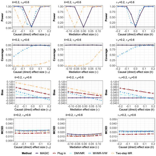
Figure 2: DGP 1-complete overlapping ($\mathcal{S}_{\mathtt{x}}^{*}=\mathcal{S}_{\mathtt{m}}^{*}$): Power, coverage, bias, and MCSD of MAGIC, Plug-in estimator, MVMR-IVW, DMVMR, and Two-step MR. First and second columns are computed under $\theta=0.2,\tau_{X}=0.6$, $\pi_{\mathtt{x}}=\pi_{\delta}=0.01$, and $\varepsilon_{\mathtt{x}}^{2}=1\times 10^{-4}$, $\varepsilon_{\delta}^{2}=5\times 10^{-5}$, that is for the second row, $\tau\in\{-0.12,-0.09,-0.06,-0.03,0,0.03,0.06,0.09,0.12\}$. The third column is computed when $\tau_{Y}=0.2$ and $\tau_{X}=0.6$. As two-step MR does not estimate $\theta$, it is not contained in the third row.

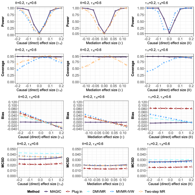
Figure 3: DGP 3(i) ($\mathcal{S}_{\mathtt{x}}^{*}\cap\mathcal{S}_{\delta}^{*}=\emptyset$): Power, coverage, bias, and MCSD of MAGIC, Plug-in estimator, MVMR-IVW, DMVMR, and Two-step MR. First and second columns are computed under $\theta=0.2,\tau_{X}=0.6$, $\pi_{\mathtt{x}}=\pi_{\delta}=0.01$, and $\varepsilon_{\mathtt{x}}^{2}=1\times 10^{-4}$, $\varepsilon_{\delta}^{2}=5\times 10^{-5}$, that is for the second row, $\tau\in\{-0.12,-0.09,-0.06,-0.03,0,0.03,0.06,0.09,0.12\}$.The third column is computed when $\tau_{Y}=0.2$ and $\tau_{X}=0.6$. As two-step MR does not estimate $\theta$, it is not contained in the third row.

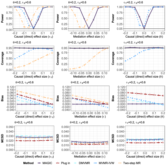
Figure 4: DGP 3(ii) ($|\mathcal{S}_{\mathtt{x}}^{*}\cap\mathcal{S}_{\delta}^{*}|=|\mathcal{S}_{\mathtt{x}}^{*}|/2$): Power, coverage, bias, and MCSD of MAGIC, Plug-in estimator, MVMR-IVW, DMVMR, and Two-step MR. First and second columns are computed under $\theta=0.2,\tau_{X}=0.6$, $\pi_{\mathtt{x}}=\pi_{\delta}=0.01$, and $\varepsilon_{\mathtt{x}}^{2}=1\times 10^{-4}$, $\varepsilon_{\delta}^{2}=5\times 10^{-5}$, that is for the second row, $\tau\in\{-0.12,-0.09,-0.06,-0.03,0,0.03,0.06,0.09,0.12\}$. The third column is computed when $\tau_{Y}=0.2$ and $\tau_{X}=0.6$. As two-step MR does not estimate $\theta$, it is not contained in the third row.

	${|\mathcal{S}_{\mathtt{x}}^{*}\setminus\mathcal{S}_{\mathtt{m}}^{*}|}/{|\mathcal{S}_{\mathtt{m}}^{*}\setminus\mathcal{S}_{\mathtt{x}}^{*}|}=0.1$		${|\mathcal{S}_{\mathtt{x}}^{*}\setminus\mathcal{S}_{\mathtt{m}}^{*}|}/{|\mathcal{S}_{\mathtt{m}}^{*}\setminus\mathcal{S}_{\mathtt{x}}^{*}|}=1$		${|\mathcal{S}_{\mathtt{x}}^{*}\setminus\mathcal{S}_{\mathtt{m}}^{*}|}/{|\mathcal{S}_{\mathtt{m}}^{*}\setminus\mathcal{S}_{\mathtt{x}}^{*}|}=3$
	DMVMR∗	MAGIC∗	DMVMR∗	MAGIC∗	DMVMR∗	MAGIC∗
$\pi_{{\mathtt{x}}\setminus{\mathtt{m}}}=\pi_{{\mathtt{m}}\setminus{\mathtt{x}}}=\pi_{{\mathtt{x}}\cap{\mathtt{m}}}=0.0005,\varepsilon_{\mathtt{x}}^{2}=5\times 10^{-5},\varepsilon_{\delta}^{2}=5\times 10^{-5}$
$\widehat{\theta}$	0.076	0.055	0.057	0.054	0.059	0.058
$\widehat{\tau}_{Y}$	0.022	0.022	0.052	0.049	0.062	0.058
$\pi_{{\mathtt{x}}\setminus{\mathtt{m}}}=\pi_{{\mathtt{m}}\setminus{\mathtt{x}}}=\pi_{{\mathtt{x}}\cap{\mathtt{m}}}=0.0005,\varepsilon_{\mathtt{x}}^{2}=5\times 10^{-5},\varepsilon_{\delta}^{2}=1\times 10^{-4}$
$\widehat{\theta}$	0.075	0.053	0.056	0.053	0.056	0.055
$\widehat{\tau}_{Y}$	0.015	0.015	0.035	0.034	0.044	0.043
$\pi_{{\mathtt{x}}\setminus{\mathtt{m}}}=\pi_{{\mathtt{m}}\setminus{\mathtt{x}}}=\pi_{{\mathtt{x}}\cap{\mathtt{m}}}=0.0005,\varepsilon_{\mathtt{x}}^{2}=5\times 10^{-5},\varepsilon_{\delta}^{2}=3\times 10^{-4}$
$\widehat{\theta}$	0.073	0.050	0.057	0.054	0.055	0.054
$\widehat{\tau}_{Y}$	0.010	0.010	0.020	0.020	0.024	0.024
$\pi_{{\mathtt{x}}\setminus{\mathtt{m}}}=\pi_{{\mathtt{m}}\setminus{\mathtt{x}}}=\pi_{{\mathtt{x}}\cap{\mathtt{m}}}=0.001,\varepsilon_{\mathtt{x}}^{2}=5\times 10^{-5},\varepsilon_{\delta}^{2}=1\times 10^{-4}$
$\widehat{\theta}$	0.050	0.037	0.039	0.036	0.039	0.038
$\widehat{\tau}_{Y}$	0.010	0.010	0.025	0.024	0.031	0.029
$\pi_{{\mathtt{x}}\setminus{\mathtt{m}}}=\pi_{{\mathtt{m}}\setminus{\mathtt{x}}}=\pi_{{\mathtt{x}}\cap{\mathtt{m}}}=0.001,\varepsilon_{\mathtt{x}}^{2}=5\times 10^{-5},\varepsilon_{\delta}^{2}=3\times 10^{-4}$
$\widehat{\theta}$	0.052	0.037	0.038	0.036	0.039	0.038
$\widehat{\tau}_{Y}$	0.006	0.006	0.013	0.013	0.016	0.016
$\pi_{{\mathtt{x}}\setminus{\mathtt{m}}}=\pi_{{\mathtt{m}}\setminus{\mathtt{x}}}=\pi_{{\mathtt{x}}\cap{\mathtt{m}}}=0.002,\varepsilon_{\mathtt{x}}^{2}=5\times 10^{-5},\varepsilon_{\delta}^{2}=1\times 10^{-4}$
$\widehat{\theta}$	0.035	0.025	0.027	0.026	0.028	0.027
$\widehat{\tau}_{Y}$	0.007	0.007	0.018	0.018	0.022	0.021
$\pi_{{\mathtt{x}}\setminus{\mathtt{m}}}=\pi_{{\mathtt{m}}\setminus{\mathtt{x}}}=\pi_{{\mathtt{x}}\cap{\mathtt{m}}}=0.002,\varepsilon_{\mathtt{x}}^{2}=5\times 10^{-5},\varepsilon_{\delta}^{2}=3\times 10^{-4}$
$\widehat{\theta}$	0.035	0.025	0.027	0.025	0.026	0.026
$\widehat{\tau}_{Y}$	0.004	0.004	0.010	0.010	0.012	0.012

Table 3: MCSD under different simulation designs and parameter settings. The true value of $(\theta,\tau_{Y},\tau_{X})=(0.2,0.2,0.6)$. MAGIC^∗ is the MAGIC estimator under the oracle scenario, and DMVMR^∗ is DMVMR under the oracle scenario. The total number of SNPs is 100,000. Here $\pi_{{\mathtt{x}}\setminus{\mathtt{m}}}$ is the proportion of SNPs that are only associated with $X$, $\pi_{{\mathtt{m}}\setminus{\mathtt{x}}}$ is the proportion of SNPs that are only associated with $M$, $\pi_{{\mathtt{x}}\cap{\mathtt{m}}}$ is the proportion of SNPs that are associated with both $X$ and $M$.

6 Real data analysis

Cardiovascular diseases (CVD) remain the leading global cause of death (Smith Jr et al., 2012), with a high body-mass index (BMI) recognized as an important risk factor (Tsao et al., 2022). However, the efficacy of current behavioral weight management interventions remains limited to the short term, and many weight loss medications, including recently approved ones, either lack long-lasting benefits or pose safety concerns (Tak and Lee, 2021; Myers-Ingram et al., 2023). By contrast, there are many effective clinical and public health interventions available to control cholesterol levels, blood pressure, and fasting glucose levels (Finucane et al., 2011). This situation has sparked growing interest in identifying metabolic factors that mediate between high BMI and cardiovascular disease, with the ultimate goal of targeting these metabolic factors to reduce the risk of CVD. While several metabolic factors that mediate the adverse effects of high BMI on cardiovascular diseases development have been identified (Lu et al., 2015), most of these findings are from traditional observational studies, potentially suffering from unmeasured confounding issues (Richiardi et al., 2013).

In this context, to identify metabolic factors that mediate the relationship between high BMI and cardiovascular diseases, we conduct mediation analysis with Mendelian randomization using GWAS summary data from the IEU OpenGWAS project (Lyon et al., 2021) and MEGASTROKE consortium (Malik et al., 2018). The exposure we consider include BMI, indicator of obesity (BMI $\geq 30\text{kg}/\text{m}^{2}$), and waist-to-hip ratio (WHR). Our investigation focuses on two major cardiovascular diseases: coronary artery disease (CAD) and stroke. For potential mediators, we consider modifiable metabolic factors such as lipids (hypercholesterolaemia, low-density lipoprotein cholesterol (LDL), high-density lipoprotein cholesterol (HDL)), blood pressure (systolic blood pressure (SBP), diastolic blood pressure (DBP)), and blood glucose (fasting glucose), along with negative control factors (hair color before graying). Detailed data information is summarized in Supplementary Material Section 8.5.

As a data pre-processing step, before conducting IV selection, we harmonize the exposure, mediator, and outcome GWAS data following the procedure detailed in Supplementary Material Section 8.1. Note that similar to the previous section, the IV selection procedure of MAGIC is different from the existing MR-based mediation analysis methods. Other than selecting relevant IVs, we also conduct clumping to remove the correlation between different IVs; see Supplementary Material Section 8.1 for implementation details.

Metabolic Mediators
Mediators	Pure hypercholes- -terolemia	LDL	HDL	SBP	DBP	Fasting Glu
BMI$\rightarrow$ Mediator $\rightarrow$ CAD
MAGIC	0.000	0.075	0.000	0.000	0.000	0.783
Two-step MR	0.008	0.056	0.000	0.004	0.064	0.079
WHR $\rightarrow$ Mediator $\rightarrow$ CAD
MAGIC	0.050	0.494	0.050	0.532	0.050	0.532
Two-step MR	0.024	0.999	0.106	0.198	0.064	0.214

Table 4: This table contains BH adjusted $p$-values for the mediation effects obtained from MAGIC and the two-step MR.

Given we have multiple mediators under consideration, we report Benjamini-Hochberg (BH) adjusted $p$-values (Benjamini and Hochberg, 1995) in Table 4. There, we compare the results provided by MAGIC and the two-step MR. We exclude MVMR-IVW from this comparison due to its inability to provide valid statistical inferences for mediation effects, as outlined in Table 2. Our results showcase that MAGIC successfully identifies DBP as a significant mediator in two pathways: (i) BMI$\rightarrow$DBP$\rightarrow$CAD, and (ii) WHR$\rightarrow$DBP$\rightarrow$CAD, and identifies HDL as a significant mediator in the pathway WHR$\rightarrow$HDL$\rightarrow$CAD. Existing literature provided some supportive evidence of these pathways. For example, both DBP and SBP’s role in mediating the risk of obesity to both CAD and stroke is well-established and the treatment of blood pressure has served as a main prevention and intervention therapy for CVD (Zang et al., 2022; McMackin et al., 2007; Ovbiagele et al., 2011; MacMahon et al., 1990). It has also been found that HDL is a marker and a mediator of CAD by removing overloaded cholesterol from cells in the artery wall and exerting anti-inflammatory effects (Heinecke, 2009). In contrast, the two-step MR fails to identify these significant mediators, suggesting that MAGIC may have a higher detection power than the two-step MR approach.

Additional results for other potential mediators including MVMR methods are provided in Section 8.2-8.4 in the Supplementary Material and are omitted in the main manuscript due to space limit.

7 Conclusion

In this manuscript, we introduced a novel mediation analysis framework employing Mendelian randomization with summary data. Our framework efficiently integrates information from three GWAS with carefully crafted estimating equations, leading to accurate direct and mediation effect estimation with enhanced statistical efficiency. In addition, the proposed method is immune to the winner’s/loser’s curse, corrects the measurement error bias, and remains valid even when instrument selection is imperfect. We provided rigorous statistical guarantees, including a joint asymptotic normality characterization of the estimated direct and mediation effects. We further demonstrated the construction of valid standard errors. We also discussed the potential efficiency gains of our approach relative to the debiased multivariable Mendelian Randomization in an oracle setting.

Supplementary Material

The Supplementary Material contains auxiliary lemmas, additional theoretical results, simulation evidence, additional real data analysis and all proofs.

References

• (1)
• Benjamini and Hochberg (1995) Benjamini, Y. and Hochberg, Y. (1995). “Controlling the false discovery rate: a practical and powerful approach to multiple testing,” Journal of the Royal Statistical Society: Series B, 57(1), 289–300.
• Bowden et al. (2015) Bowden, J., Davey Smith, G., and Burgess, S. (2015). “Mendelian randomization with invalid instruments: effect estimation and bias detection through Egger regression,” International Journal of Epidemiology, 44(2), 512–525.
• Bowden et al. (2016) Bowden, J., Del Greco M, F., Minelli, C., Davey Smith, G., Sheehan, N. A., and Thompson, J. R. (2016). “Assessing the suitability of summary data for two-sample Mendelian randomization analyses using MR-Egger regression: the role of the I2 statistic,” International Journal of Epidemiology, 45(6), 1961–1974.
• Bowden et al. (2019) Bowden, J., Del Greco M, F., Minelli, C., Zhao, Q., Lawlor, D. A., Sheehan, N. A. et al. (2019). “Improving the accuracy of two-sample summary-data Mendelian randomization: moving beyond the NOME assumption,” International Journal of Epidemiology, 48(3), 728–742.
• Burgess et al. (2013) Burgess, S., Butterworth, A., and Thompson, S. G. (2013). “Mendelian randomization analysis with multiple genetic variants using summarized data,” Genetic Epidemiology, 37(7), 658–665.
• Burgess et al. (2014) Burgess, S., Daniel, R. M., Butterworth, A. S., Thompson, S. G., and the EPIC-InterAct Consortium (2014). “Network Mendelian randomization: using genetic variants as instrumental variables to investigate mediation in causal pathways,” International Journal of Epidemiology, 44(2), 484–495.
• Burgess and Thompson (2015) Burgess, S. and Thompson, S. G. (2015). “Multivariable Mendelian randomization: the use of pleiotropic genetic variants to estimate causal effects,” American Journal of Epidemiology, 181(4), 251–260.
• Carter et al. (2021) Carter, A. R., Sanderson, E., Hammerton, G., Richmond, R. C., Davey Smith, G., Heron, J. et al. (2021). “Mendelian randomisation for mediation analysis: current methods and challenges for implementation,” European Journal of Epidemiology, 36(5), 465–478.
• Evans and Davey Smith (2015) Evans, D. M. and Davey Smith, G. (2015). “Mendelian randomization: new applications in the coming age of hypothesis-free causality,” Annual Review of Genomics and Human Genetics, 16, 327–350.
• Finucane et al. (2011) Finucane, M. M., Stevens, G. A., Cowan, M. J., Danaei, G., Lin, J. K., Paciorek, C. J. et al. (2011). “National, regional, and global trends in body-mass index since 1980: systematic analysis of health examination surveys and epidemiological studies with 960 country-years and 9.1 million participants,” The Lancet, 377(9765), 557–567.
• Gkatzionis and Burgess (2019) Gkatzionis, A. and Burgess, S. (2019). “Contextualizing selection bias in Mendelian randomization: how bad is it likely to be?” International Journal of Epidemiology, 48(3), 691–701.
• Grant and Burgess (2021) Grant, A. J. and Burgess, S. (2021). “Pleiotropy robust methods for multivariable Mendelian randomization,” Statistics in Medicine, 40(26), 5813–5830.
• Heinecke (2009) Heinecke, J. W. (2009). “The HDL proteome: a marker–and perhaps mediator–of coronary artery disease,” Journal of Lipid Research, 50(Suppl), S167–S171.
• Jiang and Ding (2020) Jiang, Z. and Ding, P. (2020). “Measurement errors in the binary instrumental variable model,” Biometrika, 107(1), 238–245.
• Lu et al. (2015) Lu, Y., Hajifathalian, K., Rimm, E. B., Ezzati, M., and Danaei, G. (2015). “Mediators of the effect of body mass index on coronary heart disease: decomposing direct and indirect effects,” Epidemiology, 26(2), 153–162.
• Lyon et al. (2021) Lyon, M. S., Andrews, S. J., Elsworth, B., Gaunt, T. R., Hemani, G., and Marcora, E. (2021). “The variant call format provides efficient and robust storage of GWAS summary statistics,” Genome Biology, 22(32), 1–10.
• Ma et al. (2023) Ma, X., Wang, J., and Wu, C. (2023). “Breaking the winner’s curse in Mendelian randomization: rerandomized inverse variance weighted estimator,” Annals of Statistics, 51(1), 211–232.
• MacMahon et al. (1990) MacMahon, S., Peto, R., Collins, R., Godwin, J., Cutler, J., Sorlie, P. et al. (1990). “Blood pressure, stroke, and coronary heart disease: part 1, prolonged differences in blood pressure: prospective observational studies corrected for the regression dilution bias,” The Lancet, 335(8692), 765–774.
• Malik et al. (2018) Malik, R., Chauhan, G., Traylor, M., Sargurupremraj, M., Okada, Y., Mishra, A. et al. (2018). “Multiancestry genome-wide association study of 520,000 subjects identifies 32 loci associated with stroke and stroke subtypes,” Nature Genetics, 50(4), 524–537.
• McMackin et al. (2007) McMackin, C. J., Widlansky, M. E., Hamburg, N. M., Huang, A. L., Weller, S., Holbrook, M. et al. (2007). “Effect of combined treatment with $\alpha$-lipoic acid and acetyl-l-carnitine on vascular function and blood pressure in patients with coronary artery disease,” Journal of Clinical Hypertension, 9(4), 249–255.
• Myers-Ingram et al. (2023) Myers-Ingram, R., Sampford, J., Milton-Cole, R., and Jones, G. D. (2023). “Effectiveness of eHealth weight management interventions in overweight and obese adults from low socioeconomic groups: a systematic review,” Systematic Reviews, 12(1), 1–12.
• Ovbiagele et al. (2011) Ovbiagele, B., Diener, H.-C., Yusuf, S., Martin, R. H., Cotton, D., Vinisko, R. et al. (2011). “Level of systolic blood pressure within the normal range and risk of recurrent stroke,” JAMA, 306(19), 2137–2144.
• Relton and Davey Smith (2012) Relton, C. L. and Davey Smith, G. (2012). “Two-step epigenetic Mendelian randomization: a strategy for establishing the causal role of epigenetic processes in pathways to disease,” International Journal of Epidemiology, 41(1), 161–176.
• Richiardi et al. (2013) Richiardi, L., Bellocco, R., and Zugna, D. (2013). “Mediation analysis in epidemiology: methods, interpretation and bias,” International Journal of Epidemiology, 42(5), 1511–1519.
• Robertson et al. (2016) Robertson, D. S., Prevost, A. T., and Bowden, J. (2016). “Accounting for selection and correlation in the analysis of two-stage genome-wide association studies,” Biostatistics, 17(4), 634–49.
• Sadreev et al. (2021) Sadreev, I. I., Elsworth, B. L., Mitchell, R. E., Paternoster, L., Sanderson, E., Davies, N. M. et al. (2021). “Navigating sample overlap, winner’s curse and weak instrument bias in Mendelian randomization studies using the UK Biobank,” MedRxiv.
• Sanderson (2021) Sanderson, E. (2021). “Multivariable Mendelian randomization and mediation,” Cold Spring Harbor Perspectives in Medicine, v.11(2), a038984.
• Sanderson et al. (2018) Sanderson, E., Davey Smith, G., Windmeijer, F., and Bowden, J. (2018). “An examination of multivariable Mendelian randomization in the single-sample and two-sample summary data settings,” International Journal of Epidemiology, 48(3), 713–727.
• Sanderson et al. (2021) Sanderson, E., Spiller, W., and Bowden, J. (2021). “Testing and correcting for weak and pleiotropic instruments in two-sample multivariable Mendelian randomization,” Statistics in Medicine, 40(25), 5434–5452.
• Smith (1981) Smith, J. L. (1981). “Non-aggressive bidding behavior and the “winner’s curse”,” Economic Inquiry, 19(3), 380–388.
• Smith Jr et al. (2012) Smith Jr, S. C., Collins, A., Ferrari, R., Holmes Jr, D. R., Logstrup, S., McGhie, D. V. et al. (2012). “Our time: a call to save preventable death from cardiovascular disease (heart disease and stroke),” Circulation, 126(23), 2769–2775.
• Sollis et al. (2023) Sollis, E., Mosaku, A., Abid, A., Buniello, A., Cerezo, M., Gil, L. et al. (2023). “The NHGRI-EBI GWAS Catalog: knowledgebase and deposition resource,” Nucleic Acids Research, 51(D1), D977–D985.
• Tak and Lee (2021) Tak, Y. J. and Lee, S. Y. (2021). “Long-term efficacy and safety of anti-obesity treatment: where do we stand?” Current Obesity Reports, 10, 14–30.
• Tsao et al. (2022) Tsao, C. W., Aday, A. W., Almarzooq, Z. I., Alonso, A., Beaton, A. Z., Bittencourt, M. S. et al. (2022). “Heart disease and stroke statistics—2022 update: a report from the American Heart Association,” Circulation, 145(8), e153–e639.
• Ye et al. (2021) Ye, T., Shao, J., and Kang, H. (2021). “Debiased inverse-variance weighted estimator in two-sample summary-data Mendelian randomization,” Annals of Statistics, 49(4), 2079–2100.
• Zang et al. (2022) Zang, J., Liang, J., Zhuang, X., Zhang, S., Liao, X., and Wu, G. (2022). “Intensive blood pressure treatment in coronary artery disease: implications from the Systolic Blood Pressure Intervention Trial (SPRINT),” Journal of Human Hypertension, 36(1), 86–94.
• Zhao et al. (2020) Zhao, Q., Wang, J., Hemani, G., Bowden, J., and Small, D. S. (2020). “Statistical inference in two-sample summary-data Mendelian randomization using robust adjusted profile score,” Annals of Statistics, 48(3), 1742–1769.