Bayes-Optimal Unsupervised Learning for Channel Estimation in Near-Field Holographic MIMO

Abstract

Holographic MIMO (HMIMO) is being increasingly recognized as a key enabling technology for 6G wireless systems through the deployment of an extremely large number of antennas within a compact space to fully exploit the potentials of the electromagnetic (EM) channel. Nevertheless, the benefits of HMIMO systems cannot be fully unleashed without an efficient means to estimate the high-dimensional channel, whose distribution becomes increasingly complicated due to the accessibility of the near-field region. In this paper, we address the fundamental challenge of designing a low-complexity Bayes-optimal channel estimator in near-field HMIMO systems operating in unknown EM environments. The core idea is to estimate the HMIMO channels solely based on the Stein’s score function of the received pilot signals and an estimated noise level, without relying on priors or supervision that is not feasible in practical deployment. A neural network is trained with the unsupervised denoising score matching objective to learn the parameterized score function. Meanwhile, a principal component analysis (PCA)-based algorithm is proposed to estimate the noise level leveraging the low-rank near-field spatial correlation. Building upon these techniques, we develop a Bayes-optimal score-based channel estimator for fully-digital HMIMO transceivers in a closed form. The optimal score-based estimator is also extended to hybrid analog-digital HMIMO systems by incorporating it into a low-complexity message passing algorithm. The (quasi-) Bayes-optimality of the proposed estimators is validated both in theory and by extensive simulation results. In addition to optimality, it is shown that our proposal is robust to various mismatches and can quickly adapt to dynamic EM environments in an online manner thanks to its unsupervised nature, demonstrating its potential in real-world deployment.

I Introduction

With an ultra-massive number of antennas closely packed in a compact space, holographic MIMO (HMIMO) is envisioned as a promising next-generation multi-antenna technology to enable an unprecedentedly high degree of spectral and energy efficiency [2]. Extensive research efforts have been dedicated to many different aspects of HMIMO systems, such as channel measurement and modeling [2, 3, 4, 5, 6], beamforming methods [7, 8, 9], positioning and sensing [10, 11], and integrated sensing and communications [12], etc. Nevertheless, one fundamental problem is that, the promised gains brought by HMIMO can hardly be realized without an efficient means to estimate the extremely high-dimensional channel.

The challenges to estimate the HMIMO channel are mainly three-fold [13]. The first challenge arises from the complicated and dynamic channel distributions. The extremely large-scale array significantly expands the near-field region with spherical wavefront, which greatly complicates the channel distributions and enlarges the codebook size to sparsify the channel [14]. Also, since HMIMO systems often operate at higher frequency bands, they are vulnerable to various types of blockage and movement, which can easily shift the channel distributions in a dynamic manner. Second, priors or a supervised dataset are difficult to obtain. Existing estimators either utilized the prior knowledge, e.g., sparsity in some transform domain, or a large supervised channel dataset, to enhance the estimation accuracy. Nevertheless, both of them require tedious, if not prohibitive, efforts to realize in practice, considering the enormous system scale and the complicated channel distributions in the near-field HMIMO systems. The computational complexity poses the third challenge. The scale of near-field HMIMO systems prohibits the use of classical Bayes-optimal channel estimators which include complicated matrix inversion, and calls for low-complexity alternatives.

I-A Related Works

The simplest approach to estimating the channel is the least squares (LS) method [15], which offers reasonable performance in fully-digital systems but suffers from a high pilot overhead in hybrid analog-digital systems. To enhance the performance, the regularized LS estimators prevail, which, in addition to the LS objective, minimize an extra regularization term to enforce the channel to follow the prior knowledge of its characteristics, e.g., sparsity [16] or low-rankness [17]. By contrast, the Bayesian point of view instead believes that the channels should follow a prior distribution, and focuses on optimizing the maximum a posteriori (MAP) or the minimum mean-square-error (MMSE) objectives [18]. Both the regularization-based and Bayesian perspectives stress the availability of a proper prior. Nevertheless, finding such a prior may be difficult in practice as the HMIMO channels have become increasingly complicated, e.g., with the near-field [14] and hybrid-field effects [19]. Simply resorting to the classical angular domain sparsity or the priors based on some simple mixture distributions can no longer offer competitive accuracy.

Deep learning (DL)-based approaches then emerge as a potential paradigm that attempts to learn the priors from a large volume of data instead of relying on hand-crafted designs [20]. As a result, data is fundamental to DL-based methods. Depending on how the data are leveraged, DL methods can be categorized as supervised, unsupervised, and generative approaches. As for the channel estimation problem, supervised learning refers to those that require a paired dataset of the received pilot signals $\mathbf{y}$ and the channel $\mathbf{h}$, i.e., $(\mathbf{y},\mathbf{h})$, in order to implicitly exploit the prior, while the generative learning requires a dataset of $\mathbf{h}$ to explicitly model the prior distribution [21]. However, both supervised and generative learning requires a dataset involving the ground-truth channel $\mathbf{h}$, which, in practice, cannot be easily acquired without a competitive channel estimator. This brings about a chicken-and-egg dilemma: To train competitive models we need to prepare a dataset of ground-truth channels, but such a channel dataset comes from nowhere. To tackle the dilemma, unsupervised learning is an ideal candidate as it only requires a dataset of the received pilots $\mathbf{y}$, which can be readily obtained in abundant volume. Nevertheless, existing unsupervised channel estimators generally suffer from sub-optimal accuracy. In [22], the authors proposed to train a multi-layer perceptron (MLP)-based neural network to minimize online loss functions based on the LS and the nuclear-norm-based regularizer, respectively. This is, essentially, training a neural network-based solver for the regularization-based channel estimator, whose performance is hence still subject to the hand-cracfted regularizer. Results therein show a large performance gap compared to supervised learning. In [23, 24], the authors proposed to minimize the Stein’s unbiased risk estimator (SURE) objective as a surrogate to the mean-square-error (MSE) loss in order to approach the accuracy of supervised learning. Nevertheless, the SURE loss involves a Monte-Carlo approximation, which will degrade the accuracy of the trained estimator and increase its bias. Hence, the performance is still inferior to supervised training, let alone the oracle performance bound.

As a golden standard, the MMSE estimator can achieve the Bayes-optimal accuracy in terms of MSE. Nevertheless, as mentioned in the above discussions, its implementation requires either a perfect knowledge of the prior distribution [4, 25], or learning such a distribution from a substantial number of ground-truth channels [19, 13], both of which are difficult, if not impossible, to realize in near-field HMIMO systems. In addition, computational complexity is again a significant issue. Even the linear MMSE (LMMSE) estimator still contains a general matrix inverse that consumes a significant amount of computational budget [26]. The existing works on HMIMO channel estimation mainly focused on the low-complexity alternatives to the MMSE estimator. In [4], a subspace-based channel estimation algorithm was proposed, in which the low-rank property of the HMIMO spatial correlation was exploited without full knowledge of the spatial correlation. In [27], a discrete Fourier transform (DFT)-based HMIMO channel estimator was proposed based on a circulant matrix-based approximation of the spatial correlation matrix. Nevertheless, such an algorithm was limited to the uniform linear array (ULA)-based HMIMO systems, and cannot be extended to more general antenna array geometries. In [28], angular domain channel sparsity was exploited for the design of compressed sensing (CS)-based channel estimators in holographic reconfigurable intelligent surface (RIS)-aided wireless systems. Nevertheless, such a nice property dose not hold in the considered near-field region. In [25], a concise tutorial of HMIMO channel modeling and estimation was presented. Even though the aforementioned estimators significantly outperform the conventional LS scheme, there still exists quite a large gap from that of the Bayes-optimal MMSE estimator.

The lack of the prior distribution and the supervised dataset hinders existing algorithms from achieving the Bayes-optimal estimator of the near-field HMIMO channel. Thus, we naturally wonder if it is possible to devise advanced unsupervised DL-based algorithms to fill this important research gap.

I-B Contributions

The goal of this work is to establish an efficient and Bayes-optimal channel estimator for near-field HMIMO systems that operates in an arbitrary unknown EM environment, circumventing the need of priors or supervision. The main contributions are summarized as follows.

• We introduce an unsupervised DL framework that validates the feasibility of establishing Bayes-optimal channel estimators solely based on the Stein’s score function of the received pilot signals and the estimated noise level.

• We then devise practical algorithms to obtain the two key ingredients of the unsupervised Bayes-optimal estimator, i.e., the score function and the noise level. For the former, we propose to train a neural network-based parameterized score function with the denoising score matching loss. As for the latter, we exploit the low-rankness of the near-field spatial correlation to build a principal component analysis (PCA)-based noise level estimator. The theoretical underpinnings are discussed along with the algorithms.

• We propose score-based channel estimators for near-field HMIMO systems with both the fully-digital and hybrid analog-digital architectures. For fully-digital transceivers, the Bayes-optimal estimator is as simple as a sum of the received pilot signals and the rescaled score function by the estimated noise level. As for the hybrid analog-digital architecture, we insert the proposed score-based estimator into iterative message passing algorithms, and propose an efficient technique to reduce their complexity. A complexity analysis shows that the algorithms in both setups are only dominated by the matrix-vector product.

• Extensive numerical results demonstrate that the proposed score-based estimator is indeed quasi-optimal when compared to the oracle performance bound. In addition, the robustness and the generalization capability are validated in different system configurations. Furthermore, thanks to the unsupervised nature, the proposed estimator can automatically adapt to dynamic environments with varying channel distributions, which justifies its practical value.

I-C Paper Organization and Notation

The remaining parts of the article are organized as follows. In Section II, we introduce the statistical channel model and the system model for near-field HMIMO systems. In Section III, we first discuss the general framework and the two core techniques of the score-based estimator, i.e., the unsupervised learning of the score function and the PCA-based noise level estimation. Then, in Section IV, we respectively present the algorithms for the fully-digital, as well as the hybrid analog-digital systems. In Section V, extensive simulation results are presented to illustrate the advantages of our proposal in terms of performance, generalization, and robustness. In Section VI, we conclude the paper and discuss future directions.

Notation: $a$ is a scalar. $\text{tr}(\mathbf{a})$, $\|\mathbf{a}\|$, and $\mathbf{a}(n)$ are the trace, the $\ell_{2}$-norm, and the $n$-th entry of a vector $\mathbf{a}$, respectively. $\mathbf{A}^{T}$, $\mathbf{A}^{H}$, $\text{$\Re$}(\mathbf{A})$, $\Im(\mathbf{A})$, $\mathbf{A}(n,m)$ are the transpose, Hermitian, real part, imaginary part, and the $(n,m)$-th entry of a matrix $\mathbf{A}$, respectively. $\mathcal{CN}(\boldsymbol{\mu},\mathbf{R})$ and $\mathcal{N}(\boldsymbol{\mu},\mathbf{R})$ are the complex and the real Gaussian distributions with mean $\boldsymbol{\mu}$ and covariance $\mathbf{R}$, respectively. $\mathbf{I}$ is an identity matrix with appropriate size.

II HMIMO Channel and System Models

II-A Channel Model for Near-Field HMIMO

Consider the uplink of an HMIMO system where the base station (BS) is equipped with a uniform linear array (ULA) with thousands of compactly packed antennas with spacings $d_{a}$ being much smaller than half of the carrier wavelength $\lambda_{c}$, i.e., $d_{a}\ll\frac{\lambda_{c}}{2}$, as illustrated in Fig. 1. The BS is assumed to simultaneously serve multiple single-antenna users. We define a Cartesian coordinate system at the center of the ULA (i.e., the reference antenna), denoted by $\mathbf{w}_{0}$. Similarly, we denote the position of the $n$-th antenna as $\mathbf{w}_{n}$. The propagation characteristics of the channel differ in the near-field and far-field regions, whose boundary is determined by the Rayleigh distance $d_{\text{Rayleigh}}\triangleq\frac{2[(N-1)d_{a}]^{2}}{\lambda_{c}}$, where $N$ refers to the number of antennas. Due to the joint effect of the array aperture and the carrier wavelength, the near-field region is non-negligible in HMIMO systems, which, compared to the traditional far-field setup, is a paradigm shift that brings new degrees-of-freedom (DoFs) for both communications and sensing [10].

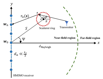
Figure 1: A ULA-shaped HMIMO BS in the cartesian coordinate system, where the transmitter and the scatterers locate in the near field of the HMIMO array.

When there are infinitely many multi-paths, it follows from the central limit theorem that the channel between the HMIMO and a particular user, i.e., $\mathbf{\bar{h}}\in\mathbb{C}^{N\times 1}$, can be modeled by the correlated Rayleigh fading as [4, 25, 29]

$$\mathbf{\bar{h}}\sim\mathcal{CN}(\mathbf{0},\mathbf{R}_{\text{NF}}),$$ (1)

which is solely determined by the spatial correlation $\mathbf{R}_{\text{NF}}\in\mathbb{C}^{N\times N}$, with subscript NF denoting the near-field. This model has been and still is the foundation of most theoretical research in HMIMO systems [2, 4]. It has been further established in [30] that, while the number of scatterers tends to infinity, the near-field spatial correlation for HMIMO has a generic integral expression, given by

$$\mathbf{R}_{\text{NF}}(n,m)=\beta_{0}\int_{\mathbf{s}\in\mathbf{S}}\frac{r_{0}^{2}(\mathbf{s})e^{-j\frac{2\pi}{\lambda_{c}}\left(r_{n}(\mathbf{s})-r_{m}(\mathbf{s})\right)}}{r_{n}(\mathbf{s})r_{m}(\mathbf{s})}f(\mathbf{s})\mathrm{d}\mathbf{s},$$ (2)

where $\beta_{0}$ denotes the average received power at the reference antenna, $\mathbf{s}\in\mathbf{S}$ denotes the position of a scatterer in the support of random scatterers $\mathbf{S}$, $r_{n}(\mathbf{s})\triangleq\|\mathbf{s}-\mathbf{w}_{n}\|$ refers to the distance between scatterer $\mathbf{s}$ and the $n$-th antenna element, and $f(\mathbf{s})$ is the probability density function (PDF) of the scatterer location, called the power location spectrum (PLS). The expression (2) holds true for any PLS $f(\mathbf{s})$.

To gain further insights, we consider a specific $f(\mathbf{s})$, named the generalized one-ring model, assuming that the scatterers are located on a ring whose center is freely positioned, as shown in Fig. 1. We denote the radius and the angular direction of the ring as $R\geq 0$ and $\Psi\in(-\frac{\pi}{2},\frac{\pi}{2})$, respectively. The coordinate of the ring center is given by $\mathbf{c}=[S\cos\Psi,S\sin\Psi]^{T}$, where $S\geq 0$ is the distance between the origin and the ring center. The location of a certain scatterer on the ring is then given by $\mathbf{s}=\mathbf{c}+[R\cos\phi,R\sin\phi]^{T}$, where $\phi\in[-\pi,\pi)$ is the angular position of the scatterer on the ring. We notice that in a certain EM environment in which $S$, $R$, and $\Psi$ are given, the distance $r_{n}(\mathbf{s})$ in (2) reduces to a function of $\phi$, given by

$$r_{n}(\phi)=\sqrt{(S\sin\Psi+R\sin\phi-nd_{a})^{2}+(S\cos\Psi+R\cos\phi)^{2}},$$ (3)

so as $f(\mathbf{s})$, which reduces to $f(\phi)$. Plugging (3) into (2), when $S\gg R$ is satisfied, the near-field spatial correlation $\mathbf{R}_{\text{NF}}$ can be approximately simplified as

$$\mathbf{R} {}_{\text{NF}}(n,m)$$ (4)

$$\thickapprox\beta_{0}\int_{-\pi}^{\pi}\frac{e^{-j\frac{2\pi}{\lambda_{c}}\left(R\left(\frac{b_{n}}{\sqrt{a_{n}}}-\frac{b_{m}}{\sqrt{a_{m}}}\right)+S\left(\sqrt{a_{n}}-\sqrt{a_{m}}\right)\right)}}{\sqrt{a_{n}a_{m}}}f(\phi)\mathrm{d}\phi,$$

according to [30, Lemma 2]. Here $a_{n}$ and $b_{n}$ are respectively defined as $a_{n}\triangleq(nd_{a}/S)^{2}-2(nd_{a}/S)+1$ and $b_{n}\triangleq\cos(\Psi-\phi)-(nd_{a}/S)\sin\phi$, while $a_{m}$ and $b_{m}$ are determined similarly. For the ease of simulations, we utilize the particular von-Mises distribution for $f(\phi)$ to model the scatterer distribution on the ring, given by [31]

$$f(\phi)=(2\pi I_{0}(\kappa))^{-1}e^{\kappa\cos(\phi-\mu)},$$ (5)

in which $I_{0}(\cdot)$ denotes the zeroth-order Bessel function of the first kind, while $\kappa\geq 0$ and $\mu\in[-\pi,\pi)$ are the two parameters determining the concentration and the mean of the distribution, respectively. The distribution is the circular analog of the normal distribution. When $\kappa$ is zero, the distribution is uniform, while when $\kappa$ is large, the distribution becomes concentrated about the angle $\mu$. After plugging (5) into (4), the integration can be computed numerically by Monte-Carlo methods to obtain the near-field spatial correlation $\mathbf{R}_{\text{NF}}$.

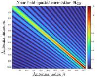
(a)

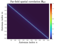
(b)

Figure 2: (a) The heat map of the near-field spatial correlation matrix, when the BS is equipped with a ULA with 1024 antennas that operates at a carrier frequency of $f_{c}=3.5$ GHz. Other parameters are $d=\frac{\lambda_{c}}{10}$, $S=20$ m, $R=3$ m, $\Psi=\frac{\pi}{3}$, $\mu=\frac{\pi}{4}$, and $\kappa=0$. (b) The heat map of the far-field spatial correlation in isotropic scattering environments, with the same carrier frequency and array configuration. The comparison reveals the difference between the far-field and the near-field spatial correlation matrices.

By contrast, the far-field spatial correlation $\mathbf{R}_{\text{FF}}\in\mathbb{C}^{N\times N}$ is characterized by the following integration [27, 30], i.e.,

$$\mathbf{R}_{\text{FF}}(n,m)=\beta_{0}\int_{-\pi}^{\pi}e^{-j\frac{2\pi}{\lambda_{c}}(m-n)d_{a}\sin\theta}f(\vartheta)\mathrm{d}\vartheta,$$ (6)

in which $\vartheta$ is the angle of arrival (AoA), and $f(\vartheta)$ is the power angular spectrum (PAS) characterizing the power distribution over different AoAs [30]. In particular, in isotropic scattering environments where the multi-paths are uniformly distributed, $\mathbf{R}_{\text{FF}}$ has a closed-form expression, i.e., [32]

$$\mathbf{R}_{\text{FF-iso}}(n,m)=\operatorname{sinc}\left(\frac{2\left\|\mathbf{w}_{n}-\mathbf{w}_{m}\right\|}{\lambda_{c}}\right).$$ (7)

Otherwise, in non-isotropic scattering environments, $\mathbf{R}_{\text{FF}}$ can also be obtained through numerical integration.

The differences between the near-field and the far-field spatial correlations are two-fold. First, $\mathbf{R}_{\text{FF}}$ is solely determined by the PAS, $f(\vartheta)$, whereas $\mathbf{R}_{\text{NF}}$ relies not only on the AoAs but also on the scatterers’ positions, denoted as the PLS, $f(\mathbf{s})$. Second, although $\mathbf{R}_{\text{FF}}$ exhibits spatial wide-sense stationarity, as evidenced by $\mathbf{R}_{\text{FF}}(n,m)$ being solely dependent on array index difference, $m-n$, this stationary characteristic does not generally apply to $\mathbf{R}_{\text{NF}}$. When $r(\mathbf{s})\gg Nd_{a},\forall\mathbf{s}\in\mathbf{S}$ holds true, the two expressions are approximately equal, i.e., $\mathbf{R}_{\text{NF}}\approx\mathbf{R}_{\text{FF}}$, but in other cases, the exact near-field correlation $\mathbf{R}_{\text{NF}}$ must be taken into account. For better illustration, we plot a visualized comparison of $\mathbf{R}_{\text{NF}}$ and $\mathbf{R}_{\text{FF}}$ in Fig. 2. It is observed that the element of the far-field spatial correlation $\mathbf{R}_{\text{FF}}(n,m)$ is solely determined by the index difference $n-m$, which is called the spatial stationarity property. By contrast, such a property does not hold for the near-field spatial correlation, whose element $\mathbf{R}_{\text{NF}}(n,m)$ depends explicitly on both indexes $n$ and $m$. Also, the near-field correlation $\mathbf{R}_{\text{NF}}$ results in a non-uniform average power distribution among the antennas.

II-B System Model for Near-Field HMIMO

We introduce the system model for the near-field HMIMO. We mainly consider two mainstream transceiver architectures, i.e., the fully-digital and the hybrid analog-digital ones [33]. We assume orthogonal pilots are utilized and hence focus on a specific user without loss of generality. In the uplink channel estimation, the user sends pilots to the BS for $K$ time slots. The received pilot signals, $\mathbf{\bar{y}}_{k}\in\mathbb{C}^{N_{\text{RF}}\times 1}$, at time slot $k$ is

$$\mathbf{\bar{y}}_{k}=\mathbf{W}_{k}^{H}(\bar{\mathbf{h}}s_{k}+\mathbf{\bar{n}}_{k}),$$ (8)

where $\mathbf{W}_{k}\in\mathbb{C}^{N\times N_{\text{RF}}}$ is the pilot combining matrix, $s_{k}=1$ is the pilot symbol, and $\mathbf{\bar{n}}_{k}\sim\mathcal{CN}(\mathbf{0},\sigma_{\mathbf{\bar{n}}}^{2}\mathbf{I})$ refers to the additive white Gaussian noise. After $K$ time slots of pilot transmission, the received pilot signals are $\bar{\mathbf{y}}=\mathbf{\bar{M}}\mathbf{\bar{h}}+\mathbf{\bar{n}}$, in which $\bar{\text{$\mathbf{M}$}}=[\mathbf{W}_{1}^{T},\mathbf{W}_{2}^{T},\ldots,\mathbf{W}_{K}^{T}]^{T}\in\mathbb{C}^{KN_{\text{RF}}\times N}$, $\bar{\mathbf{y}}=[\mathbf{\bar{y}}_{1}^{T},\mathbf{\bar{y}}_{2}^{T},\ldots,\mathbf{\bar{y}}_{K}^{T}]^{T}\in\mathbb{C}^{KN_{\text{RF}}\times 1}$, and the noise $\mathbf{\bar{n}}$ is obtained similarly and whitened as [24]. In fully-digital HMIMO systems, the number of radio frequency chains is equal to that of antennas, i.e., $N_{\text{RF}}=N$. We may set the combiner as $\mathbf{W}_{k}=\mathbf{I}$, and the system model reduces to $\bar{\mathbf{y}}=\mathbf{\bar{h}}+\mathbf{\bar{n}}$ [4, 25, 27]. In contrast, in hybrid analog-digital systems, the pilot combing matrix is the product of an analog combiner $\mathbf{W}_{\text{RF},k}^{H}$ and a digital combiner $\mathbf{W}_{\text{BB},k}^{H}$, i.e., $\mathbf{W}_{k}^{H}=\mathbf{W}_{\text{RF},k}^{H}\mathbf{W}_{\text{BB},k}^{H}$. Notice that the combiners cannot be optimally tuned without knowledge of the channel. Without loss of generality, we consider an arbitrary scenario in which the digital combiner $\mathbf{W}_{\text{BB},k}^{H}$ is configured as identity, and the elements of the analog combiner $\mathbf{W}_{\text{RF},k}^{H}$ are randomly selected from one-bit quantized phase shifts for the energy efficiency considerations [19, 26]. The elements of $\bar{\text{$\mathbf{M}$}}$ follows the same distribution as $\mathbf{W}_{\text{RF},k}^{H}$, that is $(\bar{\text{$\mathbf{M}$}})_{i,j}\in\frac{1}{\sqrt{N/N_{\text{RF}}}}\{\pm 1\}$. As most of the existing deep learning libraries handle real-valued inputs, we transform the received pilot signals into a equivalent real-valued form,

$$\mathbf{y=\mathbf{Mh}+\mathbf{n}},$$ (9)

in which $\mathbf{M}=\text{blkdiag}(\Re(\mathbf{\bar{M}}),\Re(\mathbf{\bar{M}}))\in\mathbb{R}^{2KN_{\text{RF}}\times 2N}$, $\mathbf{y}=[\Re(\mathbf{\bar{y}})^{T},\Im(\mathbf{\bar{y}})^{T}]^{T}\in\mathbb{R}^{2KN_{\text{RF}}\times 1}$, and $\mathbf{n}=[\Re(\mathbf{\bar{n}})^{T},\Im(\mathbf{\bar{n}})^{T}]^{T}\sim\mathcal{N}(\mathbf{0},\sigma_{\mathbf{\mathbf{n}}}^{2}\mathbf{I})$ with $\sigma_{\mathbf{\mathbf{n}}}^{2}=\frac{1}{2}\sigma_{\mathbf{\bar{n}}}^{2}$.

Given the fact that $N_{\text{RF}}\ll N$ holds in hybrid analog-digital systems and a small pilot overhead $K$, the measurement matrix $\mathbf{M}$ is often a fat matrix with $KN_{\text{RF}}<N$. This means that the dimension of $\mathbf{y}$ is smaller than that of the channels $\mathbf{h}$, which renders channel estimation an under-determined problem with infinitely many possible solutions. This necessitates the use of the prior knowledge of the channel $\mathbf{h}$ in some forms to reach a high-quality solution. By contrast, since $N_{\text{RF}}=N$ in fully-digital transceivers, it is good enough to simply set $K=1$ in the channel estimation stage. In such a scenario, $\mathbf{M}$ is a square matrix, i.e., $\mathbf{M=I}$, and the system model becomes

$$\mathbf{y=\mathbf{h}+\mathbf{n}},$$ (10)

which reduces to a denoising problem. Nevertheless, to achieve competitive estimation performance, it is essential to leverage the prior of the channel $\mathbf{h}$, not to mention the Bayes-optimal MMSE estimator, which typically requires full knowledge of the prior distribution $p(\mathbf{h})$.

However, the grand challenge is that, we actually have very limited prior knowledge of the channel $\mathbf{h}$ in real environments, let alone characterizing its full prior distribution. As mentioned in Section I, previous works either attempt to adopt simplified priors, e.g., based on sparsity and low-rankness, or introduce the postulated ones, e.g., by using mixture distributions, which, however, can only characterize a limited aspects of the channel feature, and hence often result in sub-optimal performance. On the other hand, existing DL methods mostly rely on a supervised dataset of ground-truth channels $\mathbf{h}$, which are hardly available in practice. Hence, in the next section, we study how to achieve Bsyes-optimal channel estimation without priors or supervision, which is extremely important in practice.

III General Frameworks of the Score-Based Channel Estimator

In this section, we propose general frameworks and enabling techniques of the Bayes-optimal score-based channel estimator. We first consider the fully-digital transceivers and derive the closed-form expression of the Bayes-optimal channel estimator solely based on the received pilot signals $\mathbf{y}$. Next, we propose techniques to acquire the two crucial elements of the estimator, namely the score function and the noise level, based on score matching and PCA, respectively.

III-A Bridging MMSE Estimation with the Score Function

In this subsection, we first focus on the fully-digital system model, i.e., (10). Extension to hybrid analog-digital HMIMO systems will be presented in Section IV-B.

Our target is a Bayes-optimal channel estimator, $\mathbf{\hat{h}}=D(\mathbf{y})$, that minimizes the mean-square-error (MSE), i.e.,

$$\text{MSE}\triangleq\text{$\mathbb{E}(\|\mathbf{h}-\hat{\mathbf{h}}\|^{2}|\mathbf{y})=\int\|\mathbf{h}-\mathbf{\hat{h}}\|^{2}p(\mathbf{h}|\mathbf{y})d\mathbf{h}$},$$ (11)

where the expectation above is taken with respect to (w.r.t.) the unknown channel $\mathbf{h}$, while $p(\mathbf{h}|\mathbf{y})$ is the posterior density. Taking the derivative of the above equation w.r.t. $\hat{\mathbf{h}}$ and nulling it, we reach the Bayes-optimal, i.e., minimum MSE (MMSE), channel estimator, given by

$$\hat{\mathbf{h}}_{\text{MMSE}} =\mathbb{E}(\mathbf{h}|\mathbf{y})=\int\mathbf{h}p(\mathbf{h}|\mathbf{y})d\mathbf{h}=\int\mathbf{h}\frac{p(\mathbf{h},\mathbf{y})}{p(\mathbf{y})}d\mathbf{h},$$ (12)

where $p(\mathbf{h},\mathbf{y})$ is the joint density, and $p(\mathbf{y})$ is the measurement density obtained via marginalization, i.e.,

$$p(\mathbf{y}) =\int p(\mathbf{h},\mathbf{y})d\mathbf{h}=\int p(\mathbf{y}|\mathbf{h})p(\mathbf{h})d\mathbf{h}$$ (13)

$$=\left(\frac{1}{2\pi\sigma_{\mathbf{n}}^{2}}\right)^{N}\int e^{-\frac{1}{2\sigma_{\mathbf{n}}^{2}}\|\mathbf{y}-\mathbf{h}\|^{2}}p(\mathbf{h})d\mathbf{h}.$$

The last equality holds since the likelihood function $p(\mathbf{y}|\mathbf{h})\sim\mathcal{N}(\mathbf{h},\sigma_{\mathbf{n}}^{2}\mathbf{I})$ expresses $p(\mathbf{y})$ as a convolution between the prior distribution $p(\mathbf{h})$ and the i.i.d. Gaussian noise. Taking the derivative of both sides of (13) w.r.t. $\mathbf{y}$ gives

$$\nabla_{\mathbf{y}}p(\mathbf{y}) =\left(\frac{1}{2\pi\sigma_{\mathbf{n}}^{2}}\right)^{N}\int\nabla_{\mathbf{y}}e^{-\frac{1}{2\sigma_{\mathbf{n}}^{2}}\|\mathbf{y}-\mathbf{h}\|^{2}}p(\mathbf{h})d\mathbf{h}$$ (14)

$$=\frac{1}{\sigma_{\mathbf{n}}^{2}}\left(\frac{1}{2\pi\sigma_{\mathbf{n}}^{2}}\right)^{N}\int(\mathbf{h}-\mathbf{y})e^{-\frac{1}{2\sigma_{\mathbf{n}}^{2}}\|\mathbf{y}-\mathbf{h}\|^{2}}p(\mathbf{h})d\mathbf{h}$$

$$=\frac{1}{\sigma_{\mathbf{n}}^{2}}\int(\mathbf{h}-\mathbf{y})p(\mathbf{y}|\mathbf{h})p(\mathbf{h})d\mathbf{h}.$$

Dividing both sides of (14) w.r.t. $p(\mathbf{y})$ results in the following:

$$\frac{\nabla_{\mathbf{y}}p(\mathbf{y})}{p(\mathbf{y})} =\frac{1}{\sigma_{\mathbf{n}}^{2}}\int(\mathbf{h}-\mathbf{y})\frac{p(\mathbf{y}|\mathbf{h})p(\mathbf{h})}{p(\mathbf{y})}d\mathbf{h}$$ (15)

$$=\frac{1}{\sigma_{\mathbf{n}}^{2}}\int(\mathbf{h}-\mathbf{y})p(\mathbf{h}|\mathbf{y})d\mathbf{h}$$

$$=\frac{1}{\sigma_{\mathbf{n}}^{2}}\int\mathbf{h}p(\mathbf{h}|\mathbf{y})d\mathbf{h}-\frac{1}{\sigma_{\mathbf{n}}^{2}}\mathbf{y}\int p(\mathbf{h}|\mathbf{y})d\mathbf{h}$$

$$=\frac{1}{\sigma_{\mathbf{n}}^{2}}\left(\mathbf{\hat{h}}_{\text{MMSE}}-\mathbf{y}\right)\text{,}$$

where the second equality holds owing to the Bayes’ theorem, and the last equality holds due to (12) and $\int p(\mathbf{h}|\mathbf{y})d\mathbf{h}=1$. By rearranging the terms and plugging in $\frac{\nabla_{\mathbf{y}}p(\mathbf{y})}{p(\mathbf{y})}=\nabla_{\mathbf{y}}\log p(\mathbf{y})$, we reach the foundation of the proposed algorithm:

$$\hat{\mathbf{h}}_{\text{MMSE}}=\mathbf{y}+\sigma_{\mathbf{n}}^{2}\nabla_{\mathbf{y}}\log p(\mathbf{y}),$$ (16)

in which $\nabla_{\mathbf{y}}\log p(\mathbf{y})$ is called the Stein’s score function in statistics [34]. Based on (16), we notice that the Bayes-optimal MMSE channel estimator could be achieved solely based on the received pilot signals $\mathbf{y}$, without having access to the prior distribution $p(\mathbf{h})$ or a supervised training dataset consisting of the ground-truth channels $\mathbf{h}$, which are both unavailable in practice. With efficient estimators of the noise level $\sigma_{\mathbf{n}}$ and the score function $\nabla_{\mathbf{y}}\log p(\mathbf{y})$, the Bayes-optimal MMSE channel estimator can be computed in a closed form with extremely low complexity. In the following, we discuss how to utilize the machine learning tools to obtain an accurate estimation of them based solely on $\mathbf{y}$.

Remark 1.

The above derivation depends on the nice properties of the additive white Gaussian noise $\mathbf{n}$, i.e., $\mathbf{n}\sim\mathcal{CN}(\mathbf{0},\sigma_{\mathbf{n}}^{2}\mathbf{I})$, which is the most commonly seen noise distribution in MIMO systems and has been widely adopted in the previous works on HMIMO channel estimation [4, 25, 27]. Nevertheless, one can easily see that it also holds when the noise follows correlated Gaussian distribution, e.g., $\mathbf{n}\sim\mathcal{CN}(\mathbf{0},\bm{\Sigma})$, by replacing $\sigma_{\mathbf{n}}^{2}$ in (16) with the covariance matrix $\bm{\Sigma}$. Furthermore, when the environment contains some long-tailed Cauchy noise [35], the extension can also be derived using a similar procedure [36]. We omit further discussion here due to the limited space.

III-B Unsupervised Learning of the Score Function

We discuss how to get the score function $\nabla_{\mathbf{y}}\log p(\mathbf{y})$. Given that a closed-form expression is intractable to acquire, we instead aim to achieve a parameterized function with a neural network, and discuss how to train it based on score matching. We first introduce the denoising anto-encoder (DAE) [34], the core of the training process, and explain how to utilize it to approximate the score function.

To obtain the score function $\nabla_{\mathbf{y}}\log p(\mathbf{y})$, the measurement $\mathbf{y}$ is treated as the target signal that the DAE should denoise. The general idea is to obtain the score function $\nabla_{\mathbf{y}}\log p(\mathbf{y})$ based on its analytical relationship with the DAE of $\mathbf{y}$, which will be established later in Theorem 2. We first construct a noisy version of the target signal $\mathbf{y}$ by manually adding some additive white Gaussian noise, $\text{$\varsigma$}\mathbf{u}$, where $\mathbf{u}\sim\mathcal{N}(\mathbf{0},\mathbf{I})$ and $\varsigma$ controls the noise level, and then train a DAE to denoise the manually added noise. The DAE, denoted by $R_{\bm{\theta}}(\cdot;\cdot)$, is trained by the $\ell_{2}$-loss function $\mathbb{E}\|\mathbf{y}-R_{\bm{\theta}}(\mathbf{y};\varsigma)\|^{2}$. Theorem 2 explains the relationship of the score function and the DAE.

Theorem 2 (Alain-Bengio [34, Theorem 1]).

The optimal DAE, $R_{\bm{\theta}^{*}}(\cdot;\cdot)$, behaves asymptotically as

$$R_{\bm{\theta}^{*}}(\mathbf{y};\varsigma)=\mathbf{y}+\varsigma^{2}\nabla_{\mathbf{y}}\log p(\mathbf{y})+o(\varsigma^{2}),\,\,\text{\text{as}}\,\,\varsigma\rightarrow 0.$$ (17)

Proof:

Please refer to [34, Appendix A]. ∎

The above theorem illustrates that, for a sufficiently small $\varsigma$, we can approximate the score function based on the DAE by $\nabla_{\mathbf{y}}\log p(\mathbf{y})\thickapprox\frac{R_{\bm{\theta}}(\mathbf{y};\varsigma)-\mathbf{y}}{\varsigma^{2}}$, assuming that parameter of the DAE, $\bm{\theta}$, is near-optimal, i.e., $\bm{\theta}\thickapprox\bm{\theta}^{*}$. Nevertheless, the approximation can be numerically unstable as the denominator, $\varsigma^{2}$, is close to zero. To alleviate the problem, we improve the structure of the DAE and rescale the original loss function.

First, we consider a residual form of the DAE with a scaling factor. Specifically, let $R_{\bm{\theta}}(\mathbf{y};\varsigma)=\varsigma^{2}S_{\bm{\theta}}(\mathbf{y};\varsigma)+\mathbf{y}$. Plugging it into (17), the score function is approximately equal to

$$\nabla_{\mathbf{y}}\log p(\mathbf{y})\thickapprox\frac{(\varsigma^{2}S_{\bm{\theta}}(\mathbf{y};\varsigma)+\mathbf{y})-\mathbf{y}}{\varsigma^{2}}=S_{\bm{\theta}}(\mathbf{y};\varsigma),\,\,\text{\text{as}}\,\,\varsigma\rightarrow 0.$$ (18)

This reparameterization enables $S_{\bm{\theta}}(\mathbf{y};\varsigma)$ to approximate the score function directly, thereby circumventing the requirement for division that may lead to numerical instability. In addition, the residual link significantly enhances the denoising capability of DAE, as it can easily learn an identity mapping [37].

Second, since the variance $\varsigma^{2}$ of the manually added noise is small, the gradient of the original $\ell_{2}$-loss function, i.e., $\mathbb{E}\|\mathbf{y}-R_{\bm{\theta}}(\mathbf{y};\varsigma)\|^{2}$, can easily vanish to zero and may further lead to difficulties in training. Hence, we rescale the loss function by a factor of $\frac{1}{\varsigma}$ to safeguard the vanishing gradient issue, i.e.,

$$\text{$\mathcal{L}_{\text{DAE}}(\bm{\theta})=\mathbb{E}\|\mathbf{u}+\varsigma S_{\bm{\theta}}(\mathbf{y};\varsigma)\|^{2}$},$$ (19)

where (18) is plugged into the loss function.

We are interested in the region where $\varsigma$ is sufficiently close to zero, in which case $S_{\bm{\theta}}(\mathbf{y};0)$ can be deemed equal to the score function $\nabla_{\mathbf{y}}\log p(\mathbf{y})$ according to (18). Nevertheless, directly training the network using a very small $\varsigma$ is difficult since the SNR of the gradient signal decreases in a linear rate $\mathcal{O}(\varsigma)$ with respect to $\varsigma$, which introduces difficulty for the stochastic gradient descent [38]. To exploit the asymptotic optimality of the score function approximation when $\varsigma\rightarrow 0$, we propose to simultaneously train a network $S_{\bm{\theta}}(\mathbf{y};\varsigma)$ conditioned on varying $\varsigma$ values in each epoch, such that it can handle various $\varsigma$ levels and generalize to the desired region $\varsigma\rightarrow 0$, i.e., $S_{\bm{\theta}}(\mathbf{y};0)$. To achieve the goal, we linearly anneal the level of the added noise $\varsigma\in[\varsigma_{\text{min}},\varsigma_{\text{max}}]$ from a large value to a small one in each epoch. That is, we condition $S_{\bm{\theta}}(\mathbf{y};\varsigma)$ on the manually added noise level $\varsigma$ during training.

The proposed algorithm is described in Algorithm 1. The DAE is trained with a stochastic gradient descent for $Q$ epochs. In each epoch, we draw a random vector $\mathbf{u}$ and anneal $\varsigma$ to control the extra noise level according to the current number of iterations $q$. Then, the scaled DAE loss function $\mathcal{L}_{\text{DAE}}$ in (19) is minimized by stochastic gradient descent. Note that in the training process, nothing but a dataset of the received pilot signals $\mathbf{y}$ is necessary, which is readily available in practice. In the inference stage, one can apply formula (16) to compute the score-based MMSE estimator, in which the score function can be approximated by using $S_{\bm{\theta}}(\mathbf{y};0)$, i.e., setting $\varsigma$ as zero, and noise level $\sigma_{\mathbf{\bar{n}}}$ ($\sigma_{\mathbf{\bar{n}}}=\sqrt{2}\sigma_{\mathbf{n}}$) can be estimated by the PCA-based algorithm in the next subsection.

Algorithm 1 Training the score function estimator

1:  Input: Learning rate $\gamma$, maximum extra noise level $\varsigma_{\text{max}}$, minimum extra noise level $\varsigma_{\text{min}}$, number of epochs $Q$, a dataset of received pilot signals $\{\mathbf{y}_{i}\}_{i=1}^{M}$

2:  Output: Trained DAE parameters $\bm{\theta}$

3:  for $q=1:Q$ do

4:      Draw $\mathbf{u}\sim\mathcal{N}(\mathbf{0},\mathbf{I})$

5:      Set the extra noise level with $\varsigma\leftarrow\frac{Q-q}{Q}\varsigma_{\text{min}}+\frac{q}{Q}\varsigma_{\text{max}}$

6:      Compute the loss function $\mathcal{L}_{\text{DAE}}$ as in (18)

7:      Update DAE parameters by $\bm{\theta}\leftarrow\bm{\theta}-\gamma\nabla_{\bm{\theta}}\mathcal{L}_{\text{DAE}}$

8:  return $\bm{\theta}$

III-C PCA-Based Noise Level Estimation

We propose a low-complexity PCA-based algorithm to estimate the noise level $\sigma_{\mathbf{n}}$ required in (16) based on a single instance of the received pilot signals $\mathbf{y}\sim\mathcal{N}(\mathbf{h},\sigma_{\mathbf{n}}^{2}\mathbf{I})$, while the mean $\mathbf{h}$, i.e., the ground-truth HMIMO channel, is completely unknown. Mathematically, the problem is to estimate $\sigma_{\mathbf{n}}$ from a single realization of a multivariate Gaussian distribution with unknown mean, which is certainly an intractable problem if the mean, i.e., the HMIMO channel, does not have any particular structure. In the following, we first motivate the idea by analyzing the HMIMO spatial correlation matrix, and then present the proposed PCA-based algorithm, i.e., Algorithm 2.

The basic idea behind is the low-rank property of the spatial correlation matrix $\mathbf{R}$ of HMIMO due to the dense deployment of the antenna elements, which introduces a strong correlation between adjacent antenna elements. For example, for far-field isotropic scattering environments, the rank of the correlation matrix $\mathbf{R}_{\text{FF-iso}}$ is roughly $\text{rank}(\mathbf{R}_{\text{FF-iso}})\thickapprox\pi Nd_{a}^{2}/\lambda_{c}^{2}$ [3]. It decreases with the shrink of antenna spacing and the increase of the carrier frequency. For example, when $d_{a}=\lambda_{c}/4$, around 80% of the eigenvalues of $\mathbf{R}_{\text{FF-iso}}$ shrink towards zero. The rank deficiency phenomenon of the spatial correlation matrix tends to be even more prominent in non-isotropic scattering environments [25], particularly in the near-field region [39]. For example, for the same near-field system configurations as Fig. 2(a), more than 95% of the eigenvalues of $\mathbf{R}_{\text{NF}}$ are close to zero. Hence, we propose to make use of the low-rankness of the HMIMO spatial correlation to estimate $\sigma_{\mathbf{n}}$.

Algorithm 2 PCA-based noise level estimation

1:  Input: Received pilot signals ${\mathbf{y}}\in\mathbb{R}^{N\times 2}$, the size of the sliding window $d$

2:  Output: Estimated noise level $\hat{\sigma}_{\bar{\mathbf{n}}}$ $(\hat{\sigma}_{\bar{\mathbf{n}}}=\sqrt{2}\hat{\sigma}_{{\mathbf{n}}})$

3:  Reshape $\mathbf{y}$ into the tensor form $\mathbf{Y}\in\mathbb{R}^{\sqrt{N}\times\sqrt{N}\times 2}$

4:  Decompose $\mathbf{Y}$ into virtual subarrays $\{\mathbf{y}_{t}\in\mathbb{R}^{2d\times 1}\}_{t=1}^{s}$ by the sliding window, in which $s=(\sqrt{N}-\sqrt{d}+1)^{2}$

5:  Calculate the mean vector of $\{\mathbf{y}_{t}\in\mathbb{R}^{2d\times 1}\}_{t=1}^{s}$, i.e., $\bm{\mu}=\frac{1}{s}\sum_{t=1}^{s}\mathbf{y}_{t}\in\mathbb{R}^{2d\times 1}$

6:  Calculate the covariance matrix of $\{\mathbf{y}_{t}\in\mathbb{R}^{2d\times 1}\}_{t=1}^{s}$, i.e., $\bm{\Sigma}=\frac{1}{s}\sum_{t=1}^{s}(\mathbf{y}_{t}-\bm{\mu})(\mathbf{y}_{t}-\bm{\mu})^{T}\in\mathbb{R}^{2d\times 2d}$

7:  Calculate the eigenvalues $\{\lambda_{i}\}_{i=1}^{2d}$ of the covariance $\bm{\Sigma}$ in descending order, i.e., $\lambda_{1}\geq\lambda_{2}\geq\ldots\geq\lambda_{2d}$

8:  Iteratively split the eigenvalues $\{\lambda_{i}\}_{i=1}^{2d}$ into the principal and the redundant dimensions, and estimate the noise level based on the latter:

9:  for $i=1:2d$ do

10:      $\tau=\frac{1}{2d-i+1}\sum_{j=i}^{2d}\lambda_{j}$

11:      if $\tau$ is the median of $\{\lambda_{j}\}_{j=i}^{2d}$ then

12:            $\hat{\sigma}_{\bar{\mathbf{n}}}=\sqrt{2\tau}$ and break

13:      end if

14:  end for

We present the PCA-based algorithm by using an illustrative example. Following the same setting as Fig. 2(a), we generate an HMIMO channel sample $\mathbf{h}$ and the corresponding received pilot signals $\mathbf{y}=\mathbf{h}+\mathbf{n}$ when the received SNR is 0 dB. We reshape $\mathbf{y},\mathbf{h},\mathbf{n}\in\mathbb{R}^{2N\times 1}$ into their corresponding square tensors $\mathbf{Y},\mathbf{H},\mathbf{N}\in\mathbb{R}^{\sqrt{N}\times\sqrt{N}\times 2}$, and plotted the heat map of $\mathbf{Y}(:,:,1)$ as shown in Fig. 3(a). We then decompose $\mathbf{Y}$ into $s=(\sqrt{N}-\sqrt{d}+1)^{2}$ virtual subarray tensors by using a sliding window of shape $\sqrt{d}\times\sqrt{d}\times 2$, and then reshape them back into $s$ vectors, i.e., $\{\mathbf{y}_{t}\in\mathbb{R}^{2d\times 1}\}_{t=1}^{s}$. Similarly, the noiseless channel $\mathbf{H}$ and the noise $\mathbf{N}$ can also be decomposed as $\{\mathbf{y}_{t}\in\mathbb{R}^{2d\times 1}\}_{t=1}^{s}$ and $\{\mathbf{n}_{t}\in\mathbb{R}^{2d\times 1}\}_{t=1}^{s}$, and should satisfy

$$\mathbf{y}_{t}=\mathbf{h}_{t}+\mathbf{n}_{t}.$$ (20)

Thanks to the low-rank property of the near-field spatial correlation $\mathbf{R}_{\text{NF}}$, the decomposed virtual subarray channels $\{\mathbf{h}_{t}\in\mathbb{R}^{2d\times 1}\}_{t=1}^{s}$ should also lie in a low-dimensional subspace. In Fig. 3(b), we plot the eigenvalues of the covariance matrices of the received pilot signals $\{\mathbf{y}_{t}\in\mathbb{R}^{2d\times 1}\}_{t=1}^{s}$ corresponding to the decomposed virtual subarray channels $\{\mathbf{h}_{t}\in\mathbb{R}^{2d\times 1}\}_{t=1}^{s}$ in descending order, with a reference line that marks the noise level $\sigma_{\mathbf{\bar{n}}}=\sqrt{2}\sigma_{\mathbf{n}}$. As observed in the figure, the eigenvalues of $\{\mathbf{h}_{t}\in\mathbb{R}^{2d\times 1}\}_{t=1}^{s}$ shrink to zero with only about 10 principal dimensions. The zero eigenvalues correspond to the redundant dimensions. By contrast, we observe that the eigenvalues of the covariance of $\{\mathbf{y}_{t}\in\mathbb{R}^{2d\times 1}\}_{t=1}^{s}$ are concentrated around $\sigma_{\mathbf{\bar{n}}}$ in the redundant dimensions. This example suggests that it is possible to estimate the noise level based on the redundant eigenvalues, which can be shown to follow a Gaussian distribution by using the following theorem. The above manipulations correspond to lines 3 to 7 in Algorithm 2.

Theorem 3.

The redundant eigenvalues of the covariance of $\{\mathbf{y}_{t}\in\mathbb{R}^{2d\times 1}\}_{t=1}^{s}$ is Gaussian distributed with variance $\sigma_{\mathbf{\mathbf{n}}}^{2}$.

Proof:

Please refer to Appendix A. ∎

The above theorem motivates us to first separate the principal and the redundant dimensions, and then estimate the noise level $\sigma_{\mathbf{\bar{n}}}$ based on the redundant ones. In fact, the principal and redundant eigenvalues could be separated by an iterative process. Assuming that the eigenvalue set $\text{$\mathbf{S}$}=\{\lambda_{i}\}_{i=1}^{2d}$ could be divided into two subsets $\mathbf{S}_{p}$ and $\mathbf{S}_{r}$ such that $\mathbf{S}=\mathbf{S}_{p}\text{$\cup\mathbf{S}_{r}$}$, where $\mathbf{S}_{p}$ is the set of the principal eigenvalues and $\mathbf{S}_{r}$ consists of the redundant eigenvalues. We first assume that $\mathbf{S}_{p}=\varnothing$ and $\mathbf{S}_{r}=\mathbf{S}$, and iteratively move elements from $\mathbf{S}_{r}$ to $\mathbf{S}_{p}$ as long as the condition that, the mean of $\mathbf{S}_{r}$ is also the median of it, is not satisfied, as realized by lines 8 to 14 in Algorithm 2. If the redundant eigenvalues, following a Gaussian distribution, could be successfully sorted out, we can then simply resort to the sample standard deviation, which is the minimum variance unbiased estimator, to estimate the noise level $\sigma_{\mathbf{\bar{n}}}$. It has been proved in [40] that, such a method offers an accurate estimate of the noise level, as long as the principal dimension is not too large compared to the overall dimension, which can be easily satisfied by the near-field HMIMO channel since the rank of the spatial correlation matrices is extremely low. Empirically, we conclude that adopting a $5\times 5$ sliding window is enough to offer an accurate estimate when $N=1024$. More experimental evaluations will be presented in Section V.

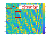
(a)

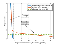
(b)

Figure 3: (a) The heat map of the received pilot signals of the near-field HMIMO channel when the received SNR is 0 dB. The other parameters are set the same as Fig. 2(a). (b) Eigenvalues of the covariance matrices of the virtual subarray channels $\{\mathbf{h}_{t}\in\mathbb{R}^{2d\times 1}\}_{t=1}^{s}$ and the pilots $\{\mathbf{y}_{t}\in\mathbb{R}^{2d\times 1}\}_{t=1}^{s}$, in which the principal and redundant dimensions are separated by a dotted line.

IV Practical Algorithms of the Score-Based Channel Estimator

In this section, we present and analyze practical algorithms for the proposed score-based channel estimator. We first focus on the fully-digital systems in Section IV-A, and then discuss how to extend it to hybrid analog-digital transceivers based on iterative message passing algorithms in Section IV-B. Lastly, we analyze the computational complexity.

IV-A Score-Based Estimator in Fully-Digital Systems

The procedure of the score-based estimator in fully-digital near-field HMIMO systems is summarized in Algorithm 3. In the offline stage, the BS first collects a dataset of received pilot signals $\mathbf{y}$ to train the DAE neural network $\bm{\theta}$ by Algorithm 1. This will cost no additional overhead for the spectral resources, and also does not require knowledge of the noise level. At the online inference stage, Algorithm 3 requires the received pilot signals $\mathbf{y}$, the well-trained DAE parameters $\bm{\theta}$, and the shape of the sliding window for estimating the noise level $\sigma_{\mathbf{\bar{n}}}$. As an initialization, we first employ the trained DAE network $\bm{\theta}$ to approximate the score function using $\nabla_{\mathbf{y}}\log p(\mathbf{y})\approx S_{\bm{\theta}}(\mathbf{y};0)$. Then, Algorithm 2 is executed to obtain the estimated noise level. Finally, we plug the estimated noise level and the score function into (16) to compute the estimated channel. We shall analyze the complexity in Section IV-C, which is extremely low since no costly matrix inversion is required.

Algorithm 3 Bayes-optimal score-based channel estimator for fully-digital HMIMO systems

1:  Input: Received pilots $\mathbf{y}$, trained DAE parameters $\bm{\theta}$, size of the sliding window $\sqrt{d}\times\sqrt{d}$

2:  Output: Estimated near-field HMIMO channel ${\hat{\mathbf{h}}_{\text{MMSE}}}$

3:  Initialize: $\nabla_{\mathbf{y}}\log p(\cdot)\leftarrow S_{\bm{\theta}}(\cdot;0)$

4:  Utilize Algorithm 2 to estimate the noise level $\hat{\sigma}_{\mathbf{n}}$

5:  Compute the estimated channel $\mathbf{\hat{h}}_{\text{MMSE}}$ by using (16)

6:  return $\mathbf{\hat{h}}_{\text{MMSE}}$

In particular, it is worth noting that the algorithm does not require any kind of the prior knowledge of the channel or the noise statistics. Only the received pilot signals $\mathbf{y}$ are required in both the training and the inference stages. Furthermore, only the DAE network $\bm{\theta}$ is parameterized in this algorithm, whose training is unsupervised. Hence, when the EM environment is dynamic, one can keep undating the parameters $\bm{\theta}$ in an online manner to track the changes so as to adapt to the new channel distribution, which will be discussed later in Section V-F.

IV-B Score-Based Estimator in Hybrid Analog-Digital Systems

In this section, we shift the focus to the more general hybrid analog-digital HMIMO systems. We first introduce the general design principle based on iterative message passing algorithms and explain the practical difficulties in applying such methods. Then, we discuss how the score-based estimator and the PCA-based noise level estimation serve as a perfect match to tackle these challenges and enable Bayes-optimal channel estimation for HMIMO in unknown EM environments.

For hybrid analog-digital transceivers, we consider the general system model (9) for CS-based channel estimation. Under such circumstances, Bayes-optimal estimation can be achieved by orthogonal AMP (OAMP) [41, 42], an iterative algorithm with the following update rules consisting of a linear estimator (LE) and a non-linear estimator (NLE), i.e.,

$$\begin{array}[]{cc}&\text{OAMP-LE: }\end{array} \begin{array}[]{cc}\mathbf{r}^{(t)}=\mathbf{h}^{(t)}+\mathbf{W}^{(t)}(\mathbf{y}-\mathbf{M}\mathbf{h}^{(t)}),\end{array}$$ (21)

$$\begin{array}[]{cc}&\text{OAMP-NLE: }\end{array} \begin{array}[]{cc}\mathbf{h}^{(t+1)}=\eta_{t}(\mathbf{r}^{(t)}),\end{array}$$

where the LE is constructed to be de-correlated and the NLE is designed to be a divergence-free function [41]. We say that the LE is de-correlated when $\text{tr}(\mathbf{I}-\mathbf{W}^{(t)}\mathbf{M})=0$ holds, while the divergence-free function can be constructed from an arbitrary function after subtracting its divergence [41]. When both the LE and the NLE are locally MMSE optimal, the replica Bayes-optimality of the OAMP algorithm was conjectured in [41] and rigorously proved in [43]. The term ‘orthogonal’ in the name of OAMP derives from the fact that when the conditions of the LE and the NLE are satisfied, the error after the LE, i.e., $\mathbf{e}^{(t)}\triangleq\mathbf{r}^{(t)}-\mathbf{h}$, consists of independent and identically distributed (i.i.d.) zero-mean Gaussian elements independent of $\mathbf{h}$, and at the same time, the error after the NLE, i.e., $\mathbf{q}^{(t+1)}\triangleq\mathbf{h}^{(t+1)}-\mathbf{h}$, consists of i.i.d. entries independent of $\mathbf{M}$ and $\mathbf{n}$ [41]. Hence, we have that in the $t$-th iteration,

$$\mathbf{r}^{(t)}=\mathbf{h}+\mathbf{e}^{(t)},$$ (22)

in which $\mathbf{h}$ is the ground-truth HMIMO channel, and $\mathbf{e}^{(t)}\sim\mathcal{N}(\mathbf{0},\sigma_{\mathbf{e}^{(t)}}^{2}\mathbf{I})$ is the effective i.i.d. Gaussian noise vector with $\sigma_{\mathbf{e}^{(t)}}$ denoting the noise level. Hence, the NLE should be the Bayes-optimal MMSE denoiser to estimate $\mathbf{h}$ from $\mathbf{r}^{(t)}$, which is essentially the same as the score-based estimator for fully-digital systems proposed in Section IV-A. In addition, the LE should be the linear MMSE (LMMSE) estimator with $\mathbf{W}^{(t)}$ being the LMMSE matrix given by

$$\mathbf{W}^{(t)} =\frac{2N}{\text{tr}(\hat{\mathbf{W}}^{(t)}\mathbf{M})}\mathbf{\hat{W}}^{(t)},\text{\,\,where}$$ (23)

$$\mathbf{\hat{W}}^{(t)} =\sigma_{\mathbf{e}^{(t)}}^{2}\mathbf{M}^{T}(\sigma_{\mathbf{e}^{(t)}}^{2}\mathbf{M}\mathbf{M}^{T}+\sigma_{\mathbf{n}}^{2}\mathbf{I})^{-1}.$$

The coefficient $\frac{2N}{\text{tr}(\hat{\mathbf{W}}^{(t)}\mathbf{M})}$ is multiplied to ensure that the LE is de-correlated. The final estimated channel after $t$ iterations is $\mathbf{h}^{(t+1)}$, which, when converged, is the Bayes-optimal solution.

IV-B1 Challenges of OAMP

Although sounds promising, there are a number of challenges that have hindered the application of OAMP to near-field HMIMO channel estimation.

First, the complexity incurred by the LE is prohibitive when the dimension of the channel $\mathbf{h}\in\mathbb{R}^{2N\times 1}$ becomes extremely large in near-field HMIMO systems, as it requires inverting a $2N\times 2N$ general matrix in each iteration, causing a complexity at the order of $\mathcal{O}(N^{3})$. This is exceedingly large. Second, the noise statistics is unknown. The level $\sigma_{\mathbf{n}}$ of the Gaussian noise $\mathbf{n}$ in the EM environment should be accurately estimated in the first place. Otherwise, both the LE and the NLE cannot be effectively computed. Third, the optimal MMSE estimator in the NLE cannot be constructed without knowledge of the prior distribution of the HMIMO channel $\mathbf{h}$, which, however, is generally not available in practice given the complicated distribution of the near-field HMIMO channel. One should circumvent the prior distribution by other techniques so as to implement the MMSE estimator. In the following, we discuss the practical design of the LE and the NLE to tackle these challenges mainly on the basis of the proposed techniques.

Algorithm 4 Bayes-optimal score-based channel estimator for hybrid analog-digital HMIMO systems

1:  Input: Measurement matrix $\mathbf{M}$, received pilot signals $\mathbf{y}$, trained DAE parameters $\bm{\theta}$, floor value $\xi$, size of the sliding window $\sqrt{d}\times\sqrt{d}$, error tolerance $\epsilon$, maximum allowed number of iterations $T$

2:  Output: Estimated near-field HMIMO channel ${\hat{\mathbf{h}}_{\text{MMSE}}}$

3:  Initialize: $\mathbf{h}^{(0)}\leftarrow\mathbf{0},\mathbf{h}^{(1)}\leftarrow\mathbf{M}^{\dagger}\mathbf{y},t\leftarrow 0,\nabla_{\mathbf{y}}\log p(\cdot)\leftarrow S_{\bm{\theta}}(\cdot;0)$

4:  Obtain $\hat{\sigma}_{\mathbf{n}}$ by Algorithm 2

5:  while $\|\mathbf{h}^{(t+1)}-\mathbf{h}^{(t)}\|>\epsilon$ do

6:      /*OAMP-LE*/     Obtain $\mathbf{r}^{(t)}$ by (21), (23) and (24)     Obtain $\hat{\sigma}_{\mathbf{e}^{(t)}}$ by (25)

7:      /*OAMP-NLE*/     Obtain $\mathbf{h}^{(t+1)}$ by (26)

8:      $t\leftarrow t+1$

9:  ${\hat{\mathbf{h}}_{\text{MMSE}}}\leftarrow\mathbf{h}^{(t+1)}$

10:  return ${\hat{\mathbf{h}}_{\text{MMSE}}}$

IV-B2 Designing the LE

The LMMSE matrix in the LE, i.e., (23), requires the computation of a general matrix inverse with prohibitive complexity. For a general measurement matrix $\mathbf{M}$, the matrix inverse is essential but could be greatly simplified by using the singular value decomposition (SVD) of $\mathbf{M}$, i.e., $\mathbf{\mathbf{M=\mathbf{V}\mathbf{D}}\mathbf{U}^{T}}$, where both $\mathbf{V}$ and $\mathbf{U}$ are orthogonal matrices, and $\mathbf{D}$ is a diagonal matrix. Plugging the SVD of $\mathbf{M}$ into (23), we can get the following results after some algebra, i.e.,

$$\text{$\mathbf{\hat{W}}^{(t)}$} =\sigma_{\mathbf{e}^{(t)}}^{2}\mathbf{M}^{T}(v_{t}^{2}\mathbf{M}\mathbf{M}^{T}+\sigma_{\mathbf{n}}^{2}\mathbf{I})^{-1}$$ (24)

$$=\sigma_{\mathbf{e}^{(t)}}^{2}\mathbf{U}\mathbf{D}^{T}\mathbf{V}^{T}(\sigma_{\mathbf{e}^{(t)}}^{2}\mathbf{\mathbf{V}\mathbf{D}}\mathbf{D}^{T}\mathbf{V}^{T}+\sigma_{\mathbf{n}}^{2}\mathbf{V}\mathbf{I}\mathbf{V}^{T})^{-1}$$

$$=\sigma_{\mathbf{e}^{(t)}}^{2}\mathbf{U}\mathbf{D}^{T}\mathbf{V}^{T}\mathbf{V}(\sigma_{\mathbf{e}^{(t)}}^{2}\mathbf{D}\mathbf{D}^{T}+\sigma_{\mathbf{n}}^{2}\mathbf{I})^{-1}\mathbf{V}^{T}$$

$$=\sigma_{\mathbf{e}^{(t)}}^{2}\mathbf{M}^{T}\mathbf{V}(\sigma_{\mathbf{e}^{(t)}}^{2}\mathbf{D}\mathbf{D}^{T}+\sigma_{\mathbf{n}}^{2}\mathbf{I})^{-1}\mathbf{V}^{T}.$$

Thanks to the SVD operation, we no longer need to calculate a general matrix inverse like (23) in every iteration $t$. Instead, the new expression requires computing the SVD of matrix $\mathbf{M}$ only once, and the computation of (24) becomes much simpler, since $(\sigma_{\mathbf{e}^{(t)}}^{2}\mathbf{D}\mathbf{D}^{T}+\sigma_{\mathbf{n}}^{2}\mathbf{I})$ is diagonal. The complexity of the inverse is cut down drastically from $\mathcal{O}(N^{3})$ to $\mathcal{O}(N)$.

Having solved the complexity issue, another problem is that both the environmental Gaussian noise level of $\mathbf{n}$, i.e., $\sigma_{\mathbf{n}}$, and the effective Gaussian noise level of $\mathbf{e}^{(t)}$, i.e., $\sigma_{\mathbf{e}^{(t)}}$, are both unknown in practice, but should be frequently used in OAMP. For $\hat{\sigma}_{\mathbf{n}}$, it can be estimated from $\mathbf{y}=\text{$\mathbf{Mh}$}+\mathbf{n}$ after treating $\mathbf{Mh}$ as a whole, by using the PCA-based estimator proposed in Algorithm 2. For $\hat{\sigma}_{\mathbf{e}^{(t)}}$, we propose two possible methods to estimate it. First, since $\mathbf{r}^{(t)}=\mathbf{h}+\mathbf{e}^{(t)}$ is similar to the fully-digital system model, i.e., (10), we could apply the PCA-based noise level estimator to $\mathbf{r}^{(t)}$ to get an estimate of $\hat{\sigma}_{\mathbf{e}^{(t)}}$ in each iteration. However, this method requires running Algorithm 2 once per iteration, and incurs a high computational complexity. The second possible option is to utilize the following estimator proposed in [44] for $\hat{\sigma}_{\mathbf{e}^{(t)}}$, given by

$$\hat{\sigma}_{\mathbf{e}^{(t)}}^{2}=\text{max}\{\frac{\|\mathbf{y}-\mathbf{M}\mathbf{h}^{(t)}\|^{2}-2KN_{\text{RF}}\hat{\sigma}_{\mathbf{n}}^{2}}{\text{tr}(\mathbf{M}^{T}\mathbf{M})},\xi\},$$ (25)

where the function $\text{max}\{\cdot\}$ returns the maximum value of the inputs, and $\xi>0$ is set as a small positive value to circumvent numerical instability. The complexity of this approach is much smaller than the first one since it only involves a simple matrix product, and the denominator $\text{tr}(\mathbf{M}^{T}\mathbf{M})$ can be pre-computed. Empirically, we observe that these two methods offer a similar performance. Hence, we pick the latter due to its relative lower computational complexity.

IV-B3 Designing the NLE

Based on (22), $\mathbf{r}^{(t)}$ in each iteration is the ground-truth channel corrupted by white Gaussian noise $\mathbf{e}^{(t)}\sim\mathcal{N}(\mathbf{0},\sigma_{\mathbf{e}^{(t)}}^{2}\mathbf{I})$, which is similar to the formulation in fully-digital systems, i.e., (10). After treating $\mathbf{r}^{(t)}$ as $\mathbf{y}$ and $\hat{\sigma}_{\mathbf{e}^{(t)}}$ as $\hat{\sigma}_{\mathbf{n}}$ in Algorithm 2, the NLE is the same as the score-based estimator in IV-A, given by

$$\mathbf{h}^{(t+1)}=\eta_{t}(\mathbf{r}^{(t)}) \triangleq\mathbf{r}^{(t)}+\hat{\sigma}_{\mathbf{e}^{(t)}}^{2}\nabla_{\mathbf{r}^{(t)}}\log p(\mathbf{r}^{(t)})$$ (26)

$$\approx\mathbf{r}^{(t)}+\hat{\sigma}_{\mathbf{e}^{(t)}}^{2}S_{\bm{\theta}}(\mathbf{r}^{(t)};0).$$

As the effective noise level $\sigma_{\mathbf{e}^{(t)}}$ varies in different numbers of iterations, we pretrain and store a few sets of DAE parameters corresponding to different noise levels and then load different DAE parameters $\bm{\theta}$ according to the estimated noise level $\hat{\sigma}_{\mathbf{e}^{(t)}}$. The complete algorithm for the score-based estimator in hybrid analog-digital systems is summarized in Algorithm 4.

IV-C Complexity Analysis

We first discuss the complexity expressions in fully-digital systems and then extend them to hybrid analog-digital systems.

For fully-digital HMIMO systems, the inference complexity of the proposed score-based algorithm consists of two parts: the computation of the score function $S_{\bm{\theta}}(\mathbf{y};0)$ and the PCA-based estimation of the noise level $\sigma_{\mathbf{n}}$. The former depends on the specific neural architecture of $S_{\bm{\theta}}(\cdot,\cdot)$, and costs a constant complexity, denoted by $p$, once the network is trained. For the latter, we analyze the complexity of Algorithm 2 line by line. The complexity of the virtual subarray decomposition in line 4 is represented as $\mathcal{O}(sd)$. The computation of the mean and covariance in lines 5 and 6 incurs costs of $\mathcal{O}(sd)$ and $\mathcal{O}(sd^{2})$, respectively. The eigenvalue decomposition in line 7 has a complexity of $\mathcal{O}(d^{3})$, while sorting the eigenvalues requires $\mathcal{O}(d^{2})$. The eigenvalue splitting and the noise level estimation, from lines 8 to 14, have a complexity of $\mathcal{O}(d^{2})$. Considering that in HMIMO systems, the approximation $s\thickapprox N$ holds, the complexity of calculating the variance term is approximately $\mathcal{O}(Nd^{2}+d^{3})$. Therefore, the overall complexity for the score-based estimator in fully-digital HMIMO systems, i.e., Algorithm 3, is roughly $\mathcal{O}(Nd^{2}+d^{3}+p)$, which scales linearly with the number of antennas $N$. In practice, the fluctuation of the received SNR may not be frequent. In such a case, it is not a necessity to estimate the received SNR for every instance of the received pilot signals $\mathbf{y}$. Therefore, the actual complexity of the proposed score-based algorithm is within the range of $\mathcal{O}(p)$ and $\text{$\mathcal{O}$}(Nd^{2}+d^{3}+p)$, which is extremely efficient given the near-optimal performance.

For hybrid analog-digital HMIMO systems, we analyze the per-iteration complexity of Algorithm 4. We first analyze the LE. Thanks to the SVD-based method, we no longer need to compute a costly general matrix inversion in each iteration. If the SVD of matrix $\mathbf{M}$ is pre-computed and cached, only the inversion of a diagonal matrix is required per iteration, which only incurs a complexity of $\mathcal{O}(N)$. Hence, the complexity of the LE is only dominated by the matrix-vector product with complexity $\mathcal{O}(NKN_{\text{RF}})$. The overall complexity of the LE is $\mathcal{O}(NKN_{\text{RF}}+N)$. For the NLE, the complexity involves one forward propagation of the neural network $\bm{\theta}$, which is of a constant complexity $p$. Therefore, the per-iteration complexity of the score-based estimator in hybrid analog-digital systems is $\mathcal{O}(NKN_{\text{RF}}+N+p)$, dominated by the matrix-vector product. In addition, before the iterations, we need to run the PCA-based Algorithm 2 only once to estimate the Gaussian noise level in the environment, which costs $\mathcal{O}(Nd^{2}+d^{3})$.

V Simulation Results

V-A Simulation Setup

We consider uplink channel estimation in a typical HMIMO system whose general parameters are listed in Table I. Specifically, the antenna spacings are configured to be smaller than the nominal value of half the carrier wavelength $\lambda_{c}$ to model the quasi-continuous aperture in HMIMO systems. In addition, the distance between the BS and the scatterer ring is set within the near-field region, i.e., $S\ll d_{\text{Rayleigh}}$.

The following baselines are compared in the simulations.

TABLE I: General parameters of the HMIMO system

Parameter	Value
Number of antennas	$N=1024$
Carrier frequency	$f_{c}=16$ GHz
Carrier wavelength	$\lambda_{c}=1.88\times 10^{-2}$ m
Antenna spacing	$d_{a}=\frac{\lambda_{c}}{6}=3.12\times 10^{-3}$ m
Rayleigh distance	$d_{\text{Rayleigh}}=1.09\times 10^{3}$ m
Distance of the scatterer ring	$S=10$ m
Radius of the scatterer ring	$R=3$ m
Direction of the scatterer ring	$\Psi=\frac{\pi}{3}$ rad
Mean of the scatterer angle	$\mu=\frac{\pi}{4}$ rad
Concentration of the scatterer angle	$\kappa=0$ rad

TABLE II: Performance of the noise level estimation

$\sigma_{\mathbf{\mathbf{\bar{n}}}}$ / (SNR)	Method	Bias	Std	RMSE	Percent error
0.5623 (5 dB)	Oracle	0.0002	0.0087	0.0087	1.55%
	Proposed	0.0044	0.0153	0.0159	2.83%
	Sparsity	0.0344	0.0142	0.0372	6.62%
0.1778 (15 dB)	Oracle	<0.0001	0.0027	0.0027	1.52%
	Proposed	0.0029	0.0043	0.0052	2.92%
	Sparsity	0.0209	0.0087	0.0227	12.77%
0.0562 (25 dB)	Oracle	<0.0001	0.0009	0.0009	1.60%
	Proposed	0.0004	0.0013	0.0014	2.49%
	Sparsity	0.0208	0.0125	0.0243	43.24%

• LS: Least squares estimation.

  

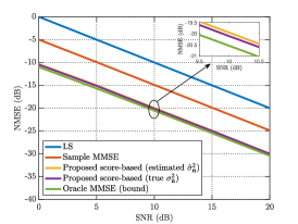
  (a)

  

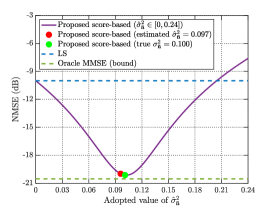
  (b)

  

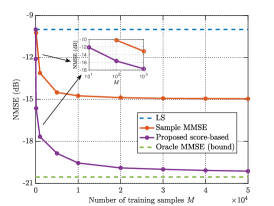
  (c)

  Figure 4: Simulation results in fully-digital systems. (a) NMSE as a function of the received SNR in fully-digital transceivers. (b) The influence of the accuracy of the received SNR estimation on the NMSE performance, when the received SNR is 10 dB. (c) Sample complexity of the proposed score-based estimator, where the NMSE is illustrated as a function of the number of training samples $M$. The received SNR when plotting this figure is 10 dB.

• Oracle MMSE: Oracle MMSE is the MMSE estimator that has a perfect knowledge of both the spatial correlation matrix $\mathbf{R}_{\text{NF}}$ and the noise level $\sigma_{\bar{\mathbf{n}}}$, given by

  $$\mathbf{\hat{h}}_{\text{oracle-MMSE}}=\mathbf{R}_{\text{NF}}\text{$\mathbf{M}$}^{H}(\mathbf{M}\mathbf{R}_{\text{NF}}\mathbf{M}^{H}+\sigma_{\mathbf{\bar{n}}}^{2}\mathbf{I})^{-1}\bar{\mathbf{y}}.$$ (27)

  Note that since the HMIMO channel follows a correlated Rayleigh fading, the linear MMSE is the optimal MMSE estimator that provides the Bayesian performance bound. It is also worth noting that $\mathbf{R}_{\text{RF}}$ is extremely difficult, if not impossible, to be acquired in practice since it contains $N^{2}$ entries and is thus prohibitive to estimate when $N$ is particularly large in HMIMO systems.

• Sample MMSE: Sample MMSE estimator has the same expression as (27), but replaces the true spatial correlation $\mathbf{R}_{\text{NF}}$ with an estimated one $\mathbf{R}_{\text{sample}}$ based upon the testing samples, given by $\mathbf{R}_{\text{sample}}\triangleq\frac{1}{L}\sum_{l=1}^{L}\mathbf{y}_{l}\mathbf{y}_{l}^{H}-\sigma_{\mathbf{\bar{n}}}^{2}\mathbf{I}$ [27], in which $L$ is the number of testing samples and $\mathbf{y}_{l}$ is the $l$-th sample of the received pilots in the testing dataset. We also utilize the perfect noise level $\sigma_{\mathbf{\bar{n}}}$ in sample MMSE.

During the training stage, the hyper-parameters in the proposed score-based estimator are selected as $\gamma=0.0004$, $\sigma^{\text{min}}=0.001$, $\sigma^{\text{max}}=0.1$, $Q=100$, and $M=50\text{,}000$. In addition, we adopt a batch size of 16 and reduce the learning rate $\gamma$ by half after every 25 epochs. In the inference stage, the shape of the sliding window in the PCA-based noise level estimation algorithm is $5\times 5$. The performance is evaluated based on the normalized MSE (NMSE) on a testing dataset with $L=10,000$ samples, i.e., $\text{NMSE}\triangleq\text{$\mathbb{E}$}\nicefrac{{\|\mathbf{h}-\mathbf{\hat{h}}\|^{2}}}{{\|\mathbf{h}\|^{2}}}$. For the neural architecture of the DAE $S_{\bm{\theta}}(\cdot;\cdot)$, we adopt a simplified UNet architecture [45]. Note that depending on the complexity budget, many other prevailing neural architectures could also be applied [13].

In the following, we first evaluate the accuracy of the PCA-based noise level estimation, which is a crucial component of the proposed score-based estimator. Subsequently, we provide extensive simulations for the score-based estimator in both the fully-digital and the hybrid analog-digital HMIMO systems, in terms of estimation accuracy, sample complexity, robustness, and online adaptation capability.

V-B Accuracy of the PCA-Based Noise Level Estimation

The accuracy of the noise level estimation has an impact on the NMSE performance of the proposed score-based estimator. Hence, different from most previous works that have assumed a perfect knowledge of the noise level $\sigma_{\bar{\mathbf{n}}}$, we alleviate such an assumption and propose a PCA-based method to estimate it. In Table II, we list the estimation accuracy under different SNRs, where $\hat{\sigma}_{\mathbf{\bar{n}}}$ denotes the estimated noise level. The bias, the standard deviation (std), and the root MSE (RMSE) of the estimator are given by $\mathbb{E}[|\sigma_{\mathbf{\bar{n}}}-\mathbb{E}[\hat{\sigma}_{\mathbf{\bar{n}}}]|]$, $\sqrt{\mathbb{E}[(\hat{\sigma}_{\mathbf{\bar{n}}}-\mathbb{E}[\hat{\sigma}_{\mathbf{\bar{n}}}])^{2}]}$, and $\sqrt{\mathbb{E}[(\sigma_{\bar{\mathbf{n}}}-\hat{\sigma}_{\mathbf{\bar{n}}})^{2}]}$, respectively. The RMSE gives an overall assessment of the performance, while the bias and the std reflect the accuracy and robustness of different estimators. We also provide the percent error, defined as $\nicefrac{{\text{RMSE}}}{{\sigma_{\mathbf{\bar{n}}}}}$, to show the error as a percentage of the true noise level. We compare the proposed PCA-based method with the following benchmarks.

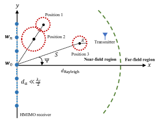
(a)

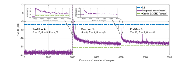
(b)

Figure 5: Online adaptation in dynamic environments. (a) The positions of the scatterer rings with different values of direction $\Psi$, radius $R$, and distance $S$. (b) NMSE versus the number of pilot transmission slots during the online adaptation process, when the received SNR is 10 dB.

• Sparsity-based: The squared median absolute deviation (MAD) algorithm for the noise level estimation of sparse signals [46]. Similar to [46], we utilize the estimator after transforming the channel into the angular domain.

• Oracle bound: Assume perfect knowledge of the ground-truth channel $\bar{\mathbf{h}}$, and estimate the noise level directly from $\mathbf{\bar{n}}=\mathbf{\bar{y}}-\mathbf{\bar{h}}$ by using sample standard deviation, which is the minimum variance unbiased estimator.

Since the sparsity-based algorithm was originally proposed for the complex-valued case, we perform the comparison using the complex-valued version of the proposed PCA-based method, which offers a similar performance as the real-valued version.

Table II compares the performance of different noise level estimators. As shown in the table, the proposed method has a comparable RMSE with the oracle bound and significantly outperforms the sparsity-based algorithm. The advantages of our proposal are consistent across different SNR levels, with a negligible percent error of less than 3%. This indicates that the proposed method can effectively exploit the low-rank property of the near-field spatial correlation. By contrast, the sparsity-based algorithm performs poorly since the near-field HMIMO channel lacks sparsity in the angular domain. Later, in Section V-D, we will illustrate that the proposed score-based channel estimator is robust to SNR estimation errors, and the accuracy of the PCA-based estimator will cause almost no performance loss compared to using the true noise level.

V-C Estimation Accuracy in Fully-Digital Systems

In Fig. 4(a), we plot the NMSE performance as a function of the received SNR $\rho$ in fully-digital HMIMO transceivers, in which $N_{\text{RF}}=N$. We depict two lines for the proposed score-based estimator. The yellow one refers to the performance when the PCA-estimated noise level is adopted in (16), while the purple line corresponds to the case in which the perfect noise level is utilized. It is observed that these two lines largely overlap, indicating that the PCA-estimated noise level provides almost the same performance as the perfect noise level. Additionally, the proposed score-based algorithm significantly outperforms the LS and the sample MMSE estimators by over 10 dB and 5 dB, respectively, in terms of NMSE, and achieves arguably the same NMSE performance (with a negligible 0.6 dB drop) as the oracle MMSE performance bound. The competitive results are consistent in different SNR ranges. Notice that the oracle MMSE method utilizes the true covariance and noise level, but the proposed method requires neither. This demonstrates the strong capability of the unsupervised score-based estimator to achieve a near-Bayes-optimal performance without any oracle information in unknown EM environments.

V-D Robustness to Noise Level Estimation Errors

In Fig. 4(b), we illustrate the how the accuracy of the estimated noise level will affect the performance of the proposed score-based estimator. In the simulations, the true noise level is set as $\sigma_{\mathbf{\bar{n}}}=0.1$, corresponding to an SNR of 10 dB. We vary the adopted values of $\hat{\sigma}_{\mathbf{\bar{n}}}$ in (16) within $\hat{\sigma}_{\mathbf{\bar{n}}}\in[0,0.24]$, and plot the corresponding NMSE performance curve in blue. Particularly, we utilize red and green dots to denote the NMSE achieved with the estimated and true SNR values, respectively. The LS and the oracle MMSE algorithms are presented as the performance upper and lower bounds. It is observed that even when an inexact received SNR is adopted, the performance of the score-based algorithm is still quite robust and significantly outperforms the LS method. Also, the estimated received SNR by the PCA-based method is accurate enough to offer a near-optimal performance, even in unknown EM environments.

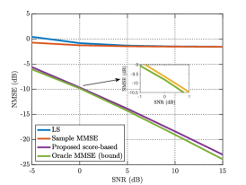
(a)

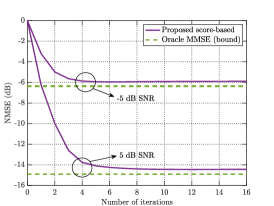
(b)

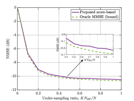
(c)

Figure 6: Simulation results in hybrid analog-digital systems. (a) NMSE versus the received SNR when the under-sampling ratio is $KN_{\text{RF}}/N=0.3$. (b) NMSE as a function of the iteration number when the under-sampling ratio is $KN_{\text{RF}}/N=0.5$. (c) NMSE as a function of different under-sampling ratio $KN_{\text{RF}}/N$ when the received SNR is set as 0 dB.

V-E Sample Complexity

In Fig. 4(c), we study the sample complexity of the proposed score-based estimator, where the NMSE is shown as a function of the number of training samples $M$. The received SNR when plotting the figure is 10 dB. We notice that the gap between the proposed score-based estimator and the oracle MMSE bound gradually vanishes when $M$ increases. The NMSE gap shrinks to less than 1 dB at $M=10,000$, and further reduces to less than 0.5 dB when $M=30,000$. The sample complexity curve of the proposed estimator follows a similar trend as the sample MMSE method, whose performance both starts to saturate as $M$ reaches 10,000. Additionally, we are also interested in the low-sample region when fewer than 1,000 training samples are available. The region is zoomed in and shown in the subfigure. It is observed that, the score-based estimator can bring a 2 dB margin with only $M=10$ training samples, and further bring a 6 dB advantage with $M=100$ samples, as compared to the LS estimator. This confirms that the effectiveness of the proposal in different sample regions. As a final comment, we emphasize again that the training process is totally unsupervised and only the received pilot signals $\mathbf{y}$ are required.

V-F Online Adaptation in Dynamic Environments

Since the proposed score-based method is unsupervised, and only requires the received pilot signals $\mathbf{y}$ during training, it is possible to update the network parameters $\bm{\theta}$ in an online manner to adapt to the dynamic EM environments. To illustrate the idea, we consider a dynamic environment as shown in Fig. 5(a), which labels three possible positions of the scatterers. We assume that the scatterers gradually move from positions 1 to 3 to model the dynamic EM environment, and that each position lasts for 2,000 pilot transmission slots.

We keep running Algorithm 1 so as to update the parameters of the network parameters $\bm{\theta}$ of the score function. Since the received pilot signals $\mathbf{y}$ arrive one by one in an online manner, we utilize a batch size of 1 and update the network parameters once a new sample is received. In addition, we also change the hyper-parameters to $\gamma=0.0006$, $\varsigma^{\text{min}}=0.001$, $\varsigma^{\text{max}}=0.1$, and keep the learning rate $\gamma$ constant.

In Fig. 5(a), we illustrate the 3 positions of the scatterer ring with different values of direction $\Psi$, radius $R$, and distance $S$, which are labeled in Fig. 5(b). We depict the online adaptation performance as a function of the number of pilot transmission slots. We assume that the parameters of the network, i.e., $\bm{\theta}$, are well trained offline for position 1 as described in Section V-A. By contrast, the scatterer rings in positions 2 and 3 are never seen before in the offline training stage, but suddenly appear in online deployment. For clarity, we zoom in the transition phase between different scatterer positions.

From the results in position 1, it is observed that the online adaptation will not have negative influence on the performance of the well-trained network parameters $\bm{\theta}$. During the transition phase from positions 1 to 2, we first observe an abrupt increase in NMSE. However, after a few pilot transmission slots, the online adaptation algorithm quickly recovers the performance to a remarkable level that is close to the oracle MMSE bound. The performance improves steadily with more samples. A quite similar curve also appears during the transition from positions 2 to 3. These results confirm the effectiveness of the proposed score-based estimator in handling the uncertainties in the EM environments, which is crucial in practical deployment. The running time complexity of the online adaptation process is less than 0.01 s per sample on a Nvidia A40 GPU. This ensures a real-time adaptation to dynamic environments.

V-G Estimation Accuracy in Hybrid Analog-Digital Systems

In Fig. 6(a), we plot the NMSE as a function of the received SNR when the under-sampling ratio $KN_{\text{RF}}/N$ equals 0.3 in hybrid analog-digital HMIMO transceivers. We find that under such a low under-sampling ratio, the performance gain of the sample MMSE algorithm is marginal as compared to the LS estimator. By contrast, the performance of the proposed score-based method still remains close to the oracle MMSE bound across different SNR levels. As observed, the gap to the oracle bound becomes slighter larger in the high SNR region. Nevertheless, it is still significantly better than other baselines.

In Fig. 6(b), we illustrate the NMSE performance at different number of iterations when the under-sampling ratio $KN_{\text{RF}}/N$ is 0.5 in hybrid analog-digital systems. As observed from the figure, the score-based OAMP algorithm converges rapidly to the oracle bound within only about 5 iterations, which proves its supreme efficiency and validates our convergence analysis. It is also interesting to notice that the NMSE is monotonically decreasing with more iterations. This enables a flexible trade-off between complexity and performance.

In Fig. 6(c), we examine the effectiveness of the score-based OAMP algorithm under different under-sampling ratios when the received SNR is set as 0 dB. The performance trend of the our proposal aligns well with the oracle bound. The gap vis-a-vis the bound is consistently smaller than 0.5 dB even under extremely small under-sampling ratios, e.g., $KN_{\text{RF}}/N=0.1$. This indicates that our proposed method can seamlessly generalize to the different pilot lengths $K$ that may be encountered in practice. It is also interesting to observe that, the NMSE of both curves decreases quickly when the under-sampling ratio increases from 0 to 0.4, and gradually saturates thereafter. This confirms that the pilot overhead for near-field HMIMO channel estimation can be significantly reduced with proper prior information about the channel. The similar NMSE trend to the oracle bound also indicates that the score-based method leads to a near-optimal pilot overhead, and confirms that it effectively learns the prior distribution of the near-field HMIMO channel in a totally unsupervised manner.

VI Conclusions and Future Directions

Leveraging the connection between the MMSE estimator and the score-function, in this paper, we proposed an innovative unsupervised learning framework for channel estimation in near-field HMIMO systems. Different from existing methods, the proposed algorithms are trained solely based on the received pilots, without requiring any kind of prior knowledge of the HMIMO channel or the noise statistics. This enables it to work in arbitrary and unknown EM environments that may appear in real-world deployment. The key components of the proposed framework, i.e., learning the score function, the PCA-based noise level estimation, and the iterative message passing algorithms, are presented along with theoretical underpinnings. Extensive simulation results have demonstrated that our proposal can achieve promising performance in both fully-digital and hybrid analog-digital systems, reaching an NMSE value close to the oracle MMSE bound with significant reduction in complexity. Furthermore, we provided relevant simulation results to validate its strong robustness and the online adaptation to dynamic EM environments without any priors or supervision. The results have clearly proven the effectiveness of the score-based unsupervised learning framework for designing Bayes-optimal channel estimators in near-field HMIMO systems. As future directions, it is interesting to extend our proposal to low-resolution HMIMO transceivers [47] and incorporate advanced meta-learning algorithms to improve the efficiency of the online adaptation process.

Appendix A Proof of Theorem 3

Define the covariance of $\{\mathbf{y}_{t}\in\mathbb{R}^{2d\times 1}\}_{t=1}^{s}$ as

$$\bm{\Sigma}_{\mathbf{y}_{t}}=\frac{1}{s}\sum_{t=1}^{s}(\mathbf{y}_{t}-\bm{\mu})(\mathbf{y}_{t}-\bm{\mu})^{T},$$ (28)

in which $\bm{\mu}\triangleq\frac{1}{s}\sum_{t=1}^{s}\mathbf{y}_{t}$ is the mean vector. The eigenvalue decomposition of $\bm{\Sigma}_{\mathbf{y}_{t}}$ is given by

$$\bm{\Sigma}_{\mathbf{y}_{t}}=\mathbf{R}\bm{\text{$\Lambda$}}\mathbf{R}^{T}=\mathbf{R}\text{\text{diag}($\lambda_{1},\lambda_{2},\ldots,\lambda_{r}$)}\mathbf{R}^{T},\,\,\text{where\,\,}r=4d^{2}.$$ (29)

We can represent $\mathbf{y}_{t}$ by using the eigenvector matrix $\mathbf{R}$ as a basis, i.e., $\mathbf{y}_{t}=\mathbf{R}\bm{\beta}_{t}$, with $\mathbf{R}\mathbf{R}^{T}=\mathbf{I}$. Assuming that $\mathbf{h}_{t}$ lies in a $m$-dim subspace ($m\ll r$) and could be represented as $\mathbf{h}_{t}=\mathbf{A}\bm{\alpha}_{t}$, where $\mathbf{R}=[\mathbf{A},\mathbf{U}]$ with $\mathbf{A}\in\mathbb{R}^{r\times m}$ consisting of the $m$ eigenvectors corresponding to the $m$ largest eigenvalues, we have that

$$\mathbf{y}_{t}=\mathbf{R}\bm{\beta}_{t}=[\mathbf{A},\mathbf{U}]\left[\begin{array}[]{c}\bm{\alpha}_{t}\\ \mathbf{0}\end{array}\right]+\mathbf{n}_{t},$$ (30)

Multiplying both sides with $\mathbf{R}^{T}$, we obtain that

$$\mathbf{R}^{T}\mathbf{y}_{t}=\left[\begin{array}[]{c}\bm{\alpha}_{t}\\ \mathbf{0}\end{array}\right]+\text{[}\mathbf{A},\mathbf{U}]^{T}\mathbf{n}_{t}=\left[\begin{array}[]{c}\bm{\alpha}_{t}+\mathbf{A}^{T}\mathbf{n}_{t}\\ \mathbf{U}^{T}\mathbf{n}_{t}\end{array}\right],$$ (31)

in which $\mathbf{U}^{T}\mathbf{n}_{t}$ follows $\mathcal{N}(\mathbf{0},\sigma_{\mathbf{n}}^{2}\mathbf{I})$ according to the property of Gaussian distribution. It is observed that the noise $\mathbf{n}_{t}$ has been separated from the measurement $\mathbf{y}_{t}$ by matrix $\mathbf{R}$. Hence, the covariance of $\mathbf{R}^{T}\mathbf{y}_{t}$ is

$$\frac{1}{s}\sum_{t=1}^{s}(\mathbf{R}^{T}\mathbf{y}_{t})(\mathbf{R}^{T}\mathbf{y}_{t})^{T}=\mathbf{R}^{T}\bm{\Sigma}_{\mathbf{y}_{t}}\mathbf{R}=\bm{\Lambda},$$ (32)

from which we easily conclude that the redundant eigenvalues follow a Gaussian distribution with variance $\sigma_{\mathbf{n}}^{2}$.

References

- [1] W. Yu, H. He, X. Yu, S. Song, J. Zhang, R. D. Murch, and K. B. Letaief, “Learning Bayes-optimal channel estimation for holographic MIMO in unknown EM environments,” arXiv preprint arXiv:2311.07908, 2023.
- [2] A. Pizzo, T. L. Marzetta, and L. Sanguinetti, “Spatially-stationary model for holographic MIMO small-scale fading,” IEEE J. Sel. Areas Commun., vol. 38, no. 9, pp. 1964–1979, Sept. 2020.
- [3] A. Pizzo, L. Sanguinetti, and T. L. Marzetta, “Fourier plane-wave series expansion for holographic MIMO communications,” IEEE Trans. Wireless Commun., vol. 21, no. 9, pp. 6890–6905, Sept. 2022.
- [4] O. T. Demir, E. Bjornson, and L. Sanguinetti, “Channel modeling and channel estimation for holographic massive MIMO with planar arrays,” IEEE Wireless Commun. Lett., vol. 11, no. 5, pp. 997–1001, May 2022.
- [5] L. Wei, C. Huang, G. C. Alexandropoulos, W. E. I. Sha, Z. Zhang, M. Debbah, and C. Yuen, “Multi-user holographic MIMO surfaces: Channel modeling and spectral efficiency analysis,” IEEE J. Sel. Topics Signal Process., vol. 16, no. 5, pp. 1112–1124, Aug. 2022.
- [6] T. Wang, Y. Liu, M. Zhang, W. E. I. Sha, C. Ling, C. Li, and S. Wang, “Channel measurement for holographic MIMO: Benefits and challenges of spatial oversampling,” in IEEE Int. Conf. Commun., Rome, Italy, May-Jun. 2023, pp. 5036–5041.
- [7] R. Deng, B. Di, H. Zhang, Y. Tan, and L. Song, “Reconfigurable holographic surface: Holographic beamforming for metasurface-aided wireless communications,” IEEE Trans. Veh. Technol., vol. 70, no. 6, pp. 6255–6259, Jun. 2021.
- [8] J. An, C. Xu, D. W. K. Ng, G. C. Alexandropoulos, C. Huang, C. Yuen, and L. Hanzo, “Stacked intelligent metasurfaces for efficient holographic MIMO communications in 6G,” IEEE J. Sel. Areas Commun., vol. 41, no. 8, pp. 2380–2396, Aug. 2023.
- [9] L. Wei, C. Huang, G. C. Alexandropoulos, Z. Yang, J. Yang, W. E. I. Sha, Z. Zhang, M. Debbah, and C. Yuen, “Tri-polarized holographic MIMO surfaces for near-field communications: Channel modeling and precoding design,” IEEE Trans. Wireless Commun., pp. 1–1, to appear, 2023.
- [10] A. A. D’Amico, A. d. J. Torres, L. Sanguinetti, and M. Win, “Cramer-Rao bounds for holographic positioning,” IEEE Trans. Signal Process., vol. 70, pp. 5518–5532, Nov. 2022.
- [11] A. Elzanaty, A. Guerra, F. Guidi, D. Dardari, and M.-S. Alouini, “Toward 6G holographic localization: Enabling technologies and perspectives,” IEEE Internet Things Mag., vol. 6, no. 3, pp. 138–143, Sept. 2023.
- [12] H. Zhang, H. Zhang, B. Di, M. D. Renzo, Z. Han, H. V. Poor, and L. Song, “Holographic integrated sensing and communication,” IEEE J. Sel. Areas Commun., vol. 40, no. 7, pp. 2114–2130, Jul. 2022.
- [13] W. Yu, Y. Ma, H. He, S. Song, J. Zhang, and K. B. Letaief, “AI-native transceiver design for near-field ultra-massive MIMO: Principles and techniques,” arXiv preprint arXiv:2309.09575, 2023.
- [14] M. Cui and L. Dai, “Channel estimation for extremely large-scale MIMO: Far-field or near-field?” IEEE Trans. Commun., vol. 70, no. 4, pp. 2663–2677, Apr. 2022.
- [15] Y. Liu, Z. Tan, H. Hu, L. J. Cimini, and G. Y. Li, “Channel estimation for OFDM,” IEEE Commun. Surv. Tut., vol. 16, no. 4, pp. 1891–1908, Fourthquarter, 2014.
- [16] S. Liu, X. Yu, Z. Gao, and D. W. K. Ng, “DPSS-based codebook design for near-field XL-MIMO channel estimation,” arXiv preprint arXiv:2310.18180, 2023.
- [17] H. Xie, F. Gao, and S. Jin, “An overview of low-rank channel estimation for massive MIMO systems,” IEEE Access, vol. 4, pp. 7313–7321, Nov. 2016.
- [18] Y. Zhu, H. Guo, and V. K. N. Lau, “Bayesian channel estimation in multi-user massive MIMO with extremely large antenna array,” IEEE Trans. Signal Process., vol. 69, pp. 5463–5478, Sept. 2021.
- [19] W. Yu, Y. Shen, H. He, X. Yu, S. Song, J. Zhang, and K. B. Letaief, “An adaptive and robust deep learning framework for THz ultra-massive MIMO channel estimation,” IEEE J. Sel. Topics Signal Process., vol. 17, no. 4, pp. 761–776, Jul. 2023.
- [20] H. He, S. Jin, C.-K. Wen, F. Gao, G. Y. Li, and Z. Xu, “Model-driven deep learning for physical layer communications,” IEEE Wireless Commun., vol. 26, no. 5, pp. 77–83, Oct. 2019.
- [21] E. Balevi, A. Doshi, A. Jalal, A. Dimakis, and J. G. Andrews, “High dimensional channel estimation using deep generative networks,” IEEE J. Sel. Areas Commun., vol. 39, no. 1, pp. 18–30, Jan. 2021.
- [22] X. Zheng and V. K. N. Lau, “Online deep neural networks for mmwave massive MIMO channel estimation with arbitrary array geometry,” IEEE Trans. Signal Process., vol. 69, pp. 2010–2025, Mar. 2021.
- [23] H. He, R. Wang, W. Jin, S. Jin, C.-K. Wen, and G. Y. Li, “Beamspace channel estimation for wideband millimeter-wave MIMO: A model-driven unsupervised learning approach,” IEEE Trans. Wireless Commun., vol. 22, no. 3, pp. 1808–1822, Mar. 2023.
- [24] W. Yu, H. He, X. Yu, S. Song, J. Zhang, and K. B. Letaief, “Blind performance prediction for deep learning based ultra-massive MIMO channel estimation,” in Proc. IEEE Int. Conf. Commun., Rome, Italy, May-Jun. 2023.
- [25] J. An, C. Yuen, C. Huang, M. Debbah, H. V. Poor, and L. Hanzo, “A tutorial on holographic MIMO communications–part I: Channel modeling and channel estimation,” IEEE Commun. Lett., vol. 27, no. 7, pp. 1664–1668, Jul. 2023.
- [26] H. He, C.-K. Wen, S. Jin, and G. Y. Li, “Model-driven deep learning for MIMO detection,” IEEE Trans. Signal Process., vol. 68, pp. 1702–1715, Feb. 2020.
- [27] A. A. D’Amico, G. Bacci, and L. Sanguinetti, “DFT-based channel estimation for holographic MIMO,” in Proc. Asilomar Conf. Signals Syst. Comput., Pacific Grove, CA, USA, Nov. 2023.
- [28] Z. Wan, Z. Gao, F. Gao, M. D. Renzo, and M.-S. Alouini, “Terahertz massive MIMO with holographic reconfigurable intelligent surfaces,” IEEE Trans. Commun., vol. 69, no. 7, pp. 4732–4750, Jul. 2021.
- [29] E. Bjornson and L. Sanguinetti, “Rayleigh fading modeling and channel hardening for reconfigurable intelligent surfaces,” IEEE Wireless Commun. Lett., vol. 10, no. 4, pp. 830–834, Apr. 2021.
- [30] Z. Dong and Y. Zeng, “Near-field spatial correlation for extremely large-scale array communications,” IEEE Commun. Lett., vol. 26, no. 7, pp. 1534–1538, Jul. 2022.
- [31] A. Abdi, J. Barger, and M. Kaveh, “A parametric model for the distribution of the angle of arrival and the associated correlation function and power spectrum at the mobile station,” IEEE Trans. Veh. Technol., vol. 51, no. 3, pp. 425–434, May 2002.
- [32] A. de Jesus Torres, L. Sanguinetti, and E. Bjornson, “Electromagnetic interference in RIS-aided communications,” IEEE Wireless Commun. Lett., vol. 11, no. 4, pp. 668–672, Apr. 2022.
- [33] J. Zhang, X. Yu, and K. B. Letaief, “Hybrid beamforming for 5G and beyond millimeter-wave systems: A holistic view,” IEEE Open J. Commun. Soc., vol. 1, pp. 77–91, Dec. 2019.
- [34] G. Alain and Y. Bengio, “What regularized auto-encoders learn from the data-generating distribution,” J. Mach. Learn. Res., vol. 15, no. 1, pp. 3563–3593, Nov. 2014.
- [35] Z. Gulgun and E. G. Larsson, “Massive MIMO with Cauchy noise: Channel estimation, achievable rate and data decoding,” IEEE Trans. Wireless Commun., pp. 1–1, to appear, 2023.
- [36] M. Raphan and E. P. Simoncelli, “Least squares estimation without priors or supervision,” Neural Comput., vol. 23, no. 2, pp. 374–420, Feb. 2011.
- [37] K. He, X. Zhang, S. Ren, and J. Sun, “Deep residual learning for image recognition,” in Proc. IEEE Conf. Comput. Vis. Pattern Recog., Las Vegas, NV, USA, Jun. 2016.
- [38] J. H. Lim, A. Courville, C. Pal, and C.-W. Huang, “AR-DAE: towards unbiased neural entropy gradient estimation,” in Proc. Int. Conf. Mach. Learn., Virtual, Jul. 2020.
- [39] H. Lu, Y. Zeng, C. You, Y. Han, J. Zhang, Z. Wang, Z. Dong, S. Jin, C.-X. Wang, T. Jiang, X. You, and R. Zhang, “A tutorial on near-field XL-MIMO communications towards 6G,” arXiv preprint arXiv:2310.11044, 2023.
- [40] S. S. Shapiro and M. B. Wilk, “An analysis of variance test for normality (complete samples),” Biometrika, vol. 52, no. 3/4, pp. 591–611, Dec. 1965.
- [41] J. Ma and L. Ping, “Orthogonal AMP,” IEEE Access, vol. 5, pp. 2020–2033, Jan. 2017.
- [42] Q. Zou and H. Yang, “A concise tutorial on approximate message passing,” arXiv preprint arXiv:2201.07487, 2022.
- [43] K. Takeuchi, “Rigorous dynamics of expectation-propagation-based signal recovery from unitarily invariant measurements,” IEEE Trans. Inf. Theory, vol. 66, no. 1, pp. 368–386, Jan. 2020.
- [44] J. P. Vila and P. Schniter, “Expectation-maximization Gaussian-mixture approximate message passing,” IEEE Trans. Signal Process., vol. 61, no. 19, pp. 4658–4672, Oct. 2013.
- [45] O. Ronneberger, P. Fischer, and T. Brox, “U-net: Convolutional networks for biomedical image segmentation,” in Proc. Int. Conf. Med. Image Comput. Comput.-Assisted Intervention, Munich, Germany, Oct. 2015.
- [46] A. Gallyas-Sanhueza and C. Studer, “Low-complexity blind parameter estimation in wireless systems with noisy sparse signals,” IEEE Trans. Wireless Commun., vol. 22, no. 10, pp. 7055–7071, Oct. 2023.
- [47] H. He, C.-K. Wen, and S. Jin, “Bayesian optimal data detector for hybrid mmwave MIMO-OFDM systems with low-resolution ADCs,” IEEE J. Sel. Topics Signal Process., vol. 12, no. 3, pp. 469–483, Jun. 2018.