Take History as a Mirror in Heterogeneous Federated Learning

Abstract

Federated Learning (FL) allows several clients to cooperatively train machine learning models without disclosing the raw data. In practice, due to the system and statistical heterogeneity among devices, synchronous FL often encounters the straggler effect. In contrast, asynchronous FL can mitigate this problem, making it suitable for scenarios involving numerous participants. However, Non-IID data and stale models present significant challenges to asynchronous FL, as they would diminish the practicality of the global model and even lead to training failures. In this work, we propose a novel asynchronous FL framework called Federated Historical Learning (FedHist), which effectively addresses the challenges posed by both Non-IID data and gradient staleness. FedHist enhances the stability of local gradients by performing weighted fusion with historical global gradients cached on the server. Relying on hindsight, it assigns aggregation weights to each participant in a multi-dimensional manner during each communication round. To further enhance the efficiency and stability of the training process, we introduce an intelligent $\ell_{2}$-norm amplification scheme, which dynamically regulates the learning progress based on the $\ell_{2}$-norms of the submitted gradients. Extensive experiments demonstrate that FedHist outperforms state-of-the-art methods in terms of convergence performance and test accuracy.

Introduction

As a distributed machine learning paradigm, Federated learning (FL) (Konečnỳ et al. 2016; McMahan et al. 2017) has garnered widespread attention in recent years due to its ability to protect the privacy of end-user data. In a classical FL workflow, each client uses its private data to train a local model and then uploads the gradient to a central server. The central server aggregates the collected local gradients into a global gradient to update the global model, which is then sent back to the clients for subsequent training rounds. The entire process does not leak the raw data. As such, FL effectively safeguards data privacy and provides unique advantages in various domains including healthcare (Brisimi et al. 2018), autonomous driving (Liang et al. 2022), and mobile keyboard prediction (Hard et al. 2018).

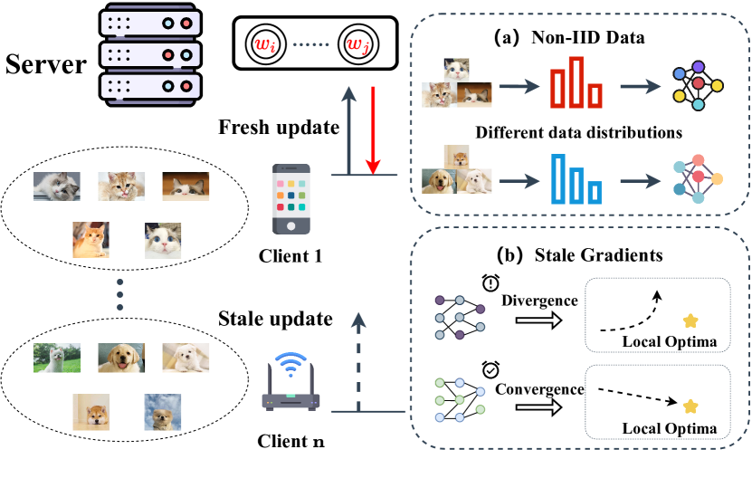
Figure 1: Problem illustration of K-async FL. (a) Non-IID data introduces biases among local gradients. This heterogeneity affects the convergence of the global model. (b) Stale gradients are often detrimental to the global model, causing update directions to deviate from local optima.

A well-known FL aggregation algorithm is federated averaging (FedAvg) (McMahan et al. 2017), where the server aggregates updates from a selected group of local clients and computes the global model by applying a weighted averaging strategy. Due to the system and statistical heterogeneity among devices, this approach often encounters the straggler effect (Cipar et al. 2013), which severely hampers the training progress. In response, (Xie, Koyejo, and Gupta 2019) introduced asynchronous FL (AFL), where the server no longer waits for all clients but can promptly update the global model upon receiving a single local gradient. However, AFL may lead to global model bias towards fast clients, and the frequent data transmissions may result in server crashes (Shi, Zhou, and Niu 2020). Some studies have tried to seek a compromise between synchronous and asynchronous approaches (Wu et al. 2020; Ma et al. 2021; Zhou et al. 2022), where K-async FL (Zhou et al. 2022) has demonstrated promising results, particularly in highly heterogeneous environments. In K-async FL, the server initiates aggregation as soon as it receives the first K local gradients, while the remaining clients continue their local training.

Despite the favorable performance of K-async FL, it is still constrained by two challenges, as shown in Figure 1. On the one hand, the presence of non-independent and identically distributed (Non-IID) data poses a significant challenge in training a well-performing global model (Zhao et al. 2018). On the other hand, the existence of stale local gradients often affects the utility of the global gradient, even leading to divergence (Zhang et al. 2023a). Currently, it is common practice to adopt strategies such as variance reduction (Karimireddy et al. 2020; Li, He, and Song 2021), regularization (Li et al. 2020), and momentum (Li et al. 2019; Xu and Huang 2022) to accommodate heterogeneous scenarios. As for the latter, the mainstream approach involves assigning different weights to local gradients based on their staleness (Chen, Sun, and Jin 2019; Damaskinos et al. 2022) to alleviate the weight divergence. While some algorithms can address both aforementioned issues simultaneously, they either rely on a sole weighted criterion (Zhou et al. 2022) leading to a biased allocation of weights, or necessitate specific prior knowledge that is not readily accessible such as the grouping of clients based on varying computational capacities (Li et al. 2022b), resulting in challenges in practical application.

To address these two challenges, we propose FedHist, a novel K-async FL framework that is capable of handling Non-IID data and stale gradients simultaneously. Specifically, we leverage a historical gradient buffer at the server-side to facilitate knowledge sharing across clients, enhancing the adaptability to Non-IID data. And we use the historical updates of clients to evaluate their utilities, as a factor for determining their weights during the near future aggregation stage. Additionally, we investigate factors that influence convergence and propose a strategy for amplifying the $\ell_{2}$-norms of aggregated gradients adaptively to accelerate the convergence of K-async FL. More importantly, FedHist does not require any prior knowledge about the clients, such as computational capabilities, and maintains the same level of privacy as FedAvg. In summary, with the aid of three core components, FedHist effectively addresses the challenges posed by Non-IID data and stale gradients in AFL. Our main contributions can be summarized as follows:

• We propose FedHist, a novel solution tailored for Non-IID data and stale gradients in AFL, deftly accommodating both of these challenges.

• We introduce a gradient buffer to achieve history-aware aggregation on the basis of improving the stability of local gradients and propose a $\ell_{2}$-norm amplification strategy. To the best of our knowledge, we are the first to propose using historical gradients to mirror client utility and expedite the future convergence process.

• Extensive experiments on public datasets demonstrate that FedHist significantly outperforms state-of-the-art methods. Furthermore, the ablation experiments validate the flexibility and scalability of FedHist.

Related Work and Motivation

Non-IID Data

Statistical heterogeneity refers to the variations in data distribution and data characteristics among individual clients, which has a significant impact on model performance (Chen et al. 2020; Li et al. 2022c). (Zhao et al. 2018) investigates the impact of Non-IID data on FL and observes that as data heterogeneity increases, the accuracy of the classical synchronous algorithm FedAvg diminishes. To mitigate such heterogeneity, some classical approaches involve introducing proximal regularization to reduce variance (Li et al. 2020; Karimireddy et al. 2020; Li, He, and Song 2021). Another intuitive approach is to leverage non-sensitive data to improve training efficiency (Zhang et al. 2022; Zhao et al. 2018) or directly distribute models across clients (Fan et al. 2022). Some studies employ the method of client selection (Lai et al. 2021; Nishio and Yonetani 2019; Li et al. 2022a) with the aim of prioritizing clients that possess higher statistical and system utility. However, these methods either yield only marginal performance improvements or require prior knowledge of the statistical characteristics of each client or rely on additional data, making their implementation challenging in many practical scenarios.

Gradient Staleness

Stale gradients often possess more noise, which may impede convergence speed and even lead to training failure, particularly in Non-IID data scenarios (Dai et al. 2018; Zhou et al. 2018; Zhang et al. 2015). Hence, it has become a consensus in the majority of works to establish a negative correlation between the aggregation weights and the degree of staleness (Jiang et al. 2017; Chen, Sun, and Jin 2019; Su and Li 2022). Also, client grouping (Zhang et al. 2023b; Li et al. 2022d; Wang et al. 2021) can mitigate the impact of the straggler effect. Unfortunately, stragglers may also hold valuable information that could contribute to the model convergence (Liu et al. 2021; Zhou et al. 2022). Hence, relying solely on staleness to assign weights to clients can lead to unfair weight distribution outcomes. Several approaches propose boosting factors to bias the weights towards stale gradients, typically calculated based on the extent of deviation between stale gradients and fresh gradients (Abdelmoniem et al. 2023; Su and Li 2022). (Damaskinos et al. 2022) utilizes the Bhattacharyya coefficient to capture the significance of each gradient, but this approach carries the risk of inadvertently exposing the label distribution of individual client data, potentially leading to privacy breaches.

Trade-off

There exists a fundamental contradiction between simultaneously addressing the issues of Non-IID data and gradient staleness (Zhou et al. 2022). This stems from the fact that resolving the former necessitates considering as many gradients as possible, while the latter requires selecting a minority of low-staleness gradients. These two strategies can be summarized as “more is better” and “quality over quantity”. The interaction among them propels us to propose a novel weighting scheme for aggregation, which involves exploring the utility of diverse gradients beyond staleness, to achieve a more comprehensive information utilization.

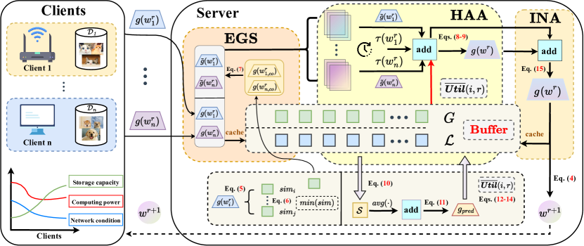
Figure 2: The overall framework of FedHist.

Methodology

FedHist tackles the challenges posed by Non-IID data and gradient staleness in K-async FL simultaneously through three fundamental components: enhancement of gradient stability, historical-aware aggregation, and intelligent $\ell_{2}$-norm amplification. Figure 2 illustrates the framework of FedHist.

Problem Statement

Suppose there are $N$ clients, denoted as $c_{1},c_{2},\ldots,c_{N}$. Each client $c_{i}$ trains a model using its local dataset $\mathcal{D}_{i}=\{\xi_{i,1},\xi_{i,2},\cdots,\xi_{i,\lvert{\mathcal{D}_{i}}\rvert}\}$, where $\xi_{i,j}$ represents the $j$-th data point $\{x_{j},y_{j}\}$ on client $i$. Our objective is to collaboratively train a global model $w$ using the entire dataset $\mathcal{D}=\bigcup_{i\in N}\mathcal{D}_{i}$ without compromising the privacy of the raw data. For client $c_{i}$, its empirical loss is defined as:

$$F_{i}(w)\triangleq\frac{1}{\lvert\mathcal{D}_{i}\lvert}\sum_{\xi_{i,j}\in\mathcal{D}_{i}}f(w,\xi_{i,j}),$$ (1)

where $w$ is a parameter vector, which is typically synchronized with the server at the beginning of each round, and $f(\cdot)$ is a loss function. The objective is to solve:

$$\underset{w}{arg\,min}\,F(w)\triangleq\sum_{i=1}^{K}\frac{\lvert\mathcal{D}_{i}\lvert}{\lvert\mathcal{D}\lvert}F_{i}(w),$$ (2)

where $K$ represents the number of participating clients in each communication round. In round $r+1$, client $c_{i}$ updates the parameter vector $w_{i}^{r}$ through mini-batch stochastic gradient descent (SGD) to minimize the objective function by Eq. (3):

$$w_{i}^{r+1}=w^{r}-\eta_{i}\nabla F_{i}(w^{r}),$$ (3)

where $w_{i}^{r+1}$ represents the model of client $c_{i}$ in round $r+1$, $w^{r}$ denotes the global model in round $r$, and $\eta_{i}$ represents the learning rate of client $c_{i}$. We use $g(w_{i}^{r})$ to denote the gradient submitted by $i$-th client in round $r$. Upon receiving $K$ gradients, the server updates the global model parameters by Eq. (4) accordingly:

$$w^{r+1}=w^{r}-\eta\sum_{i=1}^{K}p_{i}^{r}g(w_{i}^{r}).$$ (4)

Here, $w^{r+1}$ represents the global model in round $r+1$, $\eta$ denotes the learning rate of the server, $p_{i}^{r}$ denotes the weight of $i$-th client in round $r$, and $\sum_{i=1}^{K}p_{i}=1$, generally.

Enhancement of Gradient Stability (EGS)

FedHist integrates a buffer at the server-side that dynamically maintains the most recent historical gradients. This buffer is further divided into two fixed-length lists, denoted as $\mathcal{G}$ and $\mathcal{L}$, caching the global gradients and local gradients from the most recent $h$ communication rounds, respectively. And gradients from even earlier rounds will be cleared.

The goal of $\mathbf{EGS}$ is to select an appropriate collaboration gradient from $\mathcal{G}$ for each local gradient uploaded from the client, and then execute a weighted aggregation process. Quantitatively measuring the degree of similarity between two gradient vectors $g(w_{i})$ and $g(w_{j})$ can be achieved by computing their cosine similarity, as shown in Eq. (5):

$$cos\langle g(w_{i}),g(w_{j})\rangle=\frac{{g(w_{i})}\cdot{g(w_{j})}}{\|{g(w_{i})}\|\,\|{g(w_{j})}\|}.$$ (5)

We select the corresponding collaborative gradient for each local gradient based on the principle of minimizing similarity, as it implies a higher potential of sharing knowledge between two gradients and avoids overfitting (Hu et al. 2022). This fine-grained cross-aggregation method mitigates gradient divergence and rectifies bias in local gradients. Thus the objective is to find the optimal collaborative gradient $g(w_{i,co}^{r})$ for each $g(w_{i}^{r})$ by Eq. (6):

$$\underset{g(w)\in\mathcal{G}}{arg\,min}\;cos\langle g(w_{i}^{r}),g(w)\rangle.$$ (6)

The local gradient $g(w_{i}^{r})$ is fused with the collaborative gradient $g(w_{i,co}^{r})$ to enhance the diversity by Eq. (7):

$$\tilde{g}(w_{i}^{r})=g(w_{i}^{r})+\alpha\,g(w_{i,co}^{r}),$$ (7)

where $\tilde{g}(w_{i}^{r})$ represents the local gradient after incorporating historical experiences, which will be utilized in the subsequent aggregation phase, and $\alpha\,\textgreater\,0$ is a constant. Based on this, $\mathbf{EGS}$ alleviates client-drift by appropriately selecting a suitable collaborative historical global gradient for each local gradient, thereby enhancing its stability.

History-Aware Aggregation (HAA)

During the aggregation phase, while reducing the weight of highly stale gradients is necessary, it is crucial to identify contributors that potentially possess more valuable data and allocate appropriate additional weights to them. In light of this, $\mathbf{HAA}$ introduces a boosting factor to allocate the clients exhibiting superior performance in historical aggregations with higher weights. We combine the boosting factor with the exponential weighting method derived from (Chen, Sun, and Jin 2019) and control the weights of these two components using a constant $\lambda$, as shown in Eq. (8):

$$\hat{p}_{i}^{r}=\sum_{i=1}^{K}\left(\left(\frac{e}{2}\right)^{-\tau(w_{i}^{r})}+\lambda\cdot\overline{\boldsymbol{Util}}{(i,r)}\right),$$ (8)

where $\tau(w_{i}^{r})$ and $\overline{\boldsymbol{Util}}{(i,r)}$ represent the staleness and the utility value of the $i$-th client in round $r$, respectively. $\tau(w_{i}^{r})\geq 1$ indicates the number of communication rounds experienced by the client from receiving the global model to uploading its update and $\overline{\boldsymbol{Util}}{(i,r)}$ is obtained based on its historical behavior. Then, $\hat{p}_{i}^{r}$ needs to be normalized:

$${p}_{i}^{r}=\frac{\hat{p}_{i}^{r}}{\sum_{i=1}^{K}\hat{p}_{i}^{r}}.$$ (9)

A pivotal step involves the computation of the utility value $\overline{\boldsymbol{Util}}$, and $\mathbf{HAA}$ obtains it by identifying relatively fresh updates and generating predicted unbiased gradients for client utility evaluation, as outlined below.

Relatively fresh updates.

By configuring a historical buffer on the server-side, in round $r$, the server can trace back to historical gradients up to round $r-h$, thereby enabling the identification of relatively fresh updates. The so-called relatively fresh update refers to a gradient whose staleness is $h+1$ in round $r$, while its staleness is $1$ relative to round $r-h$. In other words, although it may be considered stale in round $r$, it is relatively fresh to round $r-h$. After the completion of each communication round, the server retrieves all local gradients from $\mathcal{L}$ within the buffer and stores all the gradients that satisfy Eq. (10) into a pre-cleared set $\mathcal{S}$.

$$g_{L}\in\mathcal{L}\quad\text{s.t.} \tau(g_{L})=\text{index}(g_{L},\mathcal{L})+1,$$ (10)

$$0\leq\text{index}(g_{L},\mathcal{L})\leq h-1.$$

Here, $\text{index}(g_{L},\mathcal{L})$ denotes the index of the sublist containing $g_{L}$ within $\mathcal{L}$. Based on this, in round $r$, we are able to obtain all the relatively fresh updates to round $r-h$, and then we can obtain the predicted unbiased gradient.

Predicted unbiased gradients.

Since the local gradients in $\mathcal{S}$ are relatively fresh to round $r-h$, their aggregated result has higher credibility to the global gradient in round $r-h$. By performing average aggregation on them, a predicted unbiased gradient $g_{pred}$ can be generated, representing the ideal global gradient obtained in the absence of staleness scenarios in round $r-h$.

$$g_{pred}\triangleq\frac{1}{\lvert\mathcal{S}\lvert}\sum_{g(w)\in\mathcal{S}}g(w).$$ (11)

Note that the actual global gradient $g_{act}$ in round $r-h$, i.e., $g(w^{w-h})$, is still formed by aggregating those potentially stale local gradients. In fact, it is staleness that leads to the deviation between $g_{act}$ and $g_{pred}$. In order to assess the quality of the local gradients in round $r-h$, we can calculate their similarity with $g_{pred}$ one by one, followed by the corresponding client utility evaluation.

Client utility evaluation.

At the end of each communication round $r$, the server evaluates the historical local gradients (referred to as $g_{his}^{i}$ hereafter for simplicity) participating in the aggregation phase in round $r-h$. $\mathbf{HAA}$ evaluates the utility of the corresponding client using Eqs. (12) - (13).

$$\boldsymbol{Util}(i,r)=(cos\langle g_{his}^{i},g_{pred}\rangle-sim_{thr})\cdot p_{his}^{i}\cdot\lvert\mathcal{S}\lvert,$$ (12)

where $sim_{thr}$ is a similarity threshold, and $p_{his}^{i}$ is determined based on the actual (not relative) staleness of $g_{his}^{i}$:

$$p_{his}^{i}=\begin{cases}(1-e\,/\,2)^{-\tau(g_{his}^{i})}&\\ \qquad\qquad\mathbf{if}\quad cos\langle g_{his}^{i},g_{pred}\rangle\geq sim_{thr};\\ (e\,/\,2)^{-\tau(g_{his}^{i})}&\\ \qquad\qquad\mathbf{if}\quad cos\langle g_{his}^{i},g_{pred}\rangle<sim_{thr}.\end{cases}$$ (13)

According to Eqs. (12) - (13), the sign of $\boldsymbol{Util}(i,r)$ depends on whether the similarity exceeds the threshold (i.e., reward or penalty). If a gradient has a higher staleness during the actual aggregation process, it is expected to exhibit lower similarity with $g_{pred}$, thereby deserving relatively higher rewards or lower penalties, and vice versa. Moreover, the number of gradients in $\mathcal{S}$ reflects the predictive accuracy of $g_{pred}$, thus $\boldsymbol{Util}$ is positively correlated with $\lvert\mathcal{S}|$. To mitigate the influence of data noise, we employ an exponential moving average with a constant $\gamma$ to obtain the average utility $\overline{\boldsymbol{Util}}{(i,r)}$.

$$\overline{\boldsymbol{Util}}{(i,r)}=(1-\gamma)\cdot\overline{\boldsymbol{Util}}{(i,r-1)}+\gamma\cdot\boldsymbol{Util}(i,r).$$ (14)

By applying Eqs. (9) - (14) to Eq. (8), $\mathbf{HAA}$ employs a multi-dimensional weighting method by leveraging the participants’ historical updates, emphasizing the gradients from clients with more valuable data, even if they are stale.

Algorithm 1 Federated Historical Learning $($FedHist$)$

1:communication rounds $R$, number of gradients received by server $K$, learning rate $\eta$, length of the server-side buffer $h$, constant $\alpha,\lambda,\gamma,\mu$.

2:Optimal solution $w^{*}$.

3:Initialization.

4:for each communication round $r$ = $1,\ldots,R$ do

5:     for $i=1$ to $K$ do in parallel

6:         Receive $\{g(w_{i}^{r})$$,\tau(w_{i}^{r}\}$ from the $i$-th client.

7:         $\mathcal{L}[h-1]\leftarrow\mathcal{L}[h-1]+[g(w_{i}^{r})]$

8:         if $r\textgreater h$ then $\triangleright$ EGS

9:              Calculate $g(w_{i,co}^{r})$ according to Eq. (6).

10:              $\tilde{g}(w_{i}^{r})\leftarrow g(w_{i}^{r})+\alpha\cdot g(w_{i,co}^{r})$.

11:         else

12:              $\tilde{g}(w_{i}^{r})\leftarrow g(w_{i}^{r})$.

13:         end if

14:     end for

15:     Calculate $p_{i}^{r}$ for $i=1$ to $K$ by Eqs.(8) - (9).$\triangleright$ HAA

16:     $g(w^{r})\leftarrow\sum_{i=1}^{K}p_{i}^{r}g(w_{i}^{r})$.

17:     Adjust the $\ell_{2}$-norm of ${g}(w^{r})$ by Eq. (15).$\triangleright$ INA

18:     Update global model $w^{r}$ by Eq. (4).

19:     Distribute $w^{r}$ to the participants.

20:     Calculate $g_{pred}$ by Eqs. (10) - (11).

21:     Update $\overline{\boldsymbol{Util}}$ by Eqs. (12) - (14).

22:     $\mathcal{L}\leftarrow\mathcal{L}[1:]+[\,[\;]\,]$.$\triangleright$ Update the buffer

23:     $\mathcal{G}\leftarrow\mathcal{G}[1:]+[{g}(w^{r})]$.$\triangleright$ Cache the global model

24:end for

Intelligent $\ell_{2}$-Norm Amplification (INA)

Due to the impact of Non-IID data, notable biases exist among the local gradients, thus the aggregated gradient typically exhibits a relatively lower $\ell_{2}$-norm, leading to quite limited improvements at each iteration and significantly hindering the convergence speed. An intuitive approach is to make the $\ell_{2}$-norm of the aggregated gradient comparable to that of the local gradients involved in the aggregation. Thus we enhance the convergence speed and stability by Eq. (15):

$$\|g(w^{r})\|_{2}=\frac{1-\mu\cdot r}{K}\sum_{i=1}^{K}\|g(w_{i}^{r})\|_{2},$$ (15)

where $r$ represents the current communication round and $\mu\in(0,\frac{1}{r})$ is a constant. Eq. (15) modifies the $\ell_{2}$-norm of the aggregated result to match the average $\ell_{2}$-norm of all local gradients before aggregation, and it decreases as the training progresses. This adjustment empowers $\mathbf{INA}$ to prevent significant reductions in the $\ell_{2}$-norm of the aggregated result. Generally, a larger $\ell_{2}$-norm of gradient implies the presence of more knowledge, and the $\ell_{2}$-norm of gradient learned from the previously trained samples tend to be relatively smaller (Shin et al. 2022). Thus, in addition to smoothing the convergence process, $\mathbf{INA}$ also possesses the capability of perceiving the significance of updates.

Pipeline of FedHist

Algorithm 1 summarizes the pipeline of the server-side of FedHist. Initially, the server receives and caches the first $K$ local gradients (Lines 4-5), followed by the application of $\mathbf{EGS}$ to enhance their stability (Lines 6-8). Subsequently, the server obtains the utility value $\overline{\boldsymbol{Util}}$ through $\mathbf{HAA}$ and aggregates the $K$ local gradients, considering their staleness (Lines 13-14), followed by $\ell_{2}$-norm adjustment performed by $\mathbf{INA}$ (Line 15). After the server finishes updating the global model (Line 16) and distributes it to the participants (Line 17), it computes the utility value $\overline{\boldsymbol{Util}}$ of the clients participating in round $r-h$ (Lines 18-19) and then maintains a fixed length of the buffer (Lines 20-21).

Staleness	Methods	FMNIST			CIFAR10			CIFAR100
		$\beta=0.3$	$\beta=1.0$	IID	$\beta=0.3$	$\beta=1.0$	IID	$\beta=0.3$	$\beta=1.0$	IID
$N/K=10$	FedAvg	70.93	76.09	79.45	51.39	57.66	61.47	27.80	28.57	29.21
	FedProx	71.28	76.82	79.18	52.41	56.89	61.84	28.10	28.43	30.75
	MOON	71.72	76.39	79.35	52.08	57.50	61.39	27.90	29.77	30.34
	DynSGD	71.89	76.05	79.58	52.02	57.90	62.11	27.75	29.06	30.33
	REFL	72.31	77.47	79.88	51.67	57.72	61.76	28.34	28.77	29.03
	TWAFL	72.44	74.67	79.48	51.43	57.71	61.91	27.27	29.26	29.73
	WKAFL	73.45	77.92	80.04	54.76	58.44	62.26	27.72	28.33	29.64
	FedHist	78.05	81.34	83.29	57.19	59.78	62.66	28.78	29.89	30.90
$N/K=100$	FedAvg	70.24	72.05	74.41	44.35	52.26	55.27	23.49	25.47	24.81
	FedProx	71.01	72.40	74.11	43.21	49.60	55.98	24.65	24.74	24.65
	MOON	71.79	74.94	75.85	41.59	50.72	53.57	23.10	22.69	22.77
	DynSGD	72.29	73.39	76.06	51.11	55.33	57.25	24.91	26.14	26.31
	REFL	70.98	75.67	77.28	51.46	54.80	57.11	25.22	25.76	26.44
	TWAFL	72.73	73.27	75.31	47.16	53.00	55.87	23.53	23.91	24.57
	WKAFL	70.56	75.37	74.97	45.60	51.42	55.01	22.57	23.64	24.82
	FedHist	74.49	77.28	78.44	52.03	55.92	58.61	25.78	26.31	26.70

Table 1: Test Accuracy (%) when using FedHist and baselines on FMNIST, CIFAR-10, and CIFAR-100 Datasets. $N/K$ is considered at two different levels: 10 and 100, to assess different degrees of staleness. $\beta$ represents the degree of data heterogeneity, taking values of 0.3, 1.0, and $\infty$. The best result in each column is shown in bold and the second-best is underlined.

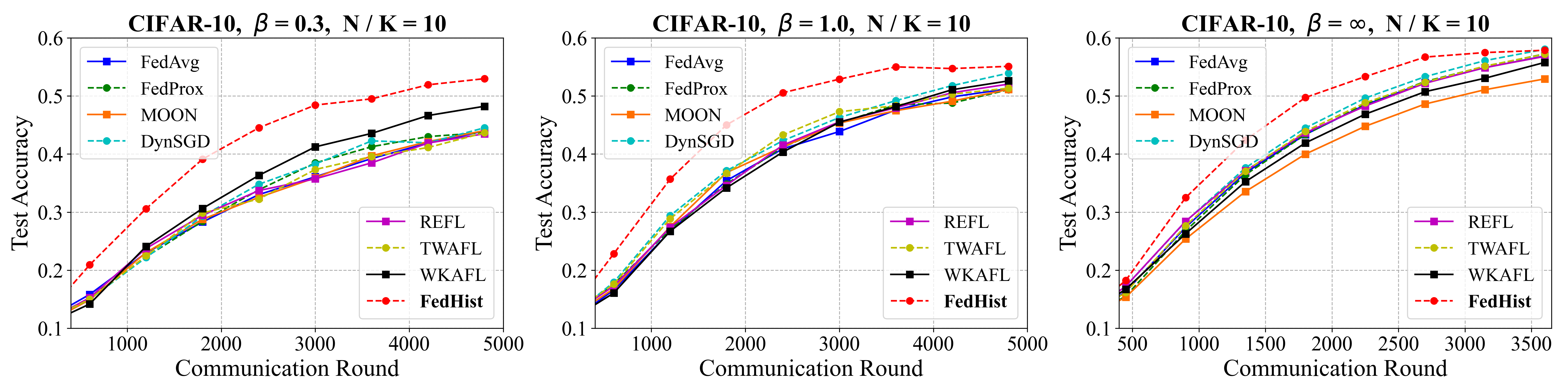
Figure 3: Performance of FedHist and baselines during the training process on CIFAR-10 with $\beta$ = 0.3, 1.0 and $\infty$.

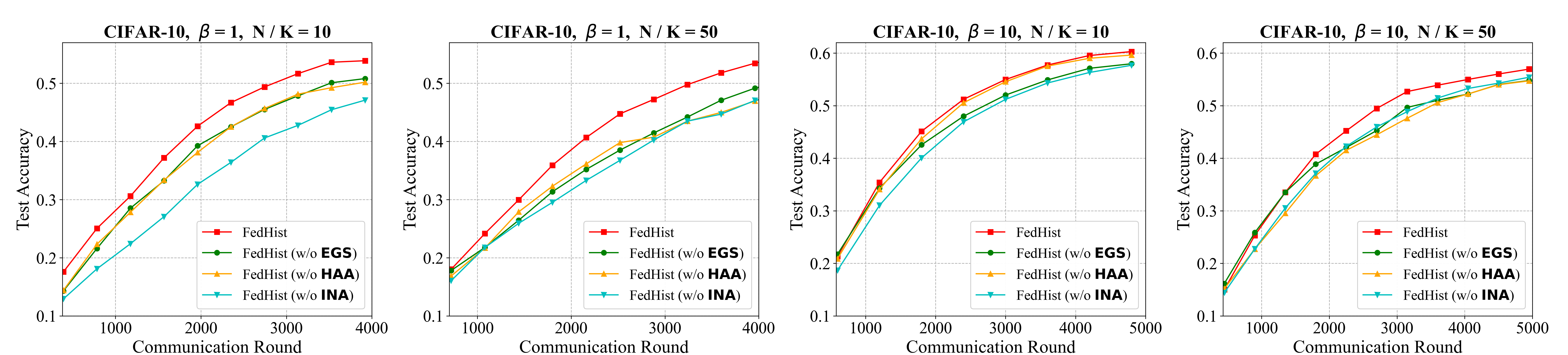
Figure 4: Performance of FedHist with different missing components on CIFAR-10.

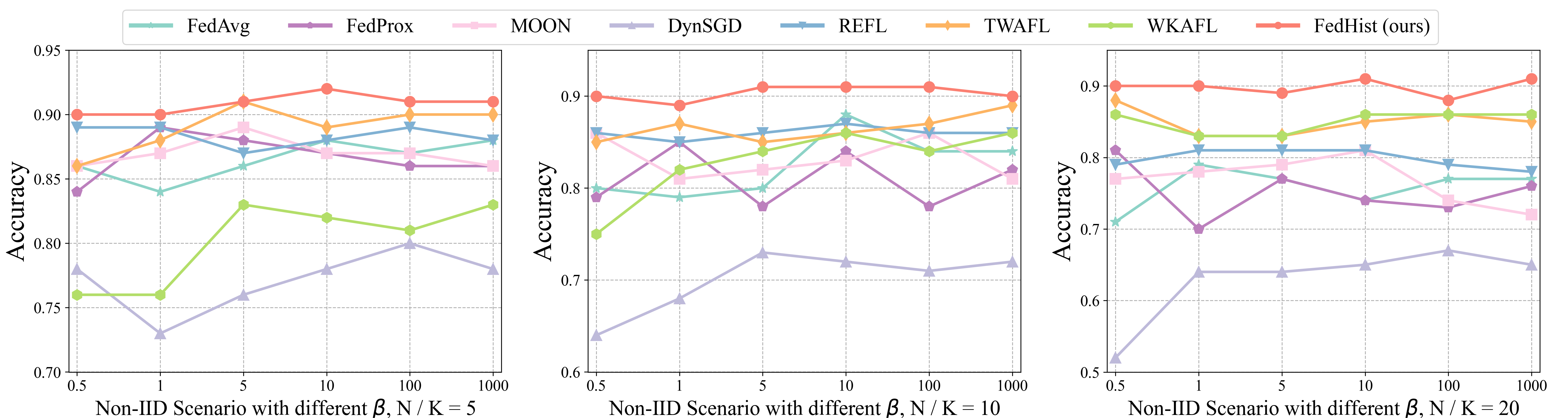
Figure 5: Performance of FedHist and baselines on FMNIST with specific labels occurring only on a few slow clients.

Experiments

Experimental Settings

Datasets and models.

Our experiments are conducted on 3 well-known datasets, including CIFAR-10, CIFAR-100 (Krizhevsky, Hinton et al. 2009), and Fashion MNIST (FMNIST) (Xiao, Rasul, and Vollgraf 2017). To better simulate real-world scenarios of IID and Non-IID data, we employ the Dirichlet distribution $Dir_{N}(\beta)$ (Hsu, Qi, and Brown 2019) to divide the dataset. Here, $\beta$ controls the degree of data heterogeneity, where a smaller $\beta$ signifies a more pronounced imbalance in the quantity and labels of samples among clients. Besides, we introduce different levels of staleness by setting $N/K$ (the ratio of the number of total clients to the participants in each round). This choice stems from a theorem stating that the minimum average staleness is approximately equal to $N/(2K)$ (Zhou et al. 2022). And all experiments are conducted using LeNet (LeCun et al. 1998).

Baselines.

We select several relevant algorithms for comparison: FedAvg (McMahan et al. 2017), DynSGD (Jiang et al. 2017), TWAFL (Chen, Sun, and Jin 2019), FedProx (Li et al. 2020), MOON (Li, He, and Song 2021), WKAFL (Zhou et al. 2022) and REFL (Abdelmoniem et al. 2023). While some of them were initially proposed for synchronous FL, we also acknowledge their potential to support asynchronous scenarios through simple modifications. Please refer to Appendix A, B for more details of settings and results.

Performance Comparison

Data heterogeneity.

Table 2 and Figure 3 illustrate that FedHist exhibits faster convergence rates compared to the baselines across three levels of heterogeneity, while also demonstrating the highest test accuracy, especially in highly heterogeneous environments. This is mainly attributed to the $\mathbf{EGS}$ within FedHist, which enhances the stability of local gradients and mitigates the impact of Non-IID data. Moreover, it is evident that the test accuracy of all methods improves with the increase of $\beta$, highlighting the detrimental impact of data heterogeneity on the training process.

Degrees of staleness.

Table 2 demonstrates the leading test accuracy of FedHist across various staleness levels. Although the test accuracy of all methods experiences a certain decline with the increase of $N/K$, the incorporation of the $\mathbf{HAA}$ in FedHist comprehensively considers the utility of client updates, thereby enabling its adaptability in highly stale environments and satisfactory robustness to staleness. Furthermore, WKAFL, REFL, and TWAFL achieve relatively commendable results owing to their concerted efforts in coping with staleness, while FedAvg performs the least favorably due to its lack of measures to address staleness.

Convergence speed.

Table 2 demonstrates that to achieve the target accuracy (40%), FedHist achieves an acceleration ratio of approximately 1.8$\times$-2.0$\times$ compared to FedAvg, surpassing all baselines. The convergence trends of different methods displayed in Figure 3 intuitively highlight the advantages of FedHist in diverse data heterogeneity settings. More importantly, FedHist consistently gains a significant advantage in the early stages of training, and its convergence curve remains smoother. This is achieved by adaptively amplifying the $\ell_{2}$-norms of aggregated gradients through $\mathbf{INA}$.

Methods	$\beta$ = 0.3		$\beta$ = 1		$\beta$ = $\infty$
	R#	S $\uparrow$	R#	S $\uparrow$	R#	S $\uparrow$
FedAvg	3340	1×	2182	1×	1391	1×
FedProx	3876	0.9×	2370	0.9×	1562	0.9×
MOON	4324	0.8×	2088	1.0×	1444	1.0×
DynSGD	1904	1.8×	1573	1.4×	1176	1.2×
REFL	2177	1.5×	1289	1.7×	1013	1.4×
TWAFL	2695	1.2×	1492	1.5×	1244	1.1×
WKAFL	2954	1.1×	1701	1.3×	1299	1.1×
FedHist	1754	1.9×	1089	2.0×	792	1.8×

Table 2: Communication rounds in different methods to achieve target accuracy (40%) on CIFAR-10. R# represents the required number of communication rounds and S $\uparrow$ is the corresponding convergence speedup relative to FedAvg.

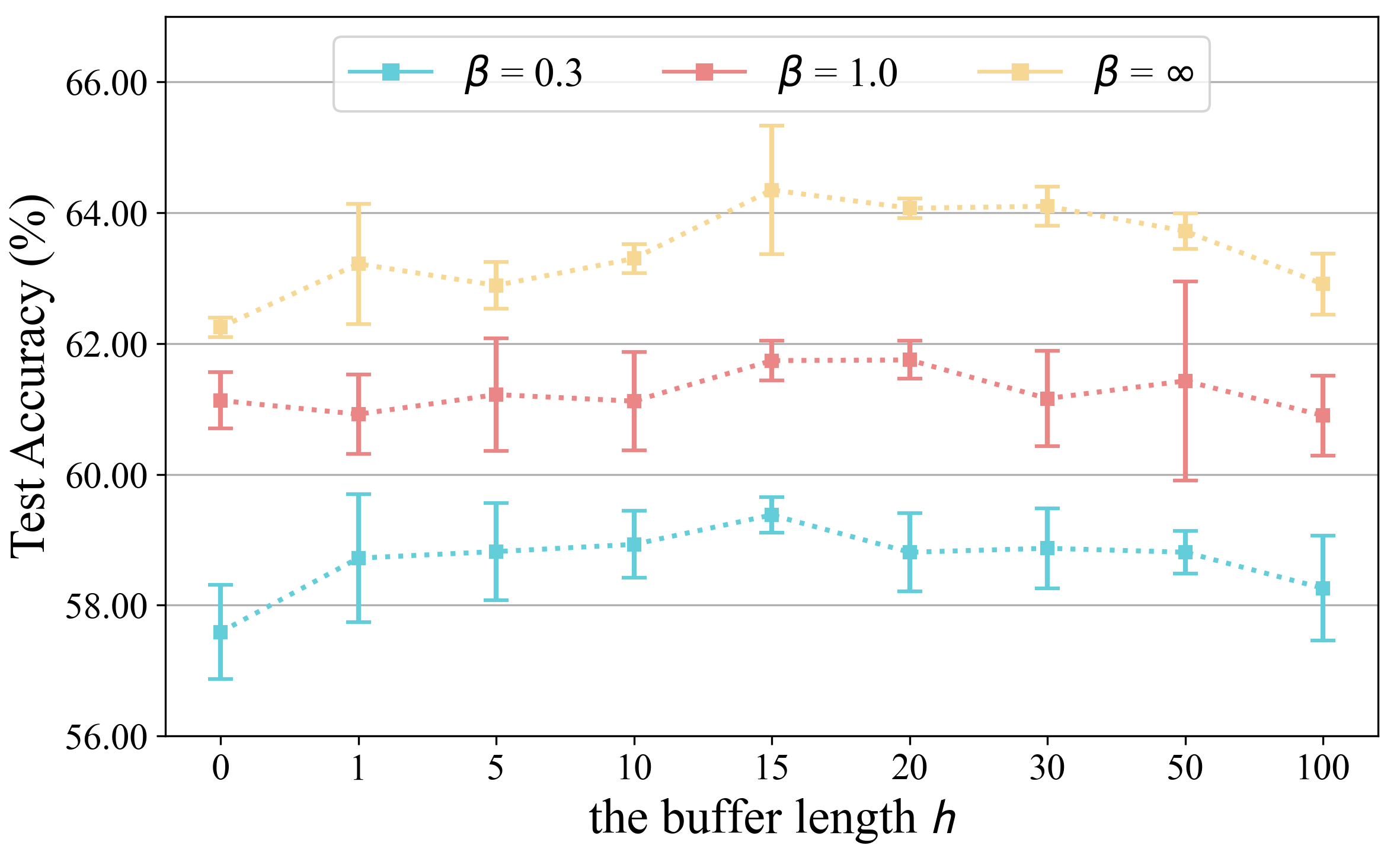
Figure 6: Performance of FedHist with different $h$.

Model Analysis

Ablation studies.

To further investigate the effectiveness of each component of FedHist, we conduct ablation studies, as shown in Figure 4. We systematically remove each of the three core components of FedHist and denote it as w/o (without) to indicate the absence of that particular component. The results demonstrate that regardless of the various data heterogeneities or different model staleness scenarios, FedHist consistently exhibits rapid convergence capability and stability. Indeed, the inferior stability observed in FedHist (w/o $\mathbf{EGS}$) and FedHist (w/o $\mathbf{HAA}$) indicates the impact of Non-IID data and staleness leads to the deviation of local gradients, hinders the convergence of the global model. Also, the slower convergence speed observed in FedHist (w/o $\mathbf{INA}$) reflects the effectiveness of the $\ell_{2}$-norm amplification strategy. More details please refer to Appendix C.

Sensitivity of the buffer length.

We further analyze the impact of the buffer length $h$ on FedHist concerning different degrees of statistical heterogeneity. As shown in Figure 6, we plot the average test accuracy of the global model with standard deviation by searching $h$ $\in$ {0, 1, 5, 10, 15, 20, 30, 50, 100}. Figure 6 shows that a larger $h$ results in performance degradation due to the significantly reduced value of utilizing gradients cached in the buffer for an extended period, thus causing the collaborative gradient selected by $\mathbf{EGS}$ to compromise the stability of local gradients, and a smaller $h$ would lead to reduced predictive reliability of $\mathbf{HAA}$. Especially, the inferior performance when $h$ = 1 highlights the superiority of FedHist over momentum-based approaches (Hsu, Qi, and Brown 2019; Li et al. 2019).

Impacts of the boosting factor.

To validate the capability of FedHist in handling extremely heterogeneous scenarios, we conduct an experiment by setting the tenth class samples (for a 10-class classification task) to occur only in a small fraction of slow clients with an update frequency of 50% compared to normal clients, and compare the experimental results of all the methods. As shown in Figure 5, FedHist demonstrates the highest test accuracy for these samples, which remains unaffected by changes in different degrees of data heterogeneity or staleness. This can be attributed to its consideration of aggregation weights beyond staleness. Through this multi-dimensional weighting approach, FedHist is capable of adapting to extremely heterogeneous scenarios. Please refer to Appendix D for more details.

Conclusion

In this work, we propose federated historical learning (FedHist), a novel asynchronous FL method that utilizes the server-side buffer to replay the knowledge of historical gradients and mirror the utility of clients. FedHist first enhances the stability of local gradients by fine-grained cross-aggregation with historical global gradients. Moreover, it assigns the aggregation weights in a multi-dimensional manner based on the utility and staleness of the clients and enables fast and stable convergence by adjusting the $\ell_{2}$-norm of the aggregated gradient. We conduct extensive experiments on public datasets and validate the effectiveness of FedHist in addressing the challenges posed by both Non-IID data and gradient staleness, simultaneously.

References

- Abdelmoniem et al. (2023) Abdelmoniem, A. M.; Sahu, A. N.; Canini, M.; and Fahmy, S. A. 2023. REFL: Resource-Efficient Federated Learning. In Proceedings of the Eighteenth European Conference on Computer Systems, 215–232.
- Brisimi et al. (2018) Brisimi, T. S.; Chen, R.; Mela, T.; Olshevsky, A.; Paschalidis, I. C.; and Shi, W. 2018. Federated learning of predictive models from federated electronic health records. International journal of medical informatics, 112: 59–67.
- Chen et al. (2020) Chen, Y.; Ning, Y.; Slawski, M.; and Rangwala, H. 2020. Asynchronous online federated learning for edge devices with non-iid data. In 2020 IEEE International Conference on Big Data (Big Data), 15–24. IEEE.
- Chen, Sun, and Jin (2019) Chen, Y.; Sun, X.; and Jin, Y. 2019. Communication-efficient federated deep learning with layerwise asynchronous model update and temporally weighted aggregation. IEEE transactions on neural networks and learning systems, 31(10): 4229–4238.
- Cipar et al. (2013) Cipar, J.; Ho, Q.; Kim, J. K.; Lee, S.; Ganger, G. R.; Gibson, G.; Keeton, K.; and P Xing, E. 2013. Solving the straggler problem with bounded staleness.
- Dai et al. (2018) Dai, W.; Zhou, Y.; Dong, N.; Zhang, H.; and Xing, E. P. 2018. Toward understanding the impact of staleness in distributed machine learning. arXiv preprint arXiv:1810.03264.
- Damaskinos et al. (2022) Damaskinos, G.; Guerraoui, R.; Kermarrec, A.-M.; Nitu, V.; Patra, R.; and Taiani, F. 2022. Fleet: Online federated learning via staleness awareness and performance prediction. ACM Transactions on Intelligent Systems and Technology (TIST), 13(5): 1–30.
- Fan et al. (2022) Fan, Z.; Wang, Y.; Yao, J.; Lyu, L.; Zhang, Y.; and Tian, Q. 2022. Fedskip: Combatting statistical heterogeneity with federated skip aggregation. In 2022 IEEE International Conference on Data Mining (ICDM), 131–140. IEEE.
- Hard et al. (2018) Hard, A.; Rao, K.; Mathews, R.; Ramaswamy, S.; Beaufays, F.; Augenstein, S.; Eichner, H.; Kiddon, C.; and Ramage, D. 2018. Federated learning for mobile keyboard prediction. arXiv preprint arXiv:1811.03604.
- Hsu, Qi, and Brown (2019) Hsu, T.-M. H.; Qi, H.; and Brown, M. 2019. Measuring the effects of non-identical data distribution for federated visual classification. arXiv preprint arXiv:1909.06335.
- Hu et al. (2022) Hu, M.; Zhou, P.; Yue, Z.; Ling, Z.; Huang, Y.; Liu, Y.; and Chen, M. 2022. FedCross: Towards Accurate Federated Learning via Multi-Model Cross Aggregation. arXiv preprint arXiv:2210.08285.
- Jiang et al. (2017) Jiang, J.; Cui, B.; Zhang, C.; and Yu, L. 2017. Heterogeneity-aware distributed parameter servers. In Proceedings of the 2017 ACM International Conference on Management of Data, 463–478.
- Karimireddy et al. (2020) Karimireddy, S. P.; Kale, S.; Mohri, M.; Reddi, S.; Stich, S.; and Suresh, A. T. 2020. Scaffold: Stochastic controlled averaging for federated learning. In International Conference on Machine Learning, 5132–5143. PMLR.
- Konečnỳ et al. (2016) Konečnỳ, J.; McMahan, H. B.; Yu, F. X.; Richtárik, P.; Suresh, A. T.; and Bacon, D. 2016. Federated learning: Strategies for improving communication efficiency. arXiv preprint arXiv:1610.05492.
- Krizhevsky, Hinton et al. (2009) Krizhevsky, A.; Hinton, G.; et al. 2009. Learning multiple layers of features from tiny images.
- Lai et al. (2021) Lai, F.; Zhu, X.; Madhyastha, H. V.; and Chowdhury, M. 2021. Oort: Efficient federated learning via guided participant selection. In 15th USENIX Symposium on Operating Systems Design and Implementation (OSDI 21), 19–35.
- LeCun et al. (1998) LeCun, Y.; Bottou, L.; Bengio, Y.; and Haffner, P. 1998. Gradient-based learning applied to document recognition. Proceedings of the IEEE, 86(11): 2278–2324.
- Li et al. (2019) Li, C.; Li, R.; Wang, H.; Li, Y.; Zhou, P.; Guo, S.; and Li, K. 2019. Gradient scheduling with global momentum for non-iid data distributed asynchronous training. arXiv preprint arXiv:1902.07848.
- Li et al. (2022a) Li, C.; Zeng, X.; Zhang, M.; and Cao, Z. 2022a. PyramidFL: A fine-grained client selection framework for efficient federated learning. In Proceedings of the 28th Annual International Conference on Mobile Computing And Networking, 158–171.
- Li et al. (2022b) Li, G.; Hu, Y.; Zhang, M.; Liu, J.; Yin, Q.; Peng, Y.; and Dou, D. 2022b. FedHiSyn: A hierarchical synchronous federated learning framework for resource and data heterogeneity. In Proceedings of the 51st International Conference on Parallel Processing, 1–11.
- Li et al. (2022c) Li, Q.; Diao, Y.; Chen, Q.; and He, B. 2022c. Federated learning on non-iid data silos: An experimental study. In 2022 IEEE 38th International Conference on Data Engineering (ICDE), 965–978. IEEE.
- Li, He, and Song (2021) Li, Q.; He, B.; and Song, D. 2021. Model-contrastive federated learning. In Proceedings of the IEEE/CVF conference on computer vision and pattern recognition, 10713–10722.
- Li et al. (2020) Li, T.; Sahu, A. K.; Zaheer, M.; Sanjabi, M.; Talwalkar, A.; and Smith, V. 2020. Federated optimization in heterogeneous networks. Proceedings of Machine learning and systems, 2: 429–450.
- Li et al. (2022d) Li, Z.; Huang, C.; Gai, K.; Lu, Z.; Wu, J.; Chen, L.; Xu, Y.; and Choo, K.-K. R. 2022d. AsyFed: Accelerate Federated Learning with Asynchronous Communication Mechanism. IEEE Internet of Things Journal.
- Liang et al. (2022) Liang, X.; Liu, Y.; Chen, T.; Liu, M.; and Yang, Q. 2022. Federated transfer reinforcement learning for autonomous driving. In Federated and Transfer Learning, 357–371. Springer.
- Liu et al. (2021) Liu, J.; Wang, J. H.; Rong, C.; Xu, Y.; Yu, T.; and Wang, J. 2021. FedPA: An adaptively partial model aggregation strategy in Federated Learning. Computer Networks, 199: 108468.
- Ma et al. (2021) Ma, Q.; Xu, Y.; Xu, H.; Jiang, Z.; Huang, L.; and Huang, H. 2021. FedSA: A semi-asynchronous federated learning mechanism in heterogeneous edge computing. IEEE Journal on Selected Areas in Communications, 39(12): 3654–3672.
- McMahan et al. (2017) McMahan, B.; Moore, E.; Ramage, D.; Hampson, S.; and y Arcas, B. A. 2017. Communication-efficient learning of deep networks from decentralized data. In Artificial intelligence and statistics, 1273–1282. PMLR.
- Nishio and Yonetani (2019) Nishio, T.; and Yonetani, R. 2019. Client selection for federated learning with heterogeneous resources in mobile edge. In ICC 2019-2019 IEEE international conference on communications (ICC), 1–7. IEEE.
- Shi, Zhou, and Niu (2020) Shi, W.; Zhou, S.; and Niu, Z. 2020. Device scheduling with fast convergence for wireless federated learning. In ICC 2020-2020 IEEE International Conference on Communications (ICC), 1–6. IEEE.
- Shin et al. (2022) Shin, J.; Li, Y.; Liu, Y.; and Lee, S.-J. 2022. FedBalancer: data and pace control for efficient federated learning on heterogeneous clients. In Proceedings of the 20th Annual International Conference on Mobile Systems, Applications and Services, 436–449.
- Su and Li (2022) Su, N.; and Li, B. 2022. How Asynchronous can Federated Learning Be? In 2022 IEEE/ACM 30th International Symposium on Quality of Service (IWQoS), 1–11. IEEE.
- Wang et al. (2021) Wang, Z.; Xu, H.; Liu, J.; Huang, H.; Qiao, C.; and Zhao, Y. 2021. Resource-efficient federated learning with hierarchical aggregation in edge computing. In IEEE INFOCOM 2021-IEEE Conference on Computer Communications, 1–10. IEEE.
- Wu et al. (2020) Wu, W.; He, L.; Lin, W.; Mao, R.; Maple, C.; and Jarvis, S. 2020. SAFA: A semi-asynchronous protocol for fast federated learning with low overhead. IEEE Transactions on Computers, 70(5): 655–668.
- Xiao, Rasul, and Vollgraf (2017) Xiao, H.; Rasul, K.; and Vollgraf, R. 2017. Fashion-mnist: a novel image dataset for benchmarking machine learning algorithms. arXiv preprint arXiv:1708.07747.
- Xie, Koyejo, and Gupta (2019) Xie, C.; Koyejo, S.; and Gupta, I. 2019. Asynchronous federated optimization. arXiv preprint arXiv:1903.03934.
- Xu and Huang (2022) Xu, A.; and Huang, H. 2022. Coordinating momenta for cross-silo federated learning. In Proceedings of the AAAI Conference on Artificial Intelligence, volume 36, 8735–8743.
- Zhang et al. (2022) Zhang, H.; Liu, J.; Jia, J.; Zhou, Y.; Dai, H.; and Dou, D. 2022. FedDUAP: Federated learning with dynamic update and adaptive pruning using shared data on the server. arXiv preprint arXiv:2204.11536.
- Zhang et al. (2023a) Zhang, T.; Gao, L.; Lee, S.; Zhang, M.; and Avestimehr, S. 2023a. TimelyFL: Heterogeneity-aware Asynchronous Federated Learning with Adaptive Partial Training. In Proceedings of the IEEE/CVF Conference on Computer Vision and Pattern Recognition, 5063–5072.
- Zhang et al. (2015) Zhang, W.; Gupta, S.; Lian, X.; and Liu, J. 2015. Staleness-aware async-sgd for distributed deep learning. arXiv preprint arXiv:1511.05950.
- Zhang et al. (2023b) Zhang, Y.; Liu, D.; Duan, M.; Li, L.; Chen, X.; Ren, A.; Tan, Y.; and Wang, C. 2023b. FedMDS: An Efficient Model Discrepancy-Aware Semi-asynchronous Clustered Federated Learning Framework. IEEE Transactions on Parallel and Distributed Systems.
- Zhao et al. (2018) Zhao, Y.; Li, M.; Lai, L.; Suda, N.; Civin, D.; and Chandra, V. 2018. Federated learning with non-iid data. arXiv preprint arXiv:1806.00582.
- Zhou et al. (2022) Zhou, Z.; Li, Y.; Ren, X.; and Yang, S. 2022. Towards Efficient and Stable K-Asynchronous Federated Learning with Unbounded Stale Gradients on Non-IID Data. IEEE Transactions on Parallel and Distributed Systems, 33(12): 3291–3305.
- Zhou et al. (2018) Zhou, Z.; Mertikopoulos, P.; Bambos, N.; Glynn, P.; Ye, Y.; Li, L.-J.; and Fei-Fei, L. 2018. Distributed asynchronous optimization with unbounded delays: How slow can you go? In International Conference on Machine Learning, 5970–5979. PMLR.