Baryogenesis in $R^{2}$-Higgs Inflation: the Gravitational Connection

Abstract

$R^{2}$-Higgs inflation stands out as one of the best-fit models of Planck data. Using a covariant formalism for the inflationary dynamics and the production of helical gauge fields, we show that the observed baryon asymmetry of the Universe (BAU) can be obtained when this model is supplemented by a dimension-six CP-violating term $\sim(R/\Lambda^{2})\,B_{\mu\nu}\widetilde{B}^{\mu\nu}$ in the hypercharge sector. At linear order, values of $\Lambda\simeq 2.5\times 10^{-5}\ M_{\rm P}$ produce, in the $R^{2}$-like regime, sufficient helical hypermagnetic fields to create the observed matter-antimatter asymmetry during the electroweak crossover. However, the Schwinger effect of fermion pair production can play a critical role in this context, and that scale is significantly lowered when the backreaction of the fermion fields on the gauge field production is included. In all cases, the helical field configurations can remain robust against washout after the end of inflation.

 

    

1   Introduction

Cosmic inflation Starobinsky (1980); Sato (1981); Guth (1981) elegantly addresses a plethora of observations, ranging from the flatness of the Universe, over resolving the horizon and exotic relics problems, all the way to seeding the primordial density perturbations giving rise to the large-scale structure of the Universe that we see today. In parallel, it can explain the cosmic microwave background (CMB) anisotropies measured by experiments such as Planck Akrami et al. (2020). While there are several alternatives to inflation, among these models, Starobinsky or $R^{2}$ Starobinsky (1980, 1983); Vilenkin (1985); Mijic et al. (1986); Maeda (1988) inflation, where pure General Relativity (GR) is extended by an additional scalar curvature term $R^{2}$, is one of the best-fitting models of current data Akrami et al. (2020).

In the dual scalar-tensor theory, the presence of the $R^{2}$ term makes the scalar degree of freedom dynamical, which can account for cosmic inflation. After the discovery of the Higgs boson at the Large Hadron Collider (LHC) Aad et al. (2012); Chatrchyan et al. (2012), the theory essentially contains two scalar degrees of freedom. Indeed, if the Higgs field $\Phi$ couples non-minimally to the Ricci scalar $R$ via a term $\xi_{H}R|\Phi|^{2}$, with $\xi_{H}$ as the nonminimal coupling, the Higgs field itself can induce inflation Bezrukov and Shaposhnikov (2008); Barvinsky et al. (2008); Bezrukov et al. (2011); Bezrukov (2013); De Simone et al. (2009); Bezrukov et al. (2009); Barvinsky et al. (2012) (for earlier works which employed similar mechanisms, see Spokoiny (1984); Futamase and Maeda (1989); Salopek et al. (1989); Fakir and Unruh (1990); Amendola et al. (1990); Kaiser (1995); Cervantes-Cota and Dehnen (1995); Komatsu and Futamase (1999)). In pure Higgs inflation, i.e. without the presence of such $R^{2}$ term, a scale of unitarity violation emerges Burgess et al. (2009); Barbon and Espinosa (2009); Burgess et al. (2010); Hertzberg (2010). This may not pose a threat to inflationary dynamics, see Ref. Antoniadis et al. (2021). However, during the preheating stage, longitudinal gauge bosons with momenta beyond the unitarity cut-off scale are violently produced DeCross et al. (2018a); Ema et al. (2017); Sfakianakis and van de Vis (2019). The perturbative unitarity is restored up to the Planck scale due to the presence of $R^{2}$ term in $R^{2}$-Higgs inflation Ema (2017) (see also e.g. Salvio and Mazumdar (2015); Pi et al. (2018); Gorbunov and Tokareva (2019); Gundhi and Steinwachs (2020); He et al. (2019); Cheong et al. (2021); Bezrukov et al. (2019); He et al. (2021); Bezrukov and Shepherd (2020); He (2021)). Moreover, $R^{2}$-Higgs inflation (or the Starobinsky-Higgs inflation), which features both the $R^{2}$ and $R|\Phi|^{2}$ terms, is also the best-fit model for the Planck data.

Following on from these successes, it is not unreasonable to correlate the $R^{2}$-Higgs inflation to the other shortcomings of the current microscopic theory of interactions, the Standard Model of Particle Physics (SM). One such shortfall is the observed matter-antimatter asymmetry (or the Baryon asymmetry) of the Universe, BAU. The existence of the BAU is a strong indicator of the presence of interactions beyond the SM. A range of particle physics experiments, chiefly at the LHC, are searching for such interactions at the currently largest available energy scales of ${\cal{O}}(\text{TeV})$. If the fundamental scale of the mechanism behind the BAU is tied to a higher scale, it might be possible that tell-tale effects at present or even future colliders could remain absent. In the SM, the CP-violation from the CKM matrix is not sufficient for baryogenesis Farrar and Shaposhnikov (1993, 1994); Gavela et al. (1994). Further, the electroweak phase transition in the SM is a continuous crossover Kajantie et al. (1997) rather than the typically desired strong first-order transition to drive the departure from thermal equilibrium condition as part of Sakharov’s criteria Sakharov (1967). However, even at the crossover, the out-of-equilibrium condition can be met if the source and washout decay rates are different and shut off at different epochs Shaposhnikov (1987); Kamada and Long (2016a). If the inflaton field couples to the CP-odd hypercharge Chern-Simons density $F\tilde{F}$, with $F$ and $\tilde{F}$ denoting the field-stress tensor of a $U(1)$ gauge field (which mixes with the hypercharge gauge field) and its dual, respectively, helical hypermagnetic fields can be abundantly produced at the end of inflation Anber and Sorbo (2006); Bamba (2006); Bamba et al. (2008); Anber and Sorbo (2010); Anber and Sabancilar (2015); Cado and Sabancilar (2017). The helical hypermagnetic fields may then create the observed baryon asymmetry at the electroweak crossover Kamada and Long (2016a, b); Jiménez et al. (2017); Domcke et al. (2019); Cado et al. (2021); Cado and Quirós (2022a, b).

In this article, we investigate baryogenesis in $R^{2}$-Higgs inflation from CP-violating dimension-six Chern-Simons density $\sim{(R/\Lambda^{2})}B_{\mu\nu}\widetilde{B}^{\mu\nu}$, where $R$ is the Ricci scalar and $B_{\mu\nu}$ is the field stress tensor of $U(1)_{Y}$ hypercharge in the Jordan frame (see also Refs. Durrer et al. (2022, 2023); Savchenko and Shtanov (2018); Subramanian (2016); Durrer and Neronov (2013) for similar discussions). This term can be considered within the context extended theories of gravity (or rather, $f(R,\phi,B_{\mu})$ gravity), and it elegantly connects high-scale BAU to inflationary dynamics without requiring additional fields beyond the SM. Adopting the covariant formalism due to the non-canonical kinetic terms in $R^{2}$-Higgs inflation, our linear order analysis, with $\Lambda\sim 10^{-5}M_{\rm P}$, demonstrates that the produced helical hypermagnetic fields are sufficient to account for the BAU. We take into account effects that could lead to a washout of the helicity stored in the gauge sector (e.g. the chiral plasma instability) alongside observational bounds on a range of associated phenomena that prevent total freedom of the possible field configurations.

In the presence of strong gauge fields, light fermions charged under the gauge group are produced by the backreaction of gauge fields that source the fermions equation of motion Domcke and Mukaida (2018); Kitamoto and Yamada (2022). The corresponding currents can then, in turn, backreact on the produced gauge fields, a phenomenon called the Schwinger effect, see e.g. Ref. Cohen and McGady (2008). The backreaction of fermion currents on the produced gauge fields acts as a damping force during the explosive production of helical gauge fields, and many of the conclusions from the gauge field production should be revised in the presence of the Schwinger effect. In particular, it has been shown that, although the amount of gauge energy density is suppressed, which jeopardizes the gauge preheating capabilities, there is still a window for the baryogenesis mechanism, see Ref. Cado and Quirós (2022b). Also, one possible way out is if there are no light, charged fermion fields when gauge fields are produced, for instance by the use of a special Froggatt-Nielsen mechanism such that all fermion Yukawa couplings stay large at the end of inflation, while they relax after inflation to the measured values Cado and Quirós (2023). However, in this paper, we will stay agnostic on the fermions effect in the plasma and provide the results with and without the Schwinger effect.

We organize this paper as follows. We start with outlining the action and derive the relevant equations of motion (EoM) for different fields in Sec. 2, followed by the inflationary dynamics in the covariant formalism in Sec. 3. The production of hypermagnetic fields and subsequent generation of the BAU are discussed, respectively, in Sec. 4 and Sec. 5. We summarize with some discussion in Sec. 6. Finally, we present some technical computational details through appendices A-E.

2   The Starobinsky-Higgs Action

In pure GR with a canonically coupled scalar theory, without the presence of $R^{2}$, the conformal mode of the metric is known to have a wrong-sign kinetic term. The Starobinsky inflation model, which extends pure GR with an additional scalar curvature term $R^{2}$, falls within the so-called general $f(R)$ theory of gravity. In its dual scalar-tensor theory, the presence of the $R^{2}$ term makes the scalar degree of freedom dynamical, which can then account for cosmic inflation. $R^{2}$-Higgs inflation (or Starobinsky-Higgs inflation), which features all possible dimension-four terms i.e. both the $R^{2}$ and $R|\Phi|^{2}$ terms also provide best-fit models of the Planck data. The model has two dynamical scalar degrees of freedom, one appearing from the gravity sector and one entering as part of the Higgs field $\Phi$.

We briefly discuss the action and its transformation properties in the metric formalism assuming the affine connection to be the Levi-Civita connection. The action in the Jordan frame of $R^{2}$-Higgs inflation, along with a dimension-six CP-odd term coupling Ricci scalar and $U(1)_{Y}$ gauge boson, is given by

$$S_{J} =\int d^{4}x\sqrt{-g_{J}}\bigg{[}\frac{M_{\rm P}^{2}}{2}f(R_{J},\Phi,B_{\mu})-g_{J}^{\mu\nu}(\nabla_{\mu}\Phi)^{\dagger}\nabla_{\nu}\Phi-V(\Phi,\Phi^{\dagger})-\dfrac{1}{4}g_{J}^{\mu\rho}g_{J}^{\nu\sigma}B_{\mu\nu}B_{\rho\sigma}$$ (2.1)

$$\quad\quad\quad\quad\quad\quad\quad-\dfrac{1}{4}g_{J}^{\mu\rho}g_{J}^{\nu\sigma}W^{i}_{\mu\nu}W^{i}_{\rho\sigma}-\sum_{f}g_{J}^{\mu\nu}\bar{f}e^{a}_{\mu}\tilde{\gamma}_{a}\nabla^{f}_{\nu}f\bigg{]},$$

and we adopt a mostly-plus convention for the metric $(-1,+1,+1,+1)$. From here on, for notational simplicity, we will remove the sum over fermions $\sum_{f}$ in the fermion quadratic terms, which will remain implicit. The $B_{\mu\nu}$ and $W^{i}_{\mu\nu}$ are field stress tensors of the $U(1)_{Y}$ and $SU(2)_{L}$ gauge groups, respectively, $\Phi$ is the Higgs field, $R_{J}$ the Ricci scalar in the Jordan frame, and $M_{\rm P}=\sqrt{1/\left(8\pi G\right)}=2.435\times 10^{18}$ GeV, where $G$ is the Newton’s constant and $M_{\rm P}$ the reduced Planck mass. We use the convention $\epsilon^{0123}=1$ for the Levi-Civita tensor. The covariant derivatives are defined as

$$\nabla_{\mu} = D_{\mu}+ig^{\prime}\frac{1}{2}Q_{Y_{f}}B_{\mu}+ig\frac{1}{2}\bm{\tau}\cdot\bm{W}_{\mu},$$ (2.2a)

$$\nabla^{f}_{\mu}f = \left(D_{\mu}^{f}+ig^{\prime}\frac{1}{2}Q_{Y_{f}}B_{\mu}+ig\frac{1}{2}\bm{\tau}\cdot\bm{W}_{\mu}\right)f,$$ (2.2b)

with $Q_{Y_{f}}$ denoting the $U(1)_{Y}$ hypercharge, $\bm{\tau}$ are the Pauli matrices, and $g^{\prime}$ and $g$ are respective gauge couplings. $D_{\mu}$ is the usual covariant derivative with respect to the space-time metric $g_{J\mu\nu}$ and $D_{\mu}^{f}\equiv\partial_{\mu}+\Gamma_{\mu}$ is the covariant derivative of spinors, with $\Gamma_{\mu}$ as the spin affine connection. Here $e^{a}_{\mu}$ is the so-called vierbein and $\tilde{\gamma}_{a}$ is Minkowski space gamma matrices (see Appendix A for details of the formalism and the definition of $\Gamma_{\mu}$). The corresponding field-stress tensors for the $U(1)_{Y}$ and $SU(2)_{L}$ gauge fields are

$$B_{\mu\nu}=D_{\mu}B_{\nu}-D_{\nu}B_{\mu},\quad\quad W^{i}_{\mu\nu}=D_{\mu}W^{i}_{\nu}-D_{\nu}W^{i}_{\mu}-g\sum_{j,k=1}^{3}\epsilon_{ijk}W^{j}_{\mu}W^{k}_{\nu}.$$ (2.3)

The Higgs potential $V(\Phi,\Phi^{\dagger})$ and $f(R_{J},\Phi,B_{\mu})$ are given as

$$V(\Phi,\Phi^{\dagger}) = \lambda|\Phi|^{4},$$ (2.4a)

$$f(R_{J},\Phi,B_{\mu}) = R_{J}+\frac{\xi_{R}}{2M_{\rm P}^{2}}R_{J}^{2}+\frac{2\xi_{H}}{M_{\rm P}^{2}}|\Phi|^{2}R_{J}-\frac{2}{\Lambda^{2}M_{\rm P}^{2}}\frac{\epsilon^{\mu\nu\rho\sigma}}{\sqrt{-g_{J}}}B_{\mu\nu}B_{\rho\sigma}R_{J}.$$ (2.4b)

The Higgs field has hypercharge $+1$ and is decomposed in the standard way (we will comment on our gauge choice further below)

$$\Phi=\frac{1}{\sqrt{2}}\begin{pmatrix}0\\ h\\ \end{pmatrix}.$$ (2.5)

With this choice, Eq. (2.1) becomes

$$S_{J}= \int d^{4}x\sqrt{-g_{J}}\bigg{[}\frac{M_{\rm P}^{2}}{2}f(R_{J},h,B_{\mu})-\frac{1}{2}g_{J}^{\mu\nu}(D_{\mu}h)D_{\nu}h-V(h)$$ (2.6)

$$-\frac{1}{4}g_{J}^{\mu\nu}g^{2}h^{2}\frac{(W^{1}_{\mu}-iW^{2}_{\mu})}{\sqrt{2}}\frac{(W^{1}_{\nu}+iW^{2}_{\nu})}{\sqrt{2}}-\frac{1}{8}g_{J}^{\mu\nu}h^{2}\left(gW^{3}_{\mu}-g^{\prime}B_{\mu}\right)\left(gW^{3}_{\nu}-g^{\prime}B_{\nu}\right)$$

$$-\dfrac{1}{4}g_{J}^{\mu\rho}g_{J}^{\nu\sigma}B_{\mu\nu}B_{\rho\sigma}-\dfrac{1}{4}g_{J}^{\mu\rho}g_{J}^{\nu\sigma}W^{i}_{\mu\nu}W^{i}_{\rho\sigma}-g_{J}^{\mu\nu}\bar{f}e^{a}_{\mu}\tilde{\gamma}_{a}\nabla^{f}_{\nu}f\bigg{]},$$

with

$$V(h)=\frac{\lambda}{4}h^{4},~{}~{}~{}f(R_{J},h,B_{\mu})=R_{J}+\frac{\xi_{R}}{2M_{\rm P}^{2}}R_{J}^{2}+\frac{\xi_{H}}{M_{\rm P}^{2}}h^{2}R_{J}-\frac{2}{\Lambda^{2}M_{\rm P}^{2}}\frac{\epsilon^{\mu\nu\rho\sigma}}{\sqrt{-g_{J}}}B_{\mu\nu}B_{\rho\sigma}R_{J}.$$ (2.7)

The dynamics of the scalar degrees of freedom are easily captured once we move from the Jordan frame to the Einstein frame via a Weyl transformation. We first introduce an auxiliary field $\Psi$ and rewrite the action in Eq. (2.6) as

$$S_{J}= \int d^{4}x\sqrt{-g_{J}}\bigg{[}\frac{M_{\rm P}^{2}}{2}\left(f(\Psi,h,B_{\mu})+\frac{\partial f(\Psi,h,B_{\mu})}{\partial\Psi}(R_{J}-\Psi)\right)-\frac{1}{2}g_{J}^{\mu\nu}(D_{\mu}h)(D_{\nu}h)-V(h)$$ (2.8)

$$-\frac{1}{4}g_{J}^{\mu\nu}g^{2}h^{2}\frac{(W^{1}_{\mu}-iW^{2}_{\mu})}{\sqrt{2}}\frac{(W^{1}_{\nu}+iW^{2}_{\nu})}{\sqrt{2}}-\frac{1}{8}g_{J}^{\mu\nu}h^{2}\left(gW^{3}_{\mu}-g^{\prime}B_{\mu}\right)\left(gW^{3}_{\nu}-g^{\prime}B_{\nu}\right)$$

$$-\dfrac{1}{4}g_{J}^{\mu\rho}g_{J}^{\nu\sigma}B_{\mu\nu}B_{\rho\sigma}-\dfrac{1}{4}g_{J}^{\mu\rho}g_{J}^{\nu\sigma}W^{i}_{\mu\nu}W^{i}_{\rho\sigma}-g_{J}^{\mu\nu}\bar{f}e^{a}_{\mu}\tilde{\gamma}_{a}\nabla^{f}_{\nu}f\bigg{]}.$$

The variation with respect to $\Psi$ gives the constraint $\Psi=R_{J}$ as long as $\partial^{2}f(\Psi,h,B_{\mu})/\partial\Psi^{2}\neq 0$. We now define a physical degree of freedom $\Theta$ as

$$\Theta=\frac{\partial f(\Psi,h,B_{\mu})}{\partial\Psi}$$ (2.9)

such that the action Eq. (2.8) can be cast into

$$S_{J}= \int d^{4}x\sqrt{-g_{J}}\bigg{[}\frac{M_{\rm P}^{2}}{2}\Theta R_{J}-U(\Theta,h,B_{\mu})-\frac{1}{2}g_{J}^{\mu\nu}(D_{\mu}h)(D_{\nu}h)-V(h)-\dfrac{1}{4}g_{J}^{\mu\rho}g_{J}^{\nu\sigma}B_{\mu\nu}B_{\rho\sigma}$$ (2.10)

$$-\frac{1}{4}g_{J}^{\mu\nu}g^{2}h^{2}\frac{(W^{1}_{\mu}-iW^{2}_{\mu})}{\sqrt{2}}\frac{(W^{1}_{\nu}+iW^{2}_{\nu})}{\sqrt{2}}-\frac{1}{8}g_{J}^{\mu\nu}h^{2}\left(gW^{3}_{\mu}-g^{\prime}B_{\mu}\right)\left(gW^{3}_{\nu}-g^{\prime}B_{\nu}\right)$$

$$-\dfrac{1}{4}g_{J}^{\mu\rho}g_{J}^{\nu\sigma}W^{i}_{\mu\nu}W^{i}_{\rho\sigma}-g_{J}^{\mu\nu}\bar{f}e^{a}_{\mu}\tilde{\gamma}_{a}\nabla^{f}_{\nu}f\bigg{]},$$

with the definition

$$U(\Theta,h,B_{\mu}) =\frac{M_{\rm P}^{2}}{2}\left[\Psi(\Theta)\Theta-f(\Psi(\Theta),h,B_{\mu})\right]$$ (2.11)

$$=\frac{M_{\rm P}^{4}}{4\xi_{R}}\left(1-\Theta+\frac{\xi_{H}}{M_{\rm P}^{2}}h^{2}-\frac{2}{\Lambda^{2}M_{\rm P}^{2}}\frac{\epsilon^{\mu\nu\rho\sigma}}{\sqrt{-g_{J}}}B_{\mu\nu}B_{\rho\sigma}\right)^{2}.$$

To formulate the action in the Einstein frame, we perform the metric redefinition (Weyl transformation)

$$g_{J\mu\nu}=\frac{1}{\Theta}\ g_{E\mu\nu},~{}~{}~{}g^{\mu\nu}_{J}=\Theta\ g^{\mu\nu}_{E},~{}\mbox{and}~{}\sqrt{-g_{J}}=\frac{1}{\Theta^{2}}\sqrt{-g_{E}}.$$ (2.12)

Under this transformation, the Ricci scalar transforms as

$$R_{J}=\Theta\left[R_{E}+3\Box_{E}\Theta-\frac{3}{2}g_{E}^{\mu\nu}D_{\mu}(\ln\Theta)D_{\nu}(\ln\Theta)\right],$$ (2.13)

with $\Box_{E}=g_{E}^{\mu\nu}D_{\mu}D_{\nu}$. Ignoring the surface term, the action of Eq. (2.8) now becomes

$$S_{E}= \int d^{4}x\sqrt{-g_{E}}\bigg{[}\frac{M_{\rm P}^{2}}{2}R_{E}-\frac{3M_{\rm P}^{2}}{4}g_{E}^{\mu\nu}D_{\mu}(\ln\Theta)D_{\nu}(\ln\Theta)-\frac{1}{2\Theta}g_{E}^{\mu\nu}(D_{\mu}h)(D_{\nu}h)-V_{E}$$ (2.14)

$$-\dfrac{1}{4}g_{E}^{\mu\rho}g_{E}^{\nu\sigma}B_{\mu\nu}B_{\rho\sigma}-\frac{1}{4\Theta}g_{E}^{\mu\nu}g^{2}h^{2}\frac{(W^{1}_{\mu}-iW^{2}_{\mu})}{\sqrt{2}}\frac{(W^{1}_{\nu}+iW^{2}_{\nu})}{\sqrt{2}}$$

$$-\frac{1}{8\Theta}g_{E}^{\mu\nu}h^{2}\left(gW^{3}_{\mu}-g^{\prime}B_{\mu}\right)\left(gW^{3}_{\nu}-g^{\prime}B_{\nu}\right)-\dfrac{1}{4}g_{E}^{\mu\rho}g_{E}^{\nu\sigma}W^{i}_{\mu\nu}W^{i}_{\rho\sigma}-\frac{1}{\Theta}g_{E}^{\mu\nu}\bar{f}e^{a}_{\mu}\tilde{\gamma}_{a}\nabla^{f}_{\nu}f\bigg{]},$$

with

$$V_{E}=\frac{1}{\Theta^{2}}\left[V(h)+U(\Theta,h,B_{\mu})\right].$$ (2.15)

Finally, we perform the field redefinition

$$\phi=M_{\rm P}\sqrt{\frac{3}{2}}\ln\Theta.$$ (2.16)

to arrive at the action in the form

$$S_{E}= \int d^{4}x\sqrt{-g_{E}}\;\bigg{[}\frac{M_{\rm P}^{2}}{2}R_{E}-\frac{1}{2}G_{IJ}g_{E}^{\mu\nu}D_{\mu}\phi^{I}D_{\nu}\phi^{J}-V_{E}(\phi^{I})-\dfrac{1}{4}g_{E}^{\mu\rho}g_{E}^{\nu\sigma}B_{\mu\nu}B_{\rho\sigma}$$ (2.17)

$$-\dfrac{1}{4}g_{E}^{\mu\rho}g_{E}^{\nu\sigma}W^{i}_{\mu\nu}W^{i}_{\rho\sigma}-\frac{1}{4}e^{-\sqrt{\frac{2}{3}}\frac{\phi}{M_{\rm P}}}g_{E}^{\mu\nu}g^{2}h^{2}\frac{(W^{1}_{\mu}-iW^{2}_{\mu})}{\sqrt{2}}\frac{(W^{1}_{\nu}+iW^{2}_{\nu})}{\sqrt{2}}$$

$$-\frac{1}{8}e^{-\sqrt{\frac{2}{3}}\frac{\phi}{M_{\rm P}}}g_{E}^{\mu\nu}h^{2}\left(gW^{3}_{\mu}-g^{\prime}B_{\mu}\right)\left(gW^{3}_{\nu}-g^{\prime}B_{\nu}\right)-e^{-\sqrt{\frac{2}{3}}\frac{\phi}{M_{\rm P}}}g_{E}^{\mu\nu}\bar{f}e^{a}_{\mu}\tilde{\gamma}_{a}\nabla^{f}_{\nu}f\bigg{]}.$$

The multi-field $\phi^{I}\in\{\phi,h\}$ alongside the field-space metric $G_{IJ}$

$$G_{\phi\phi}=1,~{}G_{\phi h}=G_{h\phi}=0,~{}G_{hh}=e^{-\sqrt{\frac{2}{3}}\frac{\phi}{M_{\rm P}}}$$ (2.18)

highlight that we are working with a non-canonical kinetic term as alluded to above (see Appendix B for the corresponding field-space Christoffel symbols). The potential $V_{E}(\phi^{I})$, consistently truncated at dimension-six level, reads

$$V_{E}(\phi^{I})= \;e^{-2\sqrt{\frac{2}{3}}\frac{\phi}{M_{\rm P}}}\bigg{[}\frac{\lambda}{4}h^{4}+\frac{M_{\rm P}^{4}}{4\xi_{R}}\bigg{(}1-e^{\sqrt{\frac{2}{3}}\frac{\phi}{M_{\rm P}}}+\frac{\xi_{H}}{M_{\rm P}^{2}}h^{2}-\frac{2c}{\Lambda^{2}M_{\rm P}^{2}}\frac{\epsilon^{\mu\nu\rho\sigma}}{\sqrt{-g_{E}}}e^{2\sqrt{\frac{2}{3}}\frac{\phi}{M_{\rm P}}}B_{\mu\nu}B_{\rho\sigma}\bigg{)}^{2}\bigg{]}$$

$$= \;V_{0}(\phi^{I})+\frac{2M_{\rm P}^{2}}{\xi_{R}\Lambda^{2}}F(\phi^{I})e^{\sqrt{2/3}\,\phi/M_{\rm P}}B_{\mu\nu}\tilde{B}^{\mu\nu},$$ (2.19)

with

$$V_{0}(\phi^{I}) = \frac{\lambda}{4}h^{4}e^{-2\sqrt{2/3}\,\phi/M_{\rm P}}+\frac{M_{\rm P}^{4}}{4\xi_{R}}F^{2}(\phi^{I}),$$ (2.20a)

$$F(\phi^{I}) = 1-e^{-\sqrt{2/3}\,\phi/M_{\rm P}}+\frac{\xi_{H}}{M_{\rm P}^{2}}h^{2}e^{-\sqrt{2/3}\,\phi/M_{\rm P}},~{}~{}\tilde{B}^{\mu\nu}=\frac{1}{2\sqrt{-g_{E}}}\epsilon^{\mu\nu\rho\sigma}B_{\rho\sigma}.$$ (2.20b)

Note that the unmodified Starobinsky potential is recovered for $c=0$.

We can now turn to the EoMs of the different fields in Eq. (2.17). By varying Eq. (2.17) with respect to the field $\phi$, we obtain

$$\Box\phi^{K}+\Gamma^{K}_{IJ}\ g_{E}^{\alpha\nu}D_{\alpha}\phi^{I}D_{\nu}\phi^{J}-G^{KM}V_{E,M}+g_{E}^{\mu\nu}\mathcal{X}^{K}_{\mu\nu}=0,$$ (2.21)

identifying $\Gamma^{K}_{IJ}$ as the field-space Christoffel symbols and

$$\mathcal{X}^{K}_{\mu\nu} =\frac{1}{4}\sqrt{\frac{2}{3}}\frac{1}{M_{\rm P}}G^{K1}e^{-\sqrt{\frac{2}{3}}\frac{\phi}{M_{\rm P}}}g^{2}h^{2}\frac{(W^{1}_{\mu}-iW^{2}_{\mu})}{\sqrt{2}}\frac{(W^{1}_{\nu}+iW^{2}_{\nu})}{\sqrt{2}}$$ (2.22)

$$-\frac{1}{2}e^{-\sqrt{\frac{2}{3}}\frac{\phi}{M_{\rm P}}}G^{K2}g^{2}h\frac{(W^{1}_{\mu}-iW^{2}_{\mu})}{\sqrt{2}}\frac{(W^{1}_{\nu}+iW^{2}_{\nu})}{\sqrt{2}}$$

$$+\frac{1}{8}\sqrt{\frac{2}{3}}\frac{1}{M_{\rm P}}G^{K1}e^{-\sqrt{\frac{2}{3}}\frac{\phi}{M_{\rm P}}}h^{2}\left(gW^{3}_{\mu}-g^{\prime}B_{\mu}\right)\left(gW^{3}_{\nu}-g^{\prime}B_{\nu}\right)$$

$$-\frac{1}{4}G^{K2}e^{-\sqrt{\frac{2}{3}}\frac{\phi}{M_{\rm P}}}h\left(gW^{3}_{\mu}-g^{\prime}B_{\mu}\right)\left(gW^{3}_{\nu}-g^{\prime}B_{\nu}\right)$$

$$+\sqrt{\frac{2}{3}}\frac{1}{M_{P}}\delta^{~{}~{}1}_{M}e^{-\sqrt{\frac{2}{3}}\frac{\phi}{M_{P}}}g_{E}^{\mu\nu}\bar{f}t^{a}_{\mu}\tilde{\gamma}_{a}\nabla^{f}_{\nu}f.$$

Note that all the terms in $\mathcal{X}^{K}_{\mu\nu}$ are quadratic in the gauge fields.

The energy-momentum tensor $T_{\mu\nu}$ describes relevant quantities of the inflationary dynamics such as energy density or pressure. One can derive the Einstein-Hilbert equation from the action $S_{E}$ by varying it with respect to $g_{E}^{\mu\nu}$

$$R_{E\mu\nu}-\frac{1}{2}g_{E\mu\nu}R_{E} =\frac{1}{M_{\rm P}^{2}}\left(\mathcal{L}_{M}g_{E\mu\nu}-2\frac{\delta(\mathcal{L}_{M})}{\delta g_{E}^{\mu\nu}}\right)$$ (2.23)

and identify $T_{\mu\nu}$ as

$$T_{\mu\nu}=\left(\mathcal{L}_{M}g_{E\mu\nu}-2\frac{\delta(\mathcal{L}_{M})}{\delta g_{E}^{\mu\nu}}\right).$$ (2.24)

Appendix C provides the full expression of $T_{\mu\nu}$ for the model considered in this work.

The EoM for the gauge field $B_{\mu}$ is given as

$$g_{E}^{\mu\alpha}g_{E}^{\nu\beta}D_{\alpha}B_{\mu\nu}+\frac{8M_{\rm P}^{2}}{\xi_{R}\Lambda^{2}}D_{\alpha}\left(F(\phi^{I})e^{\sqrt{2/3}\,\phi/M_{\rm P}}\right)\tilde{B}^{\alpha\beta}+\left[\frac{g^{\prime}}{4}e^{-\sqrt{\frac{2}{3}}\frac{\phi}{M_{\rm P}}}g_{E}^{\mu\beta}h^{2}(gW_{\mu}^{3}-g^{\prime}B_{\mu})\right]$$ (2.25)

$$\qquad\qquad\qquad\qquad\qquad\qquad\qquad\qquad\qquad\qquad\qquad-\frac{ig^{\prime}Q_{Y_{f}}}{2}e^{-\sqrt{\frac{2}{3}}\frac{\phi}{M_{P}}}g_{E}^{\mu\beta}\bar{f}e^{a}_{\mu}\tilde{\gamma}_{a}f=0,$$

and those for the $W_{\mu}^{i}$ fields are found to be

$$g_{E}^{\mu\alpha}g_{E}^{\nu\beta}D_{\alpha}W_{\mu\nu}^{i}-gg_{E}^{\mu\beta}g_{E}^{\nu\sigma}\sum_{j,k=1}^{3}\epsilon_{ijk}W_{\mu\nu}^{j}W_{\sigma}^{k}-\frac{g}{4}g_{E}^{\mu\beta}e^{-\sqrt{\frac{2}{3}}\frac{\phi}{M_{\rm P}}}h^{2}\mathcal{W}_{\mu}^{i}+\frac{ig}{2}e^{-\sqrt{\frac{2}{3}}\frac{\phi}{M_{P}}}g_{E}^{\mu\beta}\bar{f}e^{a}_{\mu}\tilde{\gamma}_{a}\tau^{i}f=0,\\ \mbox{with}~{}\mathcal{W}_{\mu}^{i}=\begin{cases}gW_{\mu}^{i},\text{if }~{}i=1,2\\ gW_{\mu}^{3}-g^{\prime}B_{\mu},\text{if}~{}i=3\end{cases}.$$ (2.26)

We define $W_{\mu}$, $Z_{\mu}$ and $A_{\mu}$ in the usual way

$$W_{\mu} =\frac{W^{1}_{\mu}-iW^{2}_{\mu}}{\sqrt{2}},~{}~{}W^{\dagger}_{\mu}=\frac{W^{1}_{\mu}+iW^{2}_{\mu}}{\sqrt{2}}$$ (2.27)

$$A_{\mu} =\sin\theta_{W}W^{3}_{\mu}+\cos\theta_{W}B_{\mu},~{}~{}Z_{\mu}=\cos\theta_{W}W^{3}_{\mu}-\sin\theta_{W}B_{\mu},$$

with $e=g\sin\theta_{W}=g^{\prime}\cos\theta_{W}$, and electroweak angle $\theta_{W}$. We can express the $W^{i}_{\mu}$ and $B_{\mu}$ fields in terms of $W_{\mu}$, $Z_{\mu}$ and $A_{\mu}$ by inverting the above equations.

Given that we are in the broken phase, for which $h_{0}\neq 0$, where $h_{0}$ is the homogeneous background field as we shall see shortly, we can consider the trivial solution $\mathcal{W}_{\mu}^{i}=0$ from the mass term in Eq. (2.26) as the variation is small compared to the background field. This means that we can set $W_{\mu}=W_{\mu}^{\dagger}=0$ and $Z_{\mu}=\cos\theta_{W}W_{\mu}^{3}-\sin\theta_{W}B_{\mu}=0$ which implies that $B_{\mu}=\cos\theta_{W}A_{\mu}$ and $W^{3}_{\mu}=\sin\theta_{W}A_{\mu}$. We will therefore retain only the photon field $A_{\mu}$, replacing $B_{\mu}$ with $\cos\theta_{W}A_{\mu}$ in the corresponding Chern-Simons term. Put differently, the production of photon fields proceeds unsuppressed compared to the other heavy gauge bosons.

We now turn to some comments related to the gauge fixing in Eq. (2.5). The Higgs doublet contains, apart from the radial degree of freedom $h$, three Goldstone bosons $\vec{\chi}$. Using $SU(2)_{L}$ gauge invariance, and fixing the corresponding gauge parameter $\vec{\alpha}(x)$ as $\vec{\alpha}(x)=-\vec{\chi}(x)$ (unitary gauge), the Goldstone bosons disappear from the Lagrangian and the Higgs doublet reduces to Eq. (2.5). There is still the $U(1)$ gauge invariance that can be used to fix the Coulomb gauge for the electromagnetic field $\partial^{i}A_{i}=0$. This is done by fixing the hypercharge gauge field $B_{\mu}$ as $\partial^{i}B_{i}=-\tan{\theta_{W}}\partial^{i}W_{i}^{3}$. Moreover, in regions where the electric charge density is zero, it turns out that $A_{0}=0$ (the radiation gauge we use in this paper). Therefore, the EoM for the $A_{\mu}$ field simplifies to

$$g_{E}^{\mu\alpha}g_{E}^{\nu\beta}D_{\alpha}F_{A\mu\nu}+\frac{8\cos^{2}\theta_{W}M_{\rm P}^{2}}{\xi_{R}\Lambda^{2}}\partial_{\alpha} \left(F(\phi^{I})e^{\sqrt{2/3}\,\phi/M_{\rm P}}\right)\tilde{F}_{A}^{\alpha\beta}$$ (2.28)

$$=ieQ_{f}\,e^{-\sqrt{\frac{2}{3}}\frac{\phi}{M_{P}}}g_{E}^{\mu\beta}\bar{f}e^{a}_{\mu}\tilde{\gamma}_{a}f,$$

with $Q_{f}=\frac{1}{2}Q_{Y_{f}}+T_{3f}$, where $T_{3}$ is the third component of weak isospin.

Similarly, one can find the general covariant Dirac equation as

$$g_{E}^{\mu\nu}e^{a}_{\mu}\tilde{\gamma}_{a}(\nabla^{f}_{\nu}f)=0.$$ (2.29)

3   Inflationary Dynamics in the Covariant Formalism

We now study the inflationary dynamics of our two-field scenario with the non-canonical kinetic term (i.e. with a nontrivial field-space manifold) following the covariant formalism discussed in Refs. Gong and Tanaka (2011); Kaiser et al. (2013); Sfakianakis and van de Vis (2019) (see also Refs. Sasaki and Stewart (1996); Gordon et al. (2000); Groot Nibbelink and van Tent (2000, 2002); Wands et al. (2002); Seery and Lidsey (2005); Peterson and Tegmark (2011a, 2013); Elliston et al. (2012); DeCross et al. (2018a, b, c); Lee et al. (2022)). Focussing on linear order perturbations, we decompose the fields into classical background (${\varphi}^{I}$) and perturbation parts ($\delta\phi^{I}$) as

$$\phi^{I}(x^{\mu})=\varphi^{I}(t)+\delta\phi^{I}(x^{\mu}),$$ (3.1)

with $\varphi^{I}(t)=\{\varphi(t),h_{0}(t)\}$. The space-time dynamics can be described by the perturbed spatially flat Friedmann-Robertson-Walker (FRW) metric, which is expanded as Kodama and Sasaki (1984); Mukhanov et al. (1992); Malik and Wands (2009)

$$ds^{2}=-(1+2\mathcal{A})dt^{2}+2a(t)(\partial_{i}\mathcal{B})dx^{i}dt+a(t)^{2}\left[(1-2\psi)\delta_{ij}+2\partial_{i}\partial_{j}\mathcal{E}\right]dx^{i}dx^{j}.$$ (3.2)

$a(t)$ denotes the scale factor, $t$ parametrizes cosmic time, and $\mathcal{A},\mathcal{B},\psi$ and $\mathcal{E}$ characterize the scalar metric perturbations. Like the scalar fields, the space-time metric is also considered up to first order in the perturbations. In the following, when deriving the background and perturbation equations for scalar and gauge fields, we shall adopt the longitudinal gauge, i.e. $\mathcal{B}=\mathcal{E}=0$.

One may define covariant field fluctuations $\mathcal{Q}^{I}$ (covariant with respect to the field-space metric) that connect $\phi^{I}(x^{\mu})$ and $\varphi^{I}(t)$ along the geodesic of the field-space manifold with affine connection $\kappa$. Concretely, we can take $\phi^{I}(\kappa=0)=\varphi^{I}$, $\phi^{I}(\kappa=\kappa^{\prime})=\varphi^{I}+\delta\phi^{I}$ and $D_{\kappa}\phi^{I}|_{\kappa=0}={d\phi^{I}}/{d\kappa}|_{\kappa=0}\equiv\mathcal{Q}^{I}$, such that with these conditions, the unique field-space vector $\mathcal{Q}^{I}$ connects $\phi^{I}$ and $\varphi^{I}$ Gong and Tanaka (2011). Note here, that $D_{\kappa}$ is the covariant derivative with respect to the affine connection. The field fluctuations $\delta\phi^{I}$ can be expressed in a series of $\mathcal{Q}^{I}$ as Gong and Tanaka (2011); Elliston et al. (2012)

$$\delta\phi^{I} =\mathcal{Q}^{I}-\frac{1}{2}\Gamma^{I}_{JK}\mathcal{Q}^{I}\mathcal{Q}^{J}+\frac{1}{3!}\big{(}\Gamma^{I}_{MN}\Gamma^{N}_{JK}-\Gamma^{I}_{JK,M}\big{)}\mathcal{Q}^{I}\mathcal{Q}^{J}\mathcal{Q}^{M}+\dots,$$ (3.3)

where the Christoffel symbols $\Gamma^{I}_{JK}$ are evaluated at the background field order. The field fluctuations $\delta\phi^{I}(x^{\mu})$ are gauge-dependent quantities under both the field-space transformation $\varphi^{I}\to\varphi^{\prime I}$, as well as the space-time transformation $x^{\mu}\to x^{\prime\mu}$. This is motivation to formulate gauge-independent Mukhanov-Sasaki variables, which are a linear combinations of space-time metric perturbation $\psi$ and covariant field fluctuations $\mathcal{Q}^{I}$ as Sasaki (1986); Mukhanov (1988); Mukhanov et al. (1992)

$$Q^{I}=\mathcal{Q}^{I}+\frac{\dot{\varphi}^{I}}{H}\psi.$$ (3.4)

We remark that, while $\varphi^{I}$ is not a vector of the field-space manifold, $\mathcal{Q}^{I}$, $\dot{\varphi}^{I}$ and $Q^{I}$ all transform, indeed, as vectors of the field-space manifold. The $Q^{I}$ is doubly covariant with respect to both space-time and field-space transformations to first order in the perturbations. It is useful to define the covariant derivative of vectors $S^{I}$ and $S_{I}$ in the field-space as

$$\mathcal{D}_{J}S^{I}\equiv\partial_{J}S^{I}+\Gamma^{I}_{JK}S^{K},\qquad\mathcal{D}_{J}S_{I}\equiv\partial_{J}S_{I}-\Gamma^{K}_{IJ}S_{K}.$$ (3.5)

It is convenient to also define a covariant derivative with respect to cosmic time $t$

$$\mathcal{D}_{t}S^{I}\equiv\dot{\varphi}^{J}\mathcal{D}_{J}S^{I}=\dot{S}^{I}+\Gamma^{I}_{JK}S^{J}\dot{\varphi}^{K},$$ (3.6)

see also Refs. Easther and Giblin (2005); Langlois and Renaux-Petel (2008); Peterson and Tegmark (2011a, b, 2013).

We turn to the stress-energy tensor $T_{\mu\nu}$, which can be written for the homogeneous, isotropic and spatially flat metric $\tilde{g}_{E\mu\nu}={\rm diag}(-1,a^{2}(t),a^{2}(t),a^{2}(t))$ as

$$T_{\mu\nu}=(p+\rho)U_{\mu}U_{\nu}+p\,g_{\mu\nu},$$ (3.7)

with a choice of $U_{\mu}=(1,0,0,0)$ for the fluid four-velocity. For a spatially flat metric, employing Eq. (3.7) and the Einstein equations, we get the Friedmann equations for the background order

$$H^{2} =\left(\frac{\dot{a}}{a}\right)^{2}=\frac{1}{3M_{\rm P}^{2}}\rho,~{}~{}\mbox{and}~{}~{}\dot{H}=-\frac{1}{2M_{\rm P}^{2}}(p+\rho),$$ (3.8)

where $p$ and $\rho$ are pressure and energy density, respectively. We can compare the $00$ and $ij$ component of Eq. (2.24) and Eq. (3.7) to get expressions for pressure $p$ and energy density $\rho$,

$$\rho=T_{00},~{}~{}p=\frac{1}{3a^{2}}\sum_{i=1}^{3}T_{ii}.$$ (3.9)

At the considered background order, employing the explicit expression of Eq. (C.5) (see Appendix C), the (inflaton) pressure and energy density reduce to

$$\rho = \frac{1}{2}G_{IJ}\dot{\varphi}^{I}\dot{\varphi}^{J}+V_{0}(\varphi^{I}),$$ (3.10a)

$$p = \frac{1}{2}G_{IJ}\dot{\varphi}^{I}\dot{\varphi}^{J}-V_{0}(\varphi^{I}),$$ (3.10b)

yielding the equation of state

$$w=\frac{p}{\rho}=\frac{G_{IJ}\dot{\varphi}^{I}\dot{\varphi}^{J}-2V_{0}}{G_{IJ}\dot{\varphi}^{I}\dot{\varphi}^{J}+2V_{0}}.$$ (3.11)

Furthermore, the Hubble parameter and its derivative with respect to cosmic time take the form

$$H^{2} = \left(\frac{\dot{a}}{a}\right)^{2}=\frac{1}{3M_{\rm P}^{2}}\left(\frac{1}{2}G_{IJ}\dot{\varphi}^{I}\dot{\varphi}^{J}+V_{0}(\varphi^{I})\right),$$ (3.12a)

$$\dot{H} = -\frac{1}{2M_{\rm P}^{2}}\left(G_{IJ}\dot{\varphi}^{I}\dot{\varphi}^{J}\right).$$ (3.12b)

The EoMs for the background fields $\varphi^{I}$ and the perturbations $Q^{I}$ at linear order can be derived utilizing Eq. (3.4), and Eq. (2.21)

$$\mathcal{D}_{t}\dot{\varphi}^{I}+3H\dot{\varphi}^{I}+G^{IJ}V_{0,J}=0,$$ (3.13a)

$$\mathcal{D}_{t}^{2}Q^{I}+3HD_{t}Q^{I}+\frac{k^{2}}{a^{2}}\delta^{I}_{J}Q^{J}+\mathcal{M}^{I}_{L}Q^{L}=0,$$ (3.13b)

with

$$\mathcal{M}^{I}_{L}=G^{IJ}(\mathcal{D}_{L}\mathcal{D}_{J}V_{E})-\mathcal{R}^{I}_{JKL}\dot{\varphi}^{J}\dot{\varphi}^{K}-\frac{1}{M_{\rm P}^{2}a^{3}}\mathcal{D}_{t}\left(\frac{a^{3}}{H}\dot{\varphi}^{I}\dot{\varphi}_{L}\right),$$ (3.14)

and the field-space Riemann tensor $\mathcal{R}^{I}_{JKL}$. All relevant quantities such as $V_{0}$, $G^{IJ}$, $\Gamma^{I}_{JK}$, $\mathcal{R}^{I}_{JKL}$ in Eqs. (3.13) are evaluated at background order. Moreover, as the field-space metric $G^{IJ}$ and $M^{IJ}$ are diagonal in this approximation, the first-order perturbations do not mix the different $Q^{I}$. Note also that the EoMs for background and perturbations do not depend on the gauge fields for our linear-order considerations.

To study perturbations, we can find a set of unit vectors that differentiate between adiabatic and entropy directions. Firstly, we define the length of the velocity vector $\dot{\varphi}^{I}$ in field-space defined as

$$\dot{\sigma}=\sqrt{G_{IJ}\dot{\varphi}^{I}\dot{\varphi}^{J}}=\sqrt{\rho+p}$$ (3.15)

and the corresponding unit vector

$$\hat{\sigma}^{I}=\frac{\dot{\varphi}^{I}}{\dot{\sigma}}.$$ (3.16)

With this, we can rewrite Eq. (3.13a) to reproduce a single-field model with a canonically normalized kinetic term. The slow-roll parameters $\epsilon$ and $\eta$ are

$$\epsilon = -\frac{\dot{H}}{H^{2}}=\frac{3\dot{\sigma}^{2}}{\dot{\sigma}^{2}+2V_{E}},$$ (3.17a)

$$\eta = M_{\rm P}^{2}\frac{\mathcal{M}_{\sigma\sigma}}{V_{E}},$$ (3.17b)

with $\mathcal{M}_{\sigma\sigma}\equiv\hat{\sigma}_{I}\hat{\sigma}^{J}\mathcal{M}^{I}_{J}=\hat{\sigma}^{I}\hat{\sigma}^{J}(\mathcal{D}_{I}\mathcal{D}_{J}V_{E})$. Inflation ends when the slow-roll parameter reaches $\epsilon=1$, and we denote the corresponding cosmological time as $t_{\rm{end}}$ in the following.

The field-space directions orthogonal to $\hat{\sigma}^{I}$ are given by

$$\hat{s}^{IJ}=G^{IJ}-\hat{\sigma}^{I}\hat{\sigma}^{J},$$ (3.18)

and $\hat{\sigma}^{I}$ and $\hat{s}^{IJ}$ tensors are related by relations DeCross et al. (2018a)

$$\hat{\sigma}^{I}\hat{\sigma}_{I}=1,~{}~{}~{}\hat{s}^{IJ}\hat{s}_{IJ}=N-1,~{}~{}~{}\hat{\sigma}_{I}\hat{s}^{IJ}=0~{}\text{for~{}each~{}}J.$$ (3.19)

$N=2$, and $I,J=1,2$ in our two-field scenario. We can now decompose the perturbations in the directions of $\hat{\sigma}^{I}$ and $\hat{s}^{IJ}$ as

$$Q_{\sigma}=\hat{\sigma}_{I}Q^{I},$$ (3.20)

$$\delta s^{I}=\tensor{\hat{s}}{{}^{I}_{J}}Q^{J},$$ (3.21)

with $Q_{\sigma}$ and $\delta s^{I}$ being referred to as adiabatic and entropy perturbations, respectively. We also define a “turning vector” $\omega^{I}$ as the covariant rate of change of $\hat{\sigma}^{I}$,

$$\omega^{I}=\mathcal{D}_{t}\hat{\sigma}^{I}.$$ (3.22)

The turning vector is orthogonal with respect to $\hat{\sigma}^{I}$, $\omega_{I}\hat{\sigma}^{I}=0$, the corresponding unit vector is

$$\hat{\omega}^{I}=\frac{\omega^{I}}{\omega},$$ (3.23)

with $\omega=|\omega^{I}|=\sqrt{G_{IJ}\omega^{I}\omega^{J}}$.

With these definitions in place, we can now define the entropy perturbations as

$$Q_{s}=\hat{\omega}_{I}Q^{I},$$ (3.24)

which are conveniently normalized to give

$$\mathcal{S}=\frac{H}{\dot{\sigma}}Q_{s}.$$ (3.25)

The gauge-invariant curvature (adiabatic) perturbation $\mathcal{R}$ Mukhanov et al. (1992); Bassett et al. (2006); Malik and Wands (2009)

$$\mathcal{R}=\psi-\frac{H}{\rho+p}\delta q,$$ (3.26)

with $\rho$, $p$ as defined above, and $\delta q$ given by $\partial_{i}\delta q=-T_{0i}$ evaluated at background order (cf. Appendix C) together with Eqs. (3.3) and (3.4)

$$\delta q=-G_{IJ}\dot{\varphi}^{I}\delta\phi^{J}=-\dot{\sigma}\hat{\sigma}_{I}\left(Q^{I}-{\dot{\varphi}^{I}\over H}\psi\right).$$ (3.27)

Therefore, $\mathcal{R}$ takes the compact form

$$\mathcal{R}=\psi+\frac{H}{\dot{\sigma}^{2}}\dot{\sigma}\hat{\sigma}_{I}\left(Q^{I}-\dot{\sigma}{\hat{\sigma}^{I}\over H}\psi\right)=\frac{H}{\dot{\sigma}}Q_{\sigma},$$ (3.28)

at linear order. In the presence of entropy perturbations, the gauge-invariant curvature perturbation does not need to be conserved, $\dot{\mathcal{R}}\neq 0$. The non-adiabatic pressure perturbation is given by Bassett et al. (2006); Malik and Wands (2009)

$$\delta p_{\text{nad}}=\delta p-\frac{\dot{p}}{\dot{\rho}}\delta\rho=-\frac{2\hat{\sigma}^{I}\partial_{I}V}{3H\dot{\sigma}}\epsilon_{m}+2\dot{\sigma}\left(\omega_{I}\delta s^{I}\right).$$ (3.29)

with $\epsilon_{m}$ as the comoving density perturbation. For super-horizon scales $k\ll aH$, the only source of non-adiabatic pressure stems from $\delta s^{I}$. This means that $\dot{\mathcal{R}}\neq 0$ will not vanish even at the $k\ll aH$ scale and $\omega_{I}\delta s^{I}$ will source $Q_{\sigma}$ and hence $\dot{\mathcal{R}}$.

The gauge invariant curvature perturbation is defined as Mukhanov et al. (1992); Bassett et al. (2006)

$$\langle\mathcal{R}(\bm{k}_{1})\mathcal{R}(\bm{k}_{2})\rangle=(2\pi)^{3}\delta^{(3)}(\bm{k}_{1}+\bm{k}_{2})P_{\mathcal{R}}(t;k_{1})$$ (3.30)

and $P_{\mathcal{R}}(t;k)=|\mathcal{R}|^{2}$. The dimensionless power spectrum for the adiabatic perturbation is given by

$$\mathcal{P}_{\mathcal{R}}(t;k)=\frac{k^{3}}{2\pi^{2}}|\mathcal{R}|^{2}.$$ (3.31)

Similarly, the power spectrum for the entropy perturbations is

$$\mathcal{P}_{\mathcal{S}}(t;k)=\frac{k^{3}}{2\pi^{2}}|\mathcal{S}|^{2}.$$ (3.32)

To find the power spectra of the curvature and isocurvature (entropy) perturbations, Eqs. (3.31) and (3.32), we utilize the quantities $H$, $\epsilon$ and unit vectors such as $\hat{\sigma}^{I}$, $\hat{\omega}^{I}$,…, from the solutions of the Eqs. (3.12a) and (3.13a) while $Q_{\sigma}$ and $Q_{s}$ are evaluated using the solutions of mode equations from Eq. (3.13b). For a given Fourier mode $k$, we calculate the different power spectra at the $t=t_{\text{end}}$ numerically as a function of $k$ as

$$\mathcal{P}_{\mathcal{R}}(k)=\mathcal{P}_{\mathcal{R}}(t_{\text{end}};k),\hskip 56.9055pt\mathcal{P}_{\mathcal{S}}(k)=\mathcal{P}_{\mathcal{S}}(t_{\text{end}};k),$$ (3.33)

where $t_{\text{end}}$ denotes the time when inflation ends, i.e. when $\epsilon=1$.

The spectral index $n_{s}$ of the power spectrum of the curvature perturbation is defined as

$$n_{s}=1+\frac{d\ln\mathcal{P}_{\mathcal{R}}(k)}{d\ln k}.$$ (3.34)

As we will discuss in the next section, although our scenario involves scalar fields $h$ and $\phi$, we shall primarily focus on a scenario where the dynamics are essentially described by single field-like inflation. In such a case, the spectral index can be calculated as

$$n_{s}(t_{\ast})\approx 1-6\epsilon(t_{\ast})+2\eta(t_{\ast}),$$ (3.35)

where $t_{\ast}$ denotes the time when the reference scale exited the horizon and the tensor-to-scalar ratio is given by $r\approx 16\epsilon$.

BP	$\xi_{R}$	$\xi_{H}$	$\varphi(t_{\text{in}})$ [$M_{\rm P}$]	$h_{0}(t_{\text{in}})$ [$M_{\rm P}$]
$a$	$2.35\times 10^{9}$	$10^{-3}$	5.5	$2\times 10^{-4}$
$b$	$2.55\times 10^{9}$	$1$	5.5	$8.94\times 10^{-4}$
$c$	$2.2\times 10^{9}$	$10$	5.4	$5.00\times 10^{-4}$

Table 1: Benchmark points chosen for our analysis. Scales are given in units of the Planck mass $M_{\rm P}$. See text for details.

We choose three benchmark points to highlight quantitatively the implications of consistent inflation parameter choices when contextualized with baryogenesis. These are summarized in Tab. 1 alongside the required initial field values to satisfy Planck 2018 measurements: At the pivot scale $k=k_{*}$, the amplitude of $\mathcal{P}_{\mathcal{R}}(k)$ should match the scalar amplitude measurement of Ref. Akrami et al. (2020)

$$A_{s}=(2.099\pm 0.014)\times 10^{-9}~{}\text{at 68\% CL}.$$ (3.36)

As a guideline for our parameter choices and the initial values of the background fields, we follow the valley approximation that we discuss in Appendix D. We note that, whilst finding the parameter sets, we also ensure that the isocurvature mode remains orders of magnitude smaller than the curvature perturbation. The background equations are solved with initial conditions $\varphi(t_{\text{in}})$ and $h_{0}(t_{\text{in}})$ as in Tab. 1, with vanishing time derivatives; $t_{\text{in}}$ denotes the initial time for our numerical analysis in the following. The perturbation equations (3.13b) are solved with approximate initial conditions for a Fourier mode $k$

$$Q^{I}(t)\simeq\frac{H}{\sqrt{2k^{3}}}\bigg{(}i+\frac{k}{aH}\bigg{)}\exp\left\{{i\frac{k}{aH}}\right\},$$ (3.37)

sufficiently in the past such that the Hubble parameter at $t_{\text{in}}$ remains approximately constant. In practice, we initialize the $Q^{I}$ and their derivatives about four $e$-foldings before they exit the horizon for each mode.

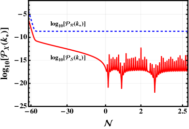
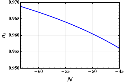
Figure 1: The power spectra of the adiabatic and isocurvature modes and the spectral index $n_{s}$ for the parameter values of BP$a$ in Tab. 1.

In Fig. 1, we show the evolution of power spectra $\mathcal{P}_{\mathcal{R}}$ and $\mathcal{P}_{\mathcal{S}}$ (for the pivot scale $k=k_{*}$) and the spectral index $n_{s}$ for BP$a$. Note, when calculating both power spectra, we solve Eq. (3.31) and Eq. (3.32) numerically without any assumption related to slow-roll. It is clear from Fig. 1 that the isocurvature mode is orders of magnitude smaller than the adiabatic mode and both power spectra freeze out once they exit the horizon. We remark that while finding the power spectrum we always check the orthogonality conditions of Eq. (3.19) in our numerical analysis. In the following, we interchangeably use the cosmological time $t$ and the number of $e$-foldings before the end of inflation which is defined as

$$\mathcal{N}\equiv\ln\frac{a(t)}{a(t_{\rm{end}})}.$$ (3.38)

The pivot scale $k_{*}$ exits the horizon $\mathcal{N_{*}}=$ 57, 59.3, 54.9 $e$-foldings before the end of inflation for BP$a$, BP$b$, and BP$c$, respectively. For illustration, we also show the fields’ time evolution in Fig. 2 for BP$a$, while, the evolution of the Hubble parameter and the inflaton energy density are shown in Fig. 3. It is also clear from Fig. 1 that the spectral index $n_{s}$ lies within the Planck 2018 range when the reference scale exits the horizon. The corresponding values of the tensor-to-scalar ratios are $r_{*}\sim 0.003$, which is consistent with expected values for $R^{2}$-Higgs inflation.

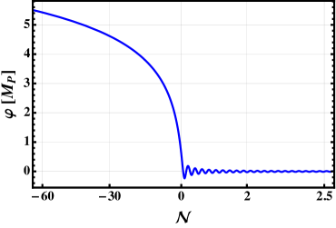
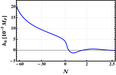
Figure 2: The evolution of the background fields $\varphi$ and the $h_{0}$ for the parameter values of BP$a$ in Tab. 1.

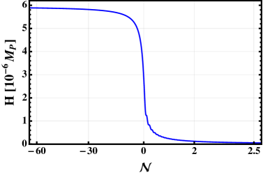
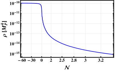
Figure 3: The Hubble function $H$ and the inflaton energy density $\rho$ as in Eq. (3.10a) for the parameter values of BP$a$ given in Tab. 1.

4   Gauge Field Production

The EoM for the gauge field $A_{\mu}$ of Eq. (2.28) can be rewritten as

$$\frac{1}{\sqrt{-g_{E}}}\partial_{\alpha}\left(\sqrt{-g_{E}}g_{E}^{\mu\alpha}g_{E}^{\nu\beta}F_{A\mu\nu}\right)+\frac{8\cos^{2}\theta_{W}M_{\rm P}^{2}}{\xi_{R}\Lambda^{2}}\partial_{\alpha}\left(F(\phi^{I})e^{\sqrt{2/3}\,\phi/M_{\rm P}}\right)\tilde{F}_{A}^{\alpha\beta}$$ (4.1)

$$\hskip 199.16928pt-ieQ_{f}\,e^{-\sqrt{\frac{2}{3}}\frac{\phi}{M_{P}}}g_{E}^{\mu\beta}\bar{f}e^{a}_{\mu}\tilde{\gamma}_{a}f=0,$$

without the presence of a torsion term $F_{A\mu\nu}=D_{\mu}A_{\nu}-D_{\nu}A_{\mu}=\partial_{\mu}A_{\nu}-\partial_{\nu}A_{\mu}$. One can identify the fermion current

$$j^{\mu}=\sum_{f}ieQ_{f}\,e^{-\sqrt{\frac{2}{3}}\frac{\phi}{M_{P}}}g_{E}^{\mu\nu}\bar{f}e^{a}_{\nu}\tilde{\gamma}_{a}f$$ (4.2)

that sources the Schwinger effect.

Neglecting the Schwinger effect

First, we consider the scenario without Schwinger effect i.e. when the fermion current is negligible. This is possible if the fermion field values are small. One can now separate the space and time component of the $A_{\mu}$ field. The time component of Eq. (2.25) at linear order in the perturbations is

$$-\frac{1}{a^{2}}\partial_{i}\left(\partial_{i}A_{0}-\partial_{0}A_{i}\right)=0,$$ (4.3)

which, in temporal gauge $A_{0}=0$, reduces to $\partial_{i}\dot{A}_{i}=0$. The spatial components of Eq. (2.25) are found to be

$$\ddot{A}_{i}+H\dot{A}_{i}-\frac{1}{a^{2}}\partial_{j}\left(\partial_{j}A_{i}-\partial_{i}A_{j}\right)-\frac{\xi H}{a}\epsilon^{ijk}\left(\partial_{j}A_{k}-\partial_{k}A_{j}\right)=0.$$ (4.4)

where

$$H=\frac{\dot{a}}{a},\hskip 56.9055pt\xi=\frac{4\cos^{2}\theta_{W}M_{\rm P}^{2}}{\xi_{R}\Lambda^{2}H}\;\partial_{0}\left(F(\varphi^{I})e^{\sqrt{2/3}\,\varphi/M_{\rm P}}\right).$$ (4.5)

In momentum space, using the notation $\mathbf{A}\equiv\vec{A}$

$$\mathbf{A}(t,\mathbf{x})=\int\frac{d^{3}\mathbf{k}}{\left(2\pi\right)^{3/2}}\tilde{\mathbf{A}}(t,\mathbf{k})e^{-i\mathbf{k}\cdot\mathbf{x}},$$ (4.6)

with $|\mathbf{k}|=k$, Eq. (4.4) reads

$$\ddot{\tilde{\mathbf{A}}}+H\dot{\tilde{\mathbf{A}}}+\frac{k^{2}}{a^{2}}\tilde{\mathbf{A}}+\frac{2i\xi H}{a}(\mathbf{k\times\tilde{A}})=0.$$ (4.7)

The $\tilde{\mathbf{A}}$ field can be written in terms of transverse components as

$$\tilde{\mathbf{A}}=\sum_{\lambda=\pm}\tilde{A}^{\lambda}(t,\mathbf{k})\ \hat{\epsilon}^{\lambda}(\mathbf{k}),~{}\text{with}~{}\mathbf{k}\cdot\hat{\epsilon}^{\lambda}(\mathbf{k})=0,~{}~{}i\mathbf{k}\times\hat{\epsilon}^{\lambda}(\mathbf{k})=\lambda k\ \hat{\epsilon}^{\lambda}(\mathbf{k}).$$ (4.8)

so that, using conformal time $\tau$ (with $\partial_{0}=\partial_{t}={a}^{-1}\partial_{\tau}$), the EoM for the transverse components becomes

$$\partial_{\tau}^{2}\tilde{A}^{\lambda}+\omega_{\lambda}^{2}\tilde{A}^{\lambda}=0,$$ (4.9)

with

$$\omega_{\lambda}^{2}(\tau,k)=k^{2}+2\lambda\xi Hak.$$ (4.10)

In order to quantize the gauge fields, we first integrate Eq. (4.9) by parts to get the action quadratic in the fields

$$S^{\lambda}=\int d\tau\,\mathcal{L}_{\lambda}=\int\,d\tau\,d^{3}\mathbf{k}\,\bigg{[}\frac{1}{2}|\partial_{\tau}\tilde{A}^{\lambda}|^{2}-\frac{1}{2}\omega_{\lambda}^{2}(\tau,k)|\tilde{A}^{\lambda}|^{2}\bigg{]}.$$ (4.11)

As we deal with non-canonical kinetic terms, we apply the quantization procedure detailed in Ref. Lozanov and Amin (2016). The canonical momentum of the transverse modes are

$$\pi_{\lambda}(\tau,\mathbf{k})=\frac{\delta\mathcal{L}_{\lambda}}{\delta\left(\partial_{\tau}\tilde{A}^{\lambda}(\tau,-\mathbf{k})\right)},$$ (4.12)

with the commutation relation expressed as

$$\bigg{[}\tilde{A}^{\lambda}(\tau,\mathbf{k}),\partial_{\tau}\tilde{A}^{\lambda^{\prime}}(\tau,\mathbf{q})\bigg{]}=i\delta_{\lambda\lambda^{\prime}}\delta(\mathbf{k}+\mathbf{q}).$$ (4.13)

The field operator $\tilde{A}^{\lambda}(\tau,\mathbf{k})$ can be written as creation and annihilation operators

$$\tilde{A}^{\lambda}(\tau,\mathbf{k})=\hat{a}_{\mathbf{k}}^{\lambda}u_{k}^{\lambda}(\tau)+\hat{a}_{\mathbf{-k}}^{\lambda}u_{k}^{\lambda\*}(\tau),$$ (4.14)

and the mode equations for the gauge fields are then

$$\ddot{u}^{\lambda}+H\dot{u}^{\lambda}+\frac{\omega_{\lambda}^{2}}{a^{2}}\,u^{\lambda}=0.$$ (4.15)

From these mode functions, we can compute the gauge observables, namely the magnetic and electric fields’ energy densities, magnetic helicity and its derivative, defined as

$$\rho_{B} = \frac{1}{a^{4}}\int_{k_{\text{min}}}^{k_{c}}dk\frac{k^{4}}{4\pi^{2}}\sum_{\lambda}|u^{\lambda}|^{2},$$ (4.16a)

$$\rho_{E} = \frac{1}{a^{4}}\int_{k_{\text{min}}}^{k_{c}}dk\frac{k^{2}}{4\pi^{2}}\sum_{\lambda}|\partial_{\tau}u^{\lambda}|^{2},$$ (4.16b)

$$\mathcal{H} = \frac{1}{a^{3}}\int_{k_{\text{min}}}^{k_{c}}dk\frac{k^{3}}{2\pi^{2}}\left(|u^{+}|^{2}-|u^{-}|^{2}\right),$$ (4.16c)

$$\mathcal{G} = \frac{1}{2}\frac{\partial\mathcal{H}}{\partial t},$$ (4.16d)

with the cut-off value given by Gorbar et al. (2021); Cado and Quirós (2022b)

$$k_{c}=2\left|aH\,\xi\right|,$$ (4.17)

defined by the condition $\omega_{\lambda}^{2}(\tau,k_{c})=0$ satisfied by the helicity $\lambda$ such that $\textrm{sign}(\lambda\xi)=-1$. The corresponding $U(1)_{Y}$ quantities are linked to the electromagnetic ones via

$$\rho_{B_{Y}}=\rho_{B}\;\cos^{2}{\theta_{W}} \rho_{E_{Y}}=\rho_{E}\;\cos^{2}{\theta_{W}}$$ (4.18)

$$\mathcal{H}_{Y}=\mathcal{H}\;\cos^{2}{\theta_{W}} \mathcal{G}_{Y}=\mathcal{G}\;\cos^{2}{\theta_{W}}$$

In general, the integration limits should cover all modes from zero to infinity, however, not all modes are amplified during inflation. At the time $t$, the cut-off mode $k_{c}$ is found by the solution of $\omega_{\lambda}=0$; essentially this is when a mode $k=k_{c}$ crosses the horizon for the first time (at least for one helicity). The modes $k\gg k_{c}$ are not excited during inflation and can be neglected for the estimation of the above observable quantities. We will discuss $k_{\rm{min}}$ shortly.

In order to find $\rho_{B}$, $\rho_{E}$, $\mathcal{H}^{\rm{num}}$ and $\mathcal{G}^{\rm{num}}$ we solve Eq. (4.15) numerically via fourth-order Runge-Kutta (RK4) method in discrete time steps. We outline the details in Appendix E. For the $i$-th time step, the gauge field modes are initialized with the Bunch-Davies (BD) initial condition as Cuissa and Figueroa (2019)

$$u_{\lambda}(k,t_{i})\simeq\frac{1}{\sqrt{2k}}e^{-i\omega_{i}t_{i}},\hskip 71.13188pt\dot{u}_{\lambda}\simeq-i\frac{\omega_{i}}{\sqrt{2k}}e^{-i\omega_{i}t_{i}},$$ (4.19)

with $\omega_{i}={k}{a^{-1}(t_{i})}$. It is practically not possible to go to the infinite past. Hence, to ensure that all modes remain well within the horizon at the initial time step $t_{\rm{in}}$, we chose $k_{\rm{min}}=x_{\rm{BD}}a(t_{\rm{in}})H(t_{\rm{in}})$ with $x_{\rm{BD}}=100$. On the one hand, if a mode $k$ remains well within the horizon, $k>x_{\rm{BD}}\,a(t_{i})H(t_{i})$, we directly assume the BD solutions for the modes instead of applying the RK4 method for any subsequent time step. On the other hand, all superhorizon modes are solved with the RK4 method. For the numerical solution discussed below, we employ 25k time steps.

In Fig. 4, we show the evolution of $\rho_{B}$, $\rho_{E}$, $\mathcal{H}^{\rm{num}}$ and $\mathcal{G}^{\rm{num}}$ for BP$a$ with $\Lambda=2.55\times 10^{-5}M_{\rm P}$ for illustration. Similar values are found for the other benchmark points. We remark that we have compared our numerical results to the analytical approximation of the magnetic and electric fields’ energy densities, magnetic helicity, and its derivative as in Ref. Cado and Quirós (2022b) and find good agreement.

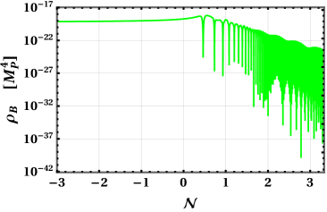
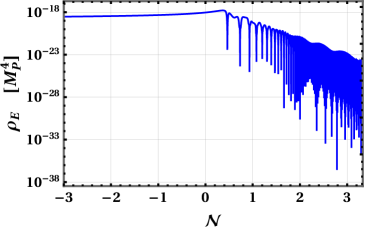
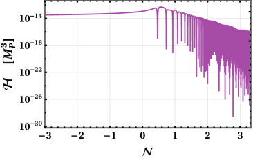
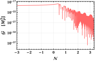
Figure 4: In the upper panel we plot the energy densities $\rho_{B}$ and $\rho_{E}$ with $\Lambda=2.55\times 10^{-5}$ $M_{\rm P}$ for the BP$a$ summarized in Tab. 1. The lower panel corresponds to the hyperhelical magnetic fields $\mathcal{H}$ and $\mathcal{G}$ for identical parameter choices.

Relevance of the Schwinger effect

We now turn to the impact of the Schwinger effect. The fermion current of Eq. (4.2) can be expressed as

$$j^{\mu}=(\rho_{\rm c},\bm{J})$$ (4.20)

The current and the gauge field are related by Ohm’s law

$$\bm{J}=\sigma_{\rm c}\,\bm{E}=-\sigma_{\rm c}\,\partial_{\tau}\bm{A},$$ (4.21)

where the conductivity $\sigma_{\rm c}$ has been defined as a comoving quantity. The physical conductivity $\sigma_{\rm ph}$ relates to the comoving one via $\sigma_{\rm c}=a\,\sigma_{\rm ph}$. In the case of one Dirac fermion $f$ with mass $m_{f}$ and charge $Q_{f}$ under a $U(1)$ group with coupling $g$, the comoving conductivity associated to $f$ can be written as Domcke and Mukaida (2018)

$$\sigma_{f}^{\rm c}=\frac{|g\,Q_{f}|^{3}}{6\pi^{2}}\frac{a}{H}\;\sqrt{2\rho_{B}}\;\coth\left(\pi\sqrt{\frac{\rho_{B}}{\rho_{E}}}\right)\exp{-\frac{\pi m_{f}^{2}}{\sqrt{2\rho_{E}}\,|g\,Q_{f}|}-\sqrt{\frac{2}{3}}\frac{\phi}{M_{P}}},$$ (4.22)

where $m_{f}\equiv m_{f}(h_{0})=m_{f}(v)h_{0}/v$ and so that

$$\sigma_{\rm c}=\sum_{f}\sigma^{\rm c}_{f}=\sum_{\ell}\sigma^{\rm c}_{\ell}+N_{c}\sum_{q}\sigma^{c}_{q},$$ (4.23)

with $\ell=e,\mu,\tau$; $q=u,d,c,s,t,b$, $N_{c}=3$ being the number of colors. Last, since we are in the broken phase, we identify $g$ as the electric charge $g\equiv e\simeq 0.71$ at the scale in which inflation takes place.

This conductivity is to be distinguished from the conductivity of a thermal plasma after reheating in a radiation-dominated universe. We stress that the above is the conductivity at the end of inflation, before the reheating, produced by fermion pair formation from the magnetic field. Also, this estimation is valid in the case of collinear electric and magnetic fields, an assumption that we have numerically checked. Finally, the electric and magnetic fields are assumed to be slowly varying, as we expect the hypercharge gauge field to reach a stationary configuration, where the tachyonic instability and the induced current balance each other. We have verified in our numerical simulation that this is indeed the case.

In the presence of the fermion current, Eq. (4.7) becomes

$$\ddot{\tilde{\mathbf{A}}}+(H+\sigma_{\rm ph})\,\dot{\tilde{\mathbf{A}}}+\frac{k^{2}}{a^{2}}\;\tilde{\mathbf{A}}+\frac{2iH\xi}{a}\;(\mathbf{k\times\tilde{A}})=0,$$ (4.24)

which, for the transverse components in conformal time reads as

$$\partial_{\tau}^{2}\tilde{A}^{\lambda}+\sigma_{\rm c}\,\partial_{\tau}\tilde{A}^{\lambda}+\omega_{\lambda}^{2}\tilde{A}^{\lambda}=0,$$ (4.25)

which can be recast as

$$\partial_{\tau}^{2}\tilde{A}^{\lambda}+\left(\frac{\partial}{\partial\tau}\log(\Delta(\tau))\right)\partial_{\tau}\tilde{A}^{\lambda}+\omega_{\lambda}^{2}\tilde{A}^{\lambda}=0,$$ (4.26)

with

$$\Delta(\tau)=\exp{\int_{-\infty}^{\tau}\sigma_{\rm c}(\tau^{\prime})\,d\tau^{\prime}}.$$ (4.27)

Integrating Eq. (4.26) by parts as in the previous subsection, one can now define the canonical momentum for the transverse modes as

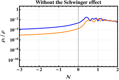
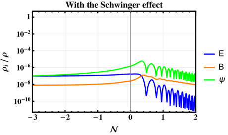
Figure 5: Energy breakdown for $\xi_{R}=2.35\times 10^{9}$, $\xi_{H}=10^{-3}$ and $\Lambda=2\times 10^{-5}M_{\rm P}$ at the end of inflation and the onset of reheating. We show a comparison between the absence and the presence of the Schwinger effect for the quantities $\rho_{i}(\mathcal{N})/\rho(\mathcal{N})$, $i=E,B,\psi$. When the Schwinger effect is strong, like here, the fermion energy density can dominate over the gauge density. Still, all energy shares are reduced in the presence of the Schwinger effect.

$$\pi_{\lambda}(\tau,\mathbf{k})=\frac{\delta\mathcal{L}_{\lambda}}{\delta\left(\partial_{\tau}\tilde{A}^{\lambda}(\tau,-\mathbf{k})\right)}=\Delta(\tau)\partial_{\tau}\tilde{A}^{\lambda^{\prime}}(\tau,\mathbf{k}),$$ (4.28)

and the commutation relation now becomes Lozanov and Amin (2016)

$$\bigg{[}\tilde{A}^{\lambda}(\tau,\mathbf{k}),\partial_{\tau}\tilde{A}^{\lambda^{\prime}}(\tau,\mathbf{q})\bigg{]}=i\frac{1}{\Delta(\tau)}\delta_{\lambda\lambda^{\prime}}\delta(\mathbf{k}+\mathbf{q}),~{}~{}\mbox{with,}~{}\tilde{A}^{\lambda}(\tau,\mathbf{k})=\hat{a}_{\mathbf{k}}^{\lambda}u_{k}^{\lambda}(\tau)+\hat{a}_{\mathbf{-k}}^{\lambda}u_{k}^{\lambda\*}(\tau).$$ (4.29)

The mode equations for the gauge fields in the presence of the Schwinger effect become

$$\ddot{u}^{\lambda}+(H+\sigma_{\rm c})\dot{u}^{\lambda}+\frac{k}{a}\bigg{(}\frac{k}{a}+2\lambda H\xi\bigg{)}u^{\lambda}=0,$$ (4.30)

and the cut-off momenta $k_{c}$ is now modified to

$$k_{c}=\left|aH\,\xi\right|+\sqrt{\left(aH\,\xi\right)^{2}+\frac{a^{2}}{2}\left[\dot{\sigma}_{\rm ph}+\sigma_{\rm ph}\left(\frac{\sigma_{\rm ph}}{2}+H\right)\right]}\,.$$ (4.31)

At early times solution of the mode equations of Eq. (4.30) are represented by WKB solution Lozanov and Amin (2016); Sfakianakis and van de Vis (2019)

$$u^{\lambda}(\tau)=\frac{1}{\sqrt{2}}\frac{1}{\sqrt{\Delta(\tau)\omega_{\lambda}(\tau,k)}}\;e^{-i\int_{\tau_{\rm{in}}}^{\tau}d\tau^{\prime}\omega_{\lambda}(\tau^{\prime},k)}$$ (4.32)

as long as $|\frac{\partial_{\tau}\omega_{\lambda}}{\omega_{\lambda}}|\ll 1$. In practice, we utilize the early-time solution for the modes

$$u^{\lambda}(\tau)=\frac{1}{\sqrt{2}}\frac{1}{\sqrt{\Delta(\tau)\omega_{\lambda}(\tau,k)}}\;e^{-ik\tau}$$ (4.33)

to find relevant, observable quantities. From Eq. (4.30) and Eq. (4.31), we find the energy densities for BP$a$ and display them in the right panel of Fig. 5.

Due to the coupling between the fermion and gauge sectors, massless hypercharged fermions are continuously produced during inflation. They are massless as long as the EW symmetry remains intact and thus contribute to the energy density of relativistic radiation as

$$\rho_{\psi}=\lim_{V\to\infty}\dfrac{\sigma}{V}\int_{V}d^{3}x\;\frac{\langle\bm{A}\cdot\bm{E}\rangle}{a^{4}}=\frac{\sigma}{a^{4}}\int^{k_{c}}_{k_{\rm min}}dk\,\frac{k^{2}}{2\pi^{2}}\dfrac{d}{d\tau}\sum_{\lambda}|u^{\lambda}|^{2}.$$ (4.34)

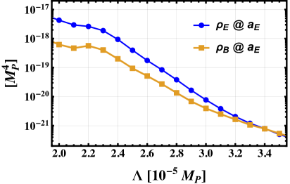
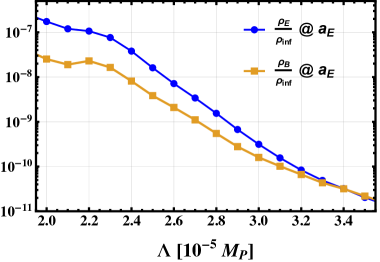
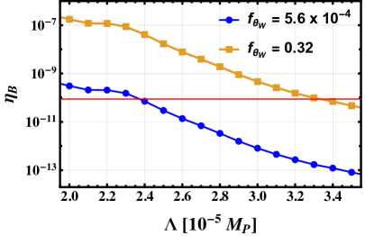
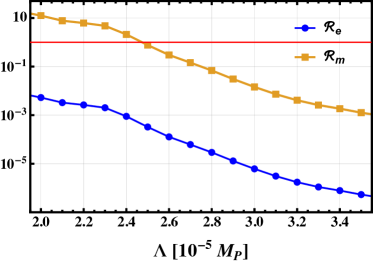
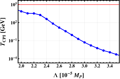
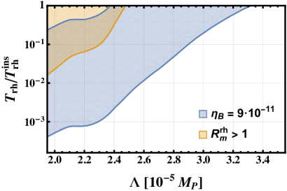
Figure 7: Similar to Fig. 6, these figures again display a scan of the parameter $\Lambda$ with the first set of initial conditions, BP$a$ in Tab. 1 including the Schwinger effect. Top panels: Magnetic and electric energy density (left) and their ratio with the inflation energy density (right). Middle panel: baryon asymmetry $\eta_{B}$ (left) and Reynolds numbers (right) with their corresponding constraints in red. Bottom panels: CPI temperature with constraint in red (left) and baryogenesis parameter space (right). We did not display the CPI temperature on this last plot as the CPI is no longer a constraint.

It has been shown in Ref. Gorbar et al. (2021) that the fermion energy density can easily dominate over the energy densities of $E$ and $B$ fields at the end of inflation. This situation has been chosen as an example in Fig. 5 where we display the energy fraction $\rho_{i}(\mathcal{N})/\rho(\mathcal{N})$, $i=E,B,\psi$ at the end of inflation and the onset of reheating. We show a direct comparison between the presence and the absence of the Schwinger effect. While for $\Lambda\gtrsim 4\times 10^{-5}M_{P}$ the difference is an order one factor, the Schwinger effect reduces the amount of electromagnetic energy and helicity up to two orders of magnitude for $\Lambda\simeq 2.4\times 10^{-5}M_{P}$, see Fig. 7. This is because the presence of the Schwinger effect trades an exponential behaviour in $\xi$ with a polynomial one.

When the gauge share dominates at least by 80%, the Universe will reheat before the perturbative decay of the inflaton Cuissa and Figueroa (2019), a phenomenon called gauge preheating. As in Ref. Cado and Quirós (2022b), we found that preheating is unlikely since the ratio is $\sim 10^{-6}$ at most. However, the huge damping in both energy and helicity does not preclude a window in the parameter space where the BAU is achieved, as we will see in the next section.

5   Baryogenesis

To generate a baryon asymmetry, the Sakharov conditions Sakharov (1967) must be met: (i) the system must contain a process that violates the baryon number, (ii), this process also violates C/CP symmetries, (iii) this process occurs out of thermal equilibrium. In the SM, the CP-violating term from the CKM matrix phase is too small to induce a significant baryon asymmetry at a low energy scale, hence we included the dimension-six CP-odd term between Ricci scalar and $U(1)_{Y}$ gauge boson. On the other hand, in the symmetric phase of the EW plasma, the SM exhibits a chiral anomaly that is enough to source the present-day BAU. The anomaly expresses the fact that the $B+L$ anomaly, the $U(1)_{Y}$ helicity and the weak sphaleron are connected as

$$\Delta N_{B}=\Delta N_{L}=N_{g}\left(\Delta N_{\rm CS}-\dfrac{g^{\prime 2}}{16\pi^{2}}\;\Delta\mathcal{H}_{Y}\right).$$ (5.1)

The factor $N_{g}=3$ is the number of fermion generations and $g^{\prime}$ is the $U(1)_{Y}$ gauge coupling. Under the thermal fluctuation of the $SU(2)_{L}$ gauge fields, the Chern-Simons number $N_{\rm CS}$ is diffusive, resulting in the rapid washout of both lepton $N_{L}$ and baryon $N_{B}$ numbers. On the contrary, a helical primordial magnetic field acts as a source, and a net baryon asymmetry can remain after the EW phase transition.

In Refs. Kamada and Long (2016a, b), the effects of the helicity decay and sphaleron washout balance have been studied within a careful analysis of the transport equations for all SM species during the EWPT. As a result, a non-zero baryon-to-entropy ratio $\eta_{B}$ remains in the broken phase while the transformation of baryon asymmetry back into helicity is avoided. The novelty of the mechanism lies in the introduction of a time-dependent (temperature-dependent) weak mixing angle $\theta_{W}(T)$ which enters an additional source of the baryon number into the kinetic equation. When the EW symmetry breaking occurs at $T\simeq 160$ GeV, the primordial hypermagnetic field becomes an electromagnetic field. However, the electroweak sphaleron remains in equilibrium until $T\simeq 130$ GeV and threatens to washout the baryon asymmetry. Therefore proper modeling of the epoch 160 GeV $\gtrsim T\gtrsim 130$ GeV is critical to an accurate prediction of the relic BAU.

The behavior of $\theta_{W}(T)$ is confirmed by analytic calculations Kajantie et al. (1997), and numerical lattice simulations D’Onofrio and Rummukainen (2016). We follow Refs. Kamada and Long (2016b); Jiménez et al. (2017) and model it with a smooth step function

$$\cos^{2}\theta_{W}=\frac{g^{2}}{g^{\prime 2}+g^{2}}+\frac{1}{2}\frac{g^{\prime 2}}{g^{\prime 2}+g^{2}}\left(1+\tanh\left[\frac{T-T_{\rm step}}{\Delta T}\right]\right)$$ (5.2)

which, for $155\,\text{GeV}\lesssim T_{\rm step}\lesssim 160\,\text{GeV}$ and $5\,\text{GeV}\lesssim\Delta T\lesssim 20\,\text{GeV}$, describes reasonably well the analytical and lattice results for the temperature dependence. Consequently, it is possible to generate the observed BAU from a maximally helical magnetic field that was generated before the EW crossover. Indeed, including all contributions, the Boltzmann equation for the baryon-to-entropy ratio $\eta_{B}$ reads

$$\frac{d\eta_{B}}{dx}\,=\,-\frac{111}{34}\gamma_{W\rm sph}\,\eta_{B}\,+\,\frac{3}{16\pi^{2}}(g^{\prime 2}+g^{2})\sin(2\theta_{W})\frac{d\theta_{W}}{dx}\,\frac{\mathcal{H}_{Y}}{s},$$ (5.3)

where $x=T/H(T)$, with $H(T)$ being the Hubble rate at temperature $T$, $\mathcal{H}_{Y}$ the hypermagnetic helicity that is initially present and $s$ the comoving entropy density of the SM plasma given by $s=(2\pi^{2}/45)g_{\ast}T^{3}$. Furthermore, $\gamma_{W\rm sph}=6\,\Gamma_{W\rm sph}/T^{4}$ is the dimensionless transport coefficient for the EW sphaleron which, for temperatures $T<161$ GeV, is found from lattice simulations to be D’Onofrio et al. (2014)

$$\gamma_{W\rm sph}\,\simeq\,\exp{-147.7+107.9\;\frac{T}{130\,\text{GeV}}}.$$ (5.4)

The Boltzmann equation (5.3) has been numerically solved in Ref. Kamada and Long (2016b) and the baryon-to-entropy ratio $\eta_{B}$ was found to become frozen, i.e. $\dot{\eta}_{B}=0$, at a temperature $T\simeq 135$ GeV. As expected, this is close to the temperature $T\simeq 130$ GeV at which EW sphalerons freeze out. Setting the RHS of Eq. (5.3) to zero and solving for $\eta_{B}$ yields

$$\eta_{B}\simeq 4\cdot 10^{-12}\,f_{\theta_{W}}\frac{\mathcal{H}_{Y}}{H^{3}(t_{\text{end}})}\left(\frac{H(t_{\text{end}})}{10^{13}\,\text{GeV}}\right)^{\frac{3}{2}}\left(\frac{T_{\rm rh}}{T_{\rm rh}^{\rm ins}}\right),$$ (5.5)

where the (instant) reheating temperature is

$$T_{\rm rh}=\left(\frac{90}{\pi^{2}g_{\ast}}\right)^{\frac{1}{4}}\sqrt{\Gamma_{\phi}},\hskip 42.67912ptT_{\rm rh}^{\rm ins}=\left(\frac{90}{\pi^{2}g_{\ast}}\right)^{\frac{1}{4}}\sqrt{H(t_{\text{end}})},$$ (5.6)

and $\Gamma_{\phi}$ is the total decay width of the inflaton that reheats the universe after inflation.

All the details on the EWPT dynamics are encoded in the parameter $f_{\theta_{W}}$ which is subject to significant uncertainties

$$f_{\theta_{W}}=-\sin(2\theta_{W})\,\dfrac{d\theta_{W}}{d\log T}\bigg{\rvert}_{T=135\text{ GeV}},\hskip 42.67912pt5.6\cdot 10^{-4}\lesssim f_{\theta_{W}}\lesssim 0.32.$$ (5.7)

The bounds on $f_{\theta_{W}}$ are given by varying $T_{\rm step}$ and $\Delta T$ in the ranges given below Eq. (5.2). The result Eq. (5.5) is a main ingredient of this work as it directly relates the amount of the final BAU to the amount of hypermagnetic helicity available at the EWPT.

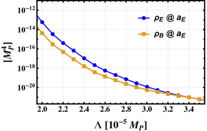
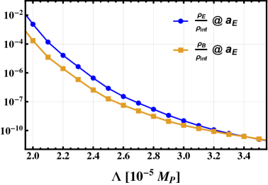
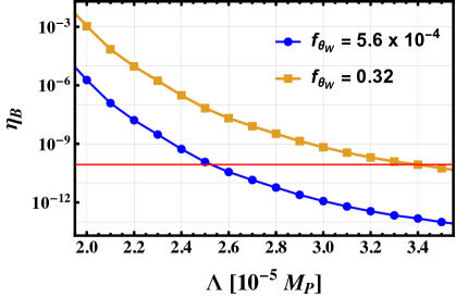
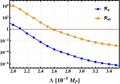
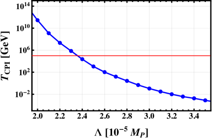
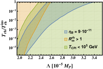
Figure 6: These figures display a scan of the parameter $\Lambda$ with the first set of initial conditions, see BP$a$ in Tab. 1 without Schwinger effect. Top panels: Magnetic and electric energy density (left) and their ratio with the inflation energy density (right). Middle panel: baryon asymmetry $\eta_{B}$ (left) and Reynolds numbers (right) with their corresponding constraints in red. Bottom panels: CPI temperature with constraint in red (left) and baryogenesis parameter space (right).

The production of hypermagnetic fields nevertheless happens at the inflationary scale, hence one must ensure that the helicity is preserved as the Universe cools down in the radiation-dominated era that follows reheating. A rough estimate is to require that the magnetic Reynolds number $\mathcal{R}_{m}$ is bigger than unity, as this implies that the effects of magnetic induction are dominating over magnetic diffusion in the thermal plasma. On the other hand, the electric Reynolds number $\mathcal{R}_{e}$ determines in which regime the plasma evolves and informs us how to calculate the magnetic Reynolds number, see e.g. Refs. Domcke et al. (2019); Cado and Quirós (2022a). In our work, we found that we are in the viscous regime, $\mathcal{R}_{e}<1$, and hence we need to satisfy the constraint

$$\mathcal{R}_{m}^{\rm rh}\approx 5.9\cdot 10^{-6}\;\frac{\rho_{B_{Y}}\ell_{B_{Y}}^{2}}{H(t_{\text{end}})^{2}}\left(\frac{H(t_{\text{end}})}{10^{13}\,\text{GeV}}\right)\left(\frac{T_{\rm rh}}{T_{\rm rh}^{\rm ins}}\right)^{\frac{2}{3}}>1,$$ (5.8)

where $\ell_{B_{Y}}$ is the hypermagnetic characteristic size given by

$$\ell_{B_{Y}}=\frac{2\pi}{\rho_{B}\,a^{3}}\int_{k_{\text{min}}}^{k_{c}}dk\,\frac{k^{3}}{4\pi^{2}}\sum_{\lambda}|u^{\lambda}|^{2}.$$ (5.9)

The magnetohydrodynamics description of the plasma also admits a CP-odd term that can induce a helicity cancellation because of the fermion asymmetry back-transformation into helical gauge fields with opposite sign. This is because the energy configuration in the gauge sector is more favorable than in the fermion sector Joyce and Shaposhnikov (1997), a phenomenon called chiral plasma instability (CPI). Thus, one must ensure that all fermion asymmetry created alongside the helical field during inflation is erased by the action of the weak sphaleron for $10^{12}\text{ GeV}\gtrsim T\gtrsim 130$ GeV. Because the weak interaction only couples to left-handed fermions, the right-handed fermions are protected from the washout until their Yukawa interaction becomes relevant in thermal equilibrium. The right-handed electron $e_{R}$ is the last species to come into chemical equilibrium, at temperatures $\sim 10^{5}\,$GeV, thus its asymmetry survives the longest. Therefore, to efficiently erase the fermion asymmetry, while preserving the helicity in the gauge sector, before the CPI can happen, one must require that Joyce and Shaposhnikov (1997); Domcke et al. (2019)

$$T_{\rm CPI}\approx(4\cdot 10^{-7}\;\text{GeV})\,\;\frac{\mathcal{H}_{Y}^{2}}{H(t_{\text{end}})^{6}}\,\left(\frac{H(t_{\text{end}})}{10^{13}\,\text{GeV}}\right)^{3}\left(\frac{T_{\rm rh}}{T_{\rm rh}^{\rm ins}}\right)^{2}\lesssim 10^{5}\text{ GeV}.$$ (5.10)

In Figs. 6 and 7, we display the main results for the baryogenesis mechanism both in the presence and absence of the Schwinger effect. In both figures, the top panels display the electromagnetic energy and energy ratio to the background energy density. In the middle panels we show the quantities $\eta_{B}(\Lambda,f_{\theta_{W}})$, $\mathcal{R}_{m}(\Lambda)$ and $\mathcal{R}_{e}(\Lambda)$. On the left, the red line must be in between the two curves to meet the constraint. On the right, the only constraint is that $\mathcal{R}_{m}$ is above the red line. Finally, at the bottom, we present the CPI temperature as a function of $\Lambda$ and the regions where the different constraints are met. On the bottom left panel, the curve should be below the red line. On the right one, we shall seek the overlapping region. In this last plot, we add the temperature ratio $T_{\rm rh}\,/\,T_{\rm rh}^{\rm ins}$ as a supplementary parameter. We see that the window is larger in the presence of the Schwinger, which also totally removes the constraint on $T_{\rm CPI}$. Indeed, the backreactionless mechanism tends to overshoot the BAU, an issue addressed by the presence of the Schwinger effect which therefore acts as a BAU facilitator.

6   Summary and Conclusions

We have discussed baryogenesis in the context of $R^{2}$-Higgs inflation, involving the CP-violating dimension-six term proportional to $(R/\Lambda^{2})\,B_{\mu\nu}\tilde{B}^{\mu\nu}$. We adopt a fully covariant formalism for both inflationary dynamics and gauge field production. Our linear order analysis shows that if $\Lambda\sim 3\times 10^{-5}M_{\rm P}$, sufficient helical hypermagnetic fields are produced, which can lead to the observed BAU during the electroweak crossover. Smaller values of $\Lambda$ imply an overproduction of baryons. Once the Schwinger effect is included, the energy densities $\rho_{E}$ and $\rho_{B}$ are suppressed, but there is a subtlety: the Schwinger effect is exponentially suppressed by a factor $\sim\exp(-\sqrt{(2/3)}\,{\varphi}/{M_{P}})$, which dilutes its relevance during the inflationary epoch, but becomes pronounced around and after the end of inflation. The Schwinger effect can then lead to baryogenesis for smaller values $\Lambda\sim 2.2\times 10^{-5}M_{\rm{P}}$. We also find that when the Schwinger effect is included, the radiation density $\rho_{\psi}$ can dominate over the electromagnetic densities $\rho_{E}$ and $\rho_{B}$, cf. Fig. 5.

We have primarily focused on the Starobinsky-like regime in our linear order analysis. In the mixed $R^{2}$-Higgs scenario, a smaller $\Lambda$ may generate BAU without the Schwinger effect. This can be understood from Eq. (2.25) where a smaller $\xi_{R}$ and moderately large $\xi_{H}$ (i.e. the mixed $R^{2}$-Higgs like regime) can induce inflation, while BAU is triggered by a smaller scale $\Lambda$ without relying on the Schwinger effect. However, a larger $\xi_{H}$ may lead to an exponential growth of isocurvature modes (see e.g. Refs. Bassett et al. (2000); Liddle et al. (2000); Gordon et al. (2000)) in our backreactionless scenario although such a mode is suppressed during inflation. Moreover, in such a scenario, one would need to take into account non-perturbative effects. In our analysis, we have not considered the impact of decay and self-resonance. Thus, the ratio $T_{\rm rh}/T_{\rm rh}^{\rm ins}$ is essentially a free parameter in our analysis. We leave a more detailed analysis of (p)reheating and particle production for future work. It has been pointed out that the helical gauge fields may source non-gaussianity Barnaby and Peloso (2011); Barnaby et al. (2012), which may result in moderate constraint to the parameter space for baryogenesis without the Schwinger effect Cado and Quirós (2022a). In the presence of the Schwinger effect, the produced helical gauge fields are much weaker and we expect those constraints to be harmless. However, one needs to be careful when interpreting results from Refs. Barnaby and Peloso (2011); Barnaby et al. (2012) as they focus on a single field. In our multi-field model, a proper estimation of non-gaussianity requires considering perturbations up to third order. This would induce several new contributions from field-space Riemann tensor Kaiser et al. (2013) and is beyond the scope of our work.

While there are many avenues to achieve the observed BAU, baryogenesis driven by a dimension-six CP-odd term $\sim(R/\Lambda^{2})\,B_{\mu\nu}\tilde{B}^{\mu\nu}$ provides a motivated approach to address BAU within the framework of $R^{2}$-Higgs inflation. This approach critically rests on the presence of an effective dimension-six term, but it does not require additional degrees of freedom beyond the SM. In parallel, such dimension-six terms can also shed light on the UV sensitivity of $R^{2}$-Higgs inflation as discussed in, e.g. Refs. Modak et al. (2023); Lee et al. (2023).

Acknowledgments — YC acknowledges funding support from the Initiative Physique des Infinis (IPI), a research training program of the Idex SUPER at Sorbonne Université. CE is supported by the UK Science and Technology Facilities Council (STFC) under grant ST/X000605/1 and the Leverhulme Trust under RPG-2021-031. TM is funded by the Deutsche Forschungsgemeinschaft (DFG, German Research Foundation) under grant 396021762 — TRR 257: Particle Physics Phenomenology after the Higgs Discovery and Germany’s Excellence Strategy EXC 2181/1 — 390900948 (the Heidelberg STRUCTURES Excellence Cluster). The work of MQ is partly supported by Spanish MICIN under Grant PID2020-115845GB-I00, and by the Catalan Government under Grant 2021SGR00649. IFAE is partially funded by the CERCA program of the Generalitat de Catalunya.

Appendix A The Vierbein Fields

The vierbein fields $e^{a}_{\mu}$ are defined as follows: The metric in the Jordan frame $g_{J\mu\nu}$ can be related at every point to a Minkowski tangent space $\eta_{ab}$ via the vierbein, which obeys the following orthogonality conditions

$$e_{\mu}^{a}e_{a}^{\nu}=\delta^{\nu}_{\mu},~{}~{}e_{\mu}^{a}e_{b}^{\mu}=\delta^{a}_{b},~{}~{}g_{J\mu\nu}=e_{\mu}^{a}e_{\nu}^{b}\eta_{ab}~{}\mbox{and}~{}\gamma_{\mu}=e^{a}_{\mu}\tilde{\gamma}_{a},$$ (A.1)

where $\tilde{\gamma}_{a}$ are the Minkowski $\gamma$-matrices. The $\gamma_{\mu}$ satisfy $\{\gamma^{\mu},\gamma^{\nu}\}=2g_{J}^{\mu\nu}$ in curved space-time. The spin-affine connection is given by

$$\Gamma_{\mu}=\frac{1}{2}\omega_{\mu\;ab}\sigma^{ab}~{}\text{with}~{}\sigma^{ab}=\frac{1}{4}[\tilde{\gamma}^{a},\tilde{\gamma}^{b}].$$ (A.2)

The spin-connection $\omega^{\;a}_{\mu\;\;b}$ is defined as Collas and Klein (2019)

$$\omega^{\;a}_{\mu\;\;b}\equiv\left(e_{\nu}^{a}e^{\beta}_{b}\Gamma^{\nu}_{\mu\beta}-e^{\beta}_{b}\partial_{\mu}e_{\beta}^{a}\right).$$ (A.3)

Appendix B Field-Space Metric and Christoffel Symbols

The field-space $G^{IJ}$ metric is given by

$$G^{\phi\phi}=1,~{}~{}G^{hh}=e^{\sqrt{\frac{2}{3}}\frac{\phi}{M_{\rm P}}},~{}~{}G^{\phi h}=G^{h\phi}=0.$$ (B.1)

The corresponding non-vanishing Christoffel symbols are therefore

$$\Gamma^{\phi}_{hh}=\frac{e^{-\sqrt{\frac{2}{3}}\frac{\phi}{M_{\rm P}}}}{\sqrt{6}M_{\rm P}},~{}~{}\Gamma^{h}_{\phi h}=\Gamma^{h}_{h\phi}=-\frac{1}{\sqrt{6}M_{\rm P}}.$$ (B.2)

Appendix C Einstein Equation and Stress-Energy Tensor

The action $S_{E}$ can be rewritten in the following way

$$S_{E} =\int d^{4}x\sqrt{-g_{E}}\bigg{(}\frac{M_{\rm P}^{2}}{2}R_{E}+\mathcal{L}_{M}\bigg{)},$$ (C.1)

where $\mathcal{L}_{M}$ is all terms in the action other than $R_{E}$. Varying the action with respect to $g_{E}^{\mu\nu}$ we get

$$0 =\delta S_{E}$$

$$=\int d^{4}x\left(\frac{M_{\rm P}^{2}}{2}\frac{\delta(\sqrt{-g_{E}}R_{E})}{\delta g_{E}^{\mu\nu}}+\frac{\delta(\sqrt{-g_{E}}\mathcal{L}_{M})}{\delta g_{E}^{\mu\nu}}\right)\delta g_{E}^{\mu\nu}$$ (C.2)

$$=\int d^{4}x\left(\frac{M_{\rm P}^{2}}{2}\left(R_{E}\frac{\delta(\sqrt{-g_{E}})}{\delta g_{E}^{\mu\nu}}+\sqrt{-g_{E}}\frac{\delta(R_{E})}{\delta g_{E}^{\mu\nu}}\right)+\sqrt{-g_{E}}\frac{\delta(\mathcal{L}_{M})}{\delta g_{E}^{\mu\nu}}+\mathcal{L}_{M}\frac{\delta(\sqrt{-g_{E}})}{\delta g_{E}^{\mu\nu}}\right)\delta g_{E}^{\mu\nu}.$$

Utilizing $\frac{\delta(\sqrt{-g_{E}})}{\delta g_{E}^{\mu\nu}}=-\frac{1}{2}\sqrt{-g_{E}}g_{E\mu\nu}$, $\frac{\delta(R_{E})}{\delta g_{E}^{\mu\nu}}=R_{E\mu\nu}$ and ignoring the surface term we get

$$R_{E\mu\nu}-\frac{1}{2}g_{E\mu\nu}R_{E} =\frac{1}{M_{\rm P}^{2}}T_{\mu\nu}$$ (C.3)

where

$$T_{\mu\nu}=\left(\mathcal{L}_{M}g_{E\mu\nu}-2\frac{\delta\mathcal{L}_{M}}{\delta g_{E}^{\mu\nu}}\right),$$ (C.4)

which is found to be

$$\begin{split}T_{\mu\nu}&=\bigg{[}G_{IJ}D_{\mu}\phi^{I}D_{\nu}\phi^{J}+g_{E}^{\alpha\beta}B_{\alpha\mu}B_{\beta\nu}+g_{E}^{\alpha\beta}W^{i}_{\alpha\mu}W^{i}_{\beta\nu}+\frac{1}{2}e^{-\sqrt{\frac{2}{3}}\frac{\phi}{M_{\rm P}}}g^{2}h^{2}\frac{(W^{1}_{\mu}-iW^{2}_{\mu})}{\sqrt{2}}\frac{(W^{1}_{\nu}+iW^{2}_{\nu})}{\sqrt{2}}\\ &+\frac{2cM_{\rm P}^{2}}{\xi_{R}\Lambda^{2}\sqrt{-g_{E}}}F(\phi^{I})e^{\sqrt{2/3}\,\phi/M_{\rm P}}\left(2g_{E\mu\alpha}\epsilon^{\alpha\beta\rho\sigma}B_{\nu\beta}B_{\rho\sigma}+\frac{1}{8}g_{E\mu\nu}\epsilon^{\alpha\beta\rho\sigma}B_{\alpha\beta}B_{\rho\sigma}\right)\\ &+\frac{1}{4}e^{-\sqrt{\frac{2}{3}}\frac{\phi}{M_{\rm P}}}h^{2}\left(gW^{3}_{\mu}-g^{\prime}B_{\mu}\right)\left(gW^{3}_{\nu}-g^{\prime}B_{\nu}\right)\bigg{]}-\\ &g_{E\mu\nu}\bigg{(}\frac{1}{2}G_{IJ}g_{E}^{\alpha\beta}D_{\alpha}\phi^{I}D_{\beta}\phi^{J}+V_{0}(\phi^{I})+\frac{2cM_{\rm P}^{2}}{\xi_{R}\Lambda^{2}\sqrt{-g_{E}}}F(\phi^{I})e^{\sqrt{2/3}\,\phi/M_{\rm P}}B_{\alpha\beta}\tilde{B}^{\alpha\beta}\\ &+\dfrac{1}{4}g_{E}^{\alpha\rho}g_{E}^{\beta\sigma}B_{\alpha\beta}B_{\rho\sigma}+\dfrac{1}{4}g_{E}^{\alpha\rho}g_{E}^{\beta\sigma}W^{i}_{\alpha\beta}W^{i}_{\rho\sigma}+\frac{1}{4}e^{-\sqrt{\frac{2}{3}}\frac{\phi}{M_{\rm P}}}g_{E}^{\alpha\beta}g^{2}h^{2}\frac{(W^{1}_{\alpha}-iW^{2}_{\alpha})}{\sqrt{2}}\frac{(W^{1}_{\beta}+iW^{2}_{\beta})}{\sqrt{2}}\\ &+\frac{1}{8}e^{-\sqrt{\frac{2}{3}}\frac{\phi}{M_{\rm P}}}g_{E}^{\alpha\beta}h^{2}\left(gW^{3}_{\alpha}-g^{\prime}B_{\alpha}\right)\left(gW^{3}_{\beta}-g^{\prime}B_{\beta}\right)\bigg{)}+e^{-\sqrt{\frac{2}{3}}\frac{\phi}{M_{\rm P}}}\bar{f}e^{a}_{\mu}\tilde{\gamma}_{a}\nabla^{f}_{\nu}f.\end{split}$$ (C.5)

Appendix D The Valley Approximation

In this section, we detail aspects of the so-called valley approximation for $V_{0}$. In this approximation, the system essentially behaves as a single-field scenario. Firstly, for positivity of the potential at the inflationary scale, one requires

$$\lambda+\frac{\xi_{H}^{2}}{4\xi_{R}}>0.$$ (D.1)

For solving the background equations and the inflationary dynamics we focus on the $R^{2}$-like regime and the initial condition of the valley approximation derives from

$$\frac{\partial V_{0}}{\partial h}=0,$$ (D.2)

which gives three solutions

$$h=0,~{}~{}\mbox{and}~{}~{}h=\pm\frac{\sqrt{e^{\sqrt{\frac{2}{3}}\frac{\phi}{M_{\rm P}}}-1}}{\sqrt{4\lambda+\frac{\xi_{H}^{2}}{\xi_{R}}}}\sqrt{\frac{\xi_{H}}{\xi_{R}}}M_{\rm P}.$$ (D.3)

One may choose the trivial solution $h=0$, or the solution with a positive sign for convenience.

Appendix E Numerical Solutions of the Electromagnetic Equations

In the following, we summarize the details of solving the mode equation of Eq. (4.15) in cosmological time $t$ using the RK4 method

$$\ddot{u}^{\lambda}+H\dot{u}^{\lambda}+\bigg{(}\frac{k^{2}}{a^{2}}+\frac{8c\cos^{2}\theta_{W}M_{\rm P}^{2}}{\xi_{R}\Lambda^{2}a}\partial_{0}\left(F(\varphi^{I})e^{\sqrt{2/3}\,\varphi/M_{\rm P}}\right)\lambda k\bigg{)}u^{\lambda}=0.$$ (E.1)

Firstly, as required for the RK4 method, we rewrite the above equation as two first order equations

$$\frac{du^{\lambda}}{dt}=y^{\lambda}~{}~{}~{}\mbox{and},~{}~{}~{}\frac{dy^{\lambda}}{dt}=-y^{\lambda}H-\bigg{(}\frac{k^{2}}{a^{2}}+\frac{8c\cos^{2}\theta_{W}M_{\rm P}^{2}}{\xi_{R}\Lambda^{2}a}\partial_{0}\left(F(\varphi^{I})e^{\sqrt{2/3}\,\varphi/M_{\rm P}}\right)\lambda k\bigg{)}u^{\lambda}$$ (E.2)

The equations are essentially in the form of

$$\frac{du^{\lambda}}{dt}=f(u^{\lambda},y^{\lambda},t),~{}~{}~{}\mbox{and}~{}~{}~{}\frac{dy^{\lambda}}{dt}=g(u^{\lambda},y^{\lambda},t),$$ (E.3)

with

$$\begin{split}&f(u^{\lambda},y^{\lambda},t)=y^{\lambda},\\ &g(u^{\lambda},y^{\lambda},t)=-y^{\lambda}H+\bigg{(}\frac{k^{2}}{a^{2}}+\frac{8c\cos^{2}\theta_{W}M_{\rm P}^{2}}{\xi_{R}\Lambda^{2}a}\partial_{0}\left(F(\varphi^{I})e^{\sqrt{2/3}\,\varphi/M_{\rm P}}\right)\lambda k\bigg{)}u^{\lambda}.\end{split}$$ (E.4)

Now the task is to find out $u^{\lambda}$ and $y$ for each time step utilizing the RK4 method. This is provided by

$$\begin{split}&u^{\lambda}_{i+1}=u^{\lambda}_{i}+\frac{1}{6}\left(l_{0}+2l_{1}+2l_{2}+l_{3}\right),\\ &y^{\lambda}_{i+1}=y^{\lambda}_{i}+\frac{1}{6}\left(m_{0}+2m_{1}+2m_{2}+m_{3}\right),\end{split}$$ (E.5)

with

$$\begin{split}&l_{0}=\delta t~{}f(u^{\lambda}_{i},y^{\lambda}_{i},t_{i}),\\ &m_{0}=\delta t~{}g(u^{\lambda}_{i},y^{\lambda}_{i},t_{i}),\\ &l_{1}=\delta t~{}f(u^{\lambda}_{i}+\frac{1}{2}l_{0},y^{\lambda}_{i}+\frac{1}{2}m_{0},t_{i}+\frac{1}{2}\delta t),\\ &m_{1}=\delta t~{}g(u^{\lambda}_{i}+\frac{1}{2}l_{0},y^{\lambda}_{i}+\frac{1}{2}m_{0},t_{i}+\frac{1}{2}\delta t),\\ &l_{2}=\delta t~{}f(u^{\lambda}_{i}+\frac{1}{2}l_{1},y^{\lambda}_{i}+\frac{1}{2}m_{1},t_{i}+\frac{1}{2}\delta t),\\ &m_{2}=\delta t~{}g(u^{\lambda}_{i}+\frac{1}{2}l_{1},y^{\lambda}_{i}+\frac{1}{2}m_{1},t_{i}+\frac{1}{2}\delta t),\\ &l_{3}=\delta t~{}f(u^{\lambda}_{i}+l_{2},y_{i}+m_{2},t_{i}),\\ &m_{3}=\delta t~{}g(u^{\lambda}_{i}+l_{2},y_{i}+m_{3},t_{i}),\end{split}$$ (E.6)

where $\delta t$ is the time step. The Bunch-Davis initial conditions for the modes $u^{\lambda}$ and $y$ are given in Eq. (4.19).

One can in principle fix the number of modes $N_{k}$ in each time step within $\left[k_{\rm{min}},k_{c}\right]$ for the integration of Eqs. (4.16). However, this makes the initialization of the modes in the next time step more involved. This is because as $k_{c}$ increases in each time step, keeping $N_{k}$ fixed each time would require some more involved initialization for subsequent time steps. We can take a simpler route and keep the number of $k$ modes the same for all time steps. This ensures that the number of modes $N_{k}$ and the corresponding modes are identical at each time step. In practice, we take a large range $\left[k_{\rm{min}},k_{\rm{max}}\right]$ with $k_{\rm{max}}=Ca(t_{\rm{numend}})H(t_{\rm{numend}})$ where $t_{\rm{numend}}$ is the numerical end of our simulation. We chose $C=100$ to ensure that $k_{c}(t_{\rm{numend}})<k_{\rm{max}}$ and divide the range $\left[k_{\rm{min}},k_{\rm{max}}\right]$ into $N_{k}=200$ intervals. In each time step, we then numerically interpolate Eqs. (4.16) in $\left[k_{\rm{min}},k_{\rm{max}}\right]$ and truncate the numerical integration up to the corresponding $k_{c}$ values. Increasing $N_{k}$ to higher values does not significantly impact our results. For further details of the numerical procedure, we refer the reader to Ref. Cado and Quirós (2022b).

In the presence of the Schwinger effect the corresponding equation of motion, Eq. (4.30), is solved numerically using similar methods as those described above.

References

- Starobinsky (1980) A. A. Starobinsky, Phys. Lett. B 91, 99 (1980).
- Sato (1981) K. Sato, Mon. Not. Roy. Astron. Soc. 195, 467 (1981).
- Guth (1981) A. H. Guth, Phys. Rev. D 23, 347 (1981).
- Akrami et al. (2020) Y. Akrami et al. (Planck), Astron. Astrophys. 641, A10 (2020), arXiv:1807.06211 [astro-ph.CO] .
- Starobinsky (1983) A. A. Starobinsky, Sov. Astron. Lett. 9, 302 (1983).
- Vilenkin (1985) A. Vilenkin, Phys. Rev. D 32, 2511 (1985).
- Mijic et al. (1986) M. B. Mijic, M. S. Morris, and W.-M. Suen, Phys. Rev. D 34, 2934 (1986).
- Maeda (1988) K.-i. Maeda, Phys. Rev. D 37, 858 (1988).
- Aad et al. (2012) G. Aad et al. (ATLAS), Phys. Lett. B 716, 1 (2012), arXiv:1207.7214 [hep-ex] .
- Chatrchyan et al. (2012) S. Chatrchyan et al. (CMS), Phys. Lett. B 716, 30 (2012), arXiv:1207.7235 [hep-ex] .
- Bezrukov and Shaposhnikov (2008) F. L. Bezrukov and M. Shaposhnikov, Phys. Lett. B 659, 703 (2008), arXiv:0710.3755 [hep-th] .
- Barvinsky et al. (2008) A. O. Barvinsky, A. Y. Kamenshchik, and A. A. Starobinsky, JCAP 11, 021 (2008), arXiv:0809.2104 [hep-ph] .
- Bezrukov et al. (2011) F. Bezrukov, A. Magnin, M. Shaposhnikov, and S. Sibiryakov, JHEP 01, 016 (2011), arXiv:1008.5157 [hep-ph] .
- Bezrukov (2013) F. Bezrukov, Class. Quant. Grav. 30, 214001 (2013), arXiv:1307.0708 [hep-ph] .
- De Simone et al. (2009) A. De Simone, M. P. Hertzberg, and F. Wilczek, Phys. Lett. B 678, 1 (2009), arXiv:0812.4946 [hep-ph] .
- Bezrukov et al. (2009) F. L. Bezrukov, A. Magnin, and M. Shaposhnikov, Phys. Lett. B 675, 88 (2009), arXiv:0812.4950 [hep-ph] .
- Barvinsky et al. (2012) A. O. Barvinsky, A. Y. Kamenshchik, C. Kiefer, A. A. Starobinsky, and C. F. Steinwachs, Eur. Phys. J. C 72, 2219 (2012), arXiv:0910.1041 [hep-ph] .
- Spokoiny (1984) B. L. Spokoiny, Phys. Lett. B 147, 39 (1984).
- Futamase and Maeda (1989) T. Futamase and K.-i. Maeda, Phys. Rev. D 39, 399 (1989).
- Salopek et al. (1989) D. S. Salopek, J. R. Bond, and J. M. Bardeen, Phys. Rev. D 40, 1753 (1989).
- Fakir and Unruh (1990) R. Fakir and W. G. Unruh, Phys. Rev. D 41, 1783 (1990).
- Amendola et al. (1990) L. Amendola, M. Litterio, and F. Occhionero, Int. J. Mod. Phys. A 5, 3861 (1990).
- Kaiser (1995) D. I. Kaiser, Phys. Rev. D 52, 4295 (1995), arXiv:astro-ph/9408044 .
- Cervantes-Cota and Dehnen (1995) J. L. Cervantes-Cota and H. Dehnen, Nucl. Phys. B 442, 391 (1995), arXiv:astro-ph/9505069 .
- Komatsu and Futamase (1999) E. Komatsu and T. Futamase, Phys. Rev. D 59, 064029 (1999), arXiv:astro-ph/9901127 .
- Burgess et al. (2009) C. P. Burgess, H. M. Lee, and M. Trott, JHEP 09, 103 (2009), arXiv:0902.4465 [hep-ph] .
- Barbon and Espinosa (2009) J. L. F. Barbon and J. R. Espinosa, Phys. Rev. D 79, 081302 (2009), arXiv:0903.0355 [hep-ph] .
- Burgess et al. (2010) C. P. Burgess, H. M. Lee, and M. Trott, JHEP 07, 007 (2010), arXiv:1002.2730 [hep-ph] .
- Hertzberg (2010) M. P. Hertzberg, JHEP 11, 023 (2010), arXiv:1002.2995 [hep-ph] .
- Antoniadis et al. (2021) I. Antoniadis, A. Guillen, and K. Tamvakis, JHEP 08, 018 (2021), [Addendum: JHEP 05, 074 (2022)], arXiv:2106.09390 [hep-th] .
- DeCross et al. (2018a) M. P. DeCross, D. I. Kaiser, A. Prabhu, C. Prescod-Weinstein, and E. I. Sfakianakis, Phys. Rev. D 97, 023526 (2018a), arXiv:1510.08553 [astro-ph.CO] .
- Ema et al. (2017) Y. Ema, R. Jinno, K. Mukaida, and K. Nakayama, JCAP 02, 045 (2017), arXiv:1609.05209 [hep-ph] .
- Sfakianakis and van de Vis (2019) E. I. Sfakianakis and J. van de Vis, Phys. Rev. D 99, 083519 (2019), arXiv:1810.01304 [hep-ph] .
- Ema (2017) Y. Ema, Phys. Lett. B 770, 403 (2017), arXiv:1701.07665 [hep-ph] .
- Salvio and Mazumdar (2015) A. Salvio and A. Mazumdar, Phys. Lett. B 750, 194 (2015), arXiv:1506.07520 [hep-ph] .
- Pi et al. (2018) S. Pi, Y.-l. Zhang, Q.-G. Huang, and M. Sasaki, JCAP 05, 042 (2018), arXiv:1712.09896 [astro-ph.CO] .
- Gorbunov and Tokareva (2019) D. Gorbunov and A. Tokareva, Phys. Lett. B 788, 37 (2019), arXiv:1807.02392 [hep-ph] .
- Gundhi and Steinwachs (2020) A. Gundhi and C. F. Steinwachs, Nucl. Phys. B 954, 114989 (2020), arXiv:1810.10546 [hep-th] .
- He et al. (2019) M. He, R. Jinno, K. Kamada, S. C. Park, A. A. Starobinsky, and J. Yokoyama, Phys. Lett. B 791, 36 (2019), arXiv:1812.10099 [hep-ph] .
- Cheong et al. (2021) D. Y. Cheong, S. M. Lee, and S. C. Park, JCAP 01, 032 (2021), arXiv:1912.12032 [hep-ph] .
- Bezrukov et al. (2019) F. Bezrukov, D. Gorbunov, C. Shepherd, and A. Tokareva, Phys. Lett. B 795, 657 (2019), arXiv:1904.04737 [hep-ph] .
- He et al. (2021) M. He, R. Jinno, K. Kamada, A. A. Starobinsky, and J. Yokoyama, JCAP 01, 066 (2021), arXiv:2007.10369 [hep-ph] .
- Bezrukov and Shepherd (2020) F. Bezrukov and C. Shepherd, JCAP 12, 028 (2020), arXiv:2007.10978 [hep-ph] .
- He (2021) M. He, JCAP 05, 021 (2021), arXiv:2010.11717 [hep-ph] .
- Farrar and Shaposhnikov (1993) G. R. Farrar and M. E. Shaposhnikov, Phys. Rev. Lett. 70, 2833 (1993), [Erratum: Phys.Rev.Lett. 71, 210 (1993)], arXiv:hep-ph/9305274 .
- Farrar and Shaposhnikov (1994) G. R. Farrar and M. E. Shaposhnikov, Phys. Rev. D 50, 774 (1994), arXiv:hep-ph/9305275 .
- Gavela et al. (1994) M. B. Gavela, P. Hernandez, J. Orloff, and O. Pene, Mod. Phys. Lett. A 9, 795 (1994), arXiv:hep-ph/9312215 .
- Kajantie et al. (1997) K. Kajantie, M. Laine, K. Rummukainen, and M. E. Shaposhnikov, Nucl. Phys. B 493, 413 (1997), arXiv:hep-lat/9612006 .
- Sakharov (1967) A. D. Sakharov, Pisma Zh. Eksp. Teor. Fiz. 5, 32 (1967).
- Shaposhnikov (1987) M. E. Shaposhnikov, Nucl. Phys. B 287, 757 (1987).
- Kamada and Long (2016a) K. Kamada and A. J. Long, Phys. Rev. D 94, 063501 (2016a), arXiv:1606.08891 [astro-ph.CO] .
- Anber and Sorbo (2006) M. M. Anber and L. Sorbo, JCAP 10, 018 (2006), arXiv:astro-ph/0606534 .
- Bamba (2006) K. Bamba, Phys. Rev. D 74, 123504 (2006), arXiv:hep-ph/0611152 .
- Bamba et al. (2008) K. Bamba, C. Q. Geng, and S. H. Ho, Phys. Lett. B 664, 154 (2008), arXiv:0712.1523 [hep-ph] .
- Anber and Sorbo (2010) M. M. Anber and L. Sorbo, Phys. Rev. D 81, 043534 (2010), arXiv:0908.4089 [hep-th] .
- Anber and Sabancilar (2015) M. M. Anber and E. Sabancilar, Phys. Rev. D 92, 101501 (2015), arXiv:1507.00744 [hep-th] .
- Cado and Sabancilar (2017) Y. Cado and E. Sabancilar, JCAP 04, 047 (2017), arXiv:1611.02293 [hep-ph] .
- Kamada and Long (2016b) K. Kamada and A. J. Long, Phys. Rev. D 94, 123509 (2016b), arXiv:1610.03074 [hep-ph] .
- Jiménez et al. (2017) D. Jiménez, K. Kamada, K. Schmitz, and X.-J. Xu, JCAP 12, 011 (2017), arXiv:1707.07943 [hep-ph] .
- Domcke et al. (2019) V. Domcke, B. von Harling, E. Morgante, and K. Mukaida, JCAP 10, 032 (2019), arXiv:1905.13318 [hep-ph] .
- Cado et al. (2021) Y. Cado, B. von Harling, E. Massó, and M. Quirós, JCAP 07, 049 (2021), arXiv:2102.13650 [hep-ph] .
- Cado and Quirós (2022a) Y. Cado and M. Quirós, Phys. Rev. D 106, 055018 (2022a), arXiv:2201.06422 [hep-ph] .
- Cado and Quirós (2022b) Y. Cado and M. Quirós, Phys. Rev. D 106, 123527 (2022b), arXiv:2208.10977 [hep-ph] .
- Durrer et al. (2022) R. Durrer, O. Sobol, and S. Vilchinskii, Phys. Rev. D 106, 123520 (2022), arXiv:2207.05030 [gr-qc] .
- Durrer et al. (2023) R. Durrer, O. Sobol, and S. Vilchinskii, Phys. Rev. D 108, 043540 (2023), arXiv:2303.04583 [gr-qc] .
- Savchenko and Shtanov (2018) O. Savchenko and Y. Shtanov, JCAP 10, 040 (2018), arXiv:1808.06193 [astro-ph.CO] .
- Subramanian (2016) K. Subramanian, Rept. Prog. Phys. 79, 076901 (2016), arXiv:1504.02311 [astro-ph.CO] .
- Durrer and Neronov (2013) R. Durrer and A. Neronov, Astron. Astrophys. Rev. 21, 62 (2013), arXiv:1303.7121 [astro-ph.CO] .
- Domcke and Mukaida (2018) V. Domcke and K. Mukaida, JCAP 11, 020 (2018), arXiv:1806.08769 [hep-ph] .
- Kitamoto and Yamada (2022) H. Kitamoto and M. Yamada, JHEP 06, 103 (2022), arXiv:2109.14782 [hep-ph] .
- Cohen and McGady (2008) T. D. Cohen and D. A. McGady, Phys. Rev. D 78, 036008 (2008), arXiv:0807.1117 [hep-ph] .
- Cado and Quirós (2023) Y. Cado and M. Quirós, Phys. Rev. D 108, 023508 (2023), arXiv:2303.12932 [hep-ph] .
- Gong and Tanaka (2011) J.-O. Gong and T. Tanaka, JCAP 03, 015 (2011), [Erratum: JCAP 02, E01 (2012)], arXiv:1101.4809 [astro-ph.CO] .
- Kaiser et al. (2013) D. I. Kaiser, E. A. Mazenc, and E. I. Sfakianakis, Phys. Rev. D 87, 064004 (2013), arXiv:1210.7487 [astro-ph.CO] .
- Sasaki and Stewart (1996) M. Sasaki and E. D. Stewart, Prog. Theor. Phys. 95, 71 (1996), arXiv:astro-ph/9507001 .
- Gordon et al. (2000) C. Gordon, D. Wands, B. A. Bassett, and R. Maartens, Phys. Rev. D 63, 023506 (2000), arXiv:astro-ph/0009131 .
- Groot Nibbelink and van Tent (2000) S. Groot Nibbelink and B. J. W. van Tent, (2000), arXiv:hep-ph/0011325 .
- Groot Nibbelink and van Tent (2002) S. Groot Nibbelink and B. J. W. van Tent, Class. Quant. Grav. 19, 613 (2002), arXiv:hep-ph/0107272 .
- Wands et al. (2002) D. Wands, N. Bartolo, S. Matarrese, and A. Riotto, Phys. Rev. D 66, 043520 (2002), arXiv:astro-ph/0205253 .
- Seery and Lidsey (2005) D. Seery and J. E. Lidsey, JCAP 09, 011 (2005), arXiv:astro-ph/0506056 .
- Peterson and Tegmark (2011a) C. M. Peterson and M. Tegmark, Phys. Rev. D 83, 023522 (2011a), arXiv:1005.4056 [astro-ph.CO] .
- Peterson and Tegmark (2013) C. M. Peterson and M. Tegmark, Phys. Rev. D 87, 103507 (2013), arXiv:1111.0927 [astro-ph.CO] .
- Elliston et al. (2012) J. Elliston, D. Seery, and R. Tavakol, JCAP 11, 060 (2012), arXiv:1208.6011 [astro-ph.CO] .
- DeCross et al. (2018b) M. P. DeCross, D. I. Kaiser, A. Prabhu, C. Prescod-Weinstein, and E. I. Sfakianakis, Phys. Rev. D 97, 023527 (2018b), arXiv:1610.08868 [astro-ph.CO] .
- DeCross et al. (2018c) M. P. DeCross, D. I. Kaiser, A. Prabhu, C. Prescod-Weinstein, and E. I. Sfakianakis, Phys. Rev. D 97, 023528 (2018c), arXiv:1610.08916 [astro-ph.CO] .
- Lee et al. (2022) S. M. Lee, T. Modak, K.-y. Oda, and T. Takahashi, Eur. Phys. J. C 82, 18 (2022), arXiv:2108.02383 [hep-ph] .
- Kodama and Sasaki (1984) H. Kodama and M. Sasaki, Prog. Theor. Phys. Suppl. 78, 1 (1984).
- Mukhanov et al. (1992) V. F. Mukhanov, H. A. Feldman, and R. H. Brandenberger, Phys. Rept. 215, 203 (1992).
- Malik and Wands (2009) K. A. Malik and D. Wands, Phys. Rept. 475, 1 (2009), arXiv:0809.4944 [astro-ph] .
- Sasaki (1986) M. Sasaki, Prog. Theor. Phys. 76, 1036 (1986).
- Mukhanov (1988) V. F. Mukhanov, Sov. Phys. JETP 67, 1297 (1988).
- Easther and Giblin (2005) R. Easther and J. T. Giblin, Phys. Rev. D 72, 103505 (2005), arXiv:astro-ph/0505033 .
- Langlois and Renaux-Petel (2008) D. Langlois and S. Renaux-Petel, JCAP 04, 017 (2008), arXiv:0801.1085 [hep-th] .
- Peterson and Tegmark (2011b) C. M. Peterson and M. Tegmark, Phys. Rev. D 84, 023520 (2011b), arXiv:1011.6675 [astro-ph.CO] .
- Bassett et al. (2006) B. A. Bassett, S. Tsujikawa, and D. Wands, Rev. Mod. Phys. 78, 537 (2006), arXiv:astro-ph/0507632 .
- Lozanov and Amin (2016) K. D. Lozanov and M. A. Amin, JCAP 06, 032 (2016), arXiv:1603.05663 [hep-ph] .
- Gorbar et al. (2021) E. V. Gorbar, K. Schmitz, O. O. Sobol, and S. I. Vilchinskii, Phys. Rev. D 104, 123504 (2021), arXiv:2109.01651 [hep-ph] .
- Cuissa and Figueroa (2019) J. R. C. Cuissa and D. G. Figueroa, JCAP 06, 002 (2019), arXiv:1812.03132 [astro-ph.CO] .
- D’Onofrio and Rummukainen (2016) M. D’Onofrio and K. Rummukainen, Phys. Rev. D 93, 025003 (2016), arXiv:1508.07161 [hep-ph] .
- D’Onofrio et al. (2014) M. D’Onofrio, K. Rummukainen, and A. Tranberg, Phys. Rev. Lett. 113, 141602 (2014), arXiv:1404.3565 [hep-ph] .
- Joyce and Shaposhnikov (1997) M. Joyce and M. E. Shaposhnikov, Phys. Rev. Lett. 79, 1193 (1997), arXiv:astro-ph/9703005 .
- Bassett et al. (2000) B. A. Bassett, C. Gordon, R. Maartens, and D. I. Kaiser, Phys. Rev. D 61, 061302 (2000), arXiv:hep-ph/9909482 .
- Liddle et al. (2000) A. R. Liddle, D. H. Lyth, K. A. Malik, and D. Wands, Phys. Rev. D 61, 103509 (2000), arXiv:hep-ph/9912473 .
- Barnaby and Peloso (2011) N. Barnaby and M. Peloso, Phys. Rev. Lett. 106, 181301 (2011), arXiv:1011.1500 [hep-ph] .
- Barnaby et al. (2012) N. Barnaby, E. Pajer, and M. Peloso, Phys. Rev. D 85, 023525 (2012), arXiv:1110.3327 [astro-ph.CO] .
- Modak et al. (2023) T. Modak, L. Röver, B. M. Schäfer, B. Schosser, and T. Plehn, SciPost Phys. 15, 047 (2023), arXiv:2210.05698 [astro-ph.CO] .
- Lee et al. (2023) S. M. Lee, T. Modak, K.-y. Oda, and T. Takahashi, JCAP 08, 045 (2023), arXiv:2303.09866 [hep-ph] .
- Collas and Klein (2019) P. Collas and D. Klein, The Dirac Equation in Curved Spacetime: A Guide for Calculations, SpringerBriefs in Physics (Springer, 2019) arXiv:1809.02764 [gr-qc] .