Rate Outage and Meta-Distribution for Uplink Networks in Finite Block-Length Regime

Abstract

With the expected proliferation of delay constrained applications, future communication technologies are pushed towards using short codes. The performance using short codes cannot be inferred through classical channel capacity analysis, which intrinsically assumes long codes and vanishing frame error rate (FER). This paper studies the performance of an uplink large-scale network in the finite blocklength regime. Bounds on the spatially averaged rate outage probability as well as the coding rate meta distribution are derived. The results reveal the exact achievable rate for a given blocklength and FER, and demonstrate the discrepancy between the actual network rate and idealistic classical channel capacity.

I Introduction

Future technologies are expected to enable services that require ultra-reliable low-latency communication. Achieving low latency requires the use of short codes. However, conventional characterizations of ergodic rate and outage are derived under the assumption of using infinitely long codewords and vanishing frame error rate (FER), which we call henceforth the asymptotic regime (AR). To assess the performance of short codes, Polyanskiy et al. [1, 2] characterized the maximum achievable rates in the finite blocklength regime (FBR) for additive white Gaussian noise (AWGN) and block fading channels, respectively, i.e., under a given codelength and FER. In this paper, we focus on studying the performance of large-scale networks in the FBR using stochastic geometry.

Most works that studied the performance of large-scale networks focused on the AR. For instance, in the uplink (UL) which is the focus of this work, [3] studied the rate outage probability and average spectral efficiency of a single and a multi-tier network using truncated channel inversion power control. In [4], the performance of dense heterogeneous cellular networks in the AR under a fractional power control strategy is studied and the signal to interference-plus-noise-ratio (SINR) is characterized as a function of the association rules and power control parameters. Another important performance metric studied in many works is the meta-distribution, which provides information about the percentile of users experiencing a specific quality of service for an arbitrary, yet fixed, network deployment. In [5, 6], the authors analyzed the signal-to-interference ratio (SIR) meta distribution for UL networks in the AR. In contrast, [7, 8] considered the FBR. [7] studied the average coding rate, rate outage probability, and coding rate meta-distribution for a downlink (DL) large-scale network. However, [8] studied the delay-bound violation probability under a given end-to-end latency bound in an UL multi-cell interference channel, and maximized the transmission reliability by optimizing the transmission rate.

To the best of the authors’ knowledge, the performance of large-scale UL networks in the FBR in terms of rate outage probability and the coding rate meta-distribution has not been investigated. Note that the work in [7] studies a large-scale network in the FBR, however [7] focuses on the DL which is operationally different from the UL that uses power control. Also, the UL network is not homogeneous as the DL network, which in return affects the analysis. In particular, this paper studies these metrics in an UL large-scale networks in the FBR using stochastic geometry tools, while assuming fractional path-loss inversion power control [5]. The outage probability measures the fraction of failed transmissions at a given data rate, while the meta distribution provides fine-grained information about network performance in the form of the percentile of users that can achieve a specific minimum data rate at a given FER threshold.

II System Model

We consider a single-tier UL large-scale network utilizing universal frequency reuse causing inter-cell interference, combined with orthogonal multiple access (OMA) to avoid intra-cell interference. Hence, only one user per cell has access to the same resource block. However, its received signal at the BS is interfered by a large number of users from other cells. The base stations (BSs) constitute a 2-dimensional (2-D) spatial Poisson point process (PPP) $\Psi$ with intensity $\lambda$. The users’ equipment (UEs) point process $\Phi=\{u_{i};i\in\mathbb{N}\}$ is modeled by associating each UE with its geographically closest BS. The intended UE sends information to its serving BS using codewords from a code with rate $R$, a target FER $\bar{\epsilon}$, and length $n$ symbols. The value of $n$ can reflect latency and/or energy consumption constraints. Besides, the target FER $\bar{\epsilon}$ can be defined following a reliability constraint, so that the FER $\epsilon$ of the network conditioned on the SINR should be less than or equal $\bar{\epsilon}$. Treating interference as noise and following Polyanskiy et al. [1], the coding rate at SINR $\Omega$, blocklength $n$, and FER $\epsilon$ can be approximated by

$$R_{n,\epsilon}(\Omega)=\log_{2}(1+\Omega)-\frac{\sqrt{V(\Omega)}Q^{-1}(\epsilon)}{\sqrt{n}}+\frac{1}{2n}\log_{2}(n),$$

where $V(\Omega)=\frac{\Omega(\Omega+2)\log_{2}^{2}(e)}{(\Omega+1)^{2}}$ is the channel dispersion. In practical networks, the SINR is unknown at the transmitter and hence, the transmitter encodes at a constant (target) rate $R_{t}$ and blocklength $n$. As a result, the resulting FER $\epsilon$ conditioned on SINR $\Omega$ may or may not satisfy the desired design FER $\bar{\epsilon}$ due to stochastic fading and aggregate interference. In this case, it is important to keep this conditional FER below a threshold to avoid having excessive frame errors.

For this network, the BS receives a signal $y$ from its connected UE that lies at a distance $r_{0}$. The distance $r_{0}$ follows a Rayleigh distribution [9], i.e., it is distributed as $f_{r_{0}}(r_{0})=2\pi\lambda r_{0}\exp\{-\pi\lambda r_{0}^{2}\},\ \ 0<r_{0}<\infty$, due to the nearest BS association assumption. The BS also receives interference from other UEs located at distances $u_{1},\ u_{2},...\$, given by

$$y=\sqrt{P_{0}}{h}_{0}r_{0}^{\frac{-\eta}{2}}s_{0}+\sum\limits_{u_{i}\in\Phi\setminus\{r_{0}\}}x_{i}\sqrt{P_{i}}h_{i}u_{i}^{\frac{-\eta}{2}}s_{i}+w,$$ (1)

where $P_{0}$ (resp. $P_{i}$) is the transmit power of the intended UE (resp. UE_i), $h_{0}$ (resp. $h_{i}$) is the channel coefficient from intended UE (resp. UE_i) to the BS, $\eta$ is the path loss exponent, $s_{0}$ (resp. $s_{i}$) is a unit average power codeword symbol transmitted by the intended UE (resp. $UE_{i}$), $x_{i}\sim{\rm Bernoulli}(\delta)$ is an activity indicator for UE $i$, and $w$ is the AWGN noise with noise power $N_{0}$. Utilizing fractional path-loss inversion, $P_{i}=\rho_{o}r_{i}^{\alpha\eta}$ where $\alpha$ is a compensation factor which determines the fraction of channel inversion (i.e., $\alpha=1$ refers to full channel inversion whereas $\alpha=0$ refers to no channel inversion), $\rho_{o}$ is the power control parameter (at $\alpha=1$, $\rho_{o}$ is the average receive power, and at $\alpha=0$, $\rho_{o}$ is the transmit power.), and $r_{i}$ is the distance between the UE and its serving BS. A block fading channel model is assumed to follow a Rayleigh distribution ($h_{0}\sim\mathcal{CN}(0,1)$, $h_{i}$ and $h_{0}$ are i.i.d), where the channel coefficients remain constant for $L$ consecutive symbols and change to an independent realization in the next $L$ symbols. To ensure that the channel remains constant during the transmission of $n$ symbols, we require $n=L/l$ for some integer $l\geq 1$. The SINR is given by

$$\Omega=\frac{{P_{0}}|{h}_{0}|^{2}r_{0}^{-\eta}}{\sum\limits_{u_{i}\in\Phi\setminus\{r_{0}\}}x_{i}{P_{i}}|h_{i}|^{2}u_{i}^{-\eta}+N_{0}}=\frac{{\rho_{o}}|{h}_{0}|^{2}r_{0}^{-\eta(1-\alpha)}}{\mathcal{I}+N_{0}},$$ (2)

III Analysis

The rate outage probability and the coding rate meta distribution are characterized in this section, providing a characterization of the network performance.

The serving BS wants to decode the information sent by the intended UE indexed by $0$, which is distorted by noise $N_{0}$ and aggregate interference $\mathcal{I}$ received from all active UEs using the same UL channel frequency in other cells. The Laplace transform of $\mathcal{I}$ is given by

$$\mathcal{L}_{\mathcal{I}}(s)=\exp\left\{\int\limits_{\frac{r_{0}^{\eta(1-\alpha)}}{\rho_{o}}}^{\infty}\frac{-2\gamma\left(1+\alpha,\pi\lambda(\rho_{o}w)^{\frac{2}{\eta(1-\alpha)}}\right)\delta s}{\rho_{o}^{\frac{-2}{\eta}}(\pi\lambda)^{\alpha-1}\eta w^{1-\frac{2}{\eta}}(w+s)}dw\right\},$$ (3)

where $\gamma(a,b)=\int_{0}^{b}t^{a-1}e^{-t}\ dt$. See Appendix A for the derivation of $\mathcal{L}_{\mathcal{I}}(s)$.

III-A Rate Outage Probability

The definition of the rate outage is provided as follows.

Definition 1.

Given a target rate $R_{t}$, the outage probability of large-scale UL network for a blocklength $n$ and target FER $\bar{\epsilon}$, is defined as $\mathcal{O}_{n,\bar{\epsilon}}(R_{t})=\mathbb{P}(R_{n,\bar{\epsilon}}(\Omega)<R_{t})$.

Due to the added channel dispersion term $V(\Omega)$, the rate outage probability is difficult to evaluate. By studying the behavior of the channel dispersion as a function of SINR $\Omega$, we have found that it increases from $0$ to $\log_{2}^{2}(e)$ as the SINR increases from $0$ to $\infty$. Hence, the outage probability can be bounded as follows.

Proposition 1.

The rate outage probability under the considered system model is upper bounded by

$$\bar{\mathcal{O}}_{n,\bar{\epsilon}}(R_{t},\Upsilon)=\mathbb{F}_{\Omega}(\max(\Upsilon,2^{R_{t}+a_{n,\bar{\epsilon}}(\infty)-b_{n}}-1))$$

$$\ \ +\mathbb{F}_{\Omega}(\min(\Upsilon,2^{R_{t}+a_{n,\bar{\epsilon}}(\Upsilon)-b_{n}}-1))-\mathbb{F}_{\Omega}(\Upsilon)$$ (4)

for any $\Upsilon>0$, and lower bounded by

$$\underline{\mathcal{O}}_{n,\bar{\epsilon}}(R_{t},\Lambda)= \mathbb{F}_{\Omega}(\min(\Lambda,2^{R_{t}-b_{n}}-1))-\mathbb{F}_{\Omega}(\Lambda)$$

$$+\mathbb{F}_{\Omega}(\max(\Lambda,2^{R_{t}+a_{n,\bar{\epsilon}}(\Lambda)-b_{n}}-1))$$ (5)

for a $\Lambda>0$, where $a_{n,\bar{\epsilon}}(x)=\sqrt{\frac{V(x)}{n}}Q^{-1}(\bar{\epsilon})$, $b_{n}=\frac{1}{2n}\log_{2}(n)$, $\mathcal{L}_{\mathcal{I}}(\cdot)$ is provided in (3), and $\mathbb{F}_{\Omega}(x)$ is the cumulative probability function (CDF) of the $\rm SINR$ $\Omega$ given by

$$\mathbb{F}_{\Omega}(\Omega)=1-\int_{0}^{\infty}2\pi\lambda r_{0} e^{-\pi\lambda r_{0}^{2}-\frac{\Omega r_{0}^{\eta(1-\alpha)}}{\rho_{o}/N_{0}}}\mathcal{L}_{\mathcal{I}}\left(\frac{\Omega\rho_{o}^{-1}}{r_{0}^{-\eta(1-\alpha)}}\right)dr_{0},$$ (6)

Proof.

The upper bound is derived in Appendix B and the lower bound is derived in Appendix C. ∎

In Proposition 1, the upper and lower bounds hold for arbitrary values of $\Upsilon$ and $\Lambda$, respectively. However, to achieve a tight bound, these parameters have to be optimized and this can be done numerically.

To reduce the complexity of the expressions, simplified upper and lower bounds are provided in the following Corollary.

Corollary 1.

A simplified upper bound can be obtained by setting $\Upsilon=\infty$ leading to

$$\bar{\mathcal{O}}_{n,\bar{\epsilon}}(R_{t},\infty) =\mathbb{F}_{\Omega}(2^{R_{t}+a_{n,\bar{\epsilon}}(\infty)-b_{n}}-1),$$ (7)

and a simplified lower bound can be obtained by setting $\Lambda=0$ leading to

$$\underline{\mathcal{O}}_{n,\bar{\epsilon}}(R_{t},0) =\mathbb{F}_{\Omega}(2^{R_{t}-b_{n}}-1),$$ (8)

The simplified upper bound is fairly tight at large $R_{t}$ as we shall see in Fig. 1, whereas the simplified lower bound is approximately the rate outage probability in the AR.

III-B Coding Rate Meta Distribution

The meta distribution provides more detailed information about the quality of service in terms of coding rate by providing the fraction of users achieving a minimum data rate of $R_{t}$ with probability at least $p_{th}$ at a blocklength $n$ and a target FER $\bar{\epsilon}$. Denote by $\mathbb{P}_{s}(R_{t},n,\bar{\epsilon})$ the conditional success probability for an arbitrary, yet fixed, network realization $\Phi\cup\Psi$, defined as the achievability of a rate $>R_{t}$ at a blocklength $n$ and FER $\bar{\epsilon}$. Then, $\mathbb{P}_{s}(R_{t},n,\bar{\epsilon})$ is given by

$$\mathbb{P}_{s}(R_{t},n,\bar{\epsilon})=\mathbb{P}^{!}(R_{n,\bar{\epsilon}}(\Omega)>R_{t}|\Phi,\Psi)$$

$$=\mathbb{P}^{!}\left(\log_{2}(1+\Omega)-\sqrt{\frac{V(\Omega)}{n}}Q^{-1}(\bar{\epsilon})+b_{n}>R_{t}|\Phi,\Psi\right),$$ (9)

where $\mathbb{P}^{!}(\cdot)$ is the reduced Palm probability [10, Def. 8.8].

Note that $\mathbb{P}_{s}(R_{t},n,\bar{\epsilon})$ is a random variable which depends on the relative locations between the UEs and the BSs within the network. Its moments are defined as

$$M_{b}=\mathbb{E}\left(\mathbb{P}_{s}(R_{t},n,\bar{\epsilon})^{b}\right),$$ (10)

and can be used to evaluate the meta distribution via Gil-Pelaez theorem as follows [6]

$$F_{R_{t}}(p_{th},n,\bar{\epsilon}) =\mathbb{P}(\mathbb{P}_{s}(R_{t},n,\bar{\epsilon})>p_{th})$$ (11)

$$=\frac{1}{2}+\frac{1}{\pi}\int_{0}^{\infty}\frac{\mathcal{I}m(e^{-t\log(p_{th})}{M}_{jt})}{t}dt,$$

where $\mathcal{I}m(\cdot)$ denotes the imaginary part and $M_{jt}$ is obtained by replacing $b$ by $jt$ in (10), where $j$ is the imaginary unit.

The expressions provided in (III-B), (10), and (11) can be evaluated numerically. To obtain an analytic expression, we utilize the moment matching method with a Beta distribution, proposed in [6], to approximate (11) to obtain

$$f_{X}(x)=\frac{x^{\frac{\kappa(\zeta+1)-1}{1-\kappa}}(1-x)^{\zeta-1}}{\text{B}\left(\frac{\kappa\zeta}{1-\kappa},\zeta\right)},$$ (12)

where $\text{B}(\cdot,\cdot)$ is the Beta function, $\kappa={M}_{1}$ and the $\zeta=\frac{(M_{1}-M_{2})(1-M_{1})}{M_{2}-M_{1}^{2}}$. Hence, the meta distribution can be computed as the complementary cumulative distribution function (CCDF) of the Beta distribution. However, $M_{1}$ and $M_{2}$ provided in (10) are difficult to evaluate due to the added channel dispersion term $V(\Omega)$. Instead, a lower bound on the conditional success probability and an approximation of the meta-distribution are given in the following proposition.

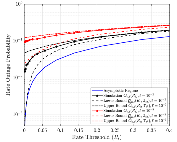
(a) $n=128$

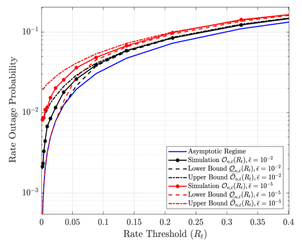
(b) $n=2048$

Figure 1: The rate outage probability versus $(R_{t})$ for $\rho_{o}=-60\ \text{dBm}$, and $\sigma_{w}^{2}=-90\ \text{dBm}$

$$\hat{M}_{b}=\mathbb{E}\left(\mathbb{\hat{P}}_{s}(R_{t},n,\bar{\epsilon})^{b}\right)$$

$$=\int_{0}^{\infty}2\pi\lambda r_{0}\exp\left\{-\pi\lambda r_{0}^{2}-\int_{r_{0}}^{\infty}\frac{2\gamma\left(1+\alpha,\pi\lambda(\rho_{o}w)^{\frac{2}{\eta(1-\alpha)}}\right)}{(\pi\lambda)^{\alpha-1}\rho_{o}^{\frac{-2}{\eta}}\eta w^{1-\frac{2}{\eta}}}\left(1-\left(\frac{p}{1+\frac{\theta)r_{0}^{\eta(1-\alpha)}}{\rho_{o}w}}+(1-p)\right)^{b}\right)e^{\frac{-\theta bN_{0}}{\rho_{o}r_{0}^{-\eta(1-\alpha)}}}dw\right\},$$ (13)

Proposition 2.

The conditional success probability can be lower bounded by

$$\mathbb{\hat{P}}_{s}(R_{t},n,\bar{\epsilon})=\prod_{r_{i}\in\zeta\setminus\{r_{0}\}}\left(\frac{p}{1+\frac{\theta P_{i}r_{i}^{-\eta}}{\rho_{o}r_{0}^{-\eta(1-\alpha)}}}+(1-p)\right)e^{\frac{-\theta N_{0}}{\rho_{o}r_{0}^{-\eta(1-\alpha)}}},$$ (14)

where $\theta=2^{R_{t}+a_{n,\bar{\epsilon}}(\infty)-b_{n}}-1$. Using (14) and the Beta distribution approximation, the meta distribution in (11) can be approximated as

$$\hat{F}_{R_{t}}(p_{th},n,\bar{\epsilon})\approx$$

$$\hskip 14.22636pt1-I_{p_{th}}\left(\frac{\hat{M}_{1}(\hat{M}_{1}-\hat{M}_{2})}{(\hat{M}_{2}-\hat{M}_{1}^{2})},\frac{(1-\hat{M}_{1})(\hat{M}_{1}-\hat{M}_{2})}{(\hat{M}_{2}-\hat{M}_{1}^{2})}\right),$$ (15)

where $I_{z}(x,y)=\frac{1}{\text{B}(x,y)}\int_{0}^{z}t^{x-1}(1-t)^{y-1}dt$ is the regularized incomplete Beta function, and the $\hat{M}_{1}$ and $\hat{M}_{2}$ are the moments of $\mathbb{\hat{P}}_{s}(R_{t},n,\bar{\epsilon})$ provided in (III-B) at the top of next page.

Proof.

Starting from (III-B), we upper bound the $\sqrt{V(\Omega)}$ by $\log_{2}(e)$ which is considered a simple yet convenient bound (it quickly approaches $\log_{2}(e)$ as $\Omega$ increases), leading to $\mathbb{P}_{s}(R_{t},n,\bar{\epsilon})\geq\mathbb{\hat{P}}_{s}(R_{t},n,\bar{\epsilon})$ where

$$\mathbb{\hat{P}}_{s}(R_{t},n,\bar{\epsilon}) =\mathbb{P}^{!}\left(\log_{2}(1+\Omega)-a_{n,\bar{\epsilon}}(\infty)+b_{n}>R_{t}|\zeta\right).$$

Consequently,

$$\mathbb{\hat{P}}_{s}(R_{t},n,\bar{\epsilon})=\mathbb{P}^{!}\left(\Omega>\theta|\zeta\right)$$

$$=\mathbb{E}_{h_{i},x_{i}}\left\{\prod_{r_{i}\in\zeta\setminus\{r_{0}\}}e^{\frac{-\theta x_{i}|h_{i}|^{2}P_{i}r_{i}^{-\eta}}{\rho_{o}r_{0}^{-\eta(1-\alpha)}}}\right\}e^{\frac{-\theta N_{0}}{\rho_{o}r_{0}^{-\eta(1-\alpha)}}},$$

By averaging over the channel gains, we obtain (14). The moments of $\mathbb{\hat{P}}_{s}(R_{t},n,\bar{\epsilon})$ are given in (III-B). Substituting these moments in the Beta distribution (12) yields (2). ∎

IV Numerical Results

We consider a network with intensity $\lambda=2\ \text{BSs}/\text{km}^{2}$, power control parameter $\rho_{o}=\{-60\}\ \text{dBm}$, and path loss exponent $\eta=4$. All the results are validated using Monte Carlo simulations. In the simulation scenario, we set one PPP realization for the BSs in an area of $30\times 30\ \rm{km}^{2}$ area. One UE is placed uniformly within the coverage of each BS.

For the outage probability, we vary the network and the fading realization and calculate the instantaneous SINR $\Omega$ and the instantaneous rate $R_{n,\bar{\epsilon}}(\Omega)$. Then, we compare the instantaneous rate to the rate threshold $R_{t}$ and average to evaluate the outage probability. Further, we numerically optimize the bounds at each $R_{t}$ to optimally choose $\Lambda$ and $\Upsilon$. In Fig. 1, the rate outage probability is plotted versus $R_{t}$ for $n=\{128,2048\}$ and target FER $\bar{\epsilon}\in\{10^{-2},10^{-5}\}$. As shown in the figure, the rate outage upper and lower bounds in (1) and (1) are tight bounds on the performance of the network especially at moderate to high $R_{t}$. It is worth noting that the proposed upper bound provides a guaranteed performance at all values of $R_{t}$ and can be used as an approximation for moderate to high $R_{t}$. While it is evident that a gap exists between the rate outage probabilities in the AR and FBR, quantifying and investigating the behavior of this gap is essential. This gap is due to the term $\sqrt{\frac{V(\Omega}{n}}Q^{-1}(\epsilon)$, which is a function of SINR, which in turn depends on the network scale and density. When the SINR is high/low the $V(\Omega)$ increases/decreases, increasing/decreasing the gap between the FBR and the AR performance. However, the SINR is random and hence the gap needs to be characterized. This gap increases as the target FER $\bar{\epsilon}$ becomes more stringent and the blocklength $n$ becomes shorter, which makes the rate outage probability in the AR for short blocklengths (e.g. $n=128$) misleading, which motivates the analysis in FBR. Moreover, it is noticed that as the blocklength increases the rate outage decreases approaching the performance in the AR.

To investigate the performance of the simplified bound provided in Corollary 1, the simplified upper bound versus $R_{t}$ is plotted in Fig. 2 with the optimized upper bound and the exact performance of the network. The simplified upper bound provides a simple expression that can be easily evaluated but it is not tight for low $R_{t}$. However, for moderate $R_{t}$, it is shown to be tight and can be used as an approximation. The tightness of this bound at moderate to large $R_{t}$ and the existence of a gap between the exact outage probability and the bound is explained next.

In Fig. 1 and 2, it is observed that a gap exists between the optimized bounds and the exact outage probability of the network. This gap increases at low $R_{t}$ and diminishes at moderate to high $R_{t}$. Hence, an analysis is conducted to gain insights into the behavior of this gap and to investigate the significance of the parameters $\Upsilon$ and $\Lambda$, and their impact on the outage probability. We start with the outage definition, where $\mathcal{O}_{n,\bar{\epsilon}}(R_{t})=\mathbb{P}(R_{n,\bar{\epsilon}}(\Omega)<R_{t})=\mathbb{P}(C(\Omega)<R_{t}+a_{n,\bar{\epsilon}}(\Omega)-b_{n})$. The outage probability is calculated by integrating the the pdf of the SINR $\Omega$ such that $C(\Omega)<R_{t}+a_{n,\bar{\epsilon}}(\Omega)-b_{n}$. Hence, we plotted the capacity $C(\Omega)$ and the term $R_{t}+a_{n,\bar{\epsilon}}(\Omega)-b_{n}$ as functions of SINR $\Omega$ in Fig. 3. The term $R_{t}+a_{n,\bar{\epsilon}}(\Omega)-b_{n}$ increases from $R_{t}-b_{n}$ to $R_{t}+a_{n,\bar{\epsilon}}(\infty)-b_{n}$ as SINR increases. To simplify our analysis, we upper bound this function by a step function that changes value from $R_{t}+a_{n,\bar{\epsilon}}(\Upsilon)-b_{n}$ to $R_{t}+a_{n,\bar{\epsilon}}(\infty)-b_{n}$ at $\Upsilon$, which is also plotted in Fig. 3 for optimized values of $\Upsilon$. It is worth noting that the optimal $\Upsilon$ is chosen numerically such that $\bar{\mathcal{O}}_{n,\bar{\epsilon}}(R_{t},\infty)$ is minimized. For small $R_{t}$, we find that the approximating step function overestimates the region at the optimal choice of $\Upsilon$, leading to an integration over undesired region thus increasing the gap between the bound and the actual outage probability. For moderate to large $R_{t}$, the point of intersection of the approximated step function and the capacity approximately matches with the point of intersection of the two exact curves for any choice of $\Upsilon$. Hence, it does not overestimate the integration interval. The significance of $\Upsilon$ is evident at low $R_{t}$. However, its impact is negligible at moderate to high $R_{t}$ which justifies the tightness of the simplified bounds. For the lower bound, the same argument can be made.

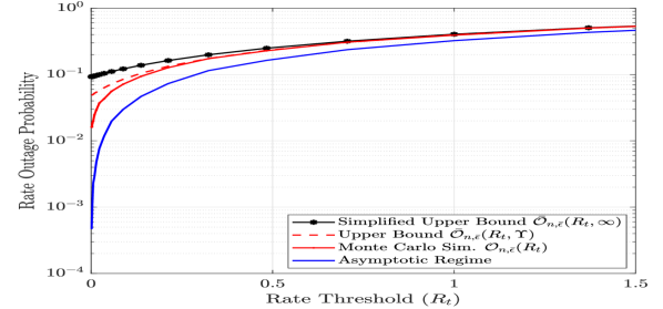
Figure 2: Outage Probability versus $R_{t}$ at $n=128$ and $\epsilon=10^{-2}$

For the meta-distribution of the coding rate simulation, (2) is compared to a simulation with fixed BSs and UEs realizations, and the fading realization changes at each time slot and each user becomes active with probability $\delta$. The SINR is evaluated for the active users and the simulation runs until $20,000$ samples of SINR are collected for each UE, which are used to evaluate per UE coding rate. The meta-distribution of the coding rate is then evaluated across all UEs. In Fig. 4, the coding rate meta distribution is plotted versus $p_{th}$ for rate thresholds $R_{t}\in\{0.5,1.2,1.5\}$ bits/transmission. It is shown that the approximation provided in (2) tightly characterizes the exact coding rate meta distribution for a broad range of $R_{t}$. However, for small $R_{t}$, the approximation provides a lower bound to the coding rate meta-distribution. It is worth noting that, for all $R_{t}$, the approximated meta-distribution provides an achievable performance, meaning it is always guaranteed since it is always below the exact meta distribution. Also, it is shown that the coding rate meta distribution in the AR significantly overestimates the number of users achieving the rate threshold $R_{t}$, by $20\%$ to $40\%$. Hence, our analysis is more precise in estimating the users’ performance.

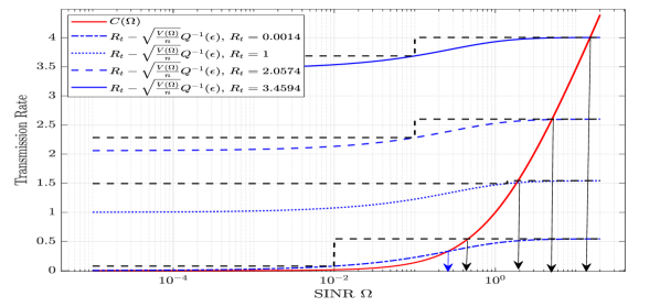
Figure 3: Outage Probability Analysis

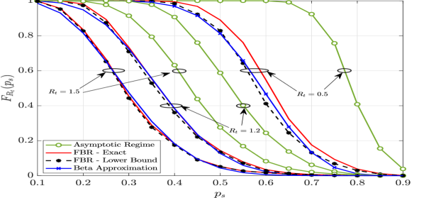
Figure 4: Rate meta distribution versus $p_{th}$ for $n=128$, $\lambda=2\ \text{BS}/\text{Km}^{2}$, $\bar{\epsilon}=10^{-5}$, $\alpha=1$, and $\delta=0.7$

V Conclusion

We studied the performance of large-scale UL networks in the FBR in terms of the rate outage probability and the coding rate meta-distribution where bounds and approximations for both of them are proposed. Numerical results were provided to highlight the tightness of the rate outage probability upper and lower bound. Moreover, we provided a qualitative analysis for the performance of the bounds. Also, the coding rate meta-distribution approximation tightly characterizes the performance in the FBR for a large-scale network. It is also shown that the performance in the AR underestimates the rate outage probability and overestimates the coding rate meta distribution, compared to the realistic performance of the network in the FBR, and the gap is quantified. However, as the blocklength $n$ increases, the performance approaches the performance of the AR. In conclusion, our results can accurately depict the performance of large-scale networks in the FBR.

Appendix A Laplace Transform of the Aggregate Interference Power

By definition, the Laplace transform of $\mathcal{I}$ is given by

$$\mathcal{L}_{\mathcal{I}}(s) =\mathbb{E}\left(\exp\left\{-s\sum_{r_{i}\in\Phi\setminus\{r_{0}\}}x_{i}{P_{i}}|h_{i}|^{2}r_{i}^{-\eta}\right\}\right).$$

The interference coming from the interfering UE point process $\{\Phi\setminus u_{0}\}$ can be approximated with the interference seen from a non-homogeneous PPP $\tilde{\Phi}={\color[rgb]{0,0,0}\{}z_{i}\ ;i\in\mathbb{N}\}$ with intensity function $\lambda_{\text{\tiny{UE}}}(z)=\left(1-e^{-\pi\lambda||z||^{2}}\right)\lambda$, where $z_{i}$ is the vector coordinates of the UEs and $\lambda_{\text{\tiny{UE}}}(z)$ models the intensity of UEs as a function of UE’s location $z$ [5]. To simplify the analysis, we define $w=\frac{||z||^{\eta}}{P}$. Then, for an arbitrary realization, $w_{i}=\frac{||z_{i}||^{\eta}}{P_{i}}$ where $w_{i}\in\tilde{\Phi}_{o}$ and follows a PPP with the following intensity function [5]

$$\lambda(w)=\frac{2(\pi\lambda)^{1-\alpha}\rho_{o}^{\frac{2}{\eta}}}{\eta w^{1-\frac{2}{\eta}}}\gamma\left(1+\alpha,\pi\lambda(\rho_{o}w)^{\frac{2}{\eta(1-\alpha)}}\right),$$ (16)

which is obtained by the Displacement and Mapping Theoreoms for the PPP [10, Theorems 2.33 & 2.34]. Hence, the Laplace transform of interference is given by

$$\mathcal{L}_{\mathcal{I}}(s) =\mathbb{E}\left(\exp\left\{\sum_{w_{i}\in\tilde{\Phi}\setminus\{r_{0}\}}\frac{-sx_{i}|h_{i}|^{2}}{w_{i}}\right\}\right)$$

$$=\exp\left\{-\int_{\frac{r_{0}^{\eta(1-\alpha)}}{\rho_{o}}}^{\infty}\lambda(w)\left(1-\mathbb{E}\left(e^{\frac{-sx|h|^{2}}{w}}\right)\right)dw\right\}$$

$$=\exp\left\{-\int_{\frac{r_{0}^{\eta(1-\alpha)}}{\rho_{o}}}^{\infty}\lambda(w)\left(1-\frac{\delta w}{w+{s}}-(1-\delta)\right)dw\right\}$$

$$=\exp\left\{-\int_{\frac{r_{0}^{\eta(1-\alpha)}}{\rho_{o}}}^{\infty}\lambda(w)\left(\frac{\delta s}{w+{s}}\right)dw\right\}$$ (17)

By substituting (16) in (A), we get (3).

Appendix B Rate Outage Probability Upper Bound

The rate outage probability is given by

$$\mathcal{O}_{n,\bar{\epsilon}}(R_{t}) =\mathbb{P}\left(\log_{2}(1+\Omega)-\frac{\sqrt{V(\Omega)}Q^{-1}(\bar{\epsilon})}{\sqrt{n}}+b_{n}<R_{t}\right)$$

Define $a_{n,\bar{\epsilon}}(x)=\sqrt{\frac{V(x)}{n}}Q^{-1}(\bar{\epsilon})$ Noting that $a_{n,\bar{\epsilon}}(x)$ is an increasing function of $x$, then for any $\Upsilon>0$ we have

$$\mathcal{O}_{n,\bar{\epsilon}}(R_{t}) =\int_{0}^{\Upsilon}\mathbb{P}(\Omega)\mathbb{1}(R_{n,\bar{\epsilon}}(\Omega)<R_{t})d\Omega$$

$$\hskip 45.52458pt+\int_{\Upsilon}^{\infty}\mathbb{P}(\Omega)\mathbb{1}(R_{n,\bar{\epsilon}}(\Omega)<R_{t})d\Omega$$

$$\leq\int_{0}^{\Upsilon}\mathbb{P}(\Omega)\mathbb{1}(\log_{2}(1+\Omega)-a_{n,\bar{\epsilon}}(\Upsilon)+b_{n}<R_{t})d\Omega$$

$$+\int_{\Upsilon}^{\infty}\mathbb{P}(\Omega)\mathbb{1}(\log_{2}(1+\Omega)-a_{n,\bar{\epsilon}}(\infty)+b_{n}<R_{t})d\Omega$$

Hence, the rate outage probability is upper bounded by

$$\bar{\mathcal{O}}_{n,\bar{\epsilon}}(R_{t},\Upsilon) =\int_{0}^{\beta_{1}}\mathbb{P}(\Omega)d\Omega+\int_{\Upsilon}^{\beta_{2}}\mathbb{P}(\Omega)d\Omega$$

$$=\mathbb{F}_{\Omega}(\beta_{1})+\mathbb{F}_{\Omega}(\beta_{2})-{\color[rgb]{0,0,0}\mathbb{F}_{\Omega}(\Upsilon)}$$

for any $\Upsilon>0$, where $\beta_{1}=\min(\Upsilon,2^{R_{t}+a_{n,\bar{\epsilon}}(\Upsilon)-b_{n}}-1)$ and $\beta_{2}=\max(\Upsilon,2^{R_{t}+a_{n,\bar{\epsilon}}(\infty)-b_{n}}-1)$. This concludes the derivation and leads to the result in (1).

Appendix C Rate Outage Probability Lower Bound

The rate outage probability is given by $\mathcal{O}_{n,\bar{\epsilon}}(R_{t})=\mathbb{P}\left(R_{n,\bar{\epsilon}}(\Omega)<R_{t}\right)$. Then, since $a_{n,\bar{\epsilon}}(x)$ is increasing in $x$, for any $\Lambda>0$ we have

$${\mathcal{O}}_{n,\bar{\epsilon}}(R_{t})=\int_{0}^{\Lambda}\mathbb{P}_{\Omega}(\Omega)\mathbb{1}(R_{n,\bar{\epsilon}}(\Omega)<R_{t})d\Omega$$

$$\hskip 85.35826pt+\int_{\Lambda}^{\infty}\mathbb{P}_{\Omega}(\Omega)\mathbb{1}(R_{n,\bar{\epsilon}}(\Omega)<R_{t})d\Omega$$

$$\geq\int_{0}^{\Lambda}\mathbb{P}_{\Omega}(\Omega)\mathbb{1}(\log_{2}(1+\Omega)-a_{n,\bar{\bar{\epsilon}}}(0)+b_{n}<R_{t})d\Omega$$

$$+\int_{\Lambda}^{\infty}\mathbb{P}_{\Omega}(\Omega)\mathbb{1}(\log_{2}(1+\Omega)-a_{n,\bar{\bar{\epsilon}}}(\Lambda)+b_{n}<R_{t})d\Omega.$$

Define $\mu_{1}=\min(\Lambda,2^{R_{t}-b_{n}}-1)$ and $\mu_{2}=\max(\Lambda,2^{R_{t}+a_{n,\bar{\epsilon}}(\Lambda)-b_{n}}-1)$, and since $a_{n,\bar{\bar{\epsilon}}}(0)=0$, the rate outage probability is lower bounded by

$$\underline{\mathcal{O}}_{n,\bar{\epsilon}}(R_{t}) =\int_{0}^{\mu_{1}}\mathbb{P}_{\Omega}(\Omega)d\Omega+\int_{\Lambda}^{\mu_{2}}\mathbb{P}_{\Omega}(\Omega)d\Omega\ \ \$$

$$=\mathbb{F}_{\Omega}(\mu_{1})-\mathbb{F}_{\Omega}(\Lambda)+\mathbb{F}_{\Omega}(\mu_{2}),$$

for any $\Lambda>0$.This concludes the derivation and leads to (1).

References

• [1] Y. Polyanskiy, H. V. Poor, and S. Verdú, “Channel coding rate in the finite blocklength regime,” IEEE Trans. Inf. Theory, vol. 56, no. 5, pp. 2307–2359, 2010.
• [2] W. Yang, G. Durisi, T. Koch, and Y. Polyanskiy, “Block-fading channels at finite blocklength,” in Int. Symp. Wireless Commun. Syst., 2013, pp. 1–4.
• [3] H. ElSawy and E. Hossain, “On stochastic geometry modeling of cellular uplink transmission with truncated channel inversion power control,” IEEE Trans. Wireless Commun., vol. 13, no. 8, pp. 4454–4469, 2014.
• [4] S. Singh, X. Zhang, and J. G. Andrews, “Joint rate and SINR coverage analysis for decoupled uplink-downlink biased cell associations in HetNets,” IEEE Trans. Wireless Commun., vol. 14, no. 10, pp. 5360–5373, 2015.
• [5] H. ElSawy and M.-S. Alouini, “On the meta distribution of coverage probability in uplink cellular networks,” IEEE Commun. Lett., vol. 21, no. 7, pp. 1625–1628, 2017.
• [6] Y. Wang, M. Haenggi, and Z. Tan, “The meta distribution of the SIR for cellular networks with power control,” IEEE Trans. Commun., vol. 66, no. 4, pp. 1745–1757, 2018.
• [7] N. Hesham, A. Chaaban, H. ElSawy, and J. Hossain, “Finite blocklength regime performance of downlink large scale networks,” IEEE Transactions on Wireless Communications, pp. 1–1, 2023.
• [8] Y. Xie, P. Ren, and D. Xu, “On the uplink transmission performance of URLLC with interference channel,” in IEEE Annu. Int. Symp. Personal Indoor Mobile Radio Commun., 2020, pp. 1–6.
• [9] J. G. Andrews, F. Baccelli, and R. K. Ganti, “A tractable approach to coverage and rate in cellular networks,” IEEE Trans. Commun., vol. 59, no. 11, pp. 3122–3134, 2011.
• [10] M. Haenggi, Stochastic Geometry for Wireless Networks.   Cambridge University Press, 2012.