pinned system
Effect of the presence of pinned particles on the structural parameters of a liquid and correlation between structure and dynamics at the local level
Abstract
Pinning particles at the equilibrium configuration of the liquid is expected not to affect the structure and any property that depends on the structure while slowing down the dynamics. This leads to a breakdown of the structure dynamics correlation. Here, we calculate two structural quantities, the pair excess entropy, , and the mean field caging potential, the inverse of which is our structural order parameter (SOP). We show that when the pinned particles are treated the same way as the mobile particles, both and SOP of the mobile particles remain the same as that of the unpinned system, and the structure dynamics correlation decreases with an increase in pinning density, “c”. However, when we treat the pinned particles as a different species, even if we consider that the structure does not change, the expression of and SOP changes. The microscopic expressions show that interaction between a pinned and mobile particle affects and SOP more than the interaction between two mobile particles. We show that a similar effect is also present in the calculation of the excess entropy and the primary reason for the well-known vanishing of the configurational entropy at high temperatures. We further show that contrary to common belief, the pinning process does change the structure. When these two effects are considered, both and SOP decrease with an increase in “c”, and the correlation between the structural parameters and the dynamics continues even for higher values of “c”.
I Introduction
When a glass forming liquid is cooled fast enough, it avoids the crystallization process, and the viscosity/relaxation timescale shows a dramatic increase stillinger ; binder_kob_book . There have been debates about the origin of this increase in viscosity/relaxation time. There are theories suggesting that the slowing down of the dynamics is purely kinetic in nature chandler . However, phenomenological Adam-Gibbs (AG) theory predicts a relation between the relaxation time, , and configurational entropy, , where is a system dependent constant and is the high temperature relaxation time. As predicted by Kauzman many years ago, vanishes at the Kauzmann temperature, , which is a finite temperature below the glass transition temperature Kauzmann . For many systems, the AG relation is found to be valid, and the predicted temperature where the dynamics diverges is found to be the same as adam-gibbs_hold1 ; Adam-Gibbs_hold2 ; Adam-Gibbs_hold3 ; adam-Gibbs_hold4 ; adam-gibbs_hold5 ; adam-gibbs_hold6 ; adam-gibbs_hold7 ; adam-gibbs_hold8 ; adam-gibbs_hold9 . The random first-order transition theory (RFOT), suggests that the slowing down of the dynamics is related to a growing length scale in the system krikpatrick_1989 ; biroli_bouchaud ; wolynes_JCP_2003 which in turn is related to the configurational entropy, of the system thus suggesting a generalized AG relationship cammarota_JCP_2009 ; cavagna_JCP_2012 . However, the ideal glass transition temperature can be obtained only via extrapolating the temperature dependence of to low temperatures.
In order to access the ideal glass transition temperature, , a novel model system was proposed where some fraction of particles in their equilibrium liquid configuration are pinned Biroli_phase_diagram ; walter_original_pinning ; smarajit_chandan_dasgupta_original_pinning ; palak_ujjwal_JCP ; parisi_jamming_pinned_system . It was predicted Biroli_phase_diagram and also shown in numerical simulationswalter_original_pinning ; smarajit_chandan_dasgupta_original_pinning that as the fraction of pinned particles increases, the increases, and eventually, at high enough pinning, the ideal glass transition moves to high enough temperature where the system can be equilibrated. Interestingly, the pinned system can also be experimentally realized by laser pinning some particlespaddy or via soft pinning smarjit_soft_pinnng .
Studies showed that for these pinned systems, although the configurational entropy vanishes at high temperatures, the dynamics continues and there is a breakdown of the AG relationship walter_original_pinning ; reply_by_chandan_dasgupata ; palak_ujjwal_JCP . It was later shown that in the calculation of the vibrational entropy, when anaharmonic contributions are considered, the configurational entropy remains positive walter_anh . However, even with this anharmonic contribution, the AG relationship was shown to break down palak_ujjwal_JCP . It was also shown that the RFOT theory, which leads to a generalized AG relationship, is valid if it is assumed that the configurational entropy of the pinned system is related to the unpinned system by a multiplicative factor where the factor decreases with increasing pinning. smarajit_chandan_dasgupta_original_pinning ; chakrabarty_2016 . All these studies showed that the correlation between dynamics and entropy of the pinned system differs from that of the unpinned systems.
The correlation between local pair excess entropy, which depends on the structure and the local dynamics of the pinned system, was also studied paddy . It was shown that since the pinning process is expected not to affect the structure, the local pair excess entropy remains the same as the unpinned system, whereas the dynamics slows down due to pinning. Thus, there is a decorrelation between pair excess entropy and dynamics even at the microscopic level.
From the above discussion, it appears that both at macroscopic and microscopic levels, the dynamics and the entropy are not correlated. However, at the macroscopic level, pinning decreases the configurational entropy more than slowing down the dynamics walter_original_pinning , whereas, at the microscopic level, the pinning process does not alter the pair excess entropy but slows down the dynamics. Thus, the decorrelation between entropy and dynamics observed at the macroscopic and microscopic levels is just the opposite. Note that for the unpinned system, the macroscopic pair excess entropy, contributes to of the excess entropy Goel_2008 . The configurational entropy has a contribution from three terms: the ideal gas entropy , the excess entropy, and the vibrational entropy, . Since pair excess entropy does not change due to pinning, we can expect the excess entropy, which is usually obtained using thermodynamic integration (TI) method Frankel_n_smith ; ozawa_thesis also not to change. In that case, we may expect that the other terms are responsible for the observed decrease in the configurational entropy of the pinned systems.
In this paper, we first revisit the calculation of the configurational entropy. We show that the decrease in the excess entropy is primarily responsible for the decrease in the configurational entropy. We further show that in the calculation of the excess entropy, the pinned particles should be treated as a different species, and the analytical expression shows that compared to the interaction with another mobile particle, the interaction with a pinned particle contributes twice in decreasing the excess entropy of a mobile particle. We next show that when we use a similar methodology in the calculation of the pair excess entropy, both at macroscopic and microscopic levels, it decreases with pinning. The expression of the pair excess entropy shows that this decrease again comes from the stronger interaction between the pinned and mobile particles.
We then extend the recently developed theoretical formulation, where we describe that each particle in a mean field caging potential for the pinned system. Note that, as shown before, this mean field caging potential is obtained from the structure of the liquid manoj_PRL_2021 ; mohit_PRE ; mohit_wca_lj . We find that even the mean field potential, both at microscopic and macroscopic levels, shows that the pinned particles have a stronger interaction with the mobile particles, thus increasing the depth of the caging potential and confining the mobile particles. We refer to the inverse depth of the caging potential as the structural order parameter(SOP). Interestingly, a similar confinement effect of the pinned particles was observed in the elastically collective nonlinear equation (ECNLE) theory schweizer_phan ; Phan_2022 . In ECNLE theory, the dynamics of the system was obtained using Langevin dynamics on the dynamic free energy surface. The studies showed that with pinning, the depth of the free energy barrier increases, and the particles are more confined. In the ECNLE theory, while treating the system, the Authors considered that the pinned particles do not change the structure, but the pinned particles are considered to be a different species. Thus, it appears that in any formulation to obtain the stronger confinement effect by the pinned particles, the pinned particles should be treated as a different species.
We next show that contrary to the common belief, the pinning process does change the structure, which can be observed only when the partial radial distribution functions are calculated, assuming the pinned particles are a different species. Our study reveals that with an increase in pinning, it is a combined effect of the change in structure and the stronger contribution of pinned particles in decreasing the potential energy of the mobile partciles that reduces both and SOP, the latter effect playing a more dominant role. Finally, we show that the correlation between the local structural parameters ( and SOP) and local dynamics increases when the above mentioned two effects are taken into consideration in the calculation of and SOP.
The rest of the paper is organized as follows: section II contains the simulation details. The analysis at the macroscopic level is presented in section III with excess entropy, , in section III.1, pair excess entropy, , in section III.2, the depth of local caging potential, , in section III.3 and the numerical results in section III.4. The analysis at the microscopic level is presented in section IV with microscopic in section IV.1, microscopic in section IV.2 and numerical results in section IV.3. In section V, we analyze the structure dynamics correlation at the microscopic level. The paper ends with a brief conclusion in section VI. This paper contains six Appendix sections at the end.
II Simulation Details
In this study, we work with the well-known Kob-Andersenkob-andersen 80:20 binary Lenard-Jones mixture. The shifted and truncated Lennard-Jones interaction potential in the KA model is given by,
| (1) |
where and . Where and = 1.0, = 1.5, = 0.5, = 1.0, = 0.80, = 0.88. Length, energy, and time scales are measured in units of , and , respectively. We use three-dimensional, Lammps-based molecular dynamics simulationlammps . The Nosé-Hoover thermostat is used to simulate NVT molecular dynamics in a cubic box with N = 4000, = 1.2, integration time step = 0.005. The system is equilibrated for a period longer than 100 , where is the system’s relaxation time.
The following pinning procedure is applied to create the pinned system. The pinned particles are chosen randomly from an equilibrium configuration of the KA system at the target temperaturewalter_berthier_pin_2013 ; smarajit_chandan_dasgupta_original_pinning . In this process, we make sure that the ratio of mobile A and mobile B particles in the pin sub-population is the same as the regular KA system (80:20). Note that we ensure that two pin particles are not close to each other. The simulations are performed assuming that there is no interaction between two pinned particles (). After pinning, we perform NVT molecular dynamics simulation with an integration time step = 0.005. We equilibrate the system for . For this work, we generate three different pinning concentrations “c”, i.e., 0.05, 0.10, and 0.15.
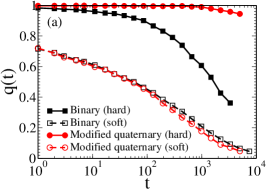
In this work, to characterize the dynamics, we consider the self part of the overlap function, q(t), defined as;
| (2) |
where function when and otherwise. The overlap parameter cutoff (a) = 0.3 is taken such that particle positions separated due to small amplitude vibrational motion are treated as the sameoverlap_shiladitya . We calculate the relaxation time by examining the time where the overlap function decays to 1/e = 0.367.
III Entropy and mean field caging potential at macroscopic level
III.1 Macroscopic excess entropy
The excess entropy of a system is the loss of entropy due to the interaction between particles. The excess entropy of pinned systems has been calculated before, and it was also shown that compared to the unpinned system, the configurational entropy of the system disappears at a higher temperature walter_original_pinning ; palak_ujjwal_JCP . As discussed in the Introduction, this disappearance of the configurational entropy at a temperature where the dynamics continues has been a topic of intense research walter_original_pinning ; smarajit_chandan_dasgupta_original_pinning ; reply_by_chandan_dasgupata ; reply_by_kob ; palak_ujjwal_JCP . The configurational entropy, is obtained from the ideal gas entropy, , excess entropy, and the vibrational entropy, of the system. All these three terms change due to pinning. Here, we first revisit the configurational entropy calculation and find out which terms are primarily responsible for the vanishing of the configurational entropy of the pinned system at a higher temperaturewalter_original_pinning ; Biroli_phase_diagram . As shown in Appendix II we find that as we increase the pinning concentration, the per particle ideal gas entropy increases. However, the per particle excess entropy and per particle vibrational entropy decrease. The decrease in the excess entropy appears to be stronger than the vibrational entropy. We make a comparative analysis of the excess entropy of the pinned and the unpinned systems to understand what leads to this substantial decrease in the excess entropy.
The excess entropy per particle level is expressed asFrankel_n_smith ; ozawa_thesis ;
| (3) |
where is per partial potential energy.
In the case of a regular binary system, the per particle potential energy in terms of the radial distribution function, g(r), can be expressed asHansen_and_McDonald :
| (4) | ||||
where, is the fraction of particles in type . N is the total number of particles in the system.
Note that when we pin particles in a binary system, we actually create a quaternary system of two types of mobile particles and two types of pinned particles. We refer to the first type of mobile particles as species 1, the second type of mobile particles as species 2, the first type of pinned particles as species 3, and the second type of pinned particles as species 4. The potential energy per particle for a regular quaternary system can be expressed as follows:
| (5) | ||||
Now if we assume that a fraction, of particles are pinned then . The number of mobile particles can be written as . In our model system, the pinned particles do not interact with each otherwalter_original_pinning ; thus, . We also know that the interaction between pinned and mobile particles is symmetric, for example, . These conditions modify the quaternary expression and reduce the first summation in Eq. 5 only over types 1 and 2. Moreover, for a system with pinned particles, the excess entropy, , is calculated only for the mobile particles, and the total potential energy is divided only between the mobile particles. This further modifies the quaternary expression (Eq. 5), and the potential energy at per mobile particle level for the pinned system, which we now also refer to as the modified quaternary system, can be written as;
| (6) | ||||
The above expression of the potential energy, when replaced in Eq. 3, provides us with the excess entropy of the mobile particles in the pinned system, . The first and second terms in Eq. 6 describe the potential energy of a mobile particle due to the interaction with other mobile particles and pinned particles, respectively. The expression of the first and second term are identical except for the fact that the 2nd term has a factor of 2. This implies that compared to a mobile particle, a pinned particle has a stronger effect in decreasing the potential energy of a mobile particle. In Appendix II, we show that if we neglect this stronger effect of the pinned particles on the mobile particle i.e. remove the factor 2 in the second term of (Eq. 6) then the excess entropy shows a marginal change and the per particle configurational entropy increases with an increase in pinning density. This is because, with the increase in pinning density, the increase in the ideal gas entropy is more than the decrease in the vibrational entropy. This result is not physical, but it clearly shows that the vanishing of the configurational entropy at higher temperatures is due to the stronger effect of the pinned particles in confining the mobile particles and thus decreasing the excess entropy. We will show in section III.2 and III.3 that this effect of the pinned particles plays an important role in the two body excess entropy and the mean field caging potential.
III.2 Macroscopic pair excess entropy
The excess entropy, can be written in terms of an infinite series via the Kirkwood factorization methodKirkwood ; Green_N_body_correlation_1958 ,
| (7) |
While represents the loss of entropy due to total interaction, the pair excess entropy, describes the loss of entropy due to interaction described by the two-body correlation. is the loss of entropy due to many body correlations (beyond pair correlation). The per particle pair excess entropy, which contributes to 80% of the total excess entropyGoel_2008 can be written asGreen_N_body_correlation_1958 ;
| (8) |
Pair excess entropy per particle level for the quaternary system is expressed as;
| (9) |
To obtain the pair excess entropy of the pinned system, , we make similar modifications to the pure quaternary system as is done for the calculation of the excess entropy given in the previous system. First, we assume that there is no structure between the pinned particles, i.e. . This assumption is justified as , and we can also neglect any higher order correlation between the pinned particles, thus assuming that the potential of mean force between the pinned particles also vanishes. We also assume that the partial rdf between mobile and pinned particles is symmetric. Thus, the first summation in Eq. 9 is only over the mobile particles, types 1 and 2. Next, in the modified system, we calculate the entropy of only the mobile particles. The total pair excess entropy, is divided only amongst the mobile particles, and the per particle pair excess entropy of the mobile particles, . Thus, in the first summation is replaced by like in Eq. 6. The pair excess entropy per particle level of the mobile particles in the pinned system, can be written as,
| (10) |
From Eq. 10, we find that similar to that discussed for excess entropy, when we treat the pinned system as this modified quaternary system, the effect of the pinned particles in determining the entropy of the mobile particles is stronger (factor of 2) compared to other mobile particles.
When we pin the particles at their equilibrium position, the structure/rdf of the system is not expected to change. Thus, pinning is believed to keep the equilibrium of the system the samePaddy_article ; paddy ; walter_wall_pinning_paper . If the structure/rdf remains the same, then treating the system as quaternary or binary in the calculation of the two body excess entropy gives us identical results, (see Appendix III). However, note that for the pinned system, the pair excess entropy is not given by (Eq. 9) but by (Eq. 10). In the expression of , even if we assume there is no change in structure due to pinning, the pair excess entropy of the system, is different from that of a binary system and can be written as,
| (11) |
Note that in writing the last equality, we have applied the relation, and . Thus, it shows that even if the pinning process does not change the structure, the pair excess entropy for mobile particles in the pinned system is lower than that in the unpinned system. This implies that the pinned particles have a stronger confinement effect on the mobile particle. In the next section, we will show that this stronger confining effect of the pinned particles is present not only in entropy but also in other quantities.
III.3 Macroscopic mean field caging potential
The time evolution of the density, under mean-field approximation, can be written in terms of a Smoluchowski equation in an effective mean field caging potential, which is obtained from the Ramakrishnan-Yussouff free energy functionalManoj_prl_2017 ; manoj_PRL_2021 ; mohit_PRE . Following our earlier studies, the caging potential is calculated by assuming that the cage is static when the particle moves by a distance manoj_PRL_2021 . The mean field caging potential is expressed in terms of the static structure factor/radial distribution function of the liquid mohit_PRE . In this section, we obtain a pinned system’s mean field caging potential. Previous work by some of us showed that the depth of caging potential is coupled to the dynamicsmanoj_PRL_2021 ; mohit_PRE . Thus, in this study, instead of dealing with the whole potential, we deal with the absolute magnitude of the depth of the caging potential as we view the depth of the caging potential as an energy barrier. We first start with the binary system, where the average depth of mean field caging potential can be expressed asmohit_PRE ;
| (12) |
Here is the separation between the tagged particle and its neighbors and , , is the density. is the tagged particle’s distance from its equilibrium position. According to Hypernetted chain approximation, the direct correlation function, , can be represented as;
| (13) |
For a regular quaternary system, the caging potential can be expressed as;
| (14) |
Next, for the calculation of the mean field caging potential for the pinned system, we apply similar conditions as discussed before for the calculation of the excess and pair excess entropies. Under these conditions the average depth of mean field caging potential of the mobile particles in the pinned system, can be written as;
| (15) |
Note that similar to excess and pair excess entropy, the depth of the mean field caging potential of mobile particles in this modified quaternary system is affected more by the pinned particles (factor of 2) than by other mobile particles. Also, if the structure does not change due to pinning, the expression of the caging potential for a quaternary and binary system is identical, but that is not the case for the modified quaternary system. The expression for the depth of the mean field caging potential under the assumption that the structure does not change due to pinning can be written as,
| (16) |
In the last equality we have applied the relation that and . The above expression suggests that even when we assume that the structure does not change due to pinning, the depth of the caging potential for the pinned system is deeper compared to the unpinned system. This higher confinement effect comes due to the stronger interaction with the pinned particles. Interestingly, a similar effect of the pinned particles has been discussed while studying the nonlinear Langevin equation on a dynamic free energy surface schweizer_phan ; Phan_2022 . Note that our mean field caging potential is obtained from the functional derivative of the static version of this dynamic free energy schweizer_2005 ; Manoj_prl_2017 . Similar to the methodology used here, their study, schweizer_phan ; Phan_2022 on a monoatomic liquid treats the pinned system as a binary system, thus considering the pinned particle as a different species. They also consider the dynamic free energy of only the mobile particles. Under these conditions, they show that the free energy barrier and confinement of the mobile particles increase with pinning density.
III.4 Numerical results for the macroscopic pair excess entropy and mean field caging potential
Note that the two body excess entropy and the mean field caging potential are both functions of the radial distribution function (rdf) given by,
| (17) |
where V is the system’s volume, , are the number of particles of the and types, respectively. , are the and particle’s position in the system respectively.
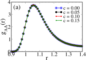
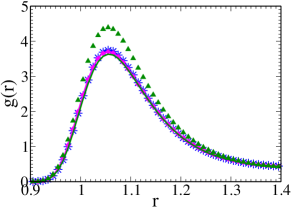
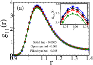
In Fig. 1, we plot the partial rdfs of the system where we do not differentiate between the pinned and unpinned particles and we find that, as expected, the rdf remains the same as the unpinned regular KA model (c=0).

In the rest of the article when we refer to the unpinned binary KA system, following the usual norm, we refer to the particles as A and B types. However, as discussed in the previous sections, when we pin particles in a binary system, we actually create a quaternary system. We refer to the mobile A type of particles as 1, mobile B type of particles as 2, pinned A type of particles as 3, and pinned B type of particles as 4.
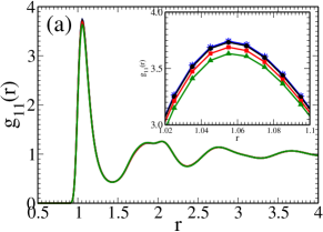
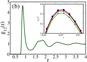
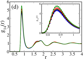
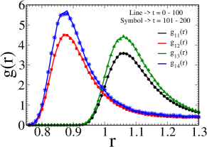
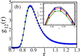
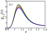
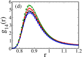
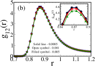
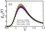
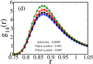
We next plot some representative partial rdfs assuming the system to be quaternary at different pinning concentrations (Fig. 2). We find that with increased pinning density, the partial rdfs start deviating from the c=0 system. With an increase in “c”, there is a drop in the peak value of the rdfs between two mobile particles (, ). On the other hand, the first peak height of the partial rdfs between mobile and pinned particles (, ) grows with “c”. To ensure that this is not an art effect of choosing the pinned particles as a different species, in the c=0 system, we randomly choose 15% of the particles and treat them as a different species. In Fig. 3, we show that in that case, . A similar result is also observed for other partial rdfs (not shown here). This clearly shows that when we pin a certain fraction of particles, contrary to the common belief, there is a structural change.
We observe that this structural change happens quickly, immediately after the pinning process. We calculate , averaged from and , where the pinning is performed at t=0. We find that both rdfs overlap (Appendix IV, Fig. 13). In Appendix IV, Fig. 14, we also show that is the same as and is the same as . This is precisely why we do not see a change in structure when the pinned particles are not treated as a different species (Fig. 1). Note that this change in the partial rdfs is independent of the integration timestep and system size (Fig. 16).

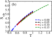
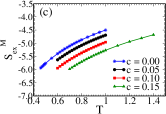
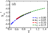
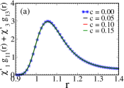
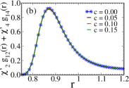
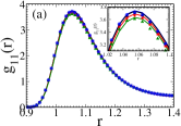
Thus, from this analysis, it is clear that the structure of the system does change when particles are pinned. However, this change is significant at higher pinning densities only when we treat the pinned particles as a different species. In Fig. 4, we plot the pair excess entropy, (Eq. 11) and the caging potential, (Eq. 16) of the pinned systems where we assume that the structure does not change due to pinning. We also plot (Fig. 4 (a)) and (Fig. 4 (b)), where we consider that the structure changes due to pinning. We find that, even when we consider that the structure does not change, the pair excess entropy of the pinned system differs from that of the binary system and decreases with increasing pinning density. This decrease in entropy is due to the stronger effect of the pinned particles in confining the mobile particles. When we consider that the structure changes due to pinning, as shown in Fig. 2, then the entropy further decreases, and like the structure, this decrease is significant at higher pinning densities. The plot of the mean field caging potential shows a similar effect. The caging potential depth increases with pinning, even if the change in the structure due to pinning is ignored. There is a further increase in the depth when the change in the structure is taken into account.
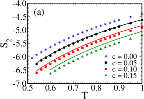
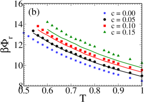
Thus, we find that both the pair excess entropy and the mean field caging potential for the pinned system differ from that of the unpinned system, and this difference comes due to two factors. Firstly, compared to the interaction between two mobile particles, the interaction between a mobile and a pinned particle is stronger, leading to a decrease in entropy and an increase in the caging potential. Secondly, due to pinning, the structure of the liquid changes, and this further decreases the entropy and increases the mean field caging potential. As seen from Fig. 4, the first effect is stronger and plays a dominant role.
In Appendix III, we show that the well-known crossoverAtreyee_2017 between the excess entropy and the pair excess entropy takes place at a physically meaningful temperature only when we take into consideration these two effects in the calculation of the entropy.
IV Pair excess entropy and mean field caging potential at the microscopic level
In the previous section, we developed the protocol for calculating the caging potential and pair excess entropy at the macroscopic level for the pinned system. However, our primary goal is to understand how these two order parameters can describe the dynamics at the local level. We clearly demonstrate that the pinned system should be treated as a modified quaternary system. In this section, we make a comparative analysis of these two structural quantities, when the pinned system is treated as a binary system and a modified quaternary system. First, we start with the microscopic expressions, which are obtained from the macroscopic expressions. The bigger “A” particles, which are larger in number, are the ones for which all microscopic calculations are performed. This is done to make sure that there is no size inhomogeneity, which we know also affects the dynamicspalak_polydisperse_softness .
IV.1 Microscopic pair excess entropy
Calculation of the pair excess entropy at the macroscopic level () is given in section III.
In the binary system, the pair excess entropy of each mobile “A” particle, which is type “1” in our notation, can be expressed by removing the first summation in Eq. 8;
| (18) |
Similarly, in the modified quaternary system, the pair excess entropy of each mobile “A” particle (type 1) can be expressed by removing the first summation in Eq. 10;
| (19) |
Note that the differences between the binary and modified quaternary are the following. In the binary expression, when treating the neighbors, we do not differentiate between the mobile and pinned particles; however, in the quaternary expression, we do. Thus, in the binary expression, the effect of the mobile neighbors on the tagged particle is the same as that of the pinned neighbors. However, in the quaternary expression, the effect of the pinned neighbors on the tagged particle is twice that of the mobile neighbors. As shown in the macroscopic calculation (Fig. 4), it is this second effect that plays a dominant role in differentiating between the binary and the modified quaternary values of the entropy.
IV.2 Microscopic mean field caging potential
The macroscopic calculation of the depth of the caging potential (), the inverse of which we refer to as the structural order parameter (SOP), is given in section III.3. At the microscopic level for a binary system, the caging potential of a mobile “A” type of particle can be written by removing the first summation in Eq. 12;
| (20) |
The mean field caging potential for a mobile “A” type of particle in a modified quaternary system can be written by removing the first summation in Eq. 15,
| (21) |
Thus, note that similar to that discussed for the pair excess entropy, in the modified quaternary expression, compared to the mobile neighbors, the pinned neighbors have a stronger effect in confining the tagged particle.
IV.3 Numerical results for the microscopic pair excess entropy and mean field caging potential
To perform the microscopic investigation, we determine and for every snapshot at the single particle level that requires the partial rdfs to be calculated at a single particle level. In this calculation, the sum of Gaussian can be used to express the single particle partial rdf in a single frame, and it is calculated as followspiggi_PRL ;
| (22) |
where “” is the particle index, is the density. The Gaussian distribution’s variance () is employed to transform the discontinuous function into a continuous form. We use for this work. Single particle rdf is used to derive the direct correlation function at the single particle level from Eq. 13.
We can determine caging potential (Eq. 12, 14, 15) by combining the direct correlation function (Eq. 13) and particle level rdf (Eq. 22). This leads to a term that is a product of the interaction potential and the rdf. As shown in an earlier workmohit_PRE , at distances shorter than the average rdf, the particle level rdf generated by the Gaussian approximation has finite values. At small “r” due to this finite value of the rdf, its product with the interaction potential, which diverges at small “r”, leads to a large unphysical contribution from this range. To get around this problem, we use an approximate expression of the direct correlation function, where we assume that the interaction potential is equal to the potential of mean force . It has also been shown earlier that using marginally improves the theoretical prediction of structure-dynamics correlationpalak_polydisperse_softness ; mohit_wca_lj . In the rest of the microscopic calculation, we will use in place of .
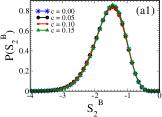
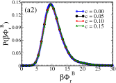
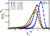
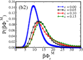
In Fig. 5, we plot the distribution of pair excess entropy and local caging potential by describing the pinned system as binary. Note that for all the cases, the quantities are calculated only for the mobile “A” particles. We find that the distribution remains similar to the unpinned system (KA model at c=0). This is because the expressions are identical for pinned and unpinned systems, and even for c=0.15, there are enough mobile “A” particles to give the correct statistics. However, when we calculate the quantities assuming the pinned system as a modified quaternary system (Eq. 15 and 10), we observe that as “c” increases, the depth of the caging potential increases and the pair excess entropy decreases. Distribution of , and are shown in Fig. 5. This analysis clearly shows that the entropy and the SOP (inverse depth of the caging potential) are higher when the system is treated as binary compared to when it is treated as a modified quaternary. In the next section, we will show that the correlation between the dynamics and structural quantities differs when we treat the pinned system as binary or modified quarternary.
V Correlation between structure and dynamics at microscopic level
In the following section, we study the correlation between two structural order parameters, namely the and SOP, with the dynamics using different techniques. To make a comparative analysis, while calculating the structural quantities, we treat the pinned system both as binary and modified quaternary systems.
V.1 Correlation between structure and dynamics using isoconfiguration runs
In this section, we study the correlation between structure and dynamics using isoconfiguration runs (IC). IC is a powerful technique developed by Harrowell et al.Cooper_IC_2004 ; Cooper_IC_2006 ; Harowell ; Bertheir_IC to examine the role the structure plays in the dynamics (details are given in Appendix V).
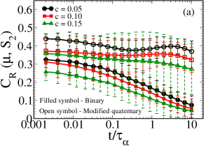
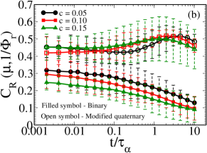
We calculate the Spearman rank correlation, (where = - is the difference between the ranks, and of the raw data and respectively, and m denotes the number of data), between the mobility, and the pair excess entropy ()), and between the mobility, and the SOP . In Figs. 6(a) and 6(b), we plot and respectively, for the pinned systems as a function of scaled time. We observe that when considering the system as a binary system, the correlations, and ) decrease as the pinning concentration increases (Fig. 6). This observation is concurrent with the findings of Williams et al.paddy . However, when the system is treated as a modified quaternary system, we observe an increase in and compared to when the system is treated as binary. This suggests that treating the system as binary does not capture the full complexity of the structure-dynamics relationship. In the modified quaternary treatment of the system, the pinning decreases the pair excess entropy and the SOP, which is commensurate with the slowing down of the dynamics.
Between the SOP and the pair excess entropy, we find that the SOP can predict the dynamics better and . This is similar to that observed in an earlier study where, for attractive systems compared to entropy, the SOP is a better predictor of the dynamics mohit_wca_lj . Also note that for all values of “c”, the peak height of the almost remains constant, whereas the peak height of drops with an increase in “c”. Thus the difference between and increases with “c”. This drop in the value of with an increase in “c” may be connected to the breakdown of the AG relationship at the macroscopic level. However, we cannot calculate the configurational entropy at the microscopic level, but we do find from Fig. 5 that the shift in the distribution of the pair excess entropy with pinning density is stronger than the shift in the distribution of SOP.
We also find that with increasing pinning concentration, the peak height of ) moves to smaller values of . A similar observation was made while comparing the more fragile Lennard-Jones (LJ) and the less fragile Weeks-Chandler-Anderson (WCA) modelsmohit_wca_lj . Note that in the case of pinned systems, the fragility decreases with increasing “c”smarajit_chandan_dasgupta_original_pinning . Thus, it appears that for more fragile systems, the correlation between structure and dynamics continues for longer times. However, at this point, this is only a conjecture, and to make more concrete statements, further investigations are needed, which is beyond the scope of the present study.
V.2 Analysis of dynamics of particles belonging to the softest and hardest regions
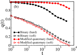
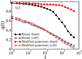
Since we show that the inverse of the mean field caging potential, SOP, is a better predictor of the dynamics, in the next two subsections, we will present the study of the structure-dynamics correlation using only the SOP. At short timescales, we expect to observe a significant difference in the dynamics of the hardest (in a deep cage) and softest (in a shallow cage) particles. The hardest particles, less likely to escape their local cages, will exhibit slower dynamics. On the other hand, the softest particles, with a higher probability of moving, will display faster dynamics. However, over a longer time, as the cage evolves, the separation in dynamics between the hardest and softest particles diminishesmohit_PRE ; manoj_PRL_2021 ; palak_polydisperse_softness . We average over a few (approximately 2-3) hardest and softest particles and compare their dynamics via the overlap function (Eq. 2). Note that the identity of the soft and hard particles depends on how the SOP is calculated, i.e. assuming the system to be binary or modified quaternary.
The dynamics of the hardest and softest particle for different concentrations of the pinning is shown in Fig. 7. When we calculate the SOP treating the system as a modified quaternary system, the difference in dynamics between the hard and the soft particles is wider compared to the case where the system is treated as binary (Fig. 7). Note that the difference is greater for the hard particles. This is because our analysis reveals that the identity of the softest particles does not change when we treat the system as binary or modified quaternary. However, the identity of the hardest particles completely changes because, in the binary treatment, we neglect the stronger interaction between the pinned and the mobile particles, which is present in the modified quaternary treatment. Due to this effect in the modified quaternary treatment, the hardest particles are the ones that have pinned particles as their neighbors. As shown in Fig. 7, the hardest particles, as identified by the modified quaternary treatment, are slower than those identified by the binary treatment. This is precisely the reason why the modified quaternary treatment of the system shows higher value of compared to the binary treatment of the system.
V.3 Correlation between structure and dynamics and prediction of onset temperature
In this section, we use the structure dynamics correlation to identify the onset temperature of the glassy dynamics, a methodology used in earlier studiesAndrea_liu_nature ; mohit_PRE .
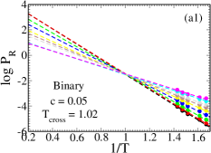
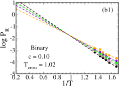
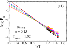
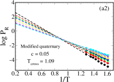
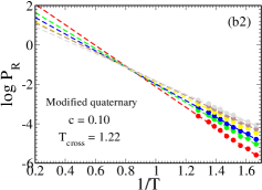
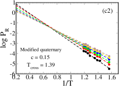
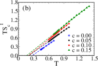
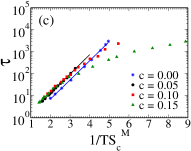
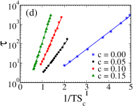
We identify fast particles using a well-documented methodCandelier_PRL ; smessaert_PRE ; mohit_PRE (details are given in Appendix VI). In Fig. 8 we plot as a function of temperature for different values and find that it can be expressed in an Arrhenius form, , where activation energy, is a function of and is higher for smaller values. The plots cross at a certain temperature, which describes the limiting temperature where the theory is validmohit_PRE and has been identified earlier as the onset temperature of the supercooled liquidAndrea_liu_nature ; mohit_PRE ; palak_polydisperse_softness .
In this analysis, we find that when we treat the system as binary, the onset temperature remains similar for all pinning concentrations. However, when we treat the system as a modified quaternary system, the onset temperature increases with increasing pinning concentrationBiroli_phase_diagram . As we show in Appendix I, this predicted onset temperature is similar to the onset temperature predicted from the well known inherent structure energy method (Fig. 9 and Table 1)sastry_inherent_1998 .
VI Conclusion
As discussed in the Introduction, earlier studies on the pinned system have shown that both at macroscopic and microscopic levels, the correlation between the dynamics and entropy breaks down. However, the nature of the breakdown at the microscopic and macroscopic levels is not similar but just the opposite. At the macroscopic level, with pinning, the configurational entropy disappears, whereas the dynamics continues walter_original_pinning ; palak_ujjwal_JCP ; reply_by_chandan_dasgupata . At the microscopic level, the pair excess entropy remains high and the same as the unpinned system, whereas the dynamics slows down with an increase in pinning density paddy . This is possible only when the macroscopic configurational entropy and the microscopic pair excess entropy are uncorrelated. However, it is well known that for the unpinned systems, the pair excess entropy contributes to about of the excess entropy, which in turn contributes to the configurational entropy Goel_2008 . Thus, to understand the different results at the macroscopic and microscopic levels, we revisit the excess entropy calculation of the pinned system.
We show that when we pin particles in a binary system, we should treat this pinned system as a quaternary system under the assumption that there is no interaction between pinned particles (an assumption we use while simulating the system) and the potential energy is only distributed amongst the mobile particles. The excess entropy of this modified quaternary system predicts that the effect of a pinned particle in stabilizing a mobile particle by decreasing the potential energy is a factor of two more than the effect of another mobile particle. We show that this effect leads to the well documented vanishing of configurational entropy at higher temperaturesBiroli_phase_diagram and the breakdown of the Adam-Gibbs relationship in a pinned systemwalter_original_pinning ; palak_ujjwal_JCP .
We follow the same methodology to calculate the pair excess entropy and the mean field caging potential at macroscopic and microscopic levels. We first show that the expression of and SOP (inverse depth of the mean field caging potential) differ when the system is treated as binary and modified quaternary. In the binary treatment, the effect of a pinned particle on the mobile particle is identical to that of another mobile particle. However, in modified quaternary treatment, similar to that observed in the calculation of the excess entropy, the pinned particles have a stronger effect on the mobile particles than other mobile particles. We next show that contrary to the common belief that if pinned at the equilibrium position, the properties of the system do not change, pinning changes the structure of the liquid, which can be observed only when we treat the pinned particles as a different species. We then show that when we treat the system as a modified quaternary system, the entropy and the SOP are much lower than that obtained by treating the system as a binary system. The analysis reveals that more than the change in structure, the stronger effect of the pinned particles on the mobile particles plays a dominant role in confining the mobile particles by decreasing the entropy and the SOP. Interestingly, a similar confinement effect of the pinned particles was discussed in an earlier study of a monotonic system, where it was shown that the free energy barrier of the mobile particles increases with pinning densityschweizer_phan ; Phan_2022 . Note that similar to the the present study in these earlier studiesschweizer_phan ; Phan_2022 , the pinned particles were treated as a different species.
We further study the correlation between structure and dynamics using different techniques. In all cases, we show that compared to the case where the pinned system is treated as a binary system, there is an increased correlation between structural order parameters and the dynamics when the pinned system is treated as a modified quaternary system. This is because, unlike in the binary case, in the modified quaternary case, the pinned particles affect not only the dynamics but also the structural properties. We also show that compared to the entropy, the SOP can predict the dynamics better. The correlation between fast particles and the SOP can only predict the correct onset temperature when the SOP is calculated, assuming the pinned system is a modified quaternary system.
In Summary, our study reveals two important points. The pinning affects not only the bulk macroscopic quantities but also the microscopic quantities. The effect of the pinned particles can be expressed by treating the pinned particles as a different species, which then shows that a pinned particle confines the mobile particle more than another mobile particle which then alters the microscopic expression of the quantities that depend on the structure. Thus, pinning not only slows down the dynamics of the mobile particle but also changes the structural parameters.
Along with this, the pinning process also affects the structure of the liquid. In future studies, these two effects should be considered when calculating different properties of the pinned system. Also, note that, like local pair excess entropy, the local mean field caging potential depends on the local structure. This allows us to apply it to experimental colloidal systems where, both for quiescent and sheared systems, we find a good structure dynamics correlation rati . Thus, the mean field caging potential can be applied to study the structure-dynamics correlation even in experimental pinned systems paddy ; smarjit_soft_pinnng .
Appendix I: Onset temperatures of the pinned systems from inherent structure energy
To estimate the temperature range of the system, we first obtain the onset temperature of the supercooled. In Fig. 9, we plot the inherent structure energy, as a function of T to calculate the onset temperature () from the inherent structure (IS)sastry_inherent_1998 . at different pinning concentrations is given in Table 1. The IS is obtained using the FIRE algorithmFIRE_method_for_inherent_str . From this analysis, we observe that the onset temperature increases with increasing pinning concentration, “c”Biroli_phase_diagram (see Table 1).
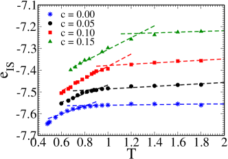
| c | |
|---|---|
| 0.00 | 0.80 |
| 0.05 | 0.89 |
| 0.10 | 1.01 |
| 0.15 | 1.27 |
Appendix II: Various forms of entropy in pinned systems
The various forms of entropy in pinned systems are discussed here.
-
•
Ideal gas entropy: The ideal gas entropy in pinned systems only comes from the moving particle. The pinned system’s ideal gas entropy is calculated aswalter_original_pinning ;
(23) where is the total number of particles that are moving and is the de Broglie thermal wavelength and h is the Planck constant. We plot the per particle ideal gas entropy of pinned systems at various pinning concentrations in Fig. 10. As the pinning increases, we see an increase in ideal gas entropy. The decrease in the density (as ) and the increase in the mixing entropy contribute to the increase in the per particle ideal gas entropy.
-
•
Vibrational entropy: We consider a weakly vibrating system around an inherent structure (IS). If we indicate by the displacement of the particle from its point in the IS, then the potential energy can be approximated well by the following formulawalter_original_pinning ,
(24) It is important to realize that only the derivative of the potential energy with respect to the coordinates of unpinned particles should be taken into account, not including the ones of pinned particles. (However, of course U will depend on the positions of the pinned and unpinned particles). Thus, the size of the Hessian matrix is . Introducing the eigenvalues of the Hessian, the harmonic vibrational entropy of the given inherent structure with a given pinned particle configuration can be written aswalter_original_pinning ;
(25) We plot the vibrational entropy of pinned systems at various pinning concentrations in Fig. 10. As the pinning increases, we see a drop in vibrational entropy.
-
•
Excess entropy: We employ the thermodynamic integration approach to determine entropy from simulations. At the target temperature , the entropy of the system with the pinned particles can be written aswalter_original_pinning ; ozawa_thesis ; palak_ujjwal_JCP ;
(26) where is a thermal average of the potential energy. Details of excess entropy calculation are discussed in section III.1. We plot the excess entropy of pinned systems at various pinning concentrations in Fig. 10. As the pinning increases, we see a drop in excess entropy. We also plot the excess entropy for the pinned system where we ignore the stronger effect of the pinned particles on the mobile particles by removing the prefactor 2 in the second term of (Eq. 6), which we now denote as and express as;
(27) In this case, the excess entropy can be written as;
(28) We find that the excess entropy, , does not decrease with pinning. Rather, it shows a marginal increase. This analysis clearly shows that the decrease in the excess entropy with pinning is due to the higher potential energy contribution of the pinned particles, which leads to a stronger confinement of the mobile particles.
In Fig. 11 we plot the configurational entropy, and at different pinning concentrations. We observe that the Kauzmann temperature, , where the extrapolated entropy vanishes, increases when excess entropy is calculated using the modified quaternary expression of the potential energy, and the Adam-Gibbs relation between the dynamics and entropy is not valid. However, when we ignore the stronger effect of the pinned particles on the mobile particle, i.e. use in the calculation of the excess entropy, then decreases with increasing pinning and the Adam-Gibbs relation between the dynamics and entropy is valid. This, as discussed in the main paper, is not a physically correct picture, but this analysis clearly shows that in the pinned system, the vanishing of the entropy at higher temperatures is due to the stronger confinement effect of the pinned particles on the mobile particles.
Appendix III: Pair excess entropy
In section III.2, we show that the pair excess entropy can have different expressions when the system is treated as binary, quaternary, and modified quaternary. We also show that the rdf is different when the system is treated as binary and quaternary (section III.4).
If the structure (rdf) does not change, then treating the system as quaternary or binary in the calculation of the gives us identical results. This can be easily seen when comparing Eq. 8 and Eq. 10. If we assume that in the rdfs we can replace 3 by 1 and 4 by 2 then Eq. 9 can be rewritten as,
| (29) |
The last equality can be written because and .
In Fig. 12 we plot where the change in structure due to the pinned particles is considered. We find that at high temperatures is larger than , and at low temperatures, the scenario is reversed.
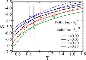
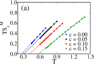
The temperature where these two entropies cross each other is the (Eq. 7) point. For the KA model (c=0) and other systems, it was earlier shown that the temperature where these two entropies cross is similar to the onset temperature of glassy dynamicsAtreyee_2017 ; palak_polydisperse . However, it has also been found that in systems with mean field like characteristics, the temperature where is lower than the onset temperaturemanoj_GCM ; Ujjwal_thesis . The latter scenario is similar to what we find for pinned systems. We find that with the increase in pinning, the difference between the onset temperature and the temperature where the two entropies cross increases. Interestingly, a similar difference between the freezing point and was observed for higher dimensional systemstruskett_delta_s_sign and Gaussian core model (GCM)coslovich_GCM . Note that if the pair excess entropy is calculated assuming the pinned system to be a binary system, then the cross over between the pair excess entropy and the total entropy will take place at unphysically low temperatures.
Appendix IV: Radial distribution function
In Fig. 2 (assuming the pinned particles are of a different species) we find that with increased pinning density, the partial rdfs start deviating from the c=0 system. With an increase in “c”, there is a drop in the peak value of the rdfs between two mobile particles (, ). On the other hand, the height of the first peak of the partial rdfs between mobile and pinned particles (, ) grows with “c”.
We observe that this structural change happens quickly, immediately after the pinning process. In Fig. 13, we plot , averaged from and , where the pinning is done at t=0. We find that both rdfs overlap. This is shown for the c=0.15 system where the difference is maximum.
We also show that is the same as and is the same as (Fig. 14). This is precisely why we do not see a change in structure when the pinned particles are not treated as a different species (Fig. 1).
To check the system size dependence, in Fig. 15, we plot the rdfs for a 4000 particle and 1000 particle system. We find that change in the rdf with pinning is almost independent of the system size, with the difference between the rdfs of the unpinned and pinned systems increasing marginally for larger system sizes.
We also check the dependence of the rdf on the integration time (Fig. 16). From this plot, we observe that rdf is independent of the integration time step.
Appendix V: Isoconfiguration run (IC)
To quantify the dependence of the dynamics on the structure and particle size, we perform isoconfigurational runs (IC). IC is a powerful technique introduced by Harrowell and co-workers to investigate the role of structure in the dynamical heterogeneity of the particlesCooper_IC_2004 ; Cooper_IC_2006 ; Harowell ; Bertheir_IC . Among other factors, a particle’s displacement can depend on its structure and also its initial momenta. This technique was proposed to remove the uninteresting variation in the particle displacements arising from the choice of initial momenta and extract the role of the initial configuration on the dynamics and its heterogeneity. For each system, five different isoconfigurational runs are carried out for 4000 particles. To ensure that all configurations are different, the configurations are chosen such that the two sets are greater than 100 apart. All these five IC has different structure as well as contain different pin particle position. Note that since we have shown in section III.4 that after pinning, the structure changes; thus after we pin the equilibrium position of the mobile particles, we run the system for t=100 timestep and then consider that as our initial configuration. We run 100 trajectories for each configuration with different starting velocities randomly assigned from the Maxwell-Boltzmann distribution for the corresponding temperatures.
Mobility, is the average displacement of each particle over these 100 runs and is calculated asHarowell ,
| (30) |
where particle’s mobility at time is represented by the term . The position of the particle in the trajectory at time is denoted by the term , and its initial position is denoted by the term . The sum of the values is calculated over each of the trajectories that were carried out during the isoconfiguration runs. We determine the average displacement or mobility for the particle at time by averaging these displacements over all trajectories.
Appendix VI: Identification of fast particles
There are various methods available for identifying fast particles in the literaturewalter_PRL_1997 ; walter_JCP_2002 ; Widmer-Cooper_2005 ; Candelier_PRL ; smessaert_PRE . In our study, we employ the approach proposed by Candelier et al.Candelier_PRL ; smessaert_PRE . This method involves the calculation of a quantity called for each particle within a specified time window .
The quantity captures the rate of change in the average position of a particle, indicating the occurrence of a cage jump. The expression for is given as followsAndrea_liu_nature :
| (31) |
here, represents the position of particle , and denote the averages over the time. The time window is divided into two intervals, U = [t - , t] and V = [t, t + ]. By calculating for each particle, we can determine whether a particle experiences a significant change in its average position, indicating its involvement in cage jumps and enhanced dynamics. In our analysis, we compare the calculated values to a threshold value , which is determined as the mean square displacement, at a specific time where the non-Gaussian parameter, is maximized. If exceeds , we identify the particle as a fast particlemohit_PRE ; Andrea_liu_PRE ; palak_polydisperse .
It is important to note that in our study, we specifically analyze the structure and dynamics of the mobile A particles. Therefore, we calculate the Mean Square Displacement (MSD) and the non-Gaussian parameter specifically for the mobile A particles. For a more comprehensive understanding of the method and its application in our study, we refer readers to Referencemohit_PRE ; palak_polydisperse ; Andrea_liu_PRE ; Andrea_liu_nature .
ACKNOWLEDGMENT
P. P. Thanks, CSIR, for the research fellowships. S. M. B. thanks, SERB, for the funding. The authors would like to thank Chandan Dasgupta, Smarajit Karmakar, and Mohit Sharma for the discussions.
AVAILABILITY OF DATA
The data that supports the findings of this study is available from the corresponding author upon reasonable request.
VII Reference
References
- (1) P. G. Debenedetti and F. H. Stillinger, Nature 410, 259 (2001).
- (2) K. Binder and W. Kob, Glassy Materials and Disordered Solids, Revised ed. (WORLD SCIENTIFIC, 2011).
- (3) D. Chandler, D. Wu, and P. Chandler, Introduction to Modern Statistical Mechanics (Oxford University Press, 1987).
- (4) W. Kauzmann, Chemical Reviews 43, 219 (1948).
- (5) C. A. Angell, J Res Natl Inst Stand Technol. 102, 171 (1997).
- (6) R. Richert and C. A. Angell, The Journal of Chemical Physics 108, 9016 (1998).
- (7) J. H. Magill, The Journal of Chemical Physics 47, 2802 (1967).
- (8) T. M. Shuichi Takahara, Osamu Yamamuro, The Journal of Physical Chemistry 99, 9589 (1995).
- (9) K. L. Ngai, The Journal of Physical Chemistry B 103, 5895 (1999).
- (10) C. Alba-Simionesco, Comptes Rendus de l’Académie des Sciences - Series IV - Physics-Astrophysics 2, 203 (2001).
- (11) C. M. Roland, S. Capaccioli, M. Lucchesi, and R. Casalini, The Journal of Chemical Physics 120, 10640 (2004).
- (12) D. Cangialosi, A. Alegría, and J. Colmenero, Europhysics Letters 70, 614 (2005).
- (13) E. Masiewicz et al., Scientific Reports 5, 2045 (2015).
- (14) T. R. Kirkpatrick, D. Thirumalai, and P. G. Wolynes, Physical Review A 40, 1045 (1989).
- (15) G. Biroli and J.-P. Bouchaud, The Random First-Order Transition Theory of Glasses: A Critical Assessment (John Wiley and Sons, Ltd, 2012), chap. 2, pp. 31–113.
- (16) V. Lubchenko and P. G. Wolynes, The Journal of Chemical Physics 119, 9088 (2003).
- (17) C. Cammarota, A. Cavagna, G. Gradenigo, T. S. Grigera, and P. Verrocchio, The Journal of Chemical Physics 131, 194901 (2009).
- (18) A. Cavagna, T. S. Grigera, and P. Verrocchio, The Journal of Chemical Physics 136, 204502 (2012).
- (19) C. Cammarota and G. Biroli, Proceedings of the National Academy of Sciences 109, 8850 (2012).
- (20) M. Ozawa, W. Kob, A. Ikeda, and K. Miyazaki, Proceedings of the National Academy of Sciences 112, 6914 (2015).
- (21) S. Chakrabarty, S. Karmakar, and C. Dasgupta, Scientific Reports 5, 12577 (2015).
- (22) U. K. Nandi et al., The Journal of Chemical Physics 156, 014503 (2022).
- (23) C. Brito, G. Parisi, and F. Zamponi, Soft Matter 9, 8540 (2013).
- (24) I. Williams et al., Journal of Physics: Condensed Matter 30, 094003 (2018).
- (25) R. Das, B. P. Bhowmik, A. B. Puthirath, T. N. Narayanan, and S. Karmakar, PNAS Nexus 2, pgad277 (2023).
- (26) S. Chakrabarty, S. Karmakar, and C. Dasgupta, Proceedings of the National Academy of Sciences 112, E4819 (2015).
- (27) M. Ozawa, A. Ikeda, K. Miyazaki, and W. Kob, Physical Review Letter 121, 205501 (2018).
- (28) S. Chakrabarty, R. Das, S. Karmakar, and C. Dasgupta, The Journal of Chemical Physics 145, 034507 (2016).
- (29) T. Goel, C. N. Patra, T. Mukherjee, and C. Chakravarty, The Journal of Chemical Physics 129, 164904 (2008).
- (30) D. Frenkel and B. Smit, Appendix k - small research projects, in Understanding Molecular Simulation (Second Edition), pp. 581–585, Academic Press, San Diego, , second edition ed., 2002.
- (31) M. Ozawa, Numerical Study of Glassy Systems: Fragility of Supercooled Liquids, Ideal Glass Transition of Randomly Pinned Fluids, and Jamming Transition of Hard Spheres, Thesis (2015).
- (32) M. K. Nandi and S. M. Bhattacharyya, Physical Review Letter 126, 208001 (2021).
- (33) M. Sharma, M. K. Nandi, and S. M. Bhattacharyya, Physical Review E 105, 044604 (2022).
- (34) M. Sharma, M. K. Nandi, and S. Maitra Bhattacharyya, The Journal of Chemical Physics 159, 104502 (2023).
- (35) A. D. Phan and K. S. Schweizer, The Journal of Chemical Physics 148, 054502 (2018).
- (36) A. D. Phan, Journal of Physics: Condensed Matter 34, 435101 (2022).
- (37) W. Kob and H. C. Andersen, Physical Review E 51, 4626 (1995).
- (38) D. Majure et al., Large-Scale Atomic/Molecular Massively Parallel Simulator (LAMMPS) Simulations of the Effects of Chirality and Diameter on the Pullout Force in a Carbon Nanotube Bundle, IEEE , 201 (2008).
- (39) W. Kob and L. Berthier, Physical Review Letter 110, 245702 (2013).
- (40) S. Sengupta, F. Vasconcelos, F. Affouard, and S. Sastry, The Journal of Chemical Physics 135, 194503 (2011).
- (41) M. Ozawa, W. Kob, A. Ikeda, and K. Miyazaki, Proceedings of the National Academy of Sciences 112, E4821 (2015).
- (42) J. P. Hansen and I. R. McDonald, The Theory of Simple Liquids, 2nd ed. ,Academic, London (1986).
- (43) J. G. Kirkwood and E. M. Boggs, The Journal of Chemical Physics 10, 394 (1942).
- (44) R. E. Nettleton and M. S. Green, The Journal of Chemical Physics 29, 1365 (1958).
- (45) C. P. Royall, F. Turci, S. Tatsumi, J. Russo, and J. Robinson, Journal of Physics: Condensed Matter 30, 363001 (2018).
- (46) P. Scheidler, W. Kob, and K. Binder, Journal of Physical Chemistry B 108, 6673 (2004).
- (47) M. K. Nandi, A. Banerjee, C. Dasgupta, and S. M. Bhattacharyya, Physical Review Letter 119, 265502 (2017).
- (48) K. S. Schweizer, The Journal of Chemical Physics 123, 244501 (2005).
- (49) A. Banerjee, M. K. Nandi, S. Sastry, and S. Maitra Bhattacharyya, The Journal of Chemical Physics 147, 024504 (2017).
- (50) P. Patel, M. Sharma, and S. Maitra Bhattacharyya, The Journal of Chemical Physics 159, 044501 (2023).
- (51) P. M. Piaggi, O. Valsson, and M. Parrinello, Physical Review Letter 119, 015701 (2017).
- (52) A. Widmer-Cooper, P. Harrowell, and H. Fynewever, Physical Review Letter 93, 135701 (2004).
- (53) A. Widmer-Cooper and P. Harrowell, Physical Review Letter 96, 185701 (2006).
- (54) A. W. Cooper, H. Perry, P. Harrowell, and D. R. Reichman, Nature Physics 4, 711 (2008).
- (55) L. Berthier and R. L. Jack, Physical Review E 76, 041509 (2007).
- (56) S. S. Schoenholz, E. D. Cubuk, D. M. Sussman, E. Kaxiras, and A. J. Liu, Nature Physics 12 (2016).
- (57) R. Candelier et al., Physical Review Letter 105, 135702 (2010).
- (58) A. Smessaert and J. Rottler, Physical Review E 88, 022314 (2013).
- (59) S. Sastry, P. G. Debenedetti, and F. H. Stillinger, Nature 393, 554 (1998).
- (60) R. Sahu, M. Sharma, P. Schall, S. M. Bhattacharyya, and V. Chikkadi, Under preparation .
- (61) J. Guénolé et al., Computational Materials Science 175, 109584 (2020).
- (62) P. Patel, M. K. Nandi, U. K. Nandi, and S. M. Bhattacharyya, The Journal of Chemical Physics 154, 034503 (2021).
- (63) M. K. Nandi and S. Maitra Bhattacharyya, The Journal of Chemical Physics 148, 034504 (2018).
- (64) U. kumar Nandi, Connecting real glasses to mean-field models: A study of structure, dynamics and thermodynamics, Thesis (2021).
- (65) W. P. Krekelberg, V. K. Shen, J. R. Errington, and T. M. Truskett, The Journal of Chemical Physics 128, 161101 (2008).
- (66) D. Coslovich, A. Ikeda, and K. Miyazaki, Physical Review E 93, 042602 (2016).
- (67) W. Kob, C. Donati, S. J. Plimpton, P. H. Poole, and S. C. Glotzer, Physical Review Letter 79, 2827 (1997).
- (68) K. Vollmayr-Lee, W. Kob, K. Binder, and A. Zippelius, The Journal of Chemical Physics 116, 5158 (2002).
- (69) A. Widmer-Cooper and P. Harrowell, Journal of Physics: Condensed Matter 17, S4025 (2005).
- (70) F. P. Landes, G. Biroli, O. Dauchot, A. J. Liu, and D. R. Reichman, Physical Review E 101, 010602 (2020).