Non-Hermitian Entropy Dynamics in Anyonic Parity-Time Symmetric Systems

Abstract

Parity-Time (PT) symmetry and its spontaneous breaking attracts growing interesting both in theory and experiments. Here we develop a new approach using the generalized non-Hermitian entropy to investigate the information dynamics of PT, anti-PT, and anyonic-PT symmetric systems. Our results reveal three distinguished patterns of information dynamics in different parameter spaces of anti-PT and anyonic-PT symmetric Hamiltonians, respectively, which are three-fold degenerate and distorted if we use the conventional entropy or trace distance adopted in previous works. The fundamental reason for the degeneracy and distortion is found. Our work provides a phenomenological justification for non-Hermitian entropy being negative. We then explore the mathematical reason and physical meaning of the negative entropy in open quantum systems, revealing a strong connection between negative non-Hermitian entropy and negative quantum conditional entropy. Therefore, our work opens up the new journey of rigorously investigating physical interpretations of negative entropy in open quantum systems.

I Introduction

In recent decades, parity-time symmetry and its spontaneous breaking attracts growing interesting both in theory and experiments. On one hand, non-Hermitian (NH) physics with parity-time symmetry can be seen as a complex extension of the conventional quantum mechanics, having novel properties. On the other hand, it closely related to open and dissipative systems of realistic physics [1, 2, 3, 4]. Typical Hon-Hermitian systems include different symmetries, such as the parity-time-reversal (PT) symmetry [5, 6, 7], anti-PT (APT) symmetry [8, 9, 10, 11, 12, 13, 14, 15], pseudo-Hermiticity [16, 17], anyonic-PT symmetry [18, 19, 20]. In the quantum regime, various aspects of PT symmetric systems have been studied, such as entanglement [21, 22, 23], critical phenomena [24], and etc. For a PT symmetric system, the Hamiltonian $H_{{\rm PT}}$ satisfies $[{\rm PT},H_{{\rm PT}}]=0$. It is in PT-unbroken phase if each eigenstate of Hamiltonian is simultaneously the eigenstate of the PT operator, in which case the entire spectrum is real. Otherwise, it is in PT symmetry broken phase, and some pairs of eigenvalues become complex conjugate to each other. Between the two phases lies exceptional points (EPs) where an unconventional phase transition occurs [5, 25, 26], and this is related to many intriguing phenomena [27, 28, 29, 30, 6]. APT symmetry can be seen as the imaginary counterpart of PT symmetry with APT symmetric Hamiltonians $H_{{\rm APT}}$ satisfying $\{{\rm PT},H_{{\rm APT}}\}=0$. A wide array of physical systems have been tailored to exhibit APT symmetry including, but not limited to, diffusive systems [9], dissipatively coupled optical systems [8], flying atoms [10], revealing exotic physical phenomena. Anyonic-PT symmetry can be seen as the complex generalization of PT symmetry and the relationships between PT, APT, and anyonic-PT symmetry can be an analogy to relationships between boson, fermion, and anyon [19, 18, 20]. In this spirit, it was named anyonic-PT symmetry.

While Hermiticity ensures the conservation of probability in an isolated quantum system and guarantees the real spectrum of eigenvalue of energy, it is ubiquitous in nature that the probability in an open quantum system effectively becomes non-conserved due to the flows of energy, particles, and information between the system and the external environment [25]. For a NH open quantum system with density matrix $\Omega(t)$, it is an intrinsic feature of the system that the trace of the density matrix ${\rm Tr}\,\Omega(t)$ varies with time, which origins from the non-unitary time evolution governed by the NH Hamiltonian. In quantum information, the trace of density matrix appears in various formulae describing different properties of a focused system, such as von Neumann entropy [32], Rényi entropy [33, 34] and trace distance measuring the distinguishability of two quantum states [35, 6, 36, 15]. Here comes the question that should we use the normalized or non-normalized density matrix for non-Hermitian system.

In this work, we develop a new approach based on non-normalized density matrix $\Omega(t)$ to investigate the entropy dynamics of typical NH quantum systems. Our results reveal many new information dynamics patterns in different parameter space of APT or anyonic-PT symmetric systems, which properly characterize the dynamical properties of the systems. The new patterns will not be revealed by the approaches of conventional entropy or trace distance dealing only with normalized density matrices, which are adopted in previous works [6, 36, 37, 15]. In details, for PT symmetric systems, our approach not only predicts and finds all the characteristic phenomena in [6], but also characterizes the non-Markovian and Markovian processes more properly than [6]. For APT symmetric systems in PT-broken phase, our results show three information-dynamics patterns: the periodic oscillations with an overall decrease, stable and increase. We find the three patterns will degenerate to the stable one using conventional entropy or trace distance. For APT symmetric systems in PT-unbroken phase, a three-fold degeneracy happens too if we use conventional entropy or trace distance, while three non-degenerate patterns (decreasing, constant and increasing) can be obtained by our approach. For general anyonic-PT symmetric systems, in PT-unbroken or PT-broken phase, our results show that the intertwining of the PT and APT symmetric systems leads to new patterns of information dynamics: the damped oscillations with an overall decrease, stable and increase. The approaches of conventional entropy or trace distance not only degenerate the three distinguished patterns to the same one, but also obviously distort it. We demonstrate that the degeneracy is caused by the normalization of the NH-evolved density matrix. It is the normalization that leads to the loss of information about the total probability flow between the open system and the environment, while our approach based on the non-normalized density matrix reserves all the information related to the NH time-evolution. Apart from the three-fold degeneracy, our results show that the lower bounds of both conventional entropy and trace distance being zero is related to their distortion of the information dynamics of the NH systems, and thus our work can provide a phenomenological justification for the necessity of negative NH entropy. We go one step further and give a phenomenological description of the process that entropy of NH system goes to negative values. Furthermore, we find there is a strong and comprehensible correspondence in the definition of NH entropy and quantum conditional entropy, and both quantities can be negative for similar mathematical reasons. Since the physical interpretation and the following applications of negative quantum conditional entropy are successful and promising [38, 39, 40], we remark that our work opens up the new journey to rigorously investigate the physical interpretations and the application prospects of negative entropy in NH system.

This paper is structured as follows. In section II, for generic PT symmetric systems in finite dimensions with non-degenerate eigenvalues, we discuss the quantum recurrence in PT-unbroken open quantum systems and why the recurrence fails at PT-broken open quantum systems. In section III, we establish the information-theoretic characterization of the PT, APT and anyonic-PT symmetric systems with non-Hermitian entropy $S_{{\rm NH}}$ and find that $-\ln{\rm Tr}\,\Omega(t)$ (negative of the logarithm of ${\rm Tr}\,\Omega(t)$) and $S_{{\rm NH}}$ are highly correlated. In section IV, we compare our approach with the approaches of conventional entropy and trace distance adopted in previous works investigating non-Hermitian systems. We obtain similar results for PT symmetric systems, while new patterns of the entropy dynamics associated with the APT or anyonic-PT symmetric Hamiltonians are revealed by our approach.

II quantum recurrence in PT-unbroken open quantum systems

We work with generic NH Hamiltonians in finite dimensions and assume the eigenvalues are not degenerate. We shall begin with a comment on the proof of quantum recurrence in PT-unbroken open quantum systems and why the recurrence fails at PT-broken open quantum systems. [6] embeds a PT-symmetric system of interest into a larger Hermitian system. Time-independent $H_{{\rm PT}}$ is extended to a Hermitian Time-independent Hamiltonian $H$ by adding a two-level ancilla. [6] proofs that the PT-symmetric system returns to the initial state by applying quantum recurrence theorem [41] to $H$ and quantum measurement acting on the ancilla. The proof begins with the Hermitian invertible operator ${\eta}$ that characterizes the pseudo-Hermiticity of $H_{{\rm PT}}$, satisfying ${\eta}{H}_{\rm PT}={H}_{\rm PT}^{{\dagger}}{\eta}$ [42].

However, [6] didn’t explain why the recurrence fails at PT-broken open quantum systems and made some wrong statements: it is a priori not obvious whether such an extension with a finite-level ancilla is possible, and this underlying finite dimensionality is a nontrivial universal feature of the PT- unbroken open quantum systems. When PT symmetry is broken, in contrast, $\eta$ is no longer Hermitian and the above extension breaks down [6]. Firstly, for a generic non-Hermitian, arbitrary dimensional and time-dependent (or time-independent) Hamiltonian, you can extend the it into a Hermitian Hamiltonian by introducing an ancilla qubit [43]. The problem is not with that the extension with a finite-level ancilla is impossible. When the PT symmetry is broken, we can extend the PT symmetric system to a Hermitian one by introducing an ancilla qubit but the extended Hermitian Hamiltonian will be time-dependent and thus the quantum recurrence theorem fails. Secondly, $\eta$ is always Hermitian with PT symmetry being unbroken or broken. A longer technical account (Zhihang Liu and Chao Zheng, manuscript in preparation), with rigorous proofs will appear in another paper.

Anyonic-PT symmetric Hamiltonians $H_{\varphi}$ satisfy $({\rm PT})H_{\varphi}({\rm PT})^{-1}=e^{\text{i}\varphi}H_{\varphi}$, and thus

$$H_{\varphi}=e^{-\text{i}\frac{\varphi}{2}}H_{{\rm PT}}=\cos\frac{\varphi}{2}H_{{\rm PT}}-\sin\frac{\varphi}{2}(\text{i}H_{{\rm PT}}),$$ (1)

with corresponding $H_{{\rm APT}}=\text{i}H_{{\rm PT}}$. $H_{\varphi}$ allows us to take a unified treatment to $H_{{\rm PT}}$ (when $\varphi=0$) and $H_{{\rm APT}}$ (when $\varphi=-\pi$). For the general case ($H_{\varphi}\neq H_{{\rm PT}}\;{\rm or}\;H_{{\rm APT}}$), new novel phenomena and application prospects emerge. Here we employ the usual Hilbert-Schmidt inner product when we investigate the effective non-unitary dynamics of an open quantum system described by anyonic-PT symmetric non-Hermitian Hamiltonians [6, 44, 45]. The dynamics governed by $H_{\varphi}$ ($H_{{\rm PT}}$, $H_{{\rm APT}}$) is described by

$$U_{\varphi}=e^{-\text{i}H_{\varphi}t/\hbar}$$ (2)

$$\Omega(t)=U_{\varphi}\Omega(0)U_{\varphi}^{\dagger}$$ (3)

$$\rho(t)=\Omega(t)/{\rm Tr}(\Omega(t)),$$ (4)

with $\varphi=0$ for $H_{{\rm PT}}$ and $\varphi=-\pi$ for $H_{{\rm APT}}$. About normalization, in standard quantum mechanics, with initial wave function normalized, the Schrödinger equation automatically preserves the normalization of the wave function. However, in [6, 44, 45], for open quantum systems, with initial condition ${\rm Tr}\,\Omega(0)=1$, the normalization procedure Eq.(4) is artificial rather then intrinsic to the Schrödinger equation. So, in this paper, instead of $\rho(t)$, we focus on $\Omega(t)$.

Setting eigenstate of ${H}_{\rm PT}$ with an eigenenergy $E_{n}+\text{i}\Gamma_{n}$ as $\ket{\varphi_{n}}$,

$${H}_{\rm PT}\ket{\varphi_{n}}=\left(E_{n}+\text{i}\Gamma_{n}\right)\ket{\varphi_{n}}.$$ (5)

The spectral decomposition of the PT dynamics is

$${\Omega}\left(t\right)={\sum_{mn}\Omega_{mn}e^{-\text{i}\omega_{mn}t}\ket{\varphi_{m}}\bra{\varphi_{n}}},$$ (6)

where $\omega_{mn}:=E_{m}-E_{n}+\text{i}(\Gamma_{m}-\Gamma_{n})$. And

$${\rm Tr}\,\Omega(t)={\rm Re}({\sum_{mn}\Omega_{mn}e^{-\text{i}\omega_{mn}t}\braket{\varphi_{n}}{\varphi_{m}}})$$ (7)

with Re meaning the real part of a complex number. With unitary dynamics, eigenstates are orthogonal and ${\rm Tr}\,\Omega(t)$ is unit. In the NH dynamics, when all $\omega_{mn}$ is real (which is the main feature of PT symmetry unbroken), ${\rm Tr}\,\Omega(t)$ oscillates with a certain period due to the non-orthogonality of eigenstates, indicating the total probability flowing between the system and environment. We demonstrate later that the total probability flowing can be used to describe the continuous information exchange between the system and the environment. With $\omega_{mn}$ being real, the period is evaluated as the least common multiple of $2\pi/\omega_{mn}$ ($m,\,n=1,\,2,\,\cdots,\,N$). In contrast, for PT-broken open quantum systems, $\text{i}(\Gamma_{m}-\Gamma_{n})$ is not zero and thus ${\rm Tr}\,\Omega(t)$ no longer oscillates.

III non-Hermitian entropy

In units Boltzmann constant $k_{B}=1$, non-Hermitian entropy [47] is defined as:

$$S_{{\rm NH}}(\Omega)=-{\rm Tr}(\rho\ln\Omega)$$ (8)

Considering a non-Hermitian Hamiltonian $H=H_{0}-i\Gamma$, where both $H_{0}$ and $\Gamma$ are Hermitian, under gauge transformation $\Gamma=\Gamma^{\prime}+\frac{1}{2}\hbar\alpha I$ (it is evident that the difference of eigenenergies is invariant under the gauge transformation), von Neumann entropy $S_{{\rm vN}}(\rho)=-{\rm Tr}(\rho\ln\rho)$ stays the same, i.e., information regarding the shifting $\frac{1}{2}\alpha I$ is lost, while non-Hermitian entropy $S_{{\rm NH}}$ can reflect the transformation [47].

$$S_{{\rm NH}}=S_{{\rm NH}}^{\prime}+\alpha t$$ (9)

To get the analytical expression of $S_{{\rm NH}}$, since we already have the expression of $-\ln{\rm Tr}(\Omega)$, the formula [47] $S_{{\rm NH}}=-\ln{\rm Tr}(\Omega)+S_{{\rm vN}}$ transforms the problem into calculating of $S_{{\rm vN}}$. Intuition inspires us to investigate the relationship between $S_{{\rm NH}}(\Omega)$ and $-\ln{{\rm Tr}(\Omega)}$ and we show below that the two quantities are highly correlated.

We consider generic two-level systems to demonstrate our analysis and results. For all figures in this paper (in units $\hbar=1$), the red line represents the non-Hermitian entropy $S_{{\rm NH}}\,\Omega(t)$ (the left vertical axis) , the dashed blue line represents the $-\ln{{\rm Tr}(\Omega(t))}$ (the right vertical axis), and the scales of left and right vertical axes are set to be same.

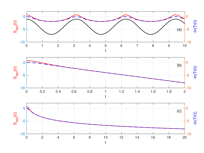
Figure 1: parameter setting: $r_{1}=2$, $\theta_{1}=\pi/6$. (a) $r=2\sqrt{3}$, $\delta=1$, $\Delta_{{\rm PT}}=2\sqrt{\delta}=2$, PT symmetry unbroken. The black line represents $-{\rm Tr}(\Omega(t))$, which shows why we adopt $-\ln{{\rm Tr}(\Omega(t))}$. (b) $r=4\sqrt{2}$, $\delta=-4$, $\Delta_{{\rm PT}}=2\sqrt{\delta}=4\text{i}$, PT symmetry broken. (c) $r=4$, $\delta=0$, $\Delta_{{\rm PT}}=2\sqrt{\delta}=0$, system at exceptional point. The three dynamical patterns of $S_{{\rm NH}}$ are well predicted by the expressions of trace.

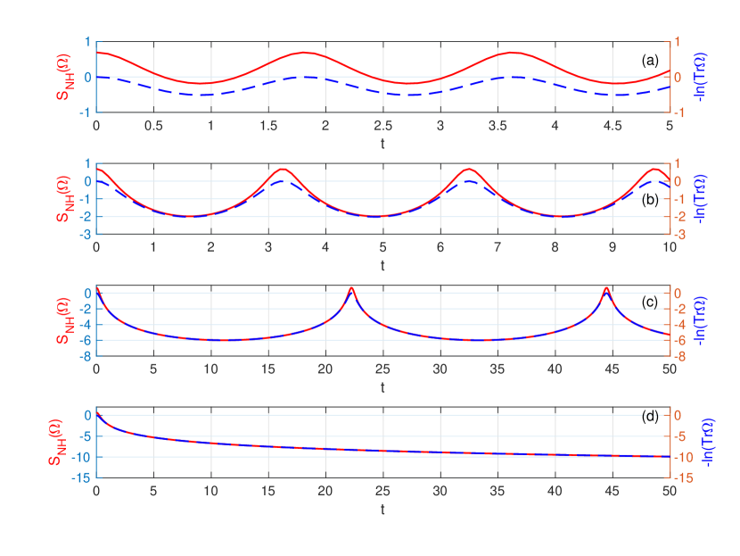
Figure 2: parameter setting: $r_{1}=2$, $\theta_{1}=\pi/6$. (a) $r=2$, $\delta=3$, $\Delta_{{\rm PT}}=2\sqrt{\delta}=2\sqrt{3}$, (b) $r=3.5$, $\delta=\frac{15}{16}$, $\Delta_{{\rm PT}}=2\sqrt{\delta}=\frac{\sqrt{15}}{2}$, (c) $r=3.99$, $\delta=0.02$, $\Delta_{{\rm PT}}=2\sqrt{\delta}=0.04$, system in the vicinity of exceptional point. (d) $r=4$, $\delta=0$, $\Delta_{{\rm PT}}=2\sqrt{\delta}=0$, system at exceptional point.

For a PT symmetric system, fig.(1) shows that complete information retrieval from the environment can be achieved in the PT-unbroken phase, whereas no information can be retrieved in the PT-broken phase. The exceptional point thus marks the reversible-irreversible criticality of information flow. When PT symmetry is unbroken, several phenomena showed in fig.(2) deserve attention. Firstly, the correlation between $S_{{\rm NH}}\,\Omega(t)$ and $-\ln{{\rm Tr}\,\Omega(t)}$ becomes stronger as the system getting closer to exceptional point. Secondly, the monotonic decrease in the non-Hermitian entropy ($\frac{\partial}{\partial t}S_{{\rm NH}}<0$) represents unidirectional information flow from the system to the environment and thus the dynamics is considered to be Markovian. In contrast, an increase in the non-Hermitian entropy ($\frac{\partial}{\partial t}S_{{\rm NH}}>0$) represents information backflow from the environment to the system, implying the presence of memory effects in the open quantum dynamics and that complete information retrieval from the environment can be achieved in the PT-unbroken phase. In other words, the dynamics involving a time interval with $\frac{\partial}{\partial t}S_{{\rm NH}}>0$ is considered to be non-Markovian [48, 49, 50, 51, 52, 53, 54, 55, 56]. Thirdly, unconventional criticality of information flow emerges in the vicinity of exceptional point. Here we give a reason why the criticality emerges. Eq.(21) shows that the functional form of $-\ln{\rm Tr}\,\Omega(t)$ at exceptional point is $-\ln t$, while Eq.(24) shows that the limit of $-\ln{\rm Tr}\,\Omega(t)$ in PT symmetry unbroken phase as $\delta\to 0_{+}$ is exactly $-\ln{\rm Tr}\,\Omega(t)$ at exception point. So, we can say that in the vicinity of exceptional point, $S_{{\rm NH}}$ tends to resemble $-\ln t$ while it is still periodic (PT symmetry unbroken), consequently, criticality emerges. And now we understand why the criticality locates at end points of every period $T$.

For APT symmetric systems in PT-broken phase, our results show three $S_{{\rm NH}}$ dynamics patterns: the periodic oscillations with an overall decrease, stable and increase. For APT symmetric systems in PT-unbroken phase, three non-degenerate $S_{{\rm NH}}$ patterns (decreasing, constant and increasing) are obtained. All the $S_{{\rm NH}}$ dynamics patterns are well predicted by $-\ln{\rm Tr}\,\Omega(t)$ as we show in fig.(3). Compared with fig.(1), the difference and connection between $H_{{\rm PT}}$ and $H_{{\rm APT}}$ discussed in section II is demonstrated again. We conclude that the decay part $e^{2tr\cos\theta/\hbar}$ is the origin of those new dynamical patterns in APT symmetric systems.

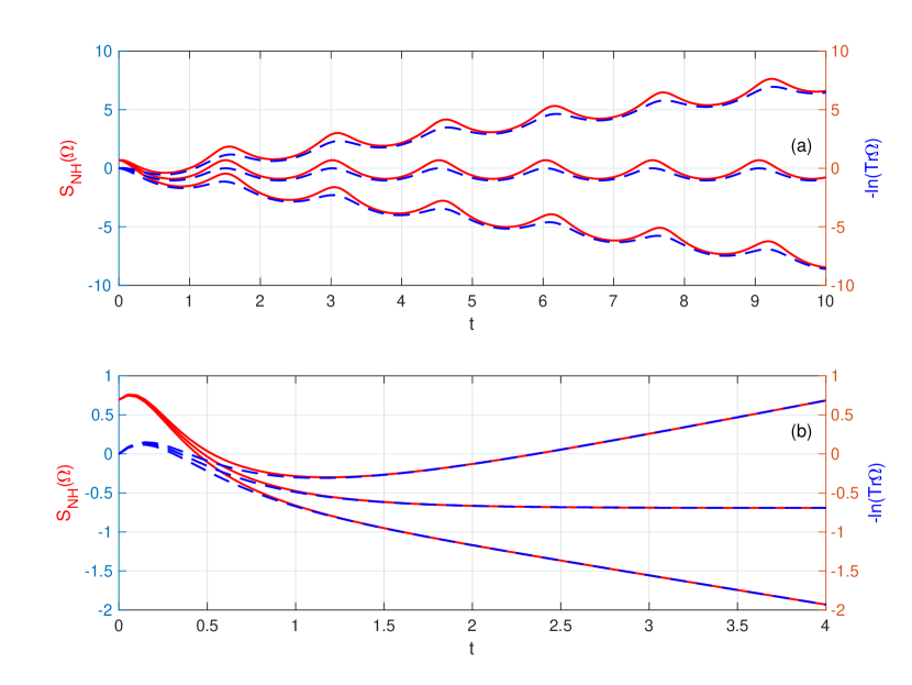
Figure 3: parameter setting: $r_{1}=2$, $\theta_{1}=\pi/6$. (a) $r=\frac{5}{\sqrt{3}}$, $\delta<0$, $H_{{\rm APT}}$ in PT symmetry broken phase, $\Delta_{{\rm APT}}$ is real. $\theta=11\pi/24,\;\pi/2,\;13\pi/24$, corresponding to $r\cos\theta>0,\;=0,\;<0$, respectively. The periodic oscillation and overall decrease (stable, increase) of $S_{{\rm NH}}$ is well predicted by Eq.(30) . (b) $\theta=2\pi/3$, $\delta>0$, $H_{{\rm APT}}$ in PT symmetry unbroken phase, $\Delta_{{\rm APT}}$ is pure imaginary. $r=2.1,\;2,\;1.9$, correspond to $\lambda>0,\;=0,\;<0$ respectively. The overall decrease (stable, increase) of $S_{{\rm NH}}$ is well predicted by Eq.(28) .

Here we discuss $S_{{\rm NH}}$ of $H_{\varphi}$ in the PT-unbroken phase, i.e., $\delta>0$. When $-\pi<\varphi<0$, Eq.(33) predicts that $S_{{\rm NH}}$ of $H_{\varphi}$ will be a combination of $S_{{\rm NH}}$ of $H_{{\rm PT}}$ and $H_{{\rm APT}}$. The decay part $e^{q\cdot 2tr\cos\theta/\hbar}$ and the oscillation part ${\rm Tr}_{{\rm PT}}^{p}$ lead to damped oscillation, a new novel phenomenon of $H_{\varphi}$. When $\varphi$ is close to 0, the oscillation is notable; when $\varphi$ gets closer to $-\pi$, oscillation becomes weaker, just as expected; we show the phenomena in fig.(4) and fig.(5). The overall decrease (stable, increase) patterns of $S_{{\rm NH}}$ depending on the value of $\lambda$ is showed in fig. 5(a), 5(b), and 5(c), which is well predicted by Eq.(34). The criticality of information flow emerges in $S_{{\rm NH}}$ of $H_{\varphi}$ too, which is showed in fig.5(d). However, the criticality gradually disappears with the damped oscillation.

Figure 4: parameter setting: $r=r_{1}=1$, $\theta_{1}=\pi/6$, $\theta=3\pi/4$; we then have $\delta>0$ and $\lambda=0$. $\lambda=0$ predicts the overall stable of $S_{{\rm NH}}$, as we show here. (a) $\varphi=-\pi/36$, (b) $\varphi=-\pi/12$, (c) $\varphi=-\pi/6$, (d) $\varphi=-3\pi/4$. Clearly, the relaxation time of the damped oscillation is determined by the value of $q\cdot 2r\cos\theta$.

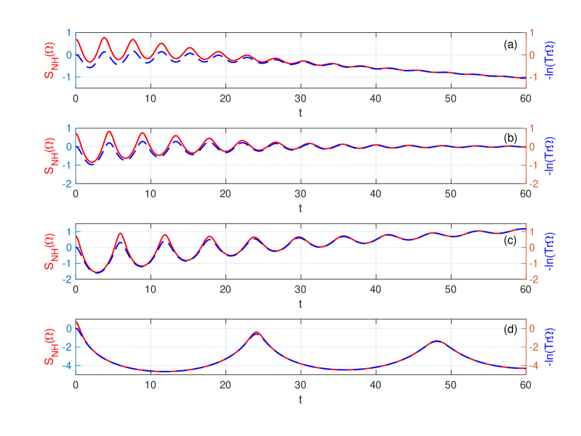
Figure 5: parameter setting: $r_{1}=1$, $\theta_{1}=\pi/6$; (a) $r=0.8$, $\varphi=-\pi/36$, $\theta=3\pi/4$, $\lambda>0$; (b) $r=1$, $\varphi=-\pi/36$, $\theta=3\pi/4$, $\lambda=0$; (c) $r=1.2$, $\varphi=-\pi/36$, $\theta=3\pi/4$, $\lambda<0$. The damped oscillation and overall decrease (stable, increase) of $S_{{\rm NH}}$ is well predicted by Eq.(34). (d) $\varphi=-\pi/48$, $r=1$, $\theta=13\pi/24$, $\lambda=0$.

Furthermore, consider a four-dimensional PT symmetric system described by the Hamiltonian [37]

$$H_{\mathcal{PT}}=-JS_{x}+\text{i}\gamma S_{z}$$ (10)

the matrix form is

$$H_{\mathcal{PT}}=\frac{1}{2}\begin{pmatrix}3\text{i}\gamma&-\sqrt{3}J&0&0\\ -\sqrt{3}J&\text{i}\gamma&-2J&0\\ 0&-2J&-\text{i}\gamma&-\sqrt{3}J\\ 0&0&-\sqrt{3}J&-3\text{i}\gamma\end{pmatrix}$$ (11)

the parity operator is $\mathcal{P}=\mathrm{antidiag}(1,1,1,1)$. The four equally spaced eigenvalues of $H_{\mathcal{PT}}$ are $\kappa_{i}=\{-3/2,-1/2,+1/2,+3/2\}\sqrt{J^{2}-\gamma^{2}}$ ($i=1,2,3,4$), with adjacent energy gap $\Delta=\sqrt{J^{2}-\gamma^{2}}$ and an exceptional point of order 4 located at $\gamma=J$ [37]. To some extent, $S_{{\rm NH}}$ of $H_{\mathcal{PT}}$ showed in fig.(6) demonstrates that our approach is effective for two-level system as well as high-dimensional system.

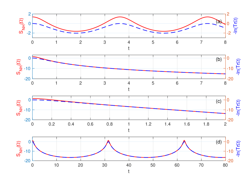
Figure 6: Setting $J=2$. (a) $\gamma=1$, $\Delta=\sqrt{3}$, PT symmetry is unbroken. (b) $\gamma=2$, $\Delta=0$, system at the exceptional point. (c) $\gamma=3$, $\Delta=\sqrt{5}i$, PT symmetry is broken. (d) $\gamma=1.99$, $\Delta=0.2$, system in the vicinity of exceptional point, criticality of information flow emerges.

IV Comparison of approaches and negative entropy

For PT symmetric systems, complete information retrieval from the environment being achieved in the PT-unbroken phase and criticality of information flow emerging around the PT exceptional point were found by characterizing information flow with the trace distance between two quantum states of a two-level system [6].

$$D\left(\rho_{1}\left(t\right),\rho_{2}\left(t\right)\right)=\frac{1}{2}\mathrm{tr}\left|\,\rho_{1}\left(t\right)-\rho_{2}\left(t\right)\,\right|$$ (12)

$$\rho_{i}=\frac{\Omega_{i}(t)}{{\rm Tr}(\Omega_{i}(t))}\quad i=1,2$$ (13)

$$\Omega_{i}(t)=e^{-\text{i}H_{{\rm PT}}t/\hbar}\Omega_{i}(0)e^{\text{i}H_{{\rm PT}}^{\dagger}t/\hbar}$$ (14)

where $|\rho|:=\sqrt{\rho^{{\dagger}}\rho}$, $\rho_{1}$ and $\rho_{2}$ are normalized density matrices. The trace distance $D$ measures the distinguishability of two quantum states since $\left[1+D\left(\rho_{1},\rho_{2}\right)\right]/2$ is the maximal probability of the two states $\rho_{1}$ and $\rho_{2}$ being successfully distinguished [57, 58, 6]. However, the normalization procedure Eq.(13) and dealing solely with the normalized density operator in [6] causes loss of information about the characterization of the open quantum system.

We compare four kinds of information dynamics: distinguishability $D$, von Neumann entropy $S_{{\rm vN}}$, $S_{{\rm NH}}$ and $-\ln{\rm Tr}(\Omega)$ of $H_{{\rm PT}}$ in fig.(7). To make the four kinds of information dynamics comparable, the initial states are chose so that they all start from their maximum value: distinguishability $D$ is maximal when the two quantum states are orthogonal, so the initial states $\Omega_{1}(0)$ and $\Omega_{2}(0)$ are set to be $|0\rangle\langle 0|$ and $|1\rangle\langle 1|$, respectively; the initial states of other three kinds of information dynamics are all set to be the maximally mixed state $\Omega(0)$. We’d like to remark that non-unitary evolution governed by non-Hermitian Hamiltonian provides, in general, a non-zero von Neumann entropy production. Apart from the periodic behavior of the four kinds of information dynamics being accordant, it’s evident that distinguishability $D$ and $S_{{\rm vN}}$ are highly correlated (the analytical expression of trace distance $D$ is easier to get) and the correlation becomes stronger as the system getting closer to exceptional point, just as $S_{{\rm NH}}$ and $-\ln{\rm Tr}(\Omega)$ are. Therefore, the four kinds of information dynamics can be divided into two groups, and the distinction between them is clearly whether or not they use the non-normalized density operator $\Omega(t)$. If we use $\frac{\partial}{\partial t}D$ or $\frac{\partial}{\partial t}S_{{\rm vN}}$ to indicate the information flow and thus to characterize the non-Markovian and Markovian processes of the systems, Fig.(7) shows that when the systems get closer to exceptional point, $\frac{\partial}{\partial t}D$ and $\frac{\partial}{\partial t}S_{{\rm vN}}$ are practically zero for most part of every period, indicating the dynamics is neither non-Markovian nor Markovian. In contrast, $S_{{\rm NH}}$ and $-\ln{\rm Tr}(\Omega)$ properly characterize the non-Markovian and Markovian processes of the systems.

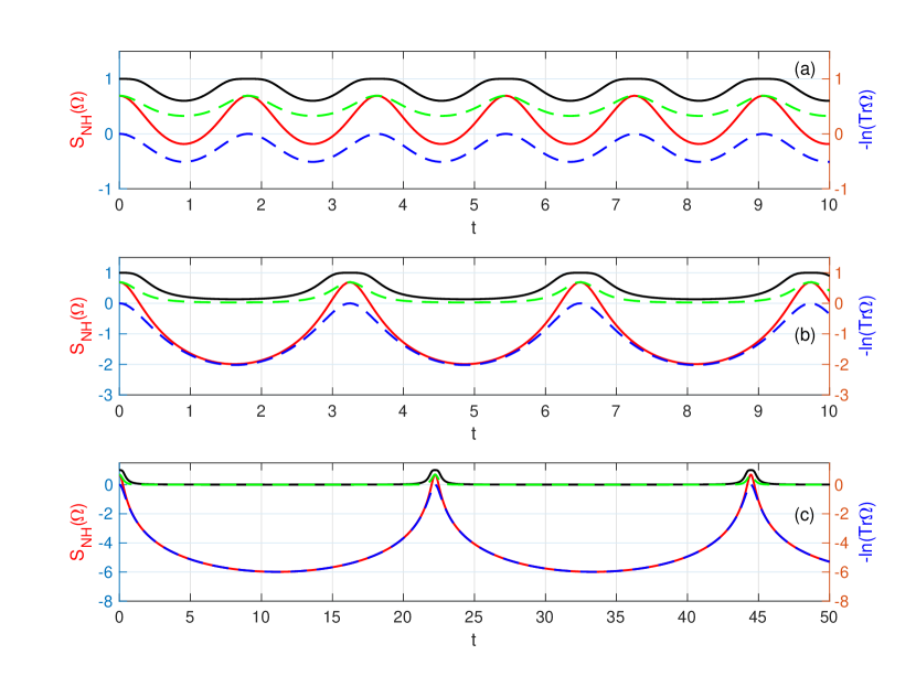
Figure 7: The black line represents distinguishability $D$, the dashed green line represents von Neumann entropy $S_{{\rm vN}}$. Parameter setting: $r_{1}=2$, $\theta_{1}=\pi/6$, $\theta=\pi/6$. (a) $r=2$, $\delta=3$; (b) $r=3.5$, $\delta=\frac{15}{16}$; (c) $r=3.99$, $\delta=0.02$, system in the vicinity of exceptional point. Compared with $S_{{\rm NH}}$ and $-\ln{\rm Tr}(\Omega)$, it seems that $D$ and $S_{{\rm vN}}$ are cut off to zero by their lower bounds and thus fail at characterizing the non-Markovian and Markovian processes of the systems properly.

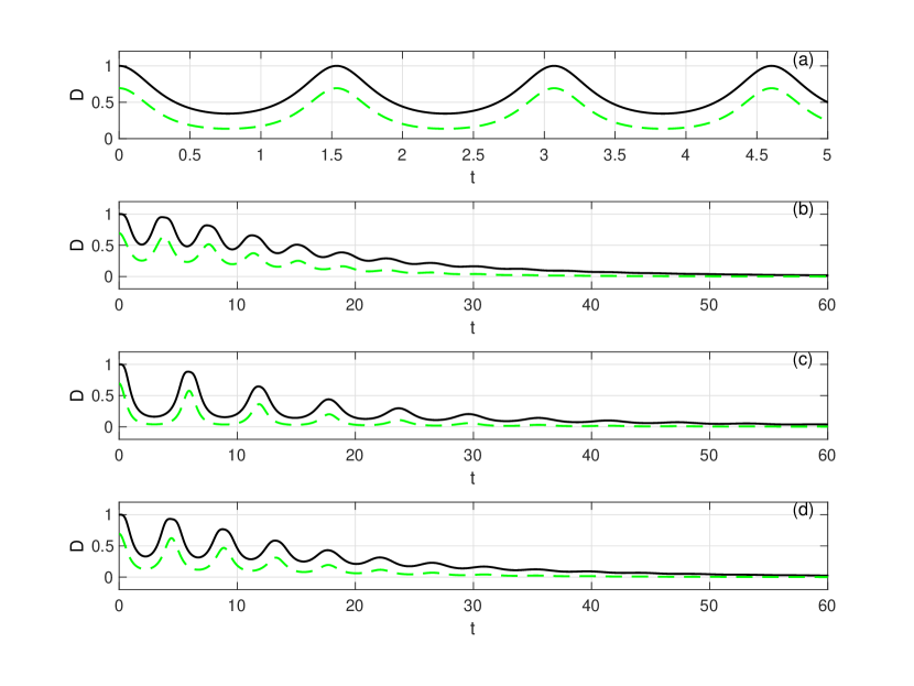
Figure 8: The black line represents distinguishability $D$, the dashed green line represents von Neumann entropy $S_{{\rm vN}}$. (a) For APT symmetric system, all parameters are same as fig.(3a) with $r\cos\theta>0$. While $S_{{\rm NH}}$ and $-\ln{\rm Tr}(\Omega)$ periodically oscillate and have an overall decrease, $D$ and $S_{{\rm vN}}$ only show the oscillation because the normalization washes out the decay part $e^{2tr\cos\theta/\hbar}$. For anyonic-PT symmetric system, (b) $\varphi=-\pi/36$, $r=0.8$, $\lambda>0$, all parameters are same as fig.(5a); (c) $\varphi=-\pi/36$, $r=1.2$, $\lambda<0$, all parameters are same as fig.(5c); (d) $\varphi=-\pi/36$, $r=1$, $\lambda=0$, all parameters are same as fig.(5b). While non-Hermitian entropy $S_{{\rm NH}}$ and $-\ln{\rm Tr}(\Omega)$ show damped oscillation with overall decrease (stable, increase), the three patterns are distorted by $D$ and $S_{{\rm vN}}$ and degenerate to the same pattern as we show here. We see that the distortion is related with the lower bounds of $D$ and $S_{{\rm vN}}$ being zero.

For $H_{{\rm APT}}$ and general $H_{\varphi}$, all the trace expressions of $H_{{\rm APT}}$ and $H_{\varphi}$ possess a decay part, $e^{2tr\cos\theta/\hbar}$ for $H_{{\rm APT}}$ and $e^{q\cdot 2tr\cos\theta}$ for $H_{\varphi}$. The decay part captures the dynamics feature of the systems and is the origin of the novel information dynamical phenomena we discussed above. For example, as we show in fig.(8), there will be no overall stable damped oscillation or periodic oscillation with overall increase or decrease if the decay part is washed out by the normalization. A simple demonstration is given in Appendix.

Here comes the problem that $S_{{\rm NH}}$ can be negative and the comparison above gives a phenomenological justification for the necessity of it. We go one step further and give a phenomenological description of the process that entropy of NH system go to negative values. Entropy measures the degree of uncertainty. In the sense of classical statistical mixture, a closed system with complete certainty is possible, and thus it’s reasonable that the lower bound of von Neumann entropy is zero, i.e., the system in a pure state. However, an general open quantum system can’t possess complete certainty since it constantly interacts with its external environment in a unpredictable way. So, if we take the entropy of closed systems as reference, it’s natural that for open quantum systems, entropy might be negative. For example, unique properties of PT symmetric systems are always predicted and observed in classical or quantum systems where gain and loss of energy or amplitude are balanced. Then, we can reasonably expect that different magnitudes of the balanced gain and loss will lead to different lower bounds of entropy, as we show in fig.(7).

Negative entropy is possible and important in Hermitian physics too. It is well known that quantum information theory has peculiar properties that cannot be found in its classical counterpart. For example, an observer’s uncertainty about a system, if measured by von Neumann conditional entropy, can become negative [38, 39, 40]. With the density matrix of the combined system of $A$ and $B$ being $\rho_{AB}$ (${\rm Tr}\rho_{AB}=1$), von Neumann conditional entropy is defined as

$$S(A|B)=-{\rm Tr}(\rho_{AB}\ln\rho_{A|B})$$ (15)

which is based on a conditional ”amplitude” operator $\rho_{A|B}$ [40]. The eigenvalues of $\rho_{A|B}$ can exceed 1 and it is precisely for this reason that the von Neumann conditional entropy can be negative [40]. For our purpose, the similarity between Eq.(15) and Eq.(8) inspires a comparison of the role of non-normalized density matrix $\Omega$ in NH entropy $S_{{\rm NH}}$ and the role of $\rho_{A|B}$ in von Neumann conditional entropy $S(A|B)$, we remark that the mathematical reason why $S_{{\rm NH}}$ can be negative is similar to $S(A|B)$, as ${\rm Tr}\,\Omega$ can exceed 1. The strong correlation between $-\ln{\rm Tr}\,\Omega$ and $S_{{\rm NH}}$ also suggests that ${\rm Tr}\,\Omega>1$ will lead to negative entropy. Negative von Neumann conditional entropy has been given a physical interpretation in terms of how much quantum communication is needed to gain complete quantum information [38]. Furthermore, a direct thermodynamical interpretation of negative conditional entropy is given in [39]. For NH entropy, our results above demonstrate that allowing NH entropy to be negative is necessary and inevitable if we want to characterize the information dynamics of NH system properly.

Conclusion and outlook. —

We have developed a new approach to characterize the information dynamics of NH systems and revealed three information-dynamics patterns in different parameter space of anyonic-PT (including APT) symmetric systems, respectively, while the approaches of the von Neumann entropy or trace distance lead to a three-fold degenerate pattern and distort it. We demonstrate that the degeneracy is caused by the normalization of the NH-evolved density matrix. Our results show that the lower bounds of both conventional entropy and trace distance being zero is related to their distortion of the information dynamics of the NH systems, and thus our work can provide a phenomenological justification for the necessity of negative NH entropy. Furthermore, we find there is a strong and comprehensible correspondence in the definition of NH entropy and quantum conditional entropy, and both quantities can be negative for similar mathematical reasons, opening up the new journey to rigorously investigate the physical interpretations of negative entropy in NH system.

Acknowledgements. —

This work was supported by the National Natural Science Foundation of China (Grant Nos. 12175002, 11705004), the Natural Science Foundation of Beijing (Grant No. 1222020), the Project of Cultivation for Young top-notch Talents of Beijing Municipal Institutions (BPHR202203034). Zhihang Liu acknowledges valuable discussions with Daili Li.

V Appendix

Trace of non-Hermitian systems

With the parity operator $\mathcal{P}$ given by $\begin{pmatrix}0&1\\ 1&0\end{pmatrix}$, and $\mathcal{T}$ being the operation of complex conjugation, in two-level system, $H_{{\rm PT}}$ can be expressed as a four-parameter family of matrices:

$$H_{{\rm PT}}=\begin{pmatrix}re^{\text{i}\theta}&r_{1}e^{\text{i}\theta_{1}}\\ r_{1}e^{-\text{i}\theta_{1}}&re^{-\text{i}\theta}\end{pmatrix},$$ (16)

with a family of corresponding $H_{{\rm APT}}$:

$$H_{{\rm APT}}=\text{i}H_{{\rm PT}}=\text{i}\begin{pmatrix}re^{\text{i}\theta}&r_{1}e^{\text{i}\theta_{1}}\\ r_{1}e^{-\text{i}\theta_{1}}&re^{-\text{i}\theta}\end{pmatrix},$$ (17)

where $r,\theta,r_{1},\theta_{1}$ are four independent real parameters. We decompose the $H_{{\rm PT}}$ in Pauli matrix.

$$H_{{\rm PT}}=r\cos\theta I+r_{1}\cos\theta_{1}\sigma_{1}-r_{1}\sin\theta_{1}\sigma_{2}+\text{i}r\sin\theta\sigma_{3}.$$ (18)

With $\text{i}r\sin\theta\sigma_{3}$ being the non-Hermitian part of $H_{{\rm PT}}$, $r\sin\theta$ represents the degree of non-Hermiticity of $H_{{\rm PT}}$. The energy eigenvalues of $H_{{\rm PT}}$ are $E_{\pm}=r\cos\theta\pm\sqrt{\delta}$ with

$$\delta=r_{1}^{2}-r^{2}\sin^{2}\theta.$$ (19)

In particular, when $r_{1}=r$, $\sqrt{\delta}=\left|r\cos\theta\right|$. For the PT symmetric system, PT symmetry is unbroken for $\delta>0$ and spontaneously broken for $\delta<0$; exceptional point is located at $\delta=0$ with the order $n=2$. The energy difference $\Delta_{{\rm PT}}$ of the two-level PT symmetric system is $\Delta_{{\rm PT}}=E_{+}-E_{-}=2\sqrt{\delta}$. The eigenvalues of $H_{{\rm APT}}$ are $E_{\pm}^{\prime}=\text{i}E_{\pm}$ and the energy difference $\Delta_{{\rm APT}}$ of the two-level APT symmetric system is $\Delta_{{\rm APT}}=\text{i}(E_{+}-E_{-})=2\text{i}\sqrt{\delta}$. For the APT symmetric system, when $\delta>0$, the system in PT symmetry unbroken phase; when $\delta<0$, the system in PT-broken phase [8]; the exceptional point of $H_{{\rm APT}}$ locates at $\delta=0$ too. When $\delta<0$, $\Delta_{{\rm APT}}$ is real, $E_{\pm}^{\prime}=\mp\sqrt{-\delta}+\text{i}r\cos\theta$, and $E_{\pm}^{\prime}$ are complex numbers if $r\cos\theta\neq 0$.

Below we set initial density matrix as a typical mixed state in two-level system, $\Omega(0)=\begin{pmatrix}\frac{1}{2}&0\\ 0&\frac{1}{2}\end{pmatrix}=\frac{1}{2}I$, which can be seen as $\frac{1}{2}|+\rangle\langle+|+\frac{1}{2}|-\rangle\langle-|$ or $\frac{1}{2}|0\rangle\langle 0|+\frac{1}{2}|1\rangle\langle 1|$. With $\Omega(0)$ being a maximally mixed state, von Neumann entropy and $S_{{\rm NH}}$ are maximal for it.

To investigate $H_{{\rm PT}}$ system, we set $\varphi=0$. When $\delta=0$, $H_{{\rm PT}}$ at the exceptional point,

$${\rm Tr}\,\Omega(t)=1+(r_{1}^{2}+r^{2}\sin^{2}\theta)(t/\hbar)^{2}.$$ (20)

For significantly large $t$,

$$-\ln{\rm Tr}\,\Omega(t)=-\ln(r_{1}^{2}+r^{2}\sin^{2}\theta)-2\ln(t/\hbar).$$ (21)

In all the expressions of trace below, we should bear in mind that we are also interested in $-\ln{\rm Tr}\,\Omega(t)$. Since logarithm is monotonic, it’s easy to understand the behavior of $-\ln{\rm Tr}\,\Omega(t)$ from the expression of ${\rm Tr}\,\Omega(t)$. And we’ll show that $-\ln{\rm Tr}\,\Omega(t)$ predicts well the behavior of $S_{{\rm NH}}$. When $\delta>0$, PT symmetry is unbroken and energy difference $\Delta_{{\rm PT}}=E_{+}-E_{-}=2\sqrt{\delta}$ is real and positive,

$${\rm Tr}\,\Omega(t)=\cos^{2}t\sqrt{\delta}/\hbar+\frac{r_{1}^{2}+r^{2}\sin^{2}\theta}{\delta}\sin^{2}t\sqrt{\delta}/\hbar.$$ (22)

Further simplification leads to

$${\rm Tr}\,\Omega(t)=\frac{1-a}{2}\cos 2\sqrt{\delta}t/\hbar+\frac{1+a}{2},$$ (23)

where $a=\frac{r_{1}^{2}+r^{2}\sin^{2}\theta}{\delta}$. It’s evident that $a\geq 1$ and ${\rm Tr}\,\Omega(t)\in\left[1,a\right]$. $a=1$ if and only if $r\sin\theta=0$, i.e., degree of non-Hermiticity of $H_{{\rm PT}}$ is zero, which is consistent with $H_{{\rm PT}}$ degenerating to a Hermitian Hamiltonian and ${\rm Tr}\,\Omega(t)$ being constant 1 when $a=1$. So, we’ll not consider the $a=1$ case. with $a>1$, Eq.(23) manifests simple harmonic dynamics, with amplitude $\left|\frac{1-a}{2}\right|$, period $T=\frac{2\pi\hbar}{2\sqrt{\delta}}=\frac{2\pi\hbar}{E_{+}-E_{-}}$. Eq.(23) and corresponding $-\ln{\rm Tr}(\Omega(t))$ periodically oscillates over time with a frequency of $\frac{E_{+}-E_{-}}{2\pi\hbar}$, which is simply the unique Bohr frequency of the PT symmetric non-Hermitian system. In standard (Hermitian) quantum mechanic, Bohr frequencies$\frac{\left|E_{n^{\prime}}-E_{n}\right|}{2\pi\hbar}$ manifesting as a intrinsic physical implication of Schrödinger equation requires Hermiticity of $H$ being a necessary condition, and thus, emergence of Bohr frequencies in non-Hermitian system cannot be taken for granted. Expanding the $\cos$ term in Eq.(23) in Taylor series, for any fixed $t$, we find that when $\delta\to 0_{+}$, that’s to say, when $H_{{\rm PT}}$ approaches to exception point from the PT-unbroken phase,

$$\lim_{\delta\to 0_{+}}\frac{1-a}{2}\cos 2\sqrt{\delta}t/\hbar+\frac{1+a}{2}=1+(r_{1}^{2}+r^{2}\sin^{2}\theta)(t/\hbar)^{2},$$ (24)

i.e., the limit of ${\rm Tr}\,\Omega(t)$ in PT symmetry unbroken phase as $\delta\to 0_{+}$ is exactly ${\rm Tr}\,\Omega(t)$ at exception point. We’ll show that Eq.(21) and Eq.(24) can explain the information criticality phenomenon in the non-Hermitian entropy dynamics. When $\delta<0$, PT symmetry is spontaneously broken, the eigenvalues are complex conjugation pair, and energy difference $\Delta_{{\rm PT}}=E_{+}-E_{-}=2\sqrt{\delta}$ is a pure imaginary number.

$${\rm Tr}\,\Omega(t)=\frac{1+b}{2}\cosh 2\sqrt{-\delta}t/\hbar+\frac{1-b}{2},$$ (25)

where $b=\frac{r_{1}^{2}+r^{2}\sin^{2}\theta}{-\delta}$, $b\geq 1$, $b=1$ if and only if $r_{1}=0$.

To investigate $H_{{\rm APT}}$ system, we set $\varphi=-\pi$. When $\delta=0$,

$${\rm Tr}\,\Omega(t)=e^{2tr\cos\theta/\hbar}(1+(r_{1}^{2}+r^{2}\sin^{2}\theta)(t/\hbar)^{2}).$$ (26)

When $\delta>0$, energy difference $\Delta_{{\rm APT}}=i(E_{+}-E_{-})=2i\sqrt{\delta}$ is a pure imaginary number,

$${\rm Tr}\,\Omega(t)=e^{2tr\cos\theta/\hbar}(\frac{1+a}{2}\cosh 2\sqrt{\delta}t/\hbar+\frac{1-a}{2}),$$ (27)

where $a=\frac{r_{1}^{2}+r^{2}\sin^{2}\theta}{\delta}$, $a\geq 1$. It’s evident that $\frac{1+a}{2}\cosh 2\sqrt{\delta}t/\hbar+\frac{1-a}{2}\geq 1$ and ${\rm Tr}\,\Omega(t)>0$. The asymptotic behavior of Eq.(27) depends on values of the parameters. When $t$ is significantly large,

$${\rm Tr}\,\Omega(t)\approx\frac{1+a}{4}e^{2\lambda t/\hbar},$$ (28)

with

$$\lambda=r\cos\theta+\sqrt{\delta}.$$ (29)

In particular, $\lambda=0$ if and only if $\left|r_{1}\right|=\left|r\right|$ and $r\cos\theta<0$. When $\delta<0$, energy difference $\Delta_{{\rm APT}}=2i\sqrt{\delta}$ is a real number,

$${\rm Tr}\,\Omega(t)=e^{2tr\cos\theta/\hbar}(\frac{1-b}{2}\cos(2\sqrt{-\delta}t/\hbar)+\frac{1+b}{2}),$$ (30)

where $b=\frac{r_{1}^{2}+r^{2}\sin^{2}\theta}{-\delta}\geq 1$. If we neglect the constant $\frac{1+b}{2}$, Eq.(30) is the equation of underdamped oscillation, with the undamped frequency $\omega^{2}=4(r^{2}-r_{1}^{2})$. For $H_{{\rm APT}}$, similar to Eq.(24), it’s easy to know that the limit of Eq.(30) as $\delta\to 0_{-}$ is exactly ${\rm Tr}\,\Omega(t)$ at exception point. Comparing trace expressions of $H_{{\rm PT}}$ and $H_{{\rm APT}}$, the first difference is the decay term $e^{2tr\cos\theta/\hbar}$; When $r\cos\theta=0$, the first difference disappears. Therefore, in order to study the unique properties of $H_{{\rm APT}}$ with respect to $H_{{\rm PT}}$, it’s better to investigate $H_{{\rm APT}}$ for which $r\cos\theta\neq 0$. The second difference is that periodicity emerges in PT-unbroken phase for $H_{{\rm PT}}$ and in PT-broken phase for $H_{{\rm APT}}$. It’s notable that, for $H_{{\rm PT}}$ or $H_{{\rm APT}}$, periodicity emerges only when energy difference is real.

For anyonic-PT symmetric system, we give a detailed analysis for the system in PT-unbroken phase, i.e., when $\delta>0$ (the analysis for the system in PT-broken phase or at exceptional point can be done in a similar way). With $e^{-\text{i}\frac{\varphi}{2}}=p+\text{i}q$, $p=\cos\frac{\varphi}{2},q=-\sin\frac{\varphi}{2}$, we then have

$$H_{\varphi}=e^{-\text{i}\frac{\varphi}{2}}H_{{\rm PT}}=pH_{{\rm PT}}+q(\text{i}H_{{\rm PT}}),$$ (31)

and notice that $\text{i}H_{{\rm PT}}$ satisfies APT symmetry. We then have

$$\begin{aligned} {\rm Tr}\,\Omega(t)&=\frac{1-a}{2}e^{q\cdot 2tr\cos\theta/\hbar}\cos(2p\sqrt{\delta}t/\hbar)+\frac{1+a}{2}e^{q\cdot 2tr\cos\theta/\hbar}\cos(2\text{i}q\sqrt{\delta}t/\hbar)\\ &={\rm Tr}^{{\rm re}}+{\rm Tr}^{{\rm im}}\end{aligned},$$ (32)

where ${\rm Tr}^{{\rm re}}=\frac{1-a}{2}e^{q\cdot 2tr\cos\theta/\hbar}\cos(2p\sqrt{\delta}t/\hbar)$, ${\rm Tr}^{{\rm im}}=\frac{1+a}{2}e^{q\cdot 2tr\cos\theta/\hbar}\cos(2\text{i}q\sqrt{\delta}t/\hbar)$.

When $q\cdot 2r\cos\theta<0$, ${\rm Tr}^{{\rm re}}$ is the equation of underdamped oscillation, with the undamped frequency $\omega^{2}=4(p^{2}\delta+q^{2}r^{2}\cos^{2}\theta)$, in particular, when $\left|r\right|=\left|r_{1}\right|$, $\delta=r^{2}\cos^{2}\theta$, $\omega^{2}=4r^{2}\cos^{2}\theta$. ${\rm Tr}^{{\rm im}}$ is the equation of overdamped oscillation, with the undamped frequency $\omega^{2}=4q^{2}(r^{2}-r_{1}^{2})$, in particular, when $\left|r\right|=\left|r_{1}\right|$, $\omega^{2}=0$. So, Eq.(32) is a combination of the underdamped oscillation and the overdamped oscillation; when $\left|r\right|=\left|r_{1}\right|$, the undamped frequencies are independent of $\varphi$. Especially, when $a=1$, $r\sin\theta=0$ ($H_{\varphi}$ is still non-Hermitian), ${\rm Tr}^{{\rm re}}=0$, Eq.(32) becomes the equation of overdamped oscillation. When $q\cdot 2r\cos\theta>0$, corresponding amplified oscillations can be analyzed in the same way. Rewrite Eq.(32) as

$$\begin{aligned} {\rm Tr}\,\Omega(t)&=e^{q\cdot 2tr\cos\theta/\hbar}\left[(\frac{1-a}{2}\cos(p\cdot 2\sqrt{\delta}t/\hbar)+\frac{1+a}{2})+(\frac{1+a}{2}\cosh(q\cdot 2\sqrt{\delta}t/\hbar)+\frac{1-a}{2})-1\right]\\ &=e^{q\cdot 2tr\cos\theta/\hbar}({\rm Tr}_{{\rm PT}}^{p}+{\rm Tr}_{{\rm APT}}^{q}-1)\end{aligned},$$ (33)

where ${\rm Tr}_{{\rm PT}}^{p}=\frac{1-a}{2}\cos(p\cdot 2\sqrt{\delta}t/\hbar)+\frac{1+a}{2}$, ${\rm Tr}_{{\rm APT}}^{q}=\frac{1+a}{2}\cosh(q\cdot 2\sqrt{\delta}t/\hbar)+\frac{1-a}{2}$.

Compared to Eq.(23) and Eq.(27), ${\rm Tr}_{{\rm PT}}^{p}$ is reminiscent of the trace expression of $H_{{\rm PT}}$ in PT-unbroken phase and ${\rm Tr}_{{\rm APT}}^{q}$ is reminiscent of the trace of $H_{{\rm APT}}$ in PT-unbroken phase. When $\varphi=0$, we restore Eq.(23); when $\varphi=-\pi$, we restore Eq.(27). It’s notable that $\theta_{1}$ plays no role in all the trace expressions, which shows a robustness against parameter change. For $H_{\varphi_{1}}$ and $H_{\varphi_{2}}$ with $\varphi_{1}+\varphi_{2}=-2\pi$ or $2\pi$, the trace expressions of $H_{\varphi_{1}}$ and $H_{\varphi_{2}}$ are same. For significantly large $t$, ${\rm Tr}_{{\rm APT}}^{q}$ is the dominator of Eq.(33), and we have

$${\rm Tr}\,\Omega(t)\approx\frac{1+a}{4}e^{2q\lambda t/\hbar}$$ (34)

Eq.(34) determines the overall trend of Eq.(33), with $\lambda=r\cos\theta+\sqrt{\delta}$ ($\lambda=0$ if and only if $\left|r_{1}\right|=\left|r\right|$ and $r\cos\theta<0$ ). It’s evident that Eq.(28) is a special case of Eq.(34) for $\varphi=-\pi$.

Derivation of Eq.(33)

Decompose the $H_{{\rm PT}}$ in Pauli matrix,

$$H_{{\rm PT}}=r\cos\theta I+r_{1}\cos\theta_{1}\sigma_{1}-r_{1}\sin\theta_{1}\sigma_{2}+\text{i}r\sin\theta\sigma_{3},$$

and define

$$M=r_{1}\cos\theta_{1}\sigma_{1}-r_{1}\sin\theta_{1}\sigma_{2}+\text{i}r\sin\theta\sigma_{3}=\begin{pmatrix}\text{i}r\sin\theta&r_{1}e^{\text{i}\theta_{1}}\\ r_{1}e^{-\text{i}\theta_{1}}&-\text{i}r\sin\theta\end{pmatrix}.$$ (A.1)

With $\delta=r_{1}^{2}-r^{2}\sin^{2}\theta$, it is easy to verify that

$$M^{2}=\delta I.$$ (A.2)

The time-evolution operator $U_{\varphi}$ of the anyonic-PT symmetric system is

$$\begin{aligned} U_{\varphi}&=e^{-\text{i}tH_{\varphi}/\hbar}\\ &=e^{-\text{i}te^{-\text{i}\frac{\varphi}{2}}r\cos\theta/\hbar}\cdot(\sum_{k=0}^{\infty}\frac{(-\text{i}te^{-i\frac{\varphi}{2}}/\hbar)^{2k}\cdot M^{2k}}{2k!}+\sum_{k=0}^{\infty}\frac{(-\text{i}te^{-i\frac{\varphi}{2}}/\hbar)^{2k+1}\cdot M^{2k+1}}{(2k+1)!})\\ \end{aligned}.$$ (A.3)

When $\delta=0$, $M^{2}=\delta I=0$, we have

$$U_{\varphi}=e^{-\text{i}te^{-\text{i}\frac{\varphi}{2}}r\cos\theta/\hbar}\cdot(-\text{i}te^{-\text{i}\frac{\varphi}{2}}M/\hbar+I).$$ (A.4)

When $\delta\neq 0$,

$$\begin{aligned} U_{\varphi}&=e^{-\text{i}te^{-\text{i}\frac{\varphi}{2}}r\cos\theta/\hbar}\cdot(\sum_{k=0}^{\infty}\frac{(-\text{i}te^{-\text{i}\frac{\varphi}{2}}/\hbar)^{2k}\cdot(\sqrt{\delta})^{2k}I}{2k!}+\sum_{k=0}^{\infty}\frac{(-\text{i}te^{-\text{i}\frac{\varphi}{2}}/\hbar)^{2k+1}\cdot(\sqrt{\delta})^{2k+1}\frac{M}{\sqrt{\delta}}}{(2k+1)!})\\ &=e^{-\text{i}te^{-\text{i}\frac{\varphi}{2}}r\cos\theta/\hbar}\cdot(\cos(te^{-\text{i}\frac{\varphi}{2}}\sqrt{\delta}/\hbar)I-\text{i}\frac{\sin(te^{-\text{i}\frac{\varphi}{2}}\sqrt{\delta}/\hbar)}{\sqrt{\delta}}M)\end{aligned}.$$ (A.5)

Denote $M_{1}=\cos(te^{-\text{i}\frac{\varphi}{2}}\sqrt{\delta}/\hbar)I-\text{i}\frac{\sin(te^{-\text{i}\frac{\varphi}{2}}\sqrt{\delta}/\hbar)}{\sqrt{\delta}}M$, with $\Omega(0)=\frac{1}{2}I$, $\Omega(t)=U_{\varphi}\Omega(0)U_{\varphi}^{\dagger}$, $e^{-\text{i}\frac{\varphi}{2}}=p+\text{i}q$, $q=-\sin\frac{\varphi}{2}$. We then have

$$\Omega(t)=\frac{1}{2}e^{q\cdot 2tr\cos\theta/\hbar}\cdot M_{1}M_{1}^{\dagger}.$$ (A.6)

When $\delta>0$, with $a=\frac{r_{1}^{2}+r^{2}\sin^{2}\theta}{\delta}\geq 1$, we get Eq.(33),

$$\begin{aligned} {\rm Tr}\,\Omega(t)&=e^{q\cdot 2tr\cos\theta/\hbar}\left[(\frac{1-a}{2}\cos(2p\sqrt{\delta}t/\hbar)+\frac{1+a}{2})+(\frac{1+a}{2}\cosh(2q\sqrt{\delta}t/\hbar)+\frac{1-a}{2})-1\right]\\ &=e^{q\cdot 2tr\cos\theta}({\rm Tr}_{{\rm PT}}^{p}+{\rm Tr}_{{\rm APT}}^{q}-1)\end{aligned}.$$

When $\delta<0$, with $b=\frac{r_{1}^{2}+r^{2}\sin^{2}\theta}{-\delta}\geq 1$, we have

$$\begin{aligned} {\rm Tr}\,\Omega(t)&=e^{q\cdot 2tr\cos\theta/\hbar}\left[(\frac{1+b}{2}\cosh 2p\sqrt{-\delta}t/\hbar+\frac{1-b}{2})+(\frac{1-b}{2}\cos(2q\sqrt{-\delta}t/\hbar)+\frac{1+b}{2})-1\right]\\ &=e^{q\cdot 2tr\cos\theta/\hbar}\cdot\frac{1+b}{2}\cosh 2p\sqrt{-\delta}t/\hbar+e^{q\cdot 2tr\cos\theta/\hbar}\cdot\frac{1-b}{2}\cos(2q\sqrt{-\delta}t/\hbar)\end{aligned}.$$ (A.7)

So, similar to Eq.(32), Eq.(A.7) is a combination of underdamped oscillation and overdamped oscillation. All the trace expressions can be derived in the same way.

Consequence of the normalization procedure

The normalization procedure washes out the decay part $e^{q\cdot 2tr\cos\theta}$ ($q=1$ for $H_{{\rm APT}}$, $q=0$ for $H_{{\rm PT}}$).

$$\begin{aligned} \rho(t)&=\frac{\Omega(t)}{{\rm Tr}\,\Omega(t)}\\ &=\frac{\frac{1}{2}M_{1}M_{1}^{\dagger}}{{\rm Tr}_{{\rm PT}}^{p}+{\rm Tr}_{{\rm APT}}^{q}-1}\end{aligned}.$$ (A.8)

References

- Breuer and Petruccione [2002] Heinz-Peter Breuer and Francesco Petruccione. The theory of open quantum systems. Oxford University Press, USA, 2002.
- Barreiro et al. [2011] Julio T Barreiro, Markus Müller, Philipp Schindler, Daniel Nigg, Thomas Monz, Michael Chwalla, Markus Hennrich, Christian F Roos, Peter Zoller, and Rainer Blatt. An open-system quantum simulator with trapped ions. Nature, 470(7335):486–491, 2011.
- Hu et al. [2020] Zixuan Hu, Rongxin Xia, and Sabre Kais. A quantum algorithm for evolving open quantum dynamics on quantum computing devices. Scientific reports, 10(1):3301, 2020.
- Del Re et al. [2020] Lorenzo Del Re, Brian Rost, AF Kemper, and JK Freericks. Driven-dissipative quantum mechanics on a lattice: Simulating a fermionic reservoir on a quantum computer. Physical Review B, 102(12):125112, 2020.
- Bender and Boettcher [1998] Carl M Bender and Stefan Boettcher. Real spectra in non-hermitian hamiltonians having p t symmetry. Physical review letters, 80(24):5243, 1998.
- Kawabata et al. [2017] Kohei Kawabata, Yuto Ashida, and Masahito Ueda. Information retrieval and criticality in parity-time-symmetric systems. Physical review letters, 119(19):190401, 2017.
- Zheng et al. [2013] Chao Zheng, Liang Hao, and Gui Lu Long. Observation of a fast evolution in a parity-time-symmetric system. Philosophical Transactions of the Royal Society A: Mathematical, Physical and Engineering Sciences, 371(1989):20120053, 2013.
- Yang et al. [2017] Fan Yang, Yong-Chun Liu, and Li You. Anti-pt symmetry in dissipatively coupled optical systems. Physical Review A, 96(5):053845, 2017.
- Li et al. [2019a] Ying Li, Yu-Gui Peng, Lei Han, Mohammad-Ali Miri, Wei Li, Meng Xiao, Xue-Feng Zhu, Jianlin Zhao, Andrea Alù, Shanhui Fan, et al. Anti–parity-time symmetry in diffusive systems. Science, 364(6436):170–173, 2019a.
- Peng et al. [2016] Peng Peng, Wanxia Cao, Ce Shen, Weizhi Qu, Jianming Wen, Liang Jiang, and Yanhong Xiao. Anti-parity–time symmetry with flying atoms. Nature Physics, 12(12):1139–1145, 2016.
- Bergman et al. [2021] Arik Bergman, Robert Duggan, Kavita Sharma, Moshe Tur, Avi Zadok, and Andrea Alù. Observation of anti-parity-time-symmetry, phase transitions and exceptional points in an optical fibre. Nature Communications, 12(1):486, 2021.
- Yang et al. [2020] Ying Yang, Yi-Pu Wang, JW Rao, YS Gui, BM Yao, W Lu, and C-M Hu. Unconventional singularity in anti-parity-time symmetric cavity magnonics. Physical Review Letters, 125(14):147202, 2020.
- Choi et al. [2018] Youngsun Choi, Choloong Hahn, Jae Woong Yoon, and Seok Ho Song. Observation of an anti-pt-symmetric exceptional point and energy-difference conserving dynamics in electrical circuit resonators. Nature communications, 9(1):2182, 2018.
- Zheng [2019] Chao Zheng. Duality quantum simulation of a generalized anti-pt-symmetric two-level system. Europhysics Letters, 126(3):30005, 2019.
- Wen et al. [2020] Jingwei Wen, Guoqing Qin, Chao Zheng, Shijie Wei, Xiangyu Kong, Tao Xin, and Guilu Long. Observation of information flow in the anti-pt-symmetric system with nuclear spins. npj Quantum Information, 6(1):28, 2020.
- Mostafazadeh [2002a] Ali Mostafazadeh. Pseudo-hermiticity versus pt symmetry: the necessary condition for the reality of the spectrum of a non-hermitian hamiltonian. Journal of Mathematical Physics, 43(1):205–214, 2002a.
- Mostafazadeh [2004] Ali Mostafazadeh. Pseudounitary operators and pseudounitary quantum dynamics. Journal of mathematical physics, 45(3):932–946, 2004.
- Zheng [2022] Chao Zheng. Quantum simulation of pt-arbitrary-phase–symmetric systems. Europhysics Letters, 136(3):30002, 2022.
- Longhi and Pinotti [2019] S Longhi and E Pinotti. Anyonic symmetry, drifting potentials and non-hermitian delocalization. Europhysics Letters, 125(1):10006, 2019.
- Arwas et al. [2022] Geva Arwas, Sagie Gadasi, Igor Gershenzon, Asher Friesem, Nir Davidson, and Oren Raz. Anyonic-parity-time symmetry in complex-coupled lasers. Science advances, 8(22):eabm7454, 2022.
- Chen et al. [2014] Shin-Liang Chen, Guang-Yin Chen, and Yueh-Nan Chen. Increase of entanglement by local pt-symmetric operations. Physical review A, 90(5):054301, 2014.
- Lee et al. [2014] Tony E Lee, Florentin Reiter, and Nimrod Moiseyev. Entanglement and spin squeezing in non-hermitian phase transitions. Physical review letters, 113(25):250401, 2014.
- Couvreur et al. [2017] Romain Couvreur, Jesper Lykke Jacobsen, and Hubert Saleur. Entanglement in nonunitary quantum critical spin chains. Physical review letters, 119(4):040601, 2017.
- Ashida et al. [2017] Yuto Ashida, Shunsuke Furukawa, and Masahito Ueda. Parity-time-symmetric quantum critical phenomena. Nature communications, 8(1):15791, 2017.
- Ashida et al. [2020] Yuto Ashida, Zongping Gong, and Masahito Ueda. Non-hermitian physics. Advances in Physics, 69(3):249–435, 2020.
- Li et al. [2019b] Jiaming Li, Andrew K Harter, Ji Liu, Leonardo de Melo, Yogesh N Joglekar, and Le Luo. Observation of parity-time symmetry breaking transitions in a dissipative floquet system of ultracold atoms. Nature communications, 10(1):855, 2019b.
- Wang et al. [2022] J Wang, D Mukhopadhyay, and GS Agarwal. Quantum fisher information perspective on sensing in anti-pt symmetric systems. Physical Review Research, 4(1):013131, 2022.
- Wu et al. [2014] Jin-Hui Wu, Maurizio Artoni, and GC La Rocca. Non-hermitian degeneracies and unidirectional reflectionless atomic lattices. Physical review letters, 113(12):123004, 2014.
- Lin et al. [2011] Zin Lin, Hamidreza Ramezani, Toni Eichelkraut, Tsampikos Kottos, Hui Cao, and Demetrios N Christodoulides. Unidirectional invisibility induced by p t-symmetric periodic structures. Physical Review Letters, 106(21):213901, 2011.
- Regensburger et al. [2012] Alois Regensburger, Christoph Bersch, Mohammad-Ali Miri, Georgy Onishchukov, Demetrios N Christodoulides, and Ulf Peschel. Parity–time synthetic photonic lattices. Nature, 488(7410):167–171, 2012.
- Pechukas [1994] Philip Pechukas. Reduced dynamics need not be completely positive. Physical review letters, 73(8):1060, 1994.
- Von Neumann [2018] John Von Neumann. Mathematical foundations of quantum mechanics: New edition, volume 53. Princeton university press, 2018.
- Rényi [1961] Alfréd Rényi. On measures of entropy and information. In Proceedings of the Fourth Berkeley Symposium on Mathematical Statistics and Probability, Volume 1: Contributions to the Theory of Statistics, volume 4, pages 547–562. University of California Press, 1961.
- Li and Zheng [2022] Daili Li and Chao Zheng. Non-hermitian generalization of rényi entropy. Entropy, 24(11):1563, 2022.
- Nielsen and Chuang [2010] Michael A Nielsen and Isaac L Chuang. Quantum computation and quantum information. Cambridge university press, 2010.
- Xiao et al. [2019] Lei Xiao, Kunkun Wang, Xiang Zhan, Zhihao Bian, Kohei Kawabata, Masahito Ueda, Wei Yi, and Peng Xue. Observation of critical phenomena in parity-time-symmetric quantum dynamics. Physical Review Letters, 123(23):230401, 2019.
- Bian et al. [2020] Zhihao Bian, Lei Xiao, Kunkun Wang, Franck Assogba Onanga, Frantisek Ruzicka, Wei Yi, Yogesh N Joglekar, and Peng Xue. Quantum information dynamics in a high-dimensional parity-time-symmetric system. Physical Review A, 102(3):030201, 2020.
- Horodecki et al. [2005] Michał Horodecki, Jonathan Oppenheim, and Andreas Winter. Partial quantum information. Nature, 436(7051):673–676, 2005.
- Rio et al. [2011] Lídia del Rio, Johan Åberg, Renato Renner, Oscar Dahlsten, and Vlatko Vedral. The thermodynamic meaning of negative entropy. Nature, 474(7349):61–63, 2011.
- Cerf and Adami [1997] Nicolas J Cerf and Chris Adami. Negative entropy and information in quantum mechanics. Physical Review Letters, 79(26):5194, 1997.
- Bocchieri and Loinger [1957] P Bocchieri and A Loinger. Quantum recurrence theorem. Physical Review, 107(2):337, 1957.
- Mostafazadeh [2002b] Ali Mostafazadeh. Pseudo-hermiticity versus pt-symmetry. ii. a complete characterization of non-hermitian hamiltonians with a real spectrum. Journal of Mathematical Physics, 43(5):2814–2816, 2002b.
- Wu et al. [2019] Yang Wu, Wenquan Liu, Jianpei Geng, Xingrui Song, Xiangyu Ye, Chang-Kui Duan, Xing Rong, and Jiangfeng Du. Observation of parity-time symmetry breaking in a single-spin system. Science, 364(6443):878–880, 2019.
- Brody [2016] Dorje C Brody. Consistency of pt-symmetric quantum mechanics. Journal of Physics A: Mathematical and Theoretical, 49(10):10LT03, 2016.
- Brody and Graefe [2012] Dorje C Brody and Eva-Maria Graefe. Mixed-state evolution in the presence of gain and loss. Physical review letters, 109(23):230405, 2012.
- Brody [2013] Dorje C Brody. Biorthogonal quantum mechanics. Journal of Physics A: Mathematical and Theoretical, 47(3):035305, 2013.
- Sergi and Zloshchastiev [2016] Alessandro Sergi and Konstantin G Zloshchastiev. Quantum entropy of systems described by non-hermitian hamiltonians. Journal of Statistical Mechanics: Theory and Experiment, 2016(3):033102, 2016.
- Erez et al. [2008] Noam Erez, Goren Gordon, Mathias Nest, and Gershon Kurizki. Thermodynamic control by frequent quantum measurements. Nature, 452(7188):724–727, 2008.
- Wolf et al. [2008] Michael Marc Wolf, J Eisert, Toby S Cubitt, and J Ignacio Cirac. Assessing non-markovian quantum dynamics. Physical review letters, 101(15):150402, 2008.
- Breuer et al. [2009] Heinz-Peter Breuer, Elsi-Mari Laine, and Jyrki Piilo. Measure for the degree of non-markovian behavior of quantum processes in open systems. Physical review letters, 103(21):210401, 2009.
- Laine et al. [2010] Elsi-Mari Laine, Jyrki Piilo, and Heinz-Peter Breuer. Measure for the non-markovianity of quantum processes. Physical Review A, 81(6):062115, 2010.
- Rivas et al. [2010] Ángel Rivas, Susana F Huelga, and Martin B Plenio. Entanglement and non-markovianity of quantum evolutions. Physical review letters, 105(5):050403, 2010.
- Luo et al. [2012] Shunlong Luo, Shuangshuang Fu, and Hongting Song. Quantifying non-markovianity via correlations. Physical Review A, 86(4):044101, 2012.
- Chruściński and Maniscalco [2014] Dariusz Chruściński and Sabrina Maniscalco. Degree of non-markovianity of quantum evolution. Physical review letters, 112(12):120404, 2014.
- Chruściński et al. [2017] Dariusz Chruściński, Chiara Macchiavello, and Sabrina Maniscalco. Detecting non-markovianity of quantum evolution via spectra of dynamical maps. Physical review letters, 118(8):080404, 2017.
- Breuer et al. [2016] Heinz-Peter Breuer, Elsi-Mari Laine, Jyrki Piilo, and Bassano Vacchini. Colloquium: Non-markovian dynamics in open quantum systems. Reviews of Modern Physics, 88(2):021002, 2016.
- Fuchs and Van De Graaf [1999] Christopher A Fuchs and Jeroen Van De Graaf. Cryptographic distinguishability measures for quantum-mechanical states. IEEE Transactions on Information Theory, 45(4):1216–1227, 1999.
- Gilchrist et al. [2005] Alexei Gilchrist, Nathan K Langford, and Michael A Nielsen. Distance measures to compare real and ideal quantum processes. Physical Review A, 71(6):062310, 2005.