Multi-Target Two-way Integrated Sensing and Communications with Full Duplex MIMO Radios

Abstract

In this paper, we propose a multiple input multiple output (MIMO) Full-Duplex Integrated Sensing and Communication System consisting of multiple targets, a single downlink, and a single uplink user. We employed signal-to-interference plus noise ratio (SINR) as the performance metric for radar, downlink, and uplink communication. We use a communication-centric approach in which communication waveform is used for both communication and sensing of the environment. We develop a sensing algorithm capable of estimating direction of arrival (DoA), range, and velocity of each target. We also propose a joint optimization framework for designing A/D transmit and receive beamformers to improve radar, downlink, and uplink SINRs while minimizing self-interference (SI) leakage. We also propose a null space projection (NSP) based approach to improve the uplink rate. Our simulation results, considering Orthogonal Frequency Division Multiplexing (OFDM) waveform, show accurate radar parameter estimation with improved downlink and uplink rate.

I Introduction

The ongoing discussions for the next generation of wireless networks pronounce the role of sensing, both as a means to effectively optimize spectral and energy efficiencies, as well as a core prerequisite characteristic of future immersive applications [1]. In addition, sensing is envisioned to be offered in an integrated manner with next-generation communication services, giving birth to Integrated Sensing and Communications (ISAC) systems [2] that need to be supported by tailor-made physical-layer technologies [3, 4]. Among those technologies belong the in-band Full-Duplex MIMO systems [5], which are capable of implementing simultaneous transmission and reception operations in the same frequency band.

Prior Works. Leveraging an FD MIMO system architecture with reduced complexity analog cancellation of the SI signal[6], the authors in [7] jointly designed the base station (BS) transmit and receive beamforming (BF) matrices, as well as the settings for the multiple analog SI cancellation taps and the digital Self-Interference (SI) canceller, to maximize the downlink (DL) rate simultaneously with the optimization of the uplink (UL) channel estimation process. FD MIMO radios have been also leveraged for efficient low-latency beam management in millimeter-Wave (mmWave) systems. A multi-beam mmWave FD ISAC system was presented in [8], according to which the transmitter (TX) and receiver (RX) beamformers were optimized to have multiple beams for both communications and monostatic sensing. In [9], the RX spatial signal was further used to estimate the range and angle profiles corresponding to the multiple targets. An ISAC system, where a massive MIMO BS equipped with Hybrid analog and digital Beamforming (HBF) is communicating with multiple DL users and simultaneously estimates via the same signaling waveforms the DoA as well as the range of radar targets, has been presented in [10]. A more involved joint optimization framework for designing the analog and digital TX and RX beamformers, as well as the active analog and digital SI cancellation units, was presented in [11] with the objective to maximize the achievable DL rate and the accuracy performance of the DoA, range, as well as the relative velocity estimation of radar targets. In [12], a BF optimization framework to maximize radar sensing and the DL users gain patterns while eradicating the SI leakage power through a NSP method, was presented. Moreover, in [13] different TX precoding techniques have been discussed for dual-function radar-communication (DFRC) systems to ensure radar and communication guarantees. Very recently, in [14], an FD MIMO architecture incorporating metasurface-based holographic MIMO transceivers [15] was optimized for near-field ISAC in sub-THz frequencies. In [16], a reconfigurable intelligent surface was deployed in the near-field region of an FD MIMO node and was jointly optimized with the MIMO digital BF to enable simultaneous communications and sensing of passive objects, while efficiently handling SI.

Contributions. In this paper, we consider an Full Duplex Integrated Sensing and Communication (FD-ISAC) system consisting of multiple radar targets, single DL and single UL communication user. Unlike the previous work in [11], where a sub-optimal TX precoding was presented because of bad performance at high TX signal to noise ratio (SNR) regime, we present an optimal approach using the Lagrangian duality method and derive the solution for the case of a single RX RF chain. Moreover, to increase the UL rate, we propose an NSP-based approach to mitigate the radar interference from the intended UL user signal. A similar problem was investigated in [17], however, only digital BF was considered at the BS and user, which is rather intractable for large antenna arrays. The presented numerical results showcase that the proposed FD-ISAC scheme performs sufficiently well in terms of radar as well as DL and UL SINRs, while suppressing the SI power to a desired threshold.

The remainder of the paper is organized as follows: Section II describes the system model. Section III presents the sensing parameters estimation procedure (DoA, range and velocity of each target). In Section IV optimization framework is provided to optimize the beamformer to increase the corresponding SINRs. In Section V numerical results are provided and finally, Section VI concludes the paper.

Notations: Matrices are denoted in uppercase bold letters (i.e., $\mathbf{H}$) while vectors in lowercase bold letters (i.e., $\mathbf{w}$). Sets of real and complex numbers are represented by $\mathbb{R}$ and $\mathbb{C}$ respectively. $||.||_{\text{F}}$ represents the Frobenius norm and $||.||_{2}$ represents the $\ell-2$ norm. $[\mathbf{A}]_{(i,:)}$ represents the $i$-th row of matrix $\mathbf{A}$.

II System Model

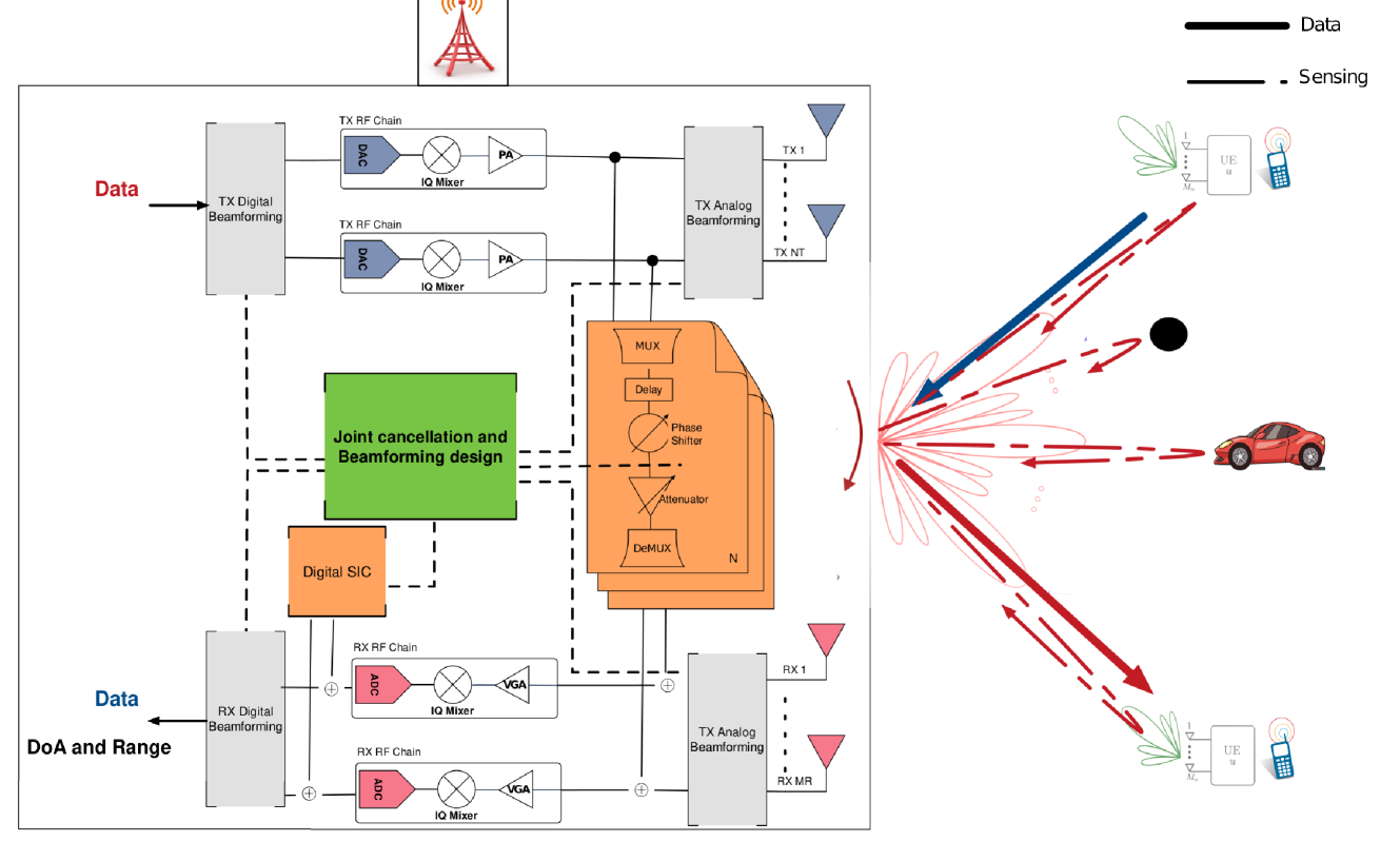
Figure 1: System Model for FD-ISAC – This example set $K$=4, 1 UL user, 1 DL user and 2 passive targets.

In the system model in the Fig. 1, we consider FD-ISAC communication system with a single BS comprising of partially connected HBF architecture at the TX and RX side and multiple targets, single DL and single UL user present in the vicinity of BS. Specifically, BS node $b$ consists of $N_{b}$ TX and $M_{b}$ RX antenna elements. The BS is communicating with DL user which consists of $M_{u}$ digital antenna elements and also with UL user which consists of $N_{u}$ digital antenna elements. The DL signal from the BS also reflects back from the multiple passive radar targets present in the environment. Regarding the HBF architecture at the BS there are a total of $N_{b}^{\text{RF}}$ RF chains at the TX and $M_{b}^{\text{RF}}$ RF chains at the RX. Each RF chain is connected to $N_{b}^{\text{A}}$ analog antennas at the TX and $M_{b}^{\text{A}}$ analog antennas at the RX.

For the communication and sensing, OFDM waveform is considered consisting of $P$ active subcarriers in each symbol and a total of $Q$ symbols. The frequency domain DL and UL symbol vectors at $p$-th sub-carrier and $q$-th symbol are represented as $\mathbf{s}_{b}^{p,q}$ and $\mathbf{s}_{u}^{p,q}$ respectively. At the BS, baseband (BB) data vector is precoded using digital beamformer matrix $\mathbf{V}_{b}^{\text{BB}}\in\mathbb{C}^{N_{b}^{RF}\times st}$ where $st$ represents data streams i.e., $st=\min\{N_{b}^{RF},M_{u}\}$. Following that, it is processed by analog beamformer $\mathbf{V}_{b}^{\text{RF}}\in\mathbb{C}^{N_{b}\times N_{b}^{RF}}$ containing a set of phase shifters as follows:

$${\mathbf{V}}_{b}^{{\text{RF}}}=\left[{\begin{array}[]{cccc}{{{\mathbf{v}}_{1}}}&{{{\mathbf{0}}_{N_{b}^{\text{A}}\times 1}}}&\cdots&{{{\mathbf{0}}_{N_{b}^{\text{A}}\times 1}}}\\ {{\mathbf{0}_{N_{b}^{\text{A}}\times 1}}}&{{{\mathbf{v}}_{2}}}&\cdots&{{{\mathbf{0}}_{N_{b}^{\text{A}}\times 1}}}\\ \vdots&\vdots&\ddots&\vdots\\ {{{\mathbf{0}}_{N_{b}^{\text{A}}\times 1}}}&{{{\mathbf{0}}_{N_{b}^{\text{A}}\times 1}}}&\cdots&{{{\mathbf{v}}_{N_{b}^{({\text{RF}})}}}}\end{array}}\right].$$ (1)

The elements of each $\mathbf{v}_{i}$ are assumed to have a constant modulus, i.e., $|[\mathbf{v}_{i}]_{n}|^{2}=1/N_{b}^{\text{A}}\,\,\forall n=1,2,\cdots,N_{b}^{\text{A}}$. It is also assumed that each vector in the analog beamformer belongs to some codebook, i.e., $\mathbf{v}_{i}\in\mathbb{F}_{\text{TX}}\forall i=1,2,\cdots,N_{b}^{\text{RF}}$. The RF domain DL signal at the BS can be written as $\mathbf{x}_{b}^{p,q}=\mathbf{V}_{b}^{\text{RF}}\mathbf{V}_{b}^{\text{BB}}\mathbf{s}_{b}^{p,q},$ with power constraint:

$$\mathbb{E}\left\{||\mathbf{V}_{b}^{\text{RF}}\mathbf{V}_{b}^{\text{BB}}\mathbf{s}_{b}^{p,q}||^{2}\right\}\leq\text{P}_{b}.$$

Similarly at the UL user, after digital precoding, the transmitted vector can be represented as $\mathbf{x}_{u}^{p,q}=\mathbf{V}_{u}^{\text{BB}}\mathbf{s}_{u}^{p,q}$, with power constraint:

$$\mathbb{E}\left\{||\mathbf{V}_{u}^{\text{BB}}\mathbf{s}_{u}^{p,q}||^{2}\right\}\leq\text{P}_{u}.$$

II-A Channel Models

For DL communication, it is assumed that there are $L$ scatterers present in the environment, which help to realize different line of sight (LOS) multipaths in DL channel. As mmWave system is assumed, Non line of sight (NLOS) paths are neglected. Hence, the DL channel can be given as

$$\mathbf{H}_{\text{DL}}=\sum_{l=1}^{L}\alpha_{l}\mathbf{a}_{M_{u}}(\theta_{l})\mathbf{a}_{N_{b}}^{\text{H}}(\theta_{l}),$$ (2)

where $\alpha_{l}\in\mathbb{C}$ and $\theta_{l}\in[-90\degree,90\degree]$ is the channel coefficient and angular direction of $l$-th path respectively. Moreover, $\mathbf{a}(\theta)$ is the uniform linear array (ULA) response vector and is given by:

$$\mathbf{a}_{N_{b}}(\theta)=\left[1,e^{j\frac{2\pi}{\lambda}d\sin(\theta)},\cdots,e^{j\frac{2\pi}{\lambda}(N_{b}-1)d\sin(\theta)}\right]^{\text{T}},$$

where $\lambda$ is the signal wavelength and $d$ is the inter-element spacing of the antenna array. For UL communication, only one direct LOS path is assumed. i.e.,

$$\mathbf{H}_{\text{UL}}=\beta\mathbf{a}_{M_{b}}(\phi)\mathbf{a}_{N_{u}}^{\text{H}}(\phi),$$ (3)

where $\beta$ is the UL channel coefficient and $\phi$ is the angular direction of user.

For sensing operation, it is assumed that there are $M$ passive radar targets, $L$ DL scatterers, and a single LOS reflection from UL user is considered. Hence total $K$ sensing targets are assumed i.e., $K=M+L+1$. The purpose of the sensing operation is to estimate the angular direction (Direction of Arrival (DoA)), range, and velocity of each radar target. The range and velocity of each target $k$ correspond to time delay $\tau_{k}$ and Doppler frequency $f_{D,k}$ respectively, such that $\tau_{k}=\frac{2d_{k}}{c}$ and $f_{D,k}=2v_{k}f_{c}/c$, where $c$ is the speed of light, $v_{k}$ is the velocity of $k$-th target and $f_{C}$ is the carrier frequency. Hence the radar channel at $p$-th subcarrier and $q$-th OFDM symbol can be given as

$$\mathbf{H}_{\text{Rad}}^{p,q}=\sum_{k=1}^{K}\alpha_{k}e^{j2\pi\left(qT_{s}f_{D,k}-p\tau_{k}\Delta f\right)}\mathbf{a}_{M_{b}}(\theta_{k})\mathbf{a}_{N_{b}}^{\text{H}}(\theta_{k}),$$ (4)

where $\alpha_{k}$ is the reflection coefficient of the $k$-th radar target, $\Delta f$ is the subcarrier spacing and $T_{s}=\frac{1}{\Delta f}+T_{cp}$ is the total symbol duration (including the cyclic prefix) and $\theta_{k}$ is the angular direction of the $k$-th target. The two-way propagation delay due to the range of the target translates to a phase shift across each subcarrier and the Doppler shift due to the moving velocity translates to a phase shift across each OFDM symbol. Moreover, in order to be consistent with UL channel, it is assumed that $\theta_{K}=\phi$.

II-B Received Signal Models

The DL signal received by the user at the $p$-th subcarrier and $q$-th OFDM symbol can be written as

$$\mathbf{y}_{u}^{p,q}=\mathbf{W}_{u}^{\text{H}}\left(\mathbf{H}_{\text{DL}}\mathbf{x}_{b}^{p,q}+\mathbf{z}_{u}^{p,q}\right),$$ (5)

where $\mathbf{W}_{u}$ is the digital RX beamformer and $\mathbf{z}_{u}^{p,q}\sim\mathcal{CN}(\mathbb{0},\sigma_{u}^{2}\mathbf{I}_{M_{u}})$ is the AWGN noise at the user. Similarly, the received signal at the RX of BS can be written as

$$\mathbf{y}_{b}^{p,q}=\underbrace{\mathbf{H}_{\text{Rad}}^{p,q}\mathbf{x}_{b}^{p,q}}_{\text{Radar Signal}}+\underbrace{\mathbf{H}_{b,b}\mathbf{x}_{b}^{p,q}}_{\text{\lx@glossaries@gls@link{acronym}{SI}{\leavevmode SI} signal}}+\underbrace{\mathbf{H}_{\text{UL}}\mathbf{x}_{u}^{p,q}}_{\text{\lx@glossaries@gls@link{acronym}{UL}{\leavevmode UL} signal}}+\mathbf{z}_{b}^{p,q},$$ (6)

where $\mathbf{z}_{b}^{p,q}\sim\mathcal{CN}(\mathbb{0},\sigma_{b}^{2}\mathbf{I}_{M_{b}})$ is the additive noise at the BS and $\mathbf{H}_{b,b}\in\mathbb{C}^{M_{b}\times N_{b}}$ is the SI channel path between BS TX and RX. The received signal is then processed with RF combiner matrix at the RX, which is designed similarly as 1. After RF combiner and A/D SI cancellation, the received signal is expressed as

$$\widetilde{\mathbf{y}}_{b}^{p,q}=\left(\mathbf{W}_{b}^{RF}\right)^{\text{H}}\left(\mathbf{H}_{\text{Rad}}^{p,q}\mathbf{x}_{b}^{p,q}+\mathbf{H}_{\text{UL}}\mathbf{x}_{u}^{p,q}\right)+\\ \left(\widetilde{\mathbf{H}}_{b,b}+\mathbf{C}_{b}+\mathbf{D}_{b}\right)\mathbf{V}_{b}^{\text{BB}}\mathbf{s}_{b}^{p,q}+\left(\mathbf{W}_{b}^{\text{RF}}\right)^{\text{H}}\mathbf{z}_{b}^{p,q},$$ (7)

where $\widetilde{\mathbf{H}}_{b,b}=\left(\mathbf{W}_{b}^{\text{RF}}\right)^{\text{H}}\mathbf{H}_{b,b}\mathbf{V}_{b}^{\text{RF}}$ and $\mathbf{C}_{b}$ and $\mathbf{D}_{b}$ are analog and digital cancellers and are designed by following the procedure presented in [6]. The expressions of $\mathbf{C}_{b}$ and $\mathbf{D}_{b}$ are derived based on the SI channel estimation $\widehat{\widetilde{\mathbf{H}}}_{b,b}$ as $\mathbf{C}_{b}=\Bigl{[}-\bigl{[}\widehat{\widetilde{\mathbf{H}}}_{b,b}\bigr{]}_{(:,1:\frac{N}{M_{b}^{\text{RF}}})}\,\boldsymbol{0}_{(:,N_{b}^{RF}-\frac{N}{M_{b}^{\text{RF}}}:N_{b}^{\text{RF}})}\Bigr{]}$ and $\mathbf{D}_{b}=-\bigl{(}\widehat{\widetilde{\mathbf{H}}}_{b,b}+\mathbf{C}_{b}\bigr{)}$, where $N$ is the number of analog canceller taps.
In order to extract the UL signal at the BS node $b$, a digital precoder is also applied at the RX of the node $b$. Hence the received signal after the digital combiner can also be written as

$$\widetilde{\mathbf{s}}_{b}^{p,q}=\left(\mathbf{W}_{b}^{\text{BB}}\right)^{\text{H}}\left(\mathbf{W}_{b}^{RF}\right)^{\text{H}}\bigl{(}\mathbf{H}_{\text{Rad}}^{p,q}\mathbf{x}_{b}^{p,q}+\mathbf{H}_{\text{UL}}\mathbf{x}_{u}^{p,q}\bigr{)}+\left(\mathbf{W}_{b}^{\text{BB}}\right)^{\text{H}}\\ \left(\widetilde{\mathbf{H}}_{b,b}+\mathbf{C}_{b}+\mathbf{D}_{b}\right)\mathbf{V}_{b}^{\text{BB}}\mathbf{s}_{b}^{p,q}+\left(\mathbf{W}_{b}^{\text{BB}}\right)^{\text{H}}\left(\mathbf{W}_{b}^{\text{RF}}\right)^{\text{H}}\mathbf{z}_{b}^{p,q}.$$ (8)

III Sensing Parameter Estimation

In this section, we present the parameter estimation of the sensing targets utilizing the received signal at the BS node $b$. We estimate the DoA, range, and velocity of the targets using both reflected and uplink signals at the BS RX.

First, we estimate the DoAs of targets including the direction of the DL and UL user using MUltiple SIgnal Classification (MUSIC) [18] parameter estimation algorithm. After receiving the $PQ$ snapshots of the reflected signal, we calculate the sample covariance matrix of (7). As the covariance matrix is positive semi-definite, after eigenvalue decomposition, all the eigenvalues will be real and non-negative. Now assuming $K<M_{b}^{\text{RF}}$, the subspace corresponding to the first $K$ eigenvalues will be signal space while the remaining subspace will correspond to noise subspace. In order to find the DoAs, $\widehat{\theta_{k}},\forall k$, we calculate the vectors orthogonal to noise subspace by sweeping through all the angles in angular range.

Second, we estimate the range and velocity of the radar targets, including DL and UL users, by finding out the delay and Doppler shift associated with the $K$ estimated DoAs. We formulate a reference signal in the $k$th target direction as

$$\begin{split}\mathbf{g}_{b,k}^{p,q}=\mathbf{a}_{M_{b}}(\widehat{\theta}_{k})\mathbf{a}_{N_{b}}^{\rm H}(\widehat{\theta}_{k})\mathbf{x}_{b}^{p,q}.\end{split}$$ (9)

The reference signal $\mathbf{g}_{b,k}^{p,q}$ in the direction of $\widehat{\theta}_{k}$ and the RX signal $\widetilde{\mathbf{y}}_{p,q}$ in (7) are utilized to derive quotient that includes the effect of delay and Doppler shift as

$$\begin{split}z_{b,k}^{p,q}=\frac{1}{M_{b}}\sum\limits_{i=1}^{M_{b}}[\mathbf{W}_{b}^{\rm RF}\widetilde{\mathbf{y}}_{b}^{p,q}]_{i}/[\mathbf{g}_{b}^{p,q}]_{i},\,\,\forall p,q.\end{split}$$ (10)

Now, we estimate the quantized delay and Doppler shift associated with $k$th radar target as

$$\begin{split}({n}^{*},{m}^{*})\!=\!\underset{n,m}{\text{arg max}}\Big{|}\!\sum\limits_{p=0}^{P-1}\!\Big{(}\!\!\sum\limits_{q=0}^{Q-1}z_{b}^{p,q}e^{-j2\pi\frac{qm}{Q}}\Big{)}e^{j2\pi\frac{pn}{P}}\Big{|}^{2}\end{split}$$ (11)

where $n=0,\cdots,P-1$ and $m=-Q/2,\cdots,Q/2-1$. Finally, the estimated delay and Doppler frequency are expressed as $\widehat{\tau}_{k}=\frac{{n}^{*}}{P\Delta f}$ and $\widehat{f}_{D,k}=\frac{{m}^{*}}{QT_{s}}$, respectively.

IV Proposed ISAC Optimization Framework

In this section, we propose an optimization framework for designing A/D beamformers such that the DL rate, sensing performance and UL rate get maximized while constraining SI power within a certain threshold.

We consider a time division duplexing communication protocol, where the DoAs estimated in one communication slot is utilized to derive the beamformers and SI cancellation matrices in the successive slot. The performance metrics for DL communication, UL communication and sensing are corresponding SINRs. The SINR for sensing echo can be given as

$$\gamma_{\text{rad}}=\frac{||\left(\mathbf{W}_{b}^{\text{RF}}\right)^{H}\widehat{\mathbf{H}}_{\text{Rad}}\mathbf{V}_{b}^{\text{RF}}\mathbf{V}_{b}^{\text{BB}}||_{\text{F}}^{2}}{||\left(\widehat{\widetilde{\mathbf{H}}}_{b,b}+\mathbf{C}_{b}+\mathbf{D}_{b}\right)\mathbf{V}_{b}^{\text{BB}}||_{\text{F}}^{2}+||\mathbf{W}_{b}^{\text{RF}}||^{2}\sigma_{b}^{2}},$$ (12)

where $\widehat{\mathbf{H}}_{\text{Rad}}=\sum_{i-1}^{K-1}\mathbf{a}_{M_{b}}(\widehat{\theta}_{i})\mathbf{a}_{N_{b}}^{\text{H}}(\widehat{\theta}_{i})+\mathbf{a}_{M_{b}}(\widehat{\phi})\mathbf{a}_{N_{b}}^{\text{H}}(\widehat{\phi})$, $\widehat{\widetilde{\mathbf{H}}}_{b,b}=(\mathbf{W}_{b}^{\text{RF}})^{\text{H}}\mathbf{H}_{b,b}\mathbf{V}_{b}^{\text{RF}}$ and $\mathbf{C}_{b}$. It is to be noted that the UL signal is not acting as the interference for the radar SINR, because we consider UL user as the active target present in the environment. Similarly the DL SNR is given by:

$$\gamma_{\text{DL}}=\frac{||\mathbf{W}_{u}^{H}\widehat{\mathbf{H}}_{\text{DL}}\mathbf{V}_{b}^{\text{RF}}\mathbf{V}_{b}^{\text{BB}}||_{\text{F}}^{2}}{||\mathbf{W}_{u}||^{2}\sigma_{u}^{2}},$$ (13)

where $\widehat{\mathbf{H}}_{\text{DL}}=\sum_{i=1}^{L}\mathbf{a}_{M_{u}}(\widehat{\theta}_{i})\mathbf{a}_{N_{b}}^{\text{H}}(\widehat{\theta}_{i})$. Moreover, for UL SINR, a digital combiner is used after RF combiner in order to extract the transmitted signal by the UL user. Hence the UL SINR is given by:

$$\gamma_{\text{UL}}=\frac{||\left(\mathbf{W}_{b}^{\text{BB}}\right)^{\text{H}}\left(\mathbf{W}_{b}^{\text{RF}}\right)^{\text{H}}\widehat{\mathbf{H}}_{\text{UL}}\mathbf{V}_{u}^{\text{BB}}||_{\text{2}}^{2}}{\Sigma_{\text{UL}}}$$ (14)

where $\Sigma_{\text{UL}}=||\left(\mathbf{W}_{b}^{\text{BB}}\right)^{\text{H}}\left(\mathbf{W}_{b}^{\text{RF}}\right)^{\text{H}}\widehat{\mathbf{H}}_{\text{Rad}}\mathbf{V}_{b}^{\text{RF}}\mathbf{V}_{b}^{\text{BB}}||_{\text{F}}^{2}+||\left(\mathbf{W}_{b}^{\text{BB}}\right)^{\text{H}}\left(\widehat{\widetilde{\mathbf{H}}}_{b,b}+\mathbf{C}_{b}+\mathbf{D}_{b}\right)\mathbf{V}_{b}^{\text{BB}}||_{\text{F}}^{2}+\sigma_{b}^{2}$ and $\widehat{\mathbf{H}}_{\text{UL}}=\mathbf{a}_{M_{b}}(\phi)\mathbf{a}_{N_{u}}^{\text{H}}(\phi)$.

The optimization problem to maximize the sensing SINR, DL SNR and UL SINR acn be written as

$$\begin{array}[]{c}\mathcal{O}\mathcal{P}:\mathop{\max}\limits_{\begin{array}[]{l}{\mathbf{V}}_{b}^{{\text{RF}}},{\mathbf{V}}_{b}^{{\text{BB}}},{\mathbf{W}}_{b}^{{\text{RF}}},\mathbf{W}_{b}^{\text{BB}},\\ {{\mathbf{C}}_{b}},{{\mathbf{D}}_{b}},\mathbf{V}_{u}^{\text{BB}},{{\mathbf{W}}_{u}}\end{array}}{{\gamma}_{{\text{Rad}}}}+{{\gamma}_{{\text{DL}}}}+\gamma_{\text{UL}}\\ {\text{s}}{\text{.t}}.{\left\|{{{\left[{\left({{{{\mathbf{\widehat{\widetilde{H}}}}}_{b,b}}+{{\mathbf{C}}_{b}}}\right){\mathbf{V}}_{b}^{{\text{BB}}}}\right]}_{(j,:)}}}\right\|^{2}}\leq{\lambda_{b}},\,\,\forall j=1,\ldots,M_{b}^{{\text{RF}}},\\ {\mathbb{E}}\left\{{{{\left\|{{\mathbf{V}}_{b}^{{\text{RF}}}{\mathbf{V}}_{b}^{{\text{BB}}}}\right\|}^{2}}}\right\}\leq{{\text{P}}_{b}}\\ \mathbb{E}\{||\mathbf{V}_{u}^{\text{BB}}||_{2}^{2}\}\leq\text{P}_{u}\\ {{\mathbf{w}}_{j}}\in{\mathbb{F}_{{\text{RX}}}}\forall j{\text{ and }}{{\mathbf{v}}_{n}}\in{\mathbb{F}_{{\text{TX}}}}\,\,\forall n=1,2,\ldots,N_{b}^{({\text{RF}})}\end{array}$$ (15)

Due to the coupling of optimization variables, the problem is non-convex and is challenging to solve. In this paper, an alternating optimization based solution is proposed.

The analog TX beamformer of BS is optimized such that the radar channel gain (numerator of (12)) gets maximized, which corresponds to a linear search through the codebook $\mathbb{F}_{\text{TX}}$. Similarly the optimization of BS RX beamformer is done such that radar channel return gets maximized and the SI power leakage gets minimized. This is again a linear search through the codebook $\mathbb{F}_{\text{RX}}$. This is further elaborated in Algorithm 1.

IV-A TX Digital Precoding

For designing digital TX precoder, the goal is to maximize the DL rate while minimizing SI power at the RX of node $b$. Hence following optimization problem is formalized: —s—[2] V_b^BB —— ^H_DL^effV_b^BB - G——_F^2 ——(V_b^BB)^Ht_r——_2^2   ≤   λ_b       ∀    r = 1, ⋯, M_b^RF ——[V_b^RFV_b^BB]_(:,c)——^2  ≤   P_b     ∀    c = 1, ⋯, st where $\widehat{\mathbf{H}}_{\text{DL}}^{\text{eff}}=\widehat{\mathbf{H}}_{\text{DL}}\mathbf{V}_{b}^{\text{RF}}$, $\mathbf{G}=\widehat{\mathbf{H}}_{\text{DL}}^{\text{eff}}\mathbf{V}\sqrt{\text{P}_{b}}$, where $\mathbf{V}$ is the right singular vectors of $\widehat{\mathbf{H}}_{\text{DL}}$ corresponding to largest singular values and $\mathbf{t}_{r}$ is the $r$-th row of the matrix $\widehat{\widetilde{\mathbf{H}}}_{b,b}+\mathbf{C}_{b}$ i.e., $\mathbf{t}_{r}=\left[\widehat{\widetilde{\mathbf{H}}}_{b,b}+\mathbf{C}_{b}\right]_{(r,:)}$. This is a convex optimization problem and for $M_{b}^{\text{RF}}=1$ solution is proposed using the Lagrangian method. The Lagrangian for this problem (ignoring constraint IV-A) can be written as

$$\mathcal{L}(\mathbf{V}_{b}^{\text{BB}},\zeta)=||\widehat{\mathbf{H}}_{\text{DL}}^{\text{eff}}\mathbf{V}_{b}^{\text{BB}}-\mathbf{G}||_{\text{F}}^{2}+\zeta(||(\mathbf{V}_{b}^{\text{BB}})^{\text{H}}\mathbf{t}_{1}||_{2}^{2}-\lambda_{b})$$ (16)

where $\zeta$ is the Lagrange multiplier. By taking the derivative with respect to each element of $\mathbf{V}_{b}^{\text{BB}}$ yields:

$$\frac{\partial}{\partial\mathbf{V}_{b}^{\text{BB}}}\mathcal{L}(\mathbf{V}_{b}^{\text{BB}},\zeta)=\left(\widehat{\mathbf{H}}_{\text{DL}}^{\text{eff}}\right)^{\text{H}}\widehat{\mathbf{H}}_{\text{DL}}^{\text{eff}}\mathbf{V}_{b}^{\text{BB}}-\left(\widehat{\mathbf{H}}_{\text{DL}}^{\text{eff}}\right)^{\text{H}}\mathbf{G}+\zeta\mathbf{t}_{1}\mathbf{t}_{1}^{\text{H}}\mathbf{V}_{b}^{\text{BB}}$$

The derivative of (16) with respect to lagrange multiplier $\zeta$ can be given as

$$\frac{\partial}{\partial\zeta}\mathcal{L}(\mathbf{V}_{b}^{\text{BB}},\zeta)=\mathbf{t}_{1}^{\text{H}}\mathbf{V}_{b}^{\text{BB}}(\mathbf{V}_{b}^{\text{BB}})^{\text{H}}\mathbf{t}_{1}-\lambda_{b}.$$

Equating both of these partial derivatives to zero will yield the optimal precoder and Lagrange multiplier $\accentset{\ast}{\zeta}$ i.e.,

$$\accentset{\ast}{\mathbf{V}}_{b}^{\text{BB}}=\left[\left(\widehat{\mathbf{H}}_{\text{DL}}^{\text{eff}}\right)^{\text{H}}\widehat{\mathbf{H}}_{\text{DL}}^{\text{eff}}+\accentset{\ast}{\zeta}\mathbf{t}_{1}\mathbf{t}_{1}^{\text{H}}\right]^{-1}\left(\widehat{\mathbf{H}}_{\text{DL}}^{\text{eff}}\right)^{\text{H}}\mathbf{G}$$ (17)

$$\mathbf{t}_{1}^{\text{H}}\mathbf{V}_{b}^{\text{BB}}(\mathbf{V}_{b}^{\text{BB}})^{\text{H}}\mathbf{t}_{1}=\lambda_{b}$$

Solving for $\zeta$ yields:

$$\accentset{\ast}{\zeta}=\frac{1}{{\mathbf{t}_{1}^{H}\left((\widehat{\mathbf{H}}_{\text{DL}}^{\text{eff}})^{\text{H}}\widehat{\mathbf{H}}_{\text{DL}}^{\text{eff}}\right)^{-1}\mathbf{t}_{1}}}\max\left(\frac{||\mathbf{t}_{1}||}{\sqrt{\lambda_{b}}}-1,0\right)$$ (18)

Inserting the $\accentset{\ast}{\zeta}$ value in (17) will yield optimal digital precoder. Here we assume that the inverse of $\left((\widehat{\mathbf{H}}_{\text{DL}}^{\text{eff}})^{\text{H}}\widehat{\mathbf{H}}_{\text{DL}}^{\text{eff}}\right)$ exists. While solving the problem IV-A, the constraint (IV-A) is not considered. This constraint is forced by normalizing each vector of the precoder matrix by $\text{P}_{b}$ if it does not satisfy the constraint (IV-A) i.e.,

$$\left[\mathbf{V}_{b}^{\text{RF}}\accentset{\ast}{\mathbf{V}}_{b}^{\text{BB}}\right]_{(:,c)}=\frac{\left[\mathbf{V}_{b}^{\text{RF}}\accentset{\ast}{\mathbf{V}}_{b}^{\text{BB}}\right]_{(:,c)}}{\Bigl{|}\Bigl{|}\left[\mathbf{V}_{b}^{\text{RF}}\accentset{\ast}{\mathbf{V}}_{b}^{\text{BB}}\right]_{(:,c)}\Bigr{|}\Bigr{|}}\sqrt{\text{P}_{b}}\,\,\,\forall c=1,\cdots,st$$ (19)

IV-B RX Digital combiner

After radar processing of the received signal, a digital combiner is applied for the extraction of UL signal. As mentioned in (14), the radar signal acts as an interference to the UL signal. Hence in order to maximize UL SINR (14), NSP method is proposed to minimize the radar interference. In order to do that virtual radar channel is formulated without considering the UL user as a target i.e.,

$$\widehat{\mathbf{H}}_{\text{Rad,Int}}=\sum_{i=1}^{K-1}\mathbf{a}_{M_{b}}(\widehat{\theta}_{i})\mathbf{a}_{N_{b}}^{\text{H}}(\widehat{\theta}_{i})$$ (20)

The optimization problem for designing digital RX precoder then can be formulated as —s—[2] W_b^BB —— (W_b^BB)^H⏟(W_b^RF)^H^H_UL_^H_UL^eff——_F^2 (W_b^BB)^H⏟(W_b^RF)^H^H_Rad,Int_^H_Rad,Int^eff = 0

In order to maximize the (IV-B), the $\mathbf{W}_{b}^{\text{BB}}$ can be chosen as the left singular vectors of matrix $\mathbf{H}_{\text{UL}}^{\text{eff}}$ corresponding to largest singular values. Hence the objective function (IV-B) can be reformulated into the least squares function i.e., $\underset{\mathbf{W}_{b}^{\text{BB}}}{\min}\,||\mathbf{W}_{b}^{\text{BB}}-\mathbf{X}||_{\text{F}}^{2}$, with the same constraint (IV-B), where $\mathbf{X}$ is the left singular vectors of matrix $\widehat{\mathbf{H}}_{\text{UL}}^{\text{eff}}$ corresponding to largest singular values. This reformulated problem is a well-studied problem and the solution is given as the NSP of the matrix $\left(\widehat{\mathbf{H}}_{\text{Rad,Int}}^{\text{eff}}\right)^{\text{H}}$ [19]. The optimal digital combiner can be given as

$$\accentset{\ast}{\mathbf{W}}_{b}^{\text{BB}}=\left(\mathbf{I}-\mathbf{A}^{\text{H}}\left(\mathbf{A}\mathbf{A}^{\text{H}}\right)^{-1}\mathbf{A}\right)\mathbf{X},$$ (21)

where $\mathbf{A}=\left(\widehat{\mathbf{H}}_{\text{Rad,Int}}^{\text{eff}}\right)^{\text{H}}$.

Each vector in the designed matrix will further be normalized to the unit norm. Our procedure for solving the optimization problem 15 has been summarized in Algorithm 1.

Algorithm 1 FD-ISAC Optimization

Input: $\widehat{\mathbf{H}}_{b,b},\widehat{\mathbf{H}}_{\text{DL}},\widehat{\mathbf{H}}_{\text{UL}},\widehat{\mathbf{H}}_{\text{Rad}},\text{P}_{b},\text{P}_{u}$ and $\widehat{\theta}_{k}$ (Using MUSIC [18]) $\forall k$
Output: $\mathbf{V}_{b}^{\text{RF}},\,\mathbf{V}_{b}^{\text{BB}},\,\mathbf{W}_{b}^{\text{RF}},\,\mathbf{W}_{b}^{\text{BB}},\,\mathbf{W}_{u},\,\mathbf{V}_{u}^{\text{BB}},\,\mathbf{C}_{b},\,\mathbf{D}_{b}$

1:Set $\mathbf{W}_{u}^{\text{BB}}$ as the $st$ left singular vectors of $\widehat{\mathbf{H}}_{\text{DL}}$ corresponding to largest singular values.

2:Set ${\mathbf{V}}_{b}^{{\text{RF}}}=\mathop{\operatorname{argmax}}\limits_{{{\mathbf{v}}_{j}}\in{\mathbb{F}_{{\text{TX}}}}}{\left\|{{{{\mathbf{\widehat{H}}}}_{\text{Rad}}}{\mathbf{V}}_{b}^{{\text{RF}}}}\right\|^{2}}$.

3:Set ${\mathbf{W}}_{b}^{{\text{RF}}}=\mathop{\operatorname{argmax}}\limits_{{{\mathbf{w}}_{j}}\in{\mathbb{F}_{{\text{TX}}}}}\frac{{{{\left\|{{{\left({{\mathbf{W}}_{b}^{{\text{RF}}}}\right)}^{\text{H}}}{{{\mathbf{\widehat{H}}}}_{\text{R}}}{\mathbf{V}}_{b}^{{\text{RF}}}}\right\|}^{2}}}}{{{{\left\|{{{\left({{\mathbf{W}}_{b}^{{\text{RF}}}}\right)}^{\text{H}}}{{{\mathbf{\widehat{H}}}}_{{\text{b}},{\text{b}}}}{\mathbf{V}}_{b}^{{\text{RF}}}}\right\|}^{2}}}}$.

4:Construct $\widehat{\widetilde{\mathbf{H}}}_{b,b}=\left(\mathbf{W}_{b}^{\text{RF}}\right)^{\text{H}}\widehat{\mathbf{H}}_{b,b}\mathbf{V}_{b}^{\text{RF}}$ and $\widehat{\mathbf{H}}_{\text{DL}}^{\text{eff}}=\widehat{\mathbf{H}}_{\text{DL}}\mathbf{V}_{b}^{\text{RF}}$.

5:Set $\mathbf{C}_{b}$ and $\mathbf{D}_{b}$.

6:if $M_{b}^{RF}=1$ then

7:     Set $\accentset{\ast}{\zeta}$ as defined in (18).

8:     Set ${\mathbf{V}}_{b}^{\text{BB}}$ as defined in (17) after solving problem in IV-A.

9:else

10:     Use numerical optimization techniques to solve problem in IV-A.

11:end if

12:Set $\mathbf{V}_{u}^{\text{BB}}$ as the first right singular vector of $\widehat{\mathbf{H}}_{\text{UL}}$ corresponding to largest singular value.

13:Set $\mathbf{W}_{b}^{\text{BB}}$ as defined in (21) after solving problem IV-B.

V Numerical Results

In this section, we present numerical results for our proposed FD-ISAC system. The simulation parameters have been provided in the table I. In addition to that, a radio subframe of 1ms has been assumed for DL communication. The RXs have an effective dynamic range of 60 dB provided by 14-bit Analog-to-Digital Converter (ADC) for a Peak-to-Average-Power-Ratio (PAPR) of 10 dB. Therefore, the residual SI power after analog cancellation at each RF chain has to be below -30 dBm to avoid signal saturation. Moreover, the SI channel has been modeled as a Rician fading channel with a $\kappa$ value of 35 dB and path loss of 40 dB. For a BS analog TX/RX beamformer, we consider a 5-bit beam codebook based on discrete fourier transform (DFT) matrix.

TABLE I: Simulation Parameters

Simulation Parameters
Parameter Name	Symbol	Parameter value
Carrier Frequency	$f_{c}$	28 GHz
TX RF chains	$N_{b}^{\text{RF}}$	8
RX RF chains	$M_{b}^{\text{RF}}$	8
TX Antennas per RF chain	$N_{b}^{A}$	16
RX Antennas per RF chain	$M_{b}^{A}$	16
Active Subcarriers	P	792
OFDM Symbols	Q	14
Symbol Duration	$T_{s}$	8.92 $\micro s$
RX Noise Floor	$\sigma_{b}^{2},\sigma_{u}^{2}$	-90 dBm
RX RF saturation level	$\lambda_{b}$	-30 dBm

V-A Sensing Performance

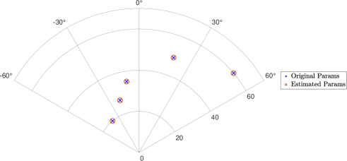
Figure 2: Range Angle Profile for TX power of 30 dBm. The DL link is associated with $L=2$ scatteres at $\theta_{1}=-30\degree$ and $\theta_{2}=-20\degree$. The UL user is present at the angle $\phi=-10\degree$.

In Fig. 2 the sensing performance of the proposed system is shown with a DL transmit power of $30$ dBm and UL transmit power of $10$ dBm. It can be seen that the estimated and original target parameters nearly overlap each other. Moreover, we also estimated the UL user parameters (at $\phi=-10\degree$) without treating the UL user as an interference to radar signal. Hence it showed that UL user signal does not interfere with radar estimation as far as UL user is treated as a potential target. The high angular resolution is due to MUSIC DoA estimation, which is known to give highly accurate results as far $K<M_{b}^{\text{RF}}$. If $K>M_{b}^{\text{RF}}$ then one can use the conventional beam scanning approach to estimate DoAs.

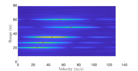
Figure 3: Range - Velocity Profile for TX Power $\text{P}_{b}=30$ dBm.

In Fig. 3 the range-velocity profile of the proposed system is shown. The map is obtained by implementing the range-velocity estimation algorithm individually for each target and then adding the maps after normalizing each one with the max value. It can be seen that the targets are easily recognizable across the range axis as compared to the velocity axis. This is because $Q<<P$. Hence the number of samples across which the velocity is being measured is much less than the samples for range estimation. Applying the range and velocity estimation over the larger subset of OFDM symbols will improve the velocity resolution.

V-B DL rate performance

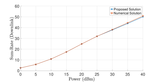
Figure 4: Effect pf proposed solution and numerical solution of TX precoder design on Sum-Rate (bps/Hz) with $N_{b}^{\text{RF}}=5,\,M_{b}^{\text{RF}}=1,\,M_{u}=5,\,L=5$. The rest of the system parameters are taken from table I. The horizontal axis is the transmit power of BS ($\text{P}_{b}$).

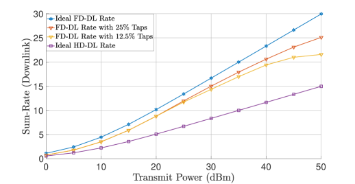
Figure 5: DL rate (bps/Hz) Performance using 128$\times$128 BS node and 4 antenna UE RX node

In Fig. 4, the verification of the proposed DL precoder is presented. DL rate is taken as the performance metric for the DL precoder design. It can be seen that the proposed solution is approximately matches with the numerical solution, which is computed through numerically solving the the convex optimization problem (IV-A) using CVX. Moreover, even when the SI leakage is high (at high transmit power), our proposed algorithm manages to provide a considerably better DL rate.

In Fig. 5, DL rate performance is presented. For ideal rate calculation, a system having no SI and radar channel is considered and all of beamformers are optimized in order to maximize the DL rate. It can be seen that despite having SI channel interference and radar targets in the environment, the proposed system is able to provide DL rate which is very close to the ideal rate. Moreover, if we increase the analog SI cancellation taps at the BS, DL rate and sensing performance improve as A/D beamformers are utilized to increase the rate and sensing performance. In the high transmit power regime, the SI interference also scales up, and hence the system will utilize more resources to lessen the SI signal and this will cause the DL rate and sensing performance to deteriorate.

V-C UL rate performance

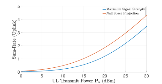
Figure 6: UL rate (bps/Hz) performance with 4 antenna UE TX node and the BS TX power $\text{P}_{b}=30\text{ dBm}$.

Fig. 6 depicts the UL rate performance of the proposed system against UL transmit power. The proposed NSP method of receiver digital precoder has been compared with maximum signal strength (MSS) method where $\mathbf{W}_{b}^{\text{BB}}$ has been chosen as the left singular vectors of $\mathbf{H}_{\text{UL}}^{\text{eff}}$ without considering the constraint (IV-B). It can be observed that the proposed method constantly provides a better UL sum-rate than the MSS. It is because, in MSS as we are not forcing our precoder to belong to the null space of $\mathbf{H}_{\text{rad,Int}}^{\text{eff}}$, the radar signal act as a strong interference to the UL signal which suppresses the UL SINR and ultimately the rate.

VI Conclusion

In this article, we presented FD-ISAC communication system with multiple targets and UL and DL communication users. We proposed a complete framework for maximizing the DL and UL rate performance while also estimating the targets’ radar parameters (DoA, range and velocity). We optimize the A/D beamformers at both TX and RX of BS and users to increase the corresponding SINRs and to minimize the SI leakage power at BS. Our results demonstrated accurate radar parameter estimation and increased DL and UL rates. Moreover, our proposed algorithm manages to provide a high DL rate even at high SI leakage.

References

• [1] “The next hyper-Connected experience for all.” White Paper, June 2020.
• [2] K. V. Mishra et al., “Toward millimeter-wave joint radar communications: A signal processing perspective,” IEEE Signal Process. Mag., vol. 36, pp. 100–114, Sep. 2019.
• [3] B. Smida, A. Sabharwal, G. Fodor, G. C. Alexandropoulos, H. A. Suraweera, and C. Chae, “Full-duplex wireless for 6G: Progress brings new opportunities and challenges,” IEEE J. Sel. Areas Commun., vol. 41, pp. 2729–2750, Sep. 2023.
• [4] S. P. Chepuri, N. Shlezinger, F. Liu, G. C. Alexandropoulos, S. Buzzi, and Y. C. Eldar, “Integrated sensing and communications with reconfigurable intelligent surfaces: From signal modeling to processing,” IEEE Signal Process. Mag., vol. 40, pp. 41–62, Sep. 2023.
• [5] G. C. Alexandropoulos, M. A. Islam, and B. Smida, “Full duplex massive MIMO architectures: Recent advances, applications, and future directions,” IEEE Veh. Technol. Mag., vol. 17, pp. 83–91, Dec. 2022.
• [6] G. C. Alexandropoulos and M. Duarte, “Joint design of multi-tap analog cancellation and digital beamforming for reduced complexity full duplex MIMO systems,” in Proc. IEEE ICC, (Paris, France), May 2017.
• [7] M. A. Islam, G. C. Alexandropoulos, and B. Smida, “Simultaneous downlink data transmission and uplink channel estimation with reduced complexity full duplex MIMO radios,” in Proc. IEEE Intl. Conf. Commun. (ICC), pp. 1–6, Jun. 2020.
• [8] C. B. Barneto et al., “Beamforming and waveform optimization for OFDM-based joint communications and sensing at mm-waves,” in Proc. IEEE ASILOMAR, (Pacific Grove, USA), pp. 895–899, Nov. 2020.
• [9] S. D. Liyanaarachchi et al., “Joint multi-user communication and MIMO radar through full-duplex hybrid beamforming,” in IEEE Int. Symp. Joint Commun. & Sensing, pp. 1–5, Feb. 2021.
• [10] M. A. Islam, G. C. Alexandropoulos, and B. Smida, “Simultaneous multi-user MIMO communications and multi-target tracking with full duplex radios,” in Proc. IEEE Global Commun. Conf. (GLOBECOM), pp. 1–6, Dec. 2022.
• [11] M. A. Islam, G. C. Alexandropoulos, and B. Smida, “Integrated sensing and communication with millimeter wave full duplex hybrid beamforming,” in Proc. IEEE Intl. Conf. Commun. (ICC), pp. 1–6, May 2022.
• [12] C. B. Barneto, T. Riihonen, S. D. Liyanaarachchi, M. Heino, N. González-Prelcic, and M. Valkama, “Beamformer design and optimization for joint communication and full-duplex sensing at mm-waves,” IEEE Transactions on Communications, vol. 70, no. 12, pp. 8298–8312, 2022.
• [13] J. Pritzker, J. Ward, and Y. C. Eldar, “Transmit precoding for dual-function radar-communication systems,” in 2021 55th Asilomar Conference on Signals, Systems, and Computers, pp. 1065–1070, 2021.
• [14] I. Gavras, M. A. Islam, B. Smida, and G. C. Alexandropoulos, “Full duplex holographic MIMO for near-field integrated sensing and communications,” in Proc. European Signal Proces. Conf., (Helsinki, Finland), Sep. 2023.
• [15] T. Gong, P. Gavriilidis, R. Ji, C. Huang, G. C. Alexandropoulos, L. Wei, M. Debbah, H. V. Poor, and C. Yuen, “Holographic MIMO communications: Theoretical foundations, enabling technologies, and future directions,” IEEE Commun. Surveys Tuts., to appear, 2023.
• [16] C. K. Sheemar, G. C. Alexandropoulos, D. Slock, J. Querol, and S. Chatzinotas, “Full-duplex-enabled joint communications and sensing with reconfigurable intelligent surfaces,” in Proc. European Signal Proces. Conf., (Helsinki, Finland), Sep. 2023.
• [17] Z. Liu, S. Aditya, H. Li, and B. Clerckx, “Joint transmit and receive beamforming design in full-duplex integrated sensing and communications,” IEEE Journal on Selected Areas in Communications, vol. 41, no. 9, pp. 2907–2919, 2023.
• [18] R. Schmidt, “Multiple emitter location and signal parameter estimation,” IEEE Transactions on Antennas and Propagation, vol. 34, no. 3, pp. 276–280, 1986.
• [19] D. P. Bertsekas, “Nonlinear programming,” J. Operational Research Society, vol. 48, no. 3, pp. 334–334, 1997.