”SNe Ia twins for life” towards a precise determination of H₀

Abstract

Here we present an approach to the measurement of extragalactic distances using twin SNe Ia, taken from the early down to the nebular phase. The approach is purely empirical, although we can give a theoretical background on why the method is reliable. Studying those twins in galaxies where peculiar velocities are relatively unimportant, we can tackle the H₀ tension problem. Here we apply the method to the determination of the distances to NGC 7250 and NGC 2525, who hosted respectively SN 2013dy and SN 2018gv, twins of two different SNe Ia prototypes: SN 2013aa/ SN 2017cbv and SN2011fe. From the study of the SN 2013aa and SN 2017cbv twin pair, by comparing it with SN 2011fe and applying the difference between the SN 2013aa/2017cbv and the SN 2011fe class, we find as well a good estimate of the distance to NGC 5643. Our study points to distances consistent with the Cepheids distance estimates by SH0ES in NGC 7250 and NGC 2525 (within 1$\sigma$ errors). (Note that no TRGB distances are available for NGC 7250 and NGC 2525). We get, on the other hand, a good agreement with the distance estimates for M101 and NGC 5643 with the TRGB method. We just have started to measure distances with this method for the samples in Freedman et al (2019) and Riess et al (2022). Though there are differences in measured distances to the same galaxy using Cepheids or the TRGB, the Hubble tension can arise as well from the corrections of peculiar velocities of nearby galaxies which are not in the Hubble flow. Thus, we expect to apply the method in galaxies with z $>$0.02–0.03 well into the Hubble flow to obtain a reliable value for H₀ with the use of the ELT or the JWST.

1 Introduction

Type Ia supernovae (SNe Ia) at high $z$ led to the discovery of the acceleration of the Universe (Riess et al. 1998; Perlmutter et al. 1999) and of the presence of a repulsive dynamical component that permeates it and accounts for such accelerated expansion. This component is known as dark energy and its nature is the subject of present and future research.

Apart from such endeavour in the field of very large $z$ (see the latest developments in Rubin et al. 2023), there is, at low $z$ a very important question to solve: the Hubble tension. This is a well known tension between the value of the Hubble constant H₀ derived from the CMB by the Planck collaboration and that obtained, using Cepheids, by Riess and co-workers in their SH0ES program. The CMB value of H₀ = 67.4$\pm$0.5 km s^-1 Mpc^-1 (Planck Collaboration 2020) and the latest SH0ES value of H₀ = 73.29$\pm$0.9 km s^-1 Mpc^-1 (Murakami et al et. 2023) have now a discrepancy at the 5.7 $\sigma$ level.

Such difference in H₀ questions seriously the $\Lambda$CDM model and some authors claim the need of new physics in the early Universe to make the Planck value compatible with that derived by methods involving low-$z$ astrophysical distance indicators such as Cepheids (see Di Valentino et al. 2021 for a review). An exploration for a possible consistency of the CMB Planck data with the SH0ES H₀ has been done (see the early attempt by Bernal, Verde and Riess in 2016 for instance), but (see Efstathiou, Rosenberg and Poulin 2023, amongst others) no solution consistent with the $\Lambda$CDM model appears satisfactory.

The situation, however, is not completely clear, since there are methods that do not use Cepheids and predict values of H₀ in-between those from Planck and from SH0ES. So, using the Tip of the Red Giant Branch (TRGB) method, Freedman et al. (2019) found a value of H₀ = 69.8$\pm$0.8 (stat)$\pm$1.7 (sys) km s^-1 Mpc^-1. They noted a mean difference in galaxy moduli $\mu^{TRGB}-\mu^{Ceph}$ = 0.059 mag. The scatter is significantly larger for the distant galaxies than for the nearby ones, where it amounts to $\pm$ 0.05 mag only.

On the other hand, the sample of distances obtained by the Surface Brightness Fluctuations (SBF) method, dominated by early-type galaxies, which is required by the method, show a mean difference of $\mu^{SFB}-\mu^{Ceph}$ = 0.07 mag between the distances estimated using SFB and those using the Cepheid calibration (Khetan et al. 2021). A value of H₀ =70.50 $\pm$ 2.37 (stat) $\pm$ 3.38 (sys) km s^-1 Mpc^-1 is derived in that paper. This, however, has been questioned by Blakeslee et al. (2021), obtaning an H₀ around 73 km s^-1 Mpc^-1.

In general, there are promising ideas to give an estimate of H₀, but different applications of the methods lead also to different results (see the review by Freedman & Madore 2023, for instance).

To determine the value of H₀ from the distances to galaxies which are not yet in the Hubble flow, corrections for peculiar velocities must be applied. These corrections are made differently in the various approaches and may be, in part, responsible for the discrepant results.

It must be noted that the Tip of the Red Giant Branch and Cepheid distance scale relies on three rungs: (1) Local anchors (Milky Way, LMC, maser host NGC 4258), (2) Cepheid or Tip of the Red Giant Branch (TRGB) distances to Type Ia supernovae (SNIa) host galaxies and (3) SNIa distances in the Hubble flow. The step 2 and 3 can be responsible of the different result in H₀ as there are differences in the distances in step 2 gathered by these two methods, and there are differences in step 3 involved in the different treatment of peculiar velocities by the two methods.

We note that Kenworthy et al. (2022) studying the uncertanties in the peculiar velocities obtained by various models brings H₀ from the use of Cepheids in 35 extragalactic hosts to a range from 71.8 to 77 km s^-1 Mpc^-1. So the actual SH0ES value for H₀ becomes 73.1 ${}^{+2.6}_{-2.3}$ km s^-1 Mpc^-1, at 2.6 $\sigma$ tension with Planck.

Here we address the step 2 of the rungs in a couple of galaxies that hosted twin SNe Ia. We hope in the future to avoid the modelling of peculiar velocities and jump one rung in the distance ladder by going directly to host galaxies of SNe Ia at z $\sim$ 0.02-0.03.

The use of SNe Ia as distance indicators for cosmology was only made possible when the correlation between maximum brightness and rate of decline in the light curve was formulated in a general, quantitative way by Phillips (1993). Later on, further ways to formulate such correlation have been the stretch $s$, first introduced by Perlmutter et al. (1999), the Multi Light Curves Shape (MLCSk2) (Riess, Press & Kirshner 1995; Jha et 2007), or the stretch $x1$ (Guy et al. 2005), which go beyond the parameterization by $\Delta m_{15}$ (magnitude different between peak brightness and that 15 days later) of the decline rate introduced by Phillips (1993). One current advance in achieving a more precise use of the rate of decline of the SNe Ia to standardize them is the inclusion of twin embedding (Fakhouri et al. 2015; Boone et al. 2016). It started when Fakhouri et al. (2015) found that by using SN Ia pairs with closely matching spectra, from the SNFactory sample, they achieved a reduced dispersion in brightness. They were able to standardize high-redshift SNe to within 0.06–0.07 mag. The idea is most promising, given the expected massive gathering of SNe Ia spectra at high $z$. Twins are used there to connect the absolute magnitude estimate at maximum brightness with parameters corresponding to the spectral diversity of the SNe Ia. The method is well suited for the time when dark energy is entering in the Hubble diagram, allowing to determine $\Omega_{M}$ and $\Omega_{DE}$, as well as the equation of state of dark energy.

In the present paper we propose to use ”SNe Ia twins for life”, from early to the nebular phases. It is a use of SNe Ia to address the Hubble tension issue which uses the spectral evolution of those SNe Ia which have not only similar stretch but identical features along the lifetime of the SNe Ia. The precision of the distance provided by those twins should be larger than for SNe Ia with just similar stretch.

The method does not start from the apparent magnitudes of the SNe Ia, but from their spectra, with particular emphasis on those from the nebular phase, which are very sensitive to the reddening and to the intrinsic luminosity of the SNe. To get a direct check of the distance ladder, we make an empirical use of twin SNe Ia by comparing their spectra all the way from the early until the nebular phase. We obtain a good estimate of the relative distances between SNe Ia which are in different galaxies but seem identical spectroscopically, in addition to having a similar stretch. It is important, here, that the SNe Ia do show twin behaviour through the SN Ia life. Given the range of diversity of the SNe Ia already sampled, it should always be possible to find some of them with spectra similar to those of any newly discovered SN Ia. As nearby SNe Ia will be observed by the thousands per month with the advent of the LSST, it will be possibly to match their spectra with those of distant SNe Ia and then gain a new perspective on the extragalactic distance scale. Extending this procedure to reach SNe Ia that are in the Hubble flow should allow to avoid using a fiducial absolute magnitude M_B–H₀ relation, and get a direct comparison of distances leading straightforwardly to the value of H₀.

The gain of using the ”twins for life” approach is that it provides a direct measurement of distance, intrinsic color and reddening caused by Galactic and extragalactic dust by the use of the whole spectra of the SN Ia. It allows the consistent pairing of SNe Ia through all phases. The selection of twins is made of SNe Ia with a similar stretch, being then of similar luminosities, but in addition the ”twinness factor” can make more precise the distance estimate. So, all this makes a vey useful tool to gather the right distance ladder.

In section 2, we describe the method and characterize what is a perfect twin against other ways to compare SNe Ia. In section 3, we obtain the distance to NGC 7520, the host galaxy of SN 2013dy. In section 4, we obtain the distance to NGC NGC 2525, the host galaxy of SN 2018gv. In section 5 we compare our results within the SNe Ia diversity and discuss them. In section 6 we give our conclusions.

2 Purely empirical twins until the nebular phase

The key to this approach is to have a nearby SN Ia of the same type as another at much longer distance. For the nearby SN Ia, a good distance determination should be available. We will demonstrate this by using SN 2013dy in NGC 7520, which is a twin of SN2017cbv/SN2013aa both in NGC 5643.

Table 1 show the references for the spectra and photometry used in this paper. Some spectra have been provided generously by various researchers, and some others have been taken from the WISeREP. All are carefully calibrated in flux in agreement with the published photometry. The error in the flux calibration is well taken into account.

Table 1: Spectra and photometry of the SNe Ia twins sample

Spectra
SN	Galaxy	MJD	Phase (days)	Reference∗	Comments
2013aa	NGC 5643	56341	-2	Burns et al. (2020)	Priv. comm.
$\dots$	$\dots$	56391	+48	*
$\dots$	$\dots$	56676	+333	*
$\dots$	$\dots$	56704	+361	*
2017cbv	NGC 5643	57836	-2	Burns et al. (2020)	Priv. comm.
$\dots$	$\dots$	58171	+333	*
$\dots$	$\dots$	58199	+361	*
2013dy	NGC 7250	56498	-2	Pan et al. (2015)
$\dots$	$\dots$	56546	+46	Zhai et al. (2016)
$\dots$	$\dots$	56833	+333	Zhai et al. (2016)
2011fe	M101	55823	+9	Zhang et al. (2016)
$\dots$	$\dots$	56103	+289	Mazzali et al. (2015)
$\dots$	$\dots$	56158	+344	*
2018gv	NGC 2525	58159	+9	*
$\dots$	$\dots$	58439	+289	Graham et al. (2022)	Priv. comm.
$\dots$	$\dots$	58494	+344	Graham et al. (2022)	Priv. comm.
Photometry
2013aa	—	—	—	Burns et al. (2020)	—
2017cbv	—	—	—	Burns et al. (2020)	—
2013dy	—	—	—	Pan et al. (2015)	—
2011fe	—	—	—	Zhang et al. (2016)	—
2018gv	—	—	—	Scolnic et al. (2022)	—
* Spectrum from the WISeREP.

Table 2: SN 2013aa and SN 2017cbv

SN 2013aa
RA, DECa	14:32:33.881	-44:13:27.80
Discovery datea	$\dots$	2013-02-13
Phase ( referred to maximum light)b	$\dots$	-7 days
Redshiftc	$\dots$	0.004
E(B-V)MWd	$\dots$	0.15$\pm$0.06 mag
$m_{B}^{max}$ b	$\dots$	11.094$\pm$0.003 mag
$\Delta m(B)_{15}$b	$\dots$	0.95$\pm$0.01
Stretch factor $s_{BV}^{D}$b	$\dots$	1.11$\pm$0.02
Phases of the spectra used	$\dots$	-2, 360-370 days
SN 2017cbv
RA, DECe	14:32:34.420	-44:08:02.74
Discovery datee	$\dots$	2017-03-10
Phase (referred to maximum light)b	$\dots$	-18 days
Redshiftc	$\dots$	0.004
E(B-V)MWd	$\dots$	0.15$\pm$0.06 mag
$m_{B}^{max}$ b	$\dots$	11.11$\pm$0.03 mag
$\Delta m(B)_{15}$b	$\dots$	0.96$\pm$0.02
Stretch factor $s_{BV}^{D}$b	$\dots$	1.11$\pm$0.03
Phases of the spectra used	$\dots$	-2, 360-370 days

aWaagen (2013).	bBurns et al. (2020).	cParrent et al. (2013).
dSchlafly & Finkbeiner (2011).	eTartaglia et al. (2017).

We first check the method by taking two twin SNe Ia that are at the same distance and share the same reddening: SN 2017cbv/SN 2013aa.

2.1 Testing the method with twin SNe Ia in NGC 5643

SN 2013aa and SN 2017cbv appeared in the same galaxy, NGC 5643. They had similar decline rates and similar B-peak magnitudes. The studies done on these two SNe Ia also reveal similar characteristics in other aspects. Table 1 specifies the decline rates of those SNe Ia not only by $\Delta m_{15}(B)$ but also by s${}_{BV}^{D}$ (Burns et al. 2020).

Burns et al. (2014) showed that the color-stretch parameter is a robust way to classify SNe Ia in terms of light-curve shape and intrinsic colors. They propose a way to quantify the decline rate of the SNe directly from photometry, by just determining the epoch when the B–V color curves reach their maxima (i.e., when the SNe are reddest) relative to the that of the B-band maximum. Dividing this time interval by 30 days then gives the observed color-stretch parameter s${}_{BV}^{D}$. the “D” in the superindex refering to the direct comparison in B, without having to take into account the BVRI light curves.

The problems involved in the use of $\Delta m_{15}(B)$ are known. The first one is that the decline in 15 days past maximum can take (and it often does) differing values in different authors. Phillips et al. (1999), noted in addition that any reddening undergone by the SN would change the shape of the B-band light-curve and therefore the observed value of $\Delta m_{15}(B)$. A similar problem is that, by definition, $\Delta m_{15}(B)$ is tied to a particular photometric system, and so will vary from data set to data set and will require S-corrections (Suntzeff et al. 1988; Stritzinger et al. 2002) to convert one set of $\Delta m_{15}(B)$ to another. And lastly, $\Delta m_{15}(B)$ is defined by measuring the light curve at two very specific epochs, and some form of interpolation is usually needed to obtain these values.

Fitting the B-V color curves with cubic splines, Burns et al (2020) find identical color-stretch s${}_{BV}^{D}$ = 1.11 for SN 2013aa and SN 2017cbv. This value is smaller (slower decline) than in typical SNe Ia. They also found similar values in the Branch classification, concerning the equivalent widths (EW) of the lines of different elements. This proves that their interior was very alike in chemical composition.

SN 2013aa and SN 2017cbv present a unique opportunity to test the method, by checking whether it gives any difference in the distance moduli of these two SNe Ia, using early and nebular spectra together. Both happened in NGC5643. They were in the outskirts of the host galaxy, so the reddening E(B-V) there should be negligible. The reddening in our Galaxy, in the direction of NGC5643, is $(E-B)_{MW}$ = 0.15 mag, from Schlafly & Finkbeiner (2011). The properties of these two SNe Ia can be found in Table 2.

2.2 Methodology

The method to determine the relative distance $\Delta\mu$ between the two SNe Ia will also give the relative reddening $\Delta E(B-V)$. Its value will indicate whether $E(B–V)$ is larger or smaller for one of the two SNe with respect to the its twin, taken as reference. The result in $\Delta\mu$ indicates the difference in distance between that SN and the reference. The twin of reference is ideally a SN Ia for which the distance is well known. It has the role of anchor.

In the present case, we take as reference any of the twins. We do not need to know its distance: the result should point to a $\Delta\mu$ $\sim$ 0 anyway. We will compare 2013aa with respect to the class represented by SN 2017cbv. The two phases taken into account are -2 days before and 361 days after B-maximum.

To find the best values and the uncertainties of all variables, we explore the parameter space with Markov Chain Monte Carlo (MCMC) techniques after converting the $\chi^{2}$ into a log likelihood function:

$${\rm log}\mathcal{L}=-0.5*\sum{(f_{\lambda}^{obs}-f_{\lambda}^{ref})^{2}/\sigma_{\lambda}^{2}}+{\rm log}\sigma$$ (1)

where obs corresponds to a given supernova and ref to its reference twin, which represents a whole class. $f_{\lambda}^{obs}$ and $f_{\lambda}^{ref}$ correspond to the fluxes of the two SNe at different wavelengths, and $\sigma$ includes the quadratic addition of the uncertainty on the fluxes of both SNe.

In fact, as we are using different phases, we have a total likelihood function. For two phases, $n$ corresponds to 1 and 2 below. Thus the total likelihood function is written as

$${\rm log}\mathcal{L}_{n}={\rm log}\mathcal{L}_{1}+{\rm log}\mathcal{L}_{2}$$ (2)

i.e. just the addition of all individual SN phases.

We use a Python package, EMCEE (Foreman–Mackey et al. 2013) to explore the likelihood of each variable. EMCEE utilizes an affine invariant MCMC ensemble sampler proposed by Goodman et al. (2010). This sampler tunes only two parameters to get the desired output: number of walkers and number of steps. The run starts by assigning initial maximum likelihood values of the variables to the walkers. The walkers then start wandering and explore the full posterior distribution. After an initial run, we inspect the samplers for their performance. We do this by looking at the time series of variables in the chain and computing the autocorrelation time, $\tau$. In our case, the maximum autocorrelation time among the different variables is about 50. When the chains are sufficiently burnt-in (e.g., they forget their initial start point), we can safely throw away some steps that are a few times higher than the burnt-in steps. In our case, we run EMCEE with 32 walkers and 10,000 steps and throw away the first $\sim$ 250 samples, equivalent to $\sim$ 4 times the maximum autocorrelation time. Thus, our burn–in value in this computation is equal to 4 times the maximum autocorrelation time. A criterion of good sampling is the acceptance fraction, $a_{f}$. This is the fraction of steps that are accepted after the sampling is done. The suggested value of $a_{f}$ is between 0.2 - 0.5 (Gelman et al. 1996). In each run, we typically obtained $a_{f}\sim$ 0.25.

We adopt uniform priors on the distance $\Delta\mu(\mathcal{U}[0,3]$) mag and reddening $\Delta E(B-V)(\mathcal{U}[0.0,0.3]$ )mag.

One can visualize the output of two-dimensional and one-dimensional posterior probability distributions in a corner plot corresponding to 1 $\sigma$, 2$\sigma$, 3$\sigma$. The results point to $\Delta E(B-V)$ = 0.0$\pm$0.0, as it should have been expected from the two SNe being in the same galaxy, and a $\Delta\mu$ of 0.004 $\pm$ 0.005 in the early spectrum and $\mu$ =0.023${}^{+0.008}_{-0.007}$ in the nebular one. Those correspond to a preecision of 23 kpc for the early spectrum and around 100 kpc for the late one. In this plot, both the early and the late-time spectra are used. Separate comparisons for the two different phases are shown in Figure 1 and Figure 2. A joint comparison is seen in Figure 3.

The preceding demonstrates very successfully the possibility to combine early and late phase information to obtain relative distances or differences in distance moduli between the hosts of twin SNe Ia.

SN 2013aa and SN 2017cbv are their own SN Ia subclass. SN 2013dy belongs to that class of twiness.

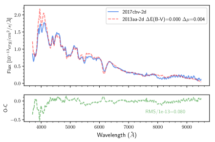
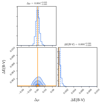
Figure 1: Left: Comparison of early time spectra of SN 2013aa and SN 2017cbv at -2 days before maximum light. Right: 1$\sigma$, 2$\sigma$ and 3$\sigma$ contours for the posterior probability distribution. The dashed veritcal values correspond to 1$\sigma$ error in each variable.

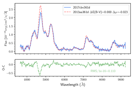
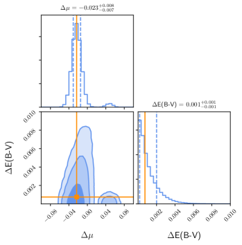
Figure 2: Left: Comparison of late-time spectra of SN 2013aa and SN 2017cbv at 361 days past maximum light. Right: As in Figure 1 but for the 361 days phase.

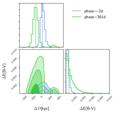
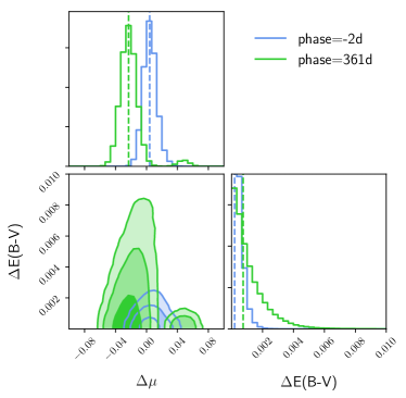
Figure 3: Comparison of the contours of posterior probability for the joint result from early and late time spectra of SN 2013aa and SN 2017cbv. It is given both in $\Delta$ kpc (left) and in $\Delta\mu$ (right)

Given the large amount of nebular data that are now being gathered, the galaxy NGC 5643 will eventually become an anchor for supernovae belonging to the class of twins of SN 2017cbv/SN 2013aa, hopefully reaching high enough $z$, where peculiar velocities do no longer prevent to reliably derive H₀.

3 The distance to NGC 7250

SN 2013dy in NGC 7250 has a decline rate similar to that of SN 2013aa and SN 2018cbv. We have found enough similarities to suggest that it belongs to the class of twins represented by SN 2017cbv and SN 2013aa. It follows an evolution identical to those SNe Ia. The characteristcs of this SNIa can be found in Table 3.

SN 2013dy was discovered a few hours after explosion. This circumstance made possible a very intense photometric and spectroscopic follow up of this SNIa (Pan et al. 2015). This supernova belongs to normal SNe Ia which can be fitted with a W7 type model with solar metallicity. (Nomoto, Thielemann & Yokoi 1984).

We went further looking for differences and similitudes with the two twin SNe Ia in NGC 5643. We were suprised to see the similarities in spectral evolution. We have selected three epochs to display this similitude: 2 days before maximum, 46 days after maximum and 333 days after maximum.

SN 2013dy is practically equal at late phases to SN 2017cbv (there are no spectra of SN 2013aa at that phase to allow a comparison). At very early phase it is similar to both SN 2017cbv and SN 2013aa though slightly redder. After maximum brightness is also identical to SN 2013aa.

Pan et al. (2015) show a comparison of the UV flux of SN 2013dy with that of SN 2011fe. The larger flux in SN 2013dy is consistent with a larger amount of ⁵⁶Ni than for SN 2011fe. So it is its longer rise to B maximum, which is 17.7 days in SN 2013dy against 17.6 days in SN 2011fe.

SN 2013dy had significant reddening. The reddening in the Galaxy is E(B-V)_MW $=$0.14 mag (Schlafly & Finkbeiner 2011), though there are indications that the total reddening might be higher with a possible lower R_V than 3.1. We will address this once we made our comparison of SN 2013dy with SN 2017cbv and SN 2013aa, those last ones reddened with a E(B-V)_MW$=$0.15 mag (Schlafly & Finkbeiner 2011).

Table 3: SN 2013dy

SN 2013dy
RA, DECa	22:18:17.599	+40:34:09.59
Discovery datea	$\dots$	2013-07-10
Phase (referred to maximum light)b	$\dots$	-18 days
Redshiftc	$\dots$	0.0039
E(B-V)MWd	$\dots$	0.15 mag
$m_{B}^{max}$ e	$\dots$	13.229$\pm$0.010 mag
$\Delta m(B)_{15}$ e	$\dots$	0.92$\pm$0.006 mag
Phases of the spectra used	$\dots$	-2, 46, 333 days

aCasper et al. (2013).	bZheng et al. (2013).	cSchneider et al. (1992).
dSchlafly & Finkbeiner (2011).	ePan et al. (2015).

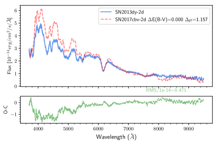
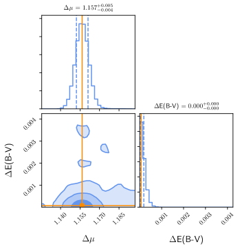
Figure 4: Left: Comparison of early time spectra of SN 2013dy and SN 2017cbv at -2 days before maximum light. Right: 1$\sigma$, 2$\sigma$, 3$\sigma$ contours for this epoch.

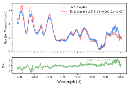
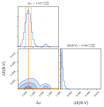
Figure 5: Left: Comparison of the spectra of SN 2013dy with SN 2013aa at 46 days past maximum light. Right: As above but for the 46 days phase.

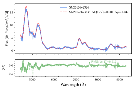
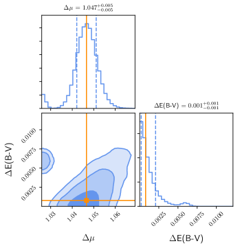
Figure 6: Left: Comparison of the spectrum of SN 2013dy and SN 2017cbv from late time spectra at 333 days. Right: Contours for the 333 days phase.

We see at early phase (2 days before maximum) (Figure 4) that SN 2013dy has a less steep spectrum (redder) than SN 2017cbv (and SN 2013aa). This is not due to reddening (as can be seen in later phases) but to an intrisic slightly different effective temperature of the spectrum. The spectral features are, though, equal between SN 2013dy and its twins at early phases. One might consider that this difference can be explained by an external factor, as there is an early blue excess both in spectra and the light curve in SN 2017cbv. It has been pointed out to the presence of a companion and to an explosion from a double detonation initated at the surface of the star for this supernova. In the case of SN 2013aa, early data are missing, so it is not possible to check whether there might have been indirect evidence for a companion. But SN 2013aa is identical to SN 2017cbv, so it might have arisen in a similar context.

From our purpose of distance determination, we exclude the earliest spectrum of SN 2013dy in our joint estimate of the distance of SN 2013dy, as there is a circumstancial factor only affecting the earliest epoch. The spectrum of SN 2013dy achieve just a few days later an amazing similarity to those of SN 2017cbv and SN 2013aa that last until the nebular phase. We obtain the derived distance to SN 2013dy from its comparison with phase 46 (Figure 5) and 333 days past maximum (Figure 6). The combined posterior distributions can be seen in Figure 7. The results on the distance are given in Table 4. One might note that $\Delta E(B-V)$ $=$ 0.0 $\pm$ 0.001. The Pearson correlation coefficient r of the variables $\Delta\mu$ and $\Delta E(B-V)$ for the 46 phase sample $=$ -0.025, and for the 333 phase $=$ 0.188, thus is very low. This might be explained by the fact that we are moving around a $\Delta E(B-V)$ very low. SN 2013dy has a similar total E(B-V) than its twins SN 2017cbv/SN 2013aa, and a reddening of E(B-V) $=$ 0.01 for SN 2013dy would arise in the host galaxy (E(B-V)_MW is 0.14 for SN 2013dy).

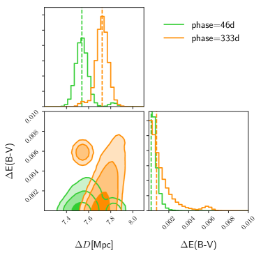
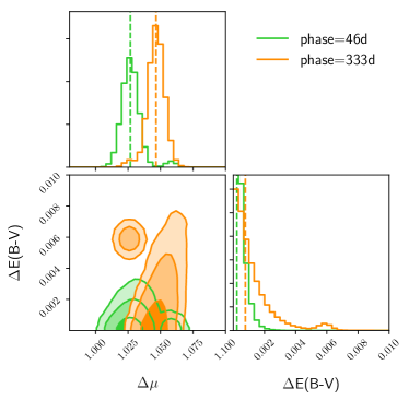
Figure 7: 1$\sigma$, 2$\sigma$, 3$\sigma$ regions from the comparison at 46 days after maximum and 333 days after maximum of SN 2013dy with its twins. Left: They are provided in $\Delta$d. Right: They are provided in $\Delta\mu$.

Table 4: The distance to NGC 7250

SN	Host	$\mu$	Error in $\mu$	Source
2013dy	NGC 7250	31.523	0.025 + 0.1∗	This work
2013dy	NGC 7250	31.628	0.125	Riess et al. (2022) (Cepheids)
Previous step in the ladder
2017cbv	NGC 5643	30.480	0.1	Hoyt et al. (2021)
2013aa	NGC 5643	30.480	0.1	Hoyt et al. (2021)
∗Error in the distance to NGC 5643.

4 The distance to NGC 2525

In this Section we proceed to use twin SNe Ia of other type. In particular, we are interested in the 2011fe–like group. SN 2018gv in NGC 2525 belongs to it. This allows us to determine the distance to this galaxy, for which only old, rather unrealistic Tully–Fisher distance measurements, plus a Cepheid measurement with substantial uncertainty are currently available.

We will now use the spectral twins method to estimate the distance to NGC 2525 through the comparison between SN 2011fe and SN 2018gv from early until nebular phases.

4.1 SN 2011fe in M101 as a reference

SN 2011fe was discovered, in the nearby spiral galaxy M101, in its very early phase and it was classified as a normal SN Ia (Nugent et al. 2011). It appears to have been discovered within a few hours after the explosion and this helped to put constraints on the progenitor system of the explosion (Nugent et al. 2011; Bloom et al. 2012). The pre-explosion Hubble Space Telescope image of the SN 2011fe location ruled out luminous red giants and almost all helium stars as the mass-donor companion of the exploding WD (Li et al. 2011). In addition, the early-time photometry of SN 2011fe (Bloom et al. 2012) set a limit to the initial radius of the primary star, R${}_{p}\leq 0.02R_{\odot}$, as well as a limit to the size of the companion star, R${}_{c}\leq 0.1R_{\odot}$. Tucker & Shappee (2023) have reported imaging follow-up of SN 2011fe during 11.5 yrs after discovery, that setting strong constraints to a possible single-degenerate progenitor systems. This result appears consistent with the lack of interaction with a non-degenerate companion in the Swift/UV light curves (Brown et al. 2012). The limits on post-impact donors by Tucker & Shappee (2023), together with constraints from pre-explosion imaging, early-time radio and X-ray observations, and nebular-phase spectroscopy, essentially rule out all formation channels for SN 2011fe invoking a non-degenerate donor star. This favours a double-degenerate progenitor for SN 2011fe.

At maximum light, the color was (B_max - V_max) = –0.07 $\pm$ 0.02 mag. The value of (B_max - V_max) being –0.12 mag in normal SNe Ia, this might mean that there is, in fact, some host galaxy extinction. With the removal of the Galactic component, E(B–V)_MW = 0.008 mag (Schlafly & Finkbeiner 2011), Pereira et al. (2013) estimated such reddening as E(B - V)_host = 0.026 $\pm$ 0.045 mag, by using the Lira relationship of the colors in the postmaximum phase, in close agreement with the 0.032 $\pm$ 0.045 mag obtained by Zhang et al. (2016). Tammann & Reindl (2011) obtained E(B–V)_host = 0.030 $\pm$ 0.060 mag from the B–V at the maximum of the light curves. The application of CMAGIC to SN 2011fe by Yang et al. (2020) gives a host galaxy extinction compatible with zero, E(B - V)_host = 0.0 $\pm$ 0.027 mag. Patat et al. (2013) studied, from multi–epoch high resolution spectroscopy of SN 2011fe, the reddening based on the absorption systems of Ca II and Na I towards the supernova. They inferred a host galaxy reddening from the equivalent width (EW) of Na I of E(B-V) $=$ 0.014 mag and they derive a Galactic reddening of E(B-V)_MW $=$ 0.01 mag (similar to tha from Schlafly & Finkbeiner 2011). So, there is a total E(B-V)$=$ 0.024 mag from this last reference. We adopt such value as a most accurate guess, though the absolute value is not something needed for the application of the method. The reddening relative to its twin will be determined by the MCMC.

Concerning the luminosity decline parameter of SN 2011fe, Burns et al (2023, private communication) measured a $\Delta m_{15}(B)$ = 1.07$\pm$0.006 mag. The basic data for SN 2011fe are given in Table 5.

The derived Fe abundance in the outermost layers of the ejecta is consistent with the metallicity at the SN site in M101 ($\sim$ 0.5 Z_⊙: Mazzali et al. 2015). This produces differences in the spectrum as compared with the W7 model, which has solar metallicity, with higher UV flux and affecting as well the blue spectrum at early phases. At post–maximum phases, save differences in the UV part of the spectrum, the rest of the wavelemgths converge to a model based on solar metallicity such as W7. This makes twin pairing with the SN 2011fe-like SNe to be better in the optical and improving after maximum, when the photosphere has receded to the SN core. Several modeling approaches give, for SN 2011fe, an amount of ⁵⁶Ni of 0.5 M_⊙ synthesized in the explosion. Pereira et al. (2013), from the bolometric light curve of the supernova obtain 0.53 $\pm$ 0.11 M_⊙ of ⁵⁶Ni. Zhang et al (2016), using as well the bolometric light curve, estimate around $\sim$ 0.57 M_⊙ of ⁵⁶Ni. Mazzali et al. (2015) derived a mass of ⁵⁶Ni $\sim$ 0.47 $\pm$ 0.05 M_⊙ and a stable iron mass of $\sim$ 0.23 $\pm$ 0.03 M_⊙ for SN 2011fe, based on modeling of the nebular spectra. A centrally ignited SN Ia in a Chandrasekhar-mass model similar to W7 (with production of a slghtly lower mass of ⁵⁶Ni) seems to agree with the chemistry of this SN.

Since SN 2011fe turns to be a kind of “template” for a class of normal SNe Ia, this nearby supernova teaches us the level of ⁵⁶Ni for that class.

A distance to M101 (the host galaxy of SN 2011fe) as that provided by the TRGB method is also in good agreement with the observed flux of the SN. Here, however, we basically deal with the difference of distances between SN 2011fe and SN 2018gv, although SN 2011fe being the anchor (the previous step of reference in the distance ladder) here, its distance enters in the final result.

Table 5: SN 2011fe and SN 2018gv

SN 2011fe
RA, DECa	14:03:05.810	+54:16:25.39
Discovery datea	$\dots$	2011-08-24
Phase (referred to maximum light)b	$\dots$	-20 days
Redshiftc	$\dots$	0.0012
E(B-V)MWd	$\dots$	0.008 mag
$m_{B}^{max}$ e	$\dots$	9.983$\pm$0.015 mag
$\Delta m(B)_{15}$ e	$\dots$	1.07$\pm$0.06
Stretch factor $s_{BV}^{D}$b	$\dots$	0.919$\pm$0.004
Phases of the spectra used	$\dots$	9, 289, 344 days
SN 2018gv
RA, DECf	08:05:34.580	-11:26:16.87
Discovery dateg	$\dots$	2018-01-15
Phase (referred to maximum light)f	$\dots$	-16 days
Redshiftf	$\dots$	0.0053
E(B-V)MWd	$\dots$	0.008 mag
$m_{B}^{max}$ e	$\dots$	12.8$\pm$0.015 mag
$\Delta m(B)_{15}$f	$\dots$	0.983$\pm$ 0.15
Stretch factor $s_{BV}^{D}$b	$\dots$	0.937$\pm$0.031
Phases of the spectra used	$\dots$	9, 289, 344 days

aWaagen (2011).	bRichmond & Smith (2012)	cCenko et al. (2011)
dSchlafly & Finkbeiner (2011).	eBurns (private communication, (2023).	fYang et al. 2020.
gItagaki (2020).

4.2 2018gv

SN 2018 gv is a SN 2011fe-like supernova. The explosion was fairly symmetric and the spectra were similar all along the different phases. The supernova was discovered on 2018-01-15 by K. Itagaki in the outskirts of the host galaxy NGC 2525 (Itagaki 2018), a barred spiral galaxy at $z$ = 0.00527 (de Vaucouleurs et al. 1991).

The Galactic reddening in the direction of SN 2018gv is E(B-V)_MW = 0.051 mag, according to the extinction map by Schlafly & Finkbeiner (2011). It is appreciably higher than that of SN 2011fe. The host galaxy reddening should be very low, given the position of SN 2018gv in the outskirts of its host galaxy. The test for reddening from the Lira relation gives that same amount, for the total reddening, as for just the Galactic one. The application of the CMAGIC method in Yang et al. (2020) gives a host reddening of E(B-V)_host = 0.028 $\pm$ 0.027 mag, thus being compatible with zero.

The basic information on SN 2018gv can be found in Table 5. The early-time spectra of SN 2018gv show strong similarity in most respects with those of the normal Type Ia SN 2011fe (Yang et al. 2020). These authors demonstrate that SN 2018gv resembles SN 2011fe for the first 100 days and exhibits a low Si II velocity gradient in the days after peak brightness. The observation of low continuum polarization overlaid by significant line polarization would be inconsistent with an asymmetric explosion. They suggest an amount of ⁵⁶Ni of 0.56 $\pm$ 0.08 $M_{\odot}$ from the bolometric light curve (Yang et al. 2020). Graham et al (2022) show the even stronger late-time similarity between SN 2011fe and SN 2018gv. They fully deserve to be named “nebular twins’: at the same phases in the nebular evolution they have extremely similar spectra. For the application of our method, the likeness of the spectra of twin SNe Ia can not just consist of the fact that two nebular spectra might be, at some particular close times, similar. It should happen at exactly the same nebular stages. Being similar through the whole nebular phase indicates closely resembling Ni cores, which are the sources of the luminosity of the supernovae at those epochs

As stated above, the two SNe Ia are very similar at early times, and that mostly persists until the nebular phase, with a few noticeable differences, however. So, for instance, the line width measurements suggest a slight difference in central density, though both densities are high enough to form stable Fe-group elements in the innermost regions of the core.

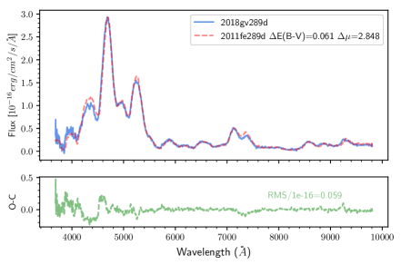
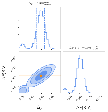
Figure 8: Left: Spectra of the twins SN 2011fe and SN 2018gv at exactly the same phase of 289 days past maximum light. Right: Corner plot as in previous figures but for SN 2018gv at 289 days-

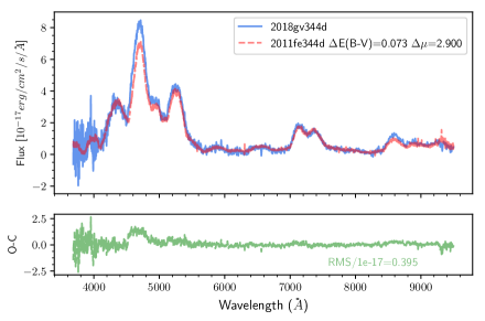
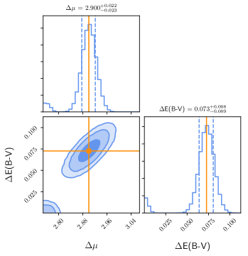
Figure 9: Left: Spectra of the twins SN 2011fe and SN 2018gv at exactly the same phase of 344 days past maximum light. Right: As above but for 344 days past maximum.

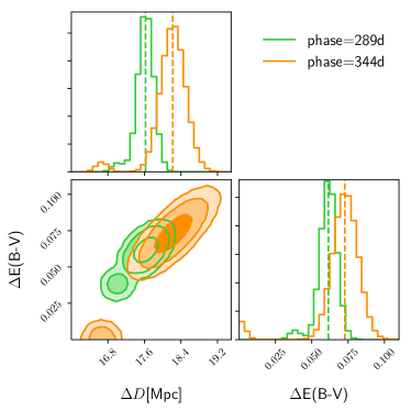
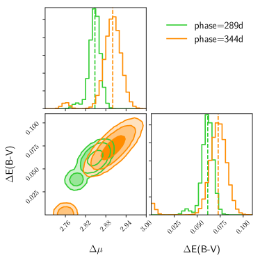
Figure 10: Joint confidence regions from the comparison at 289 days after maximum and 344 days after maximum of SN 2018gv and SN 2011fe. Left: They are provided in $\Delta$d. Right: They are provided in $\Delta\mu$.

4.3 $\Delta E(B-V)$ and distance

SN 2011fe and SN 2018gv were not heavily obscured by dust, as they occurred in the outskirts of their host galaxies. The Galactic redenning towards their direction has been measured, as stated above, by Schlafly & Finkbeiner (2011) for both SNe Ia.

To compare the spectra of the two SNe Ia, we have dereddened and deredshifted them both. 2011fe has been dereddened by 0.024 and SN 2018gv by 0.05 mag. The quantity $\Delta$ E(B - V) is the amount of reddening that we would need to add to SN 2018gv to get the best fit between the spectra of the two SNe. The result, $\Delta$ E(B - V), indicates whether E(B–V) might be higher in SN 2018gv than in SN 2011fe.

The results concerning the distance are, as already stressed, a relative distance between SN 2018gv and SN 2011fe. SN 2011fe, being one of the nearest and best observed SNe Ia and a prototype “normal” SN Ia, is our first SN Ia that can work as an anchor for the extragalactic distance scale.

We search for the best match between SN2018gv and SN2011fe using only two free parameters, the reddening value difference, $\Delta$ E(B-V), and modulus difference $\Delta\mu$. We have used the similarity between the spectra of SN2011fe and SN2018gv at three different phases and we perform a fit using the likelihood function defined in [1] (Section 3).

We run again the Markov Chain Monte Carlo with 32 walkers and 10,000 steps each, implemented in EMCEE (Foreman-Mackey et al. 2013), sufficient to get a statistically significant result. In each MCMC sample our code is able to deredden the reference spectrum (that of SN 2011fe) with a given value of E(B-V) and size the parameters $(\Delta E(B-V)$ and $\Delta\mu$), relative to SN 2018gv. We adopted uniform priors on the $\Delta D$ ($\mathcal{U}[15,21]$ Mpc) and reddening $\Delta E(B-V)(\mathcal{U}[0.0,0.8]$ mag). In Figure 8 and Figure 9, we show the posterior distributions for two different epochs and in Figure 10 the one corresponding to the combined regions. At the end, we found that the early spectrum we were going to use was not reliable as there were different reductions for the same epoch with incompatible spectral shape in the WISeREP (see the above database to check this point). We should note that here the Pearson correlation coefficient r is significantly higher than for SN 2013dy, manifesting the obvious implications that a change of $\Delta(E-V)$ has in $\Delta\mu$ in this nearly identical spectra. As we see, the results favour $\Delta E(B-V)$ = 0.061 ${}^{+0.004}_{-0.005}$ mag more in SN 2018gv than in SN 2011fe, and $\Delta\mu$ = 2.848 ${}^{+0.011}_{-0.013}$ mag. The distance factor between SN 2018gv and SN 2011fe is 3.711: $D_{2018gv}=3.711\times D_{2011fe}$. Those are sumarized in Table 6.

4.4 M101

M101 is very nearby but nevertheless its distance measured by Cepheids (SH0ES) differs from that obtained through TRGB. In the case of the use of Cepheids, it is remarkable that in Riess et al. (2016) the distance modulus was 29.135$\pm$0.045 mag and in Riess et al. (2022) a reanalysis of the data gave 29.194 $\pm$ 0.039 mag, which place M101 at practically 7 Mpc. In fact, the value in Riess et al (2022) makes the absolute magnitude of SN 2011fe a significantly more luminous SN Ia than what has been found by most authors. The TRGB value by Beaton et al. (2019) seems a much better choice to place SN 2011fe in its luminosity rank.

It has been mentioned (Tammann & Reindl 2011) that the problem of M101 is that the Cepheids in an outer, metal-poor field (Kelson et al. 1996) and in two inner, metal-rich fields (Shappee & Stanek 2011), yield discordant distances.

Table 6: Distance moduli for SN 2018gv and SN 2011fe

2018gv	$\mu$ = 32.051$\pm$0.099	Cepheids1
2018gv	$\mu$ = 31.912$\pm$0.091	This work
2011fe	$\mu$ = 29.135$\pm$ 0.045	Cepheids2
2011fe	$\mu$ = 29.194$\pm$0.039	Cepheids1
2011fe	$\mu$ = 29.07$\pm$0.09	Tip of the Red Giant Branch3

1Riess et al. (2022)	2 Riess et al. (2016).
3Freedman et al. (2019).

The TRGB distance to M101 value in Freedman et al (2019) is actually coming from Beaton et al. (2019). This distance modulus is $\mu$ = 29.07 $\pm$ 0.04 (stat) $\pm$ 0.05 (sys) mag, which corresponds to a physical distance $D$ = 6.52 $\pm$ 0.12 (stat) $\pm$ 0.15 (sys) Mpc.

The final distance to NGC 2525 obtained by the present method is mostly affected, now, by the uncertainty on the distance to M101. Otherwise, the error would be small. So, we obtain $\mu$ = 31.912 $\pm$ 0.0912 mag, adopting a distance modulus for M101 of $\mu$ $=$ 29.07 $\pm$ 0.09 mag (Beaton et sl. 2019). $\Delta\mu$ is 2.848${}^{+0.0011}_{-0.0013}$ mag in our results (see Figures 8 and 9). The largest uncertainty thus comes from the distance to M101, with an error of 0.09 mag in $\mu$.

The determination by SH0ES of the distance to NGC 2525 corresponds to a distance modulus of $\mu$ = 32.051 $\pm$ 0.099 mag, which is a distance of 25.716${}^{+1.199}_{-1.14}$ Mpc. If we take the SH0ES distance modulus of M101 of 29.135$\pm$0.045 mag, the distance factor between SN 2018gv and SN 2011fe becomes 3.831.

In our determination of the distance to NGC 2525, the distance modulus obtained corresponds to a distance of 24.121${}^{+1.033}_{-0.989}$ Mpc when adopting the distance modulus for M101 of Beaton et al. (2019), which corresponds to a distance of 6.516${}^{+0.276}_{-0.264}$ Mpc. The distance factor of SN 2018gv in relation to SN 2011fe is 3.71, then.

5 Discussion

While the use of twins has been proved to be very useful for distance determinations, pairing SNe Ia which are not true twins can lead to errors in distance estimates. A good first order guide is to explore only SNe Ia within similar stretch values s_BV. Then, within a similar strech family, one can compare the spectra at various phases, as we have done here. We have looked to twins of the SN 2013aa/SN 2017cbv class, as well as to the SN2011fe class.

How to size the difference in between SNe Ia twin classes?. If we placed 2013aa at the distance of 6.5 Mpc for SN 2011fe, we find a factor of 1.46 of difference in flux level. If we wrongly took SN 2013aa for a twin of SN 2011fe, the error in distance would be by a factor of 1.208 (see Figure 11).

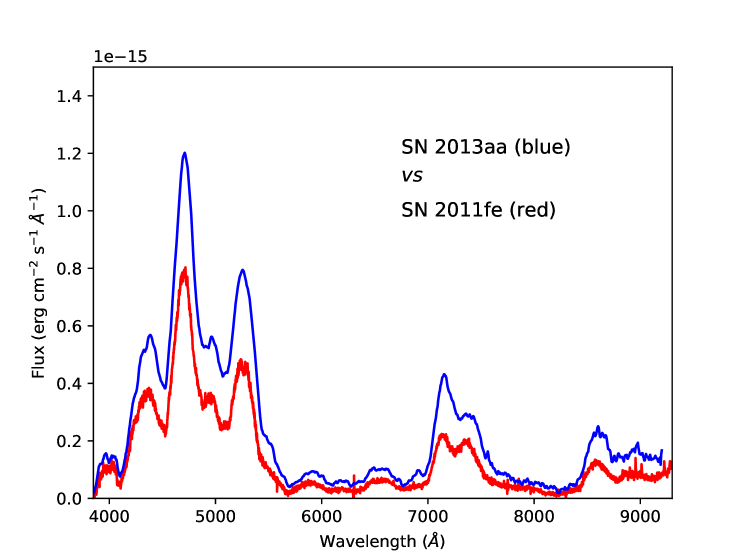
Figure 11: Comparison of the spectra of SN 2013aa and SN 2011fe at the same phase. The reddening of SN 2011fe has been placed at E(B-V)$=$ 0.15 to compare it with SN2013aa.

There is a lack of the spectral line of stable Ni in SN 2013aa, which indicates that the WD ignited at a lower central density than in SN 2011fe there. The line due to the presence of stable Ni isotopes points to a start of the ignition at high densities, in SN 2011fe. Both SN 2011fe and SN2018gv underwent explosive burning at a higher density than SN 2017cbv and SN 2013aa. The mismatch between them is seen at both early and late phases. In fact, SN 2013aa and SN 2017cbv synthesized about 0.23 M_⊙ more ⁵⁶Ni than the pair SN 2011fe and SN 2018gv, as suggested by the overall higher flux. This is corroborated by previous studies (Jacobson-Galán et al. 2018) suggesting 0.732 $\pm$ 0.151 M_⊙ of ⁵⁶Ni in SN 2013aa.

5.1 The whole SNe Ia calibrating sample

By looking at the nebular spectra of the sample of SNe Ia in the calibrating samples of galaxies of TRGB (18 SNe Ia in 15 galaxies) of Freedman et al. (2019), and in the calibrating sample of 42 SNe Ia in 37 galaxy hosts of Riess et al. (2021), we have twins of SN 2011fe, as well as twins of SN 2017cbv/2013aa. There is also the class of SNe Ia with light echos, which can be close to SN 2011fe or to SN 1991T in those calibrating samples. In fact SN 1991T had an echo. There seems to be as well a class represented by SN 2012cg with its twin SN2009ig, which show evidence of interaction with a non-degenerate companion and produce around 0.8 M_⊙ of ⁵⁶Ni. The lack of strong lines of stable Ni points to ignition at a lower density than in SN 2011fe, there.

In general, in those SNe Ia lists, there is a range of SNe Ia which have synthesized different amounts of ⁵⁶Ni (from 0.4 to 0.8 M_⊙) and have undergone thermonuclear burning at different densities. In addition, SNe Ia do have peculiarities such as evidence for an early interaction with a supernova companion, or the presence of an echo at late times.

For the first time, a long coverage of a SN Ia at the nebular phase has been obtained, from 400 days to 1000 days in the case of SN 2011fe (Tucker et al 2022). We have seen clearly how the ionization stage changes significantly along this time, for this normal SN Ia. But even from 200 to 460 days the level of ionization of Fe⁺ and Fe⁺⁺ undergoes significant change.

A dense grid of nebular spectra of SNe Ia would facilitate the twins classification. The use of this database should enable comparison of spectra of different supernovae at similar dates. The wide use of significant different phases, as done often nowadays, should be avoided as it affects the evaluation of the masses of NSE nuclides synthesized in the explosion. The abundances of stable NSE nuclides are indicators of the densities at which the WDs explode and they also give clues about the mechanism involved in the explosion. But, for the present case, the overall flux of the elements from the decay of ⁵⁶Ni synthesized in the explosion make the overall flux of the spectra at late times, therefore affecting any distance determination.

Reliable distances can be obtained by pairing the twins until the nebular phase, once proper flux calibration and choice of similar phases are done. Including the nebular phase can prevent errors made when matching the very early phases, at which times different interactions with circumstellar material or possible heating from a companion would produce differences in the spectra.

The distance to M101 from Beaton et al. (2019) using the TRGB method is consistent with SN 2011fe having synthesized 0.5 M_⊙ of ⁵⁶Ni, as most authors have found (see Appendix as well). It will be worth to obtain a well established distance to this nearby galaxy from all methods, as it hosts one of the most prototypical and well studied SNIa, SN 2011fe.

The difference between SN 2011fe and the SN 2017cbv/2013aa suggests that that NGC 5643 is at $\mu$ = 30.47 $\pm$ 0.1 mag and NGC 7520 is at $\Delta d$ = 7.7 $\pm$ 0.1 Mpc ($\Delta\mu$ = 1.055 $\pm$ 0.025 mag ) away from NGC 5643, thus at 31.523 $\pm$ 0.111 (error mostly due to that associated to the distance to NGC 5642). The value is compatibe with the one derived by the Cepheids: 31.628 $\pm$ 0.125 from SH0ES (Riess et al. 2022).

The method has been applied as well to the twins of SN 2011fe in M101 and SN 2018gv in NGC 2525. This has allowed to determine a distance of 24.121 ${}^{+1.033}_{-0.989}$ Mpc to NGC 2525. The value reported by Riess et al is 25.716 Mpc ${}^{+1.199}_{-1.14}$ Mpc. The result is compatible with that from the Cepheids, though it does not align well with the extreme distance $\sim$ 27 Mpc in the upper edge of the uncertainty towards NGC 2525 obtained from the Cepheids. The SH0ES collaboration measurement places SN 2018gv at a relative distance factor $\sim$ 3.8 times that of SN 2011fe, while we favor a factor $\sim$ 3.7 times.

It seems clear that twins followed until the nebular phase can establish the distance ladder in the epoch of large surveys such as the LSST. The infrared part of the nebular spectra of SNe Ia will soon become widely available, from programs already approved for the JWST. The infrared will reveal further differences among SNe Ia in that part of the spectra, thus helping in the twin classification.

6 CONCLUSIONS

It has been proved here that comparison of twin SNe Ia can provide a robust way to establish the extragalactic distance ladder. The method has been applied to the twins in the galaxy NGC 5643: SN 2013aa and SN 2017cbv. The comparison using spectra before maximum and at the nebular phase shows that the error in the distance determination is of $\Delta\mu$ $\sim$ 0.004 mag.

Distances obtained here for NGC 7520 and NGC 2525 are consistent with those obtained by Riess et al (2022), while we can not compare them with the TRGB method since it has not been applied to these galaxies. The value of the distance to NGC 5643 (Hoyt et al. 2021) is in good accordance with the one derived by the SNe Ia in this paper, but not with that presented by Riess et al. (2022). The difference of $\mu_{Cepheids}$ $=$ 30.57 $\pm$ 0.05 mag versus $\mu_{TRGB}$ $=$ 30.48$\pm$0.1 mag by Hoyt et al. (2021) seems larger than the usual 0.05 mag ( $\Delta\mu$ $\sim$ 0.1 ), leaving aside the errors. If one takes into account that NGC 5643 is a nearby galaxy, the difference calls for a revision, though within errors, the distances are compatible.

In the near future, we plan to complete the check for the galaxy sample measured by Cepheids and TRGB published so far by applying our method. But we want to go to distant galaxies as a priority, as we suspect that most of the difference in the H₀ value from Cepheids and from TRGBs might arise from different treatments of the peculiar velocities.

The way to evade the problem of peculiar velocities to obtain H₀ is to use SNe Ia twins in galaxies of the Coma cluster or any galaxy at z $\sim$ 0.02–0.03, already in the Hubble flow. We would like to extend the method of the twin distance determinations to SNe Ia already in the Hubble flow obtaining spectra not only near maximum, but also well into the epochs where SNe Ia show the diversity of the inner core, specially the Fe-peak elements and ⁵⁶Ni–rich innermost layers. That should be achievable with the JWST or the ELT.

The authors would like to thank Melissa Graham and Chris Burns for generously providing spectra used in the present paper. This work has made use as well of spectra from the Weizmann Interactive Supernova data REPository (WISeREP). Gaia DR3 photometry was used in the calibration of SN 2018gv/Gaia18bat data. We acknowledge ESA Gaia, DPAC and the Photometric Science Alerts Team (http://gsaweb.ast.cam.ac.uk/alerts). PR-L would like to thank Michael Weiler and Josep Manel Carrasco from the Gaia–ICCUB team for their help in crosschecking the calibration of the spectra of SN 2018gv at late phases. PR-L also acknowledges support from grant PID2021-123528NB-I00, from the the Spanish Ministry of Science and Innovation (MICINN). JIGH acknowledges financial support from MICINN grant PID2020-117493GB-I00.

BIBLIOGRAPHY

Beaton, R.L., Seibert, M., Hatt, D., et al. 2019, ApJ, 885, 141

Bernal, J.L., Verde, L., & Riess, A.G. 2016, JCAP, 10, 019

Blakeslee, J.P., Jensen, J.B., Ma, C.-P., Milne, P.A., & Greene, J.E. 2021, ApJ, 911, 65

Bloom, J.S., Kasen, D., Sen, K.J., et al. 2012, ApJL, 144, L17

Boone, K., Fakhouri, H., Aldering, G.A., et al. 2016, AAS Meeting, 227, 237.10

Brown, P.J., Dawson, K.S., Harris, D.W., et al. 2012, ApJ, 749, 18

Burke, J., Howell, D.A., Sand, D.J., et al. 2022, arXiv:220707681

Burns, C.R., Stritzinger, M., Phillips, M.M., et al. 2014, ApJ, 789, 32

Burns, C.R., Ashall, C., Contreras, C., et al. 2020, ApJ, 895, 118

Casper, C., Zheng, W., Li, W., et al. 2013, CBET, 3588

Cenko, S.B., Thomas, R.C., Nugent, P.E., Kandreshoff, M., Filippenko, A.V., & Silverman, J.M. 2011, ATel, 3583, 1

de Vaucouleurs, G., de Vaucouleurs, A., Corwin, H.G., Buta, R.J., Paturel, G., & Fouque, P. 1991, Third Reference Catalogue of Bright Galaxies, Vol. 1 (Springer, New York)

Di Valentino, E., Melchiorri, A., & Silk, J. 2021, ApJL, 908, L9

Efstathiou, G., Rosenberg, E., & Poulin, V. 2023, arXiv:2311.00524

Fakhouri, H.K., Boone, K., Aldering, G., et al. 2015, ApJ, 815, 58

Foreman-Mackey, D., Hoog, D.W., Lang, D., & Gooodman, J. 2013, PASP, 125, 300

Freedman, W.L., Madore, B.F., Hatt, D., et al. 2019, ApJ, 882, 34

Freedman, W.L. 2021, ApJ, 919, 16

Freedman, W.L., & Madore, B.F. 2023, JCAP, 11, 050

Gelman, A., Roberts, G.O., & Gilks, W. 1996, Bayesian Statistics,

Goodman, J., & Weare, J. 2010, Communications in Applied Mathematics and Computational Science, 5, 65

Graham, M.L., Kennedy, T.D., Kumar, S., et al. 2022, MNRAS, 511, 3682

Guy, J., Astier, P., Nobili, S., Regnault, N., & Pain, R. 2005, A&A, 443, 781

Hoyt, T., Beaton, R.L., Freedman, W.L., et al. 2021, ApJ, 915, 34

Hamuy, M., Phillips, M.M., Maza, J.; Suntzeff, N.B., Schommer, R.A., & Avilés, R. 1995, AJ, 109, 1

Huang, C.D., Yuan, W., Riess, A.G., et al. 2023, arXiv:2312.08423

Itagaki, K. 2018, TNSTR, 57, 1

Jacobson-Galan, V.W., Dimitriadis, G., Foley, R.J., & Kirpatrick, C.D. 2018, ApJ, 857, 88

Jha, S., Riess, A.G., & Kirshner, R.P. 2007, ApJ, 659, 122

Kelson, D.D., Illingworth, G.D., Freedman, W.L., et al. 1996, ApJ, 463, 26

Kenworthy, W.D., Riess, A.G., Scolnic, D., et al. 2022, ApJ, 935, 83

Khetan, N., Izzo, L., Branchesi, M., et al. 2021, A&A, 647, A72

Li, W., Bloom, J.S., Podsiadlowski, P., et al. 2011, Natur, 480, 348

Livne, E., & Arnett, D. 1995, ApJ, 452, 62

Mazzali, P.A., Sullivan, M., Filippenko, A.V., et al. 2015, MNRAS, 450, 2631

Murakami, Y.S., Riess, A.G., Stahl, B.E., et al. 2023, JCAP, 11, 046

Nomoto, K., Thielemann, F.-K., & Yokoi, K. 1984, ApJ, 286, 644

Nugent, P.E., Sullivan, M., Cenko, S.B., et al. 2011, Natur, 480, 344

Pan, Y.C., Foley, R.J., Kromer, M., et al. 2015, MNRAS, 452, 4307

Parrent, J.T., Sand, D., Valento, M., Graham, D.A., & Howell, D.A. 2013, ATel, 4817, 1

Patat, F., Cordiner, M. A., Cox, N. L. J., et al. 2013, A&A, 549, A62

Pereira, R., Thomas, R.C., Aldering, G., et al. 2013, A&A, 554, A27

Perlmutter, S., Aldering, G., Goldhaber, G., et al. 1999, ApJ, 517, 565

Phillips, M.M. 1993, ApJL, 413, L105

Phillips, M.M., Lira, P., Suntzeff, N.B., et el. 1999, AJ, 118, 1766

Planck Collaboration 2020, A&A, 641, A6

Richmond, M.W., & Smith, H.A. 2012, JAVSO, 40, 872

Riess, A.G., Press, W.H., & Kirshner, R.P. 1996, ApJ, 473, 88

Riess, A.G., Filippenko, A.V., Challis, P., et al. 1998, AJ, 116, 1009

Riess, A.G., Casertano, S., Anderson, J., et al. 2014 (M101), ApJ, 785, 161

Riess, A.G., Macri, L.M., Hoffmann, S.L., et al. 2016, ApJ, 826, 56

Riess, A.G., Casertano, S., Yuan, W., et al. 2019, ApJ, 876, 85

Riess, A.G., Casertano, S., Yuan, W., et al. 2021, ApJL, 908, L6

Riess, A.G., Yuan, W., Macri, L.M., et al. 2022, ApJ, 934, L7

Rubin, D., Aldering, G., Betoule, M., et al. 2023, arXiv:2311.12098

Ruiz–Lapuente, P., & Lucy, L.B., 1992 ApJ, 400, 127

Ruiz–Lapuente, P. 1996, ApJ, 465, L83

Schlafly, E.F., & Finkbeiner, D.P. 2011, ApJ, 737, 103

Schneider, S.E., Thuan, T.X., Mangum, J.G., & Miller, J. 1992, ApJS, 81, 5

Scolnic, D., Brout, D., Carr, A., et al. 2022, ApJ, 938, 113

Shappee, B.J., & Stanek, K.Z. 2011, ApJ, 733, 124

Shingles, L.J., Sim, S.A., Kromer, M., et al. 2020, MNRAS, 492, 2029

Shingles, L.J., Flors, A., Sim, S.A, et al. 2022, MNRAS, 512, 6150

Stahl, B.E., Zheng, W., de Jaeger, T., et al. 2020, MNRAS, 492, 4325

Stritzinger, M., Hamuy, M., Suntzeff, N.B., et al. 2002, AJ, 124, 2100

Suntzeff, N.B., Hamuy, M., Martin, G., Goomez, A., & Gonzalez, R. 1988, AJ, 96, 1864

Tammann, G.A., & Reindl, B. 2011, arXiv:1112.0439

Tartaglia, R., Sand, D., Wyatt, S., et al. 2017, ATel, 4158, 1

Tucker, M.A., Shappee, B.J., Kochanek, C.S., et al. 2022, MNRAS, 517, 4119

Tucker, M.A., & Shappee, B.J. 2023, arXiv:2308.08599

Waagen, E.O. 2011, AAN, 446, 1

Waagen, E.O. 2013, AAN, 479, 1

Wilk, K.D., Hiller, D.J., & Dessart, L. 2018, MNRAS, 474, 3187

Woosley S. E. & Weaver T. A.. 1994, in Supernovae, Les Houches Session IV, ed. Bludman S. A., Mochkovitch R., Zinn-Justin J. (Amsterdam–North–Holland), pg. 63

Yang, Y., Hoeflich, P., Baade, D., et al. 2020, ApJ, 902, 46

Zhai, Q., Zhang, J.-J., Wang, X.F., et al. 2016, AJ, 151, 125

Zhang, K., Wang, X., Zhang, J., et al. 2016, ApJ, 820, 677

Zheng, W., Silverman, J.M., Filippenko, A.V., et al. 2013, ApJL, 788, L15

APPENDIX

A. Theoretical anchor for SN 2011fe in M101

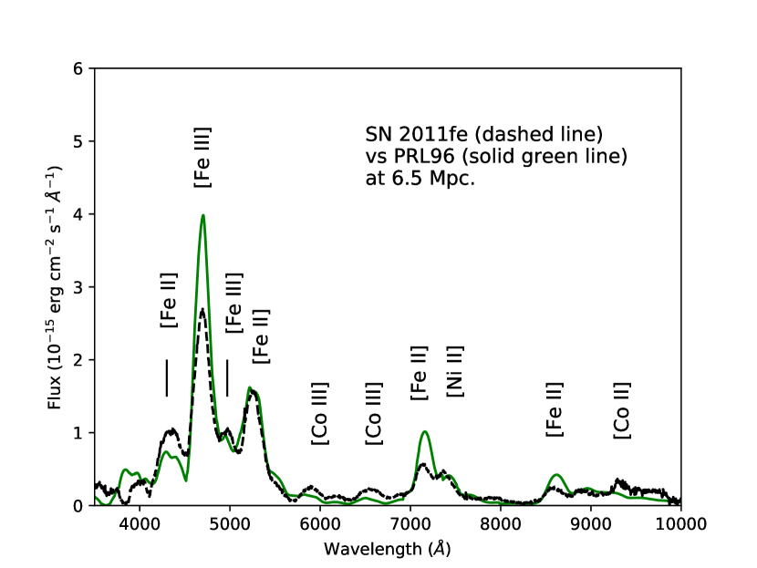
Figure 12: A distance of 6.5 Mpc seems compatible with late time spectrum of SN 2011fe. Here a comparison is made with a theoretical spectrum with a ⁵⁶Ni mass of 0.5 M$\odot$ of the W7 class obtained with the code explained in Ruiz–Lapuente (1996).

At late phases, the population of the energy levels of the ions present in the supernova ejecta is out of LTE because the density of the electrons responsible for collisionally exciting the lines is lower than the critical density for the corresponding transitions. Forbidden emission can be exploited here, since such emission from iron ions (especially Fe⁺) trace very well the electron density (n_e) of the supernova ejecta “nebula”. This fine sensor of the density profile can help to probe the mass of the exploding white dwarf and its kinetic energy. A clear diagnostic of low n_e comes from the emission at $\lambda$5200 Å, $\lambda$4300 Å, and $\lambda$5000 Å. These emissions are due to Fe⁺ a⁴F-b⁴P and a⁴F-a⁴H transitions, whose lower energy terms can be significantly depopulated if n_e is low. This ratio becomes a diagnostic of ejected mass. If lower masses give on average lower collisional excitation rates for those forbidden transitions, the rates decrease significantly. Another interesting ratio of [Fe II] is that of a⁴F-b⁴P to a⁴F-a⁴P, with emissions at $\lambda$5262 and $\lambda$8617 Å, though there are emissions at around 8600 Å from other elements that can prevent the discrimination. In any case, these [Fe II] lines at long wavelenghth do inform on how reddened the SN Ia is. They provide an internal estimate of reddening.

The second aspect relative to the amount of ⁵⁶Ni is that it impacts the degree of ionization and electron temperature T_e of the ejecta, which are kept warm by the thermalization of the $\gamma$-rays and positrons (e⁺) from the decay of ⁵⁶Co (coming from ⁵⁶Ni) into ⁵⁶Fe. While the emissivity of the different forbidden transitions of Fe⁺ keeps track of the electron density profile of the supernova, the ratio Fe⁺ to Fe⁺⁺ gives information on T_e and the ionization of the ejecta. Since there is a large number of forbidden lines over the wavelength range at which SNe Ia are observed, there is also complementary information to obtain an internal estimate of the reddening. A good description of the ionization degree of the ejecta depends on the ionization treatment in the radiation transport code, and on factors that need evaluation, such as trapping of the positron energy, among others. A feature inherent to the density of the ejecta is that the ionization stage is kept high (more Fe III in detriment of Fe II) when the density is low and the recombination rates decrease.

A fit with a theoretical spectrum is shown in Figure 12 to illustrate the ions present and dominating the emission of SN 2011fe at a late phase.

There is a general agreement, among different authors using different codes, that sub-Chandra explosion models tend to produce overionized ejecta (Ruiz-Lapuente 1996; Mazzali et al. 2015; Wilk et al 2018, Shingles et al. 2020), though the more recent denser sub–Chandrasekhar models seeem to fit as well as Chandrasekhar models the spectra of normal SNe Ia. In general, there is an overionization in the theoretical spectra calculated for all the models with the available codes and that is being currently addressed (see Shingles et al 2022). An internal test at the nebular phase showed that the R96 code and the ARTIS code gave the same overall flux level of the nebular spectra for W7 model amongst others.

Due to the limitations to achieve a perfect fit, and the need of being extremely precise in the distance derived with spectra, a decision to proceed towards a purely empirical approach was made. This has proved to be very successful.

B. Historical considerations

In the 90’s, the use of theoretical models to infer basic properties of the SNe Ia from spectra taken at late times was proposed (see Ruiz–Lapuente 1996; Ruiz–Lapuente & Lucy 1992). The idea was to obtain at the same time the ⁵⁶Ni mass, the reddening and the distance to the SN. Using this method, Ruiz Lapuente (1996) derived, for a reduced sample of SNe Ia, a value of the Hubble constant of H₀ = 68 $\pm$ 6 (statistical) $\pm$ 7 (systematic) km s^-1 Mpc^-1. The procedure was first to measure distances to the SNe Ia, then obtain their absolute B magnitude at peak brightness and derive a fiducial absolute magnitude M_B for the SNe Ia sample. Then, this one was tied to to a H₀ value as in Hamuy et al. (1995):

$${\rm log}H_{0}=0.2\{M^{B}_{\rm MAX}-1.624(\pm 0.582)[\Delta m_{15}(B)-1.1]+28.296(\pm 0.080)\}$$ (3)

Such calibration has changed dramatically since the 90’s. Now the Phillips relation includes terms in higher orders of $[\Delta m_{15}(B)-1.1]$. The derivation of H₀ relies on the connection between the second and third rung in the cosmic distance ladder, i.e from SNe Ia which are not in the Hubble flow (with z well below 0.1) and those which are already in the Hubble flow. The process used by most collaborations still relies in obtaining a fiducial absolute magnitude in B of the SNe Ia at peak, M${}^{0}_{B}$, in the local SNe Ia sample. However, such derivation needs corrections from extinction, variations of colors at peak maximum brightness in the sample, dependency with the host galaxy. In addition. to place them in the Hubble flow a reliable intercept with the SNe Ia in the Hubble flow is required. Given the complexity of this route, it is not strange to find that M${}^{0}_{B}$ varies amongst publications.

We can skip intermediate paths in this project by going to distances of twins at large enough z where peculiar velocity corrections are not needed. Then we obtain $H_{0}$ directly.

C. A note on the distance to NGC 5643 and H₀

Hoyt et al. (2021) have determined as TRGB distance to NGC 5643 a value of $\mu$ = 30.48 $\pm$ 0.03(stat) $\pm$ 0.07 (sys) mag. It fits perfectly with the luminosity of an event such as SN 2013aa (Jacobson–Galán et al. 2018), that synthesized 0.732 $\pm$ 0.151 M_⊙ of ⁵⁶Ni. Those authors obtained a value for ⁵⁶Ni in SN 2013aa using a particular approach at late phases (a sort of rate of decline of the bolometric light curves, with stretch described in Graur et al. 2018) and with the Arnett’s law at early phases, both pointing to 0.73 M_⊙ of ⁵⁶Ni.

We briefly consider here something concerning the value for the distance to NGC 5643 by Cepheids and by the TRGB. It comes from the discussion by Hoyt et al. (2021) in Section 5 and in their Appendix B. Their Table 4 shows what would be the distance modulus to NGC 5643 versus the CCHP–anchored SN distances for the two twin SNe Ia in that host galaxy taking two different values for H₀, one based in the calibration with 72 km s^-1 Mpc^-1 as in Burns et al. (2020) or rescaled to 69 km s^-1 Mpc^-1. The TRGB value is consistent within errors with the 72 km s^-1 Mpc^-1 as well as with the one based in 69 km s^-1 Mpcs^-1. This last one would place the distance modulus to SN 2017cbv at 30.53 $\pm$ 0.09 mag (somewhat further away, but within errors). Surprisingly, the Cepheid distance modulus for this galaxy is $\mu$ = 30.57 $\pm$ 0.05 mag. Both in M101 and in NGC 5643, the central values of the distance obtained with Cepheids, are larger than those from the TRGB, despite the higher H₀ around 73 km s^-1 Mpc ^-1 obtained by this method compared with 69 km s^-1 Mpc^-1 favored by the TRGB. This is why the step 2 in the distance ladder, crosschecking the nearby SNe Ia, is still worthy.

Here we do not discuss the way those SNe Ia exploded, though this is being done by some of the authors we mentioned. But there is a consistent ladder step reflecting the amount of radiactive material sythesized in the explosion of this type versus other ones like SN 2011fe.

It seems that the class of SN 2013aa/SN 2017cbv is well understood and if a SNIa of this kind would happen in galaxies far enough to have a measured redshift not affected by peculiar velocities, a good measurement of H₀ should be possible.

Note on the Mira distance to M101

As this mansuscript was being sent to the journal, a paper appeared in the arXiv by Huang et al. (2023) with a distance measurement to M101 using the Miras Period Luminosity relation. The value obtained by this method is $\mu_{M101}$ $=$ 29.10 $\pm$ 0.06 mag in very close agreement with the TRBG distance to M101 by Beaton et al (2019) of 29.07 $\pm$ 0.04 (stat) $\pm$ 0.05 (sys) and consistent with our expected distance to SN 2011fe (Appendix A). This is an important step for the improvement of the cosmic distance ladder. The authors derive a H₀ $=$ 72.37 $\pm$ 2.97 km s^-1 Mpc^-1 from this method.

This measurement does not change the contents of the derived distances presented in this paper.