A Neural Network Kernel Decomposition for Learning Multiple Steady States in Parameterized Dynamical Systems

Abstract

We develop a machine learning approach to identifying parameters with steady-state solutions, locating such solutions, and determining their linear stability for systems of ordinary differential equations and dynamical systems with parameters. Our approach begins with the construction of target functions that can be used to identify parameters with steady-state solution and the linear stability of such solutions. We design a parameter-solution neural network (PSNN) that couples a parameter neural network and a solution neural network to approximate the target function, and develop efficient algorithms to train the PSNN and to locate steady-state solutions. We also present a theory of approximation of the target function by our PSNN based on the neural network kernel decomposition. Numerical results are reported to show that our approach is robust in identifying the phase boundaries separating different regions in the parameter space corresponding to no solution or different numbers of solutions and in classifying the stability of solutions. These numerical results also validate our analysis. Although the primary focus in this study centers on steady states of parameterized dynamical systems, our approach is applicable generally to finding solutions for parameterized nonlinear systems of algebraic equations. Some potential improvements and future work are discussed.

65D15, 41A35, 92B20, 68T07

1 Introduction

We develop a machine learning approach to identifying the parameters for which the following general parameterized system of autonomous ordinary differential equations (ODEs) has steady-state solutions (or, equivalently, steady states, or equilibrium solutions):

(1) $$\frac{du_{i}}{dt}=G_{i}(u_{1},\dots,u_{n};\theta_{1},\dots,\theta_{m}),\qquad i=1,\dots,n,$$

where all $\theta_{1},\dots,\theta_{m}\in\mathbb{R}$ are parameters and all $G_{1},\dots,G_{n}$ are given functions. For those parameters with steady-state solutions, we further determine the linear stability of such solutions.

Parameterized ODEs and dynamical systems such as the system of equations (1) are powerful and frequently used models for complex systems in social, physical, and biological sciences. Properties of solutions $u_{i}=u_{i}(t)$ $(i=1,\dots,n)$ of such equations, such as their existence, stability, and long-time behavior, depend sensitively on the parameters, and bifurcations can occur when parameters are varied [13, 21, 28]. Yet, determining the exact values of the parameters with distinguished solution properties is extremely challenging, often due to the limited data from archiving, experiment, and computer simulations. For instance, ODEs (1) serve as main mathematical models of ecology and evolution [12, 29]. For an ecological system, many different species interact with each other and also through the competition for resources. Their populations are solutions of ODEs of the form (1) with parameters being the interaction strength, rates of consumption, etc. As such a system can be very large with many species, there are many different types of parameters, difficult to collect or measure. Another common example of application of ODEs (1) is chemical reaction [14], particularly gene regulatory networks in system biology [25]. Concentrations of many different chemical or biological species are modeled by ODEs with parameters such as reaction rates that are often difficult to measure experimentally. It is noted that many complex spatio-temporal patterns, such as Turing patterns, arise from spatio-temporal perturbations of steady-state solutions of ODE systems reduced from reaction-diffusion systems modeling chemical reactions [30, 31]. Examples of such reaction-diffusion systems include the Gray–Scott and Gierer–Menhardt models [7, 8, 9, 10, 20, 31].

Solving for multiple steady-states of a nonlinear system presents a complex computational challenge, and has historically prompted extensive explorations of various numerical methodologies. These numerical methods can be divided into variational and non-variational methods. Variational methods rely on the foundation of a variational formulation of the system, which subsequently transforms the task of solving for steady states into finding critical points of energy functionals [34, 36]. For a general system without a variational form, various non-variational techniques have been developed. These approaches include time evolution algorithms, Newton’s method for nonlinear systems, continuation methods, and deflation methods [2, 5, 6, 17, 32]. In more recent developments, techniques based on neural networks have emerged for learning multiple solutions of nonlinear systems [15, 35]. When dealing with parameterized nonlinear systems, the aforementioned methods necessitate repetitive application across various parameter values, which may lead to formidable computational expenses for examining steady states of parameterized systems. Additionally, various computational techniques for bifurcation studies for parameterized systems have been developed [11, 24, 23]. Deviating from the existing studies, our primary goal is to develop a neural network-based tool for efficiently learning multiple solutions of parameterized systems across a wide range of parameters, which also enables comprehensive examinations of parameterized systems, including the generation of phase diagrams and the stability analysis of solutions.

To achieve our objectives, we develop a new neural network framework named the Parameter-Solution Neural Network (PSNN). The PSNN architecture, as illustrated in Figure 1, comprises two crucial subnetworks: the parameter network and the solution network. The subnetworks are interconnected by the inner product of their output vectors, which are specifically designed to be of the same dimension. The network is constructed to approximate a target function $\Phi=\Phi(U,\Theta)$ of $U=(u_{1},u_{2},\cdots,u_{n})$ and $\Theta=(\theta_{1},\theta_{2},\cdots,\theta_{m})$ that indicates the probability of $(U,\Theta)$ being a solution-parameter pair. The key theoretical development in our work is a universal approximation theorem with error bound estimates for PSNN to approximate a given function $\Phi(U,\Theta)$ that exhibits different degrees of smoothness in its two arguments. In particular, by our design of the target function $\Phi$ that will be introduced shortly is smooth in $U$ and only piecewise smooth in $\Theta$, which enables us to model phase transitions. For the approximation theorem of the convectional fully connected neural networks, we refer the readers to [22, 33]. Of particular note is that the approximation theory for piecewise smooth functions presented in [22] by fully connected networks is a crucial stepping stone of our new approximation theory developed for $\Phi$ by PSNN. The fundamental building block of our approximation theory is an orthogonal decomposition of $\Phi(U,\Theta)$ with rate estimates for the decay of eigenvalues. This is also reminiscent of principal component analysis (PCA) in statistics, singular value decomposition (SVD) in linear algebra, and Karhunen–Loève theorem [26] in the realm of stochastic processes. By utilizing the orthogonal decomposition and classical approximation theory for fully connected networks, we can attain a new approximation theory for PSNN.

Figure 1: Schematic description of the structure of the parameter-solution neural network $\Phi_{\rm PSNN}$.

Our PSNN is trained using a “supervised learning” approach, where the training data can be obtained either by known solutions or by experiments. Following the training phase, we further develop post-processing algorithms to locate all potential solutions associated with given parameters, assess their stability, and generate phase diagrams that encapsulate the behavior of the ODE system. In practice, experimental data may be incomplete. To exemplify the broad applicability of our approach, we also introduce effective strategies for managing incomplete data. Application of our methodology to identifying the steady states of the (spatially homogeneous) Gray–Scott model is given at the end, demonstrating the effectiveness and the potential ability of our approach to tackle complex real-world problems.

Finally, we note that while our primary focus in this work revolves around steady states of parameterized dynamical systems, our approach extends to broader applications. In particular, the framework we propose is well-suited for discovering solutions for parameterized nonlinear systems of algebraic equations. We will address the broader applications of our framework in future work.

Overview of our approach. To facilitate easy reading, we now give an overview of our approach and describe the key results of our studies.

(1) Target functions. We construct a target function for solution, $\Phi=\Phi(U,\Theta),$ and a target function for linear stability, $\Phi^{\rm s}=\Phi^{\rm s}(U,\Theta),$ of all feasible steady-state solution vectors $U=(u_{1},\dots,u_{n})\in\mathbb{R}^{n}$ and parameter vectors $\Theta=(\theta_{1},\dots,\theta_{m})\in\mathbb{R}^{m}$. These functions have several distinguished properties that can be used, for instance, to determine if for a given parameter $\Theta$ the system of ODEs (1) has at least one steady-state solution, and in case so, to locate all such solutions and determine their linear stability. In essence, $\Phi$ is designed to produce values approximately ranging between 0 and 1, representing the probability that an input vector $U$ is a steady-state solution corresponding to an input parameter vector $\Theta$, and $\Phi^{s}$ further incorporates the stability information. The precise definition of $\Phi$ and $\Phi^{s}$ are found Eqs. 5 and 7, respectively.

(2) A parameter-solution neural network (PSNN). We design and train a PSNN, denoted $\Phi_{\text{PSNN}}(U,\Theta,\omega),$ as a function of solution vectors $U$ and parameter vectors $\Theta$ to approximate the target function $\Phi(U,\Theta),$ where $\omega=\{\omega_{\rm P},\omega_{\rm S}\}$ is the set of neural network parameters:

$$\Phi_{\text{PSNN}}(U,\Theta,\omega)=\sigma(\Phi_{\text{PNN}}(\Theta,\omega_{\text{P}})\cdot\Phi_{\text{SNN}}(U,\omega_{\text{S}})),$$

Here, $\Phi_{\text{PNN}}(\cdot,\omega_{\text{P}})$ is a parameter neural network and $\Phi_{\text{SNN}}(\cdot,\omega_{\text{S}})$ is a solution neural network, both vector-valued with output values in $\mathbb{R}^{N}$ for some integer $N\geq 1$, where $\omega_{\text{P}}$ and $\omega_{\text{S}}$ are the respective sets of neural network parameters. The dot means the inner product for two vectors in $\mathbb{R}^{N}$ and the function $\sigma:\mathbb{R}\to\mathbb{R}$ is a scaled sigmoid function to be defined later. Figure 1 shows the structure of our PSNN. We similarly define $\Phi^{s}_{\rm PSNN}$ for learning stability.

(3) Convergence and error bounds. We prove that, under some realistic assumptions on the smoothness of regions in the parameter space and solution space, any sequence of PSNNs converges to the target function:

$$\Phi_{\text{PSNN}}(U,\Theta,\omega(k))\to\Phi(U,\Theta)\qquad\mbox{as }k\to\infty$$

for each pair $(U,\Theta),$ where the number of weights in $\omega(k)$ for the $k$th PSNN increases to infinity as $k\to\infty.$ Moreover, we provide precise error bounds for the error between the PSNN and the target function.

(4) Numerical algorithms. We design an $L^{2}$-type loss function and implement ADAM, a stochastic optimization algorithm, to minimize numerically the lost function and to train our PSNN. We also develop a clustering method using the K-means algorithm [27] to locate steady-state solutions after we apply our PSNN to generate data of possible solutions.

(5) Numerical results. We test and validate our approach on the Gray–Scott model which is a system of two equations of two unknow functions with two parameters for which analytical formulas are available for steady-state solutions and their stability. Our extensive numerical results show that our approach can determine parameters with steady-state solutions and detect the boundaries that separate different parameter regions with no solution and with multiple solutions, respectively. Even with the PSNN trained only using incomplete set of training data, our approach is still able to locate solutions. Our clustering method based on PSNN has proven to be more effective compared to other approaches that do not utilize trained neural networks, such as the mean-shift algorithm [3].

The rest of the paper is organized as follows: In section 2, we formulate our problem and define our target functions, construct our neural networks, and provide detailed numerical algorithms for training and using these networks. In section 3, we present a convergence analysis and error estimates for our PSNNs. In section 4, we report our numerical results to show how our PSNNs work and also to validate our analysis. Finally, in section 5, we draw conclusions and discuss some potential improvements and future work. Appendix collects an algorithm of the mean-shift method that is used only for comparison.

2 Parameter-Solution Neural Networks and Numerical Algorithms

2.1 Problem formulation and assumptions

Let $n\geq 1$ and $m\geq 1$ be integers and $G_{1},\dots,G_{n}$ be functions defined on some open subset of $\mathbb{R}^{n\times m}.$ We consider the autonomous system (1) of $n$ ordinary differential equations (ODEs) for $n$ unknown functions $u_{i}=u_{i}(t)$ $(i=1,\dots,n)$ with $m$ parameters $\theta_{i}\in{\mathbb{R}}$ $(j=1,\dots m).$ We recall that, for given parameters $\theta_{1},\dots,\theta_{m}$, a steady-state solution of the system of equations (1) is a set of $n$ constants (or, more precisely, constant functions) $u_{1},\dots,u_{n}\in{\mathbb{R}}$ that satisfy

(2) $$G_{i}(u_{1},\dots,u_{n};\theta_{1},\dots,\theta_{m})=0,\qquad i=1,\dots,n.$$

We also recall that such a solution $U=(u_{1},\dots,u_{n})$ is linearly stable, if the linearized system of (1) around $U$ is asymptotically stable, and is unstable otherwise. A steady-state solution $U$ is linearly stable, if either all the eigenvalues of the corresponding Jocobian matrix at $U$ have negative real part, or all the eigenvalues of such matrix have non-positive real part and any eigenvalue of the matrix with zero real part has the property that its algebraic and geometrical multiplicities are the same; cf. [13, 21].

We shall consider parameters (i.e., parameter vectors) $\Theta=(\theta_{1},\dots,\theta_{m})$ in a given subset $\Omega$ of $\mathbb{R}^{m}$, and consider (steady-state) solutions (i.e., solution vectors) $U=(u_{1},\dots,u_{n})$ in a given subset $D$ of ${\mathbb{R}}^{n}$. We call $\Omega$ and $D$ the parameter space and the (steady-state) solution space, respectively. Since the steady-state solutions of (1) and their linear stability are completely determined by the functions $G_{i}:D\times\Omega\to{\mathbb{R}}$ $(i=1,\dots,n)$, we shall focus on the system of algebraic equations (2). This system can be expressed in the following compact form using vector notation:

(3) $$\mathcal{G}(U,\Theta)=0,$$

where $\mathcal{G}(U,\Theta)=(G_{1}(U,\Theta),\cdots,G_{n}(U,\Theta))^{T}$, for $U\in D$, $\Theta\in\Omega$, and a superscript $T$ denotes the transpose.

Throughout, we assume the following:

• Both the parameter space $\Omega\subset\mathbb{R}^{m}$ and the solution space $D\subset\mathbb{R}^{n}$ are bounded open sets.

• There exist a positive integer $M$, pairwise disjoint open subsets $\Omega_{0},\Omega_{1},\dots$, $\Omega_{M}$ of $\Omega$, and distinct non-negative integers $\mathcal{N}_{0},\mathcal{N}_{1},\dots,\mathcal{N}_{M}$ with $\mathcal{N}_{0}=0$ and $\mathcal{N}_{i}>0$ ($i=1,\cdots,M$) such that $\overline{\Omega}=\bigcup_{i=0}^{M}\overline{\Omega_{i}}$ and

  • if $\Theta\in\Omega_{0}$ then the system (3) has no solutions,

  • if $\Theta\in\Omega_{i}$ with $1\leq i\leq M$, then the system (3) has exactly $\mathcal{N}_{i}$ solutions.

  We shall call all the boundaries $\Gamma_{i,{\rm soln}}=\partial\Omega_{i}\cap\Omega$ $(i=0,1,\dots,M)$ the parameter phase boundaries for solution. Note that we allow $\Omega_{0}=\emptyset.$ For each $\Theta=(\theta_{1},\dots,\theta_{m})\in\Omega_{i}$ with $1\leq i\leq M$, we shall denote by

  (4) $$S^{\Theta}=\{\hat{U}_{1}^{\Theta},\cdots,\hat{U}_{\mathcal{N}_{i}}^{\Theta}\}\subset D,$$

  the set of solutions to (3) corresponding to $\Theta\in\Omega_{i}$. Note that each $\hat{U}_{j}^{\Theta}$ depends implicitly on $i$ as $\Theta\in\Omega_{i}.$ Additionally, we denote $S^{\Theta}=\emptyset$ if $\Theta\in\Omega_{0}.$

• For each $i\in\{1,\dots,M\}$, there exist disjoint open subsets $\Omega_{i,1}$ and $\Omega_{i,2}$ of $\Omega_{i}$ such that $\overline{\Omega_{i}}=\overline{\Omega_{i,1}}\bigcup\overline{\Omega_{i,2}}$ and

  • any solution corresponding to a parameter $\Theta\in\Omega_{i,1}$ is (linearly) unstable,

  • any solution corresponding to a parameter $\Theta\in\Omega_{i,2}$ is (linearly) stable.

  We shall call all the boundaries $\Gamma_{i,{\rm stab}}=\partial\Omega_{i,1}\bigcap\partial\Omega_{i,2}$ $(i=1,\dots,M)$ the parameter phase boundaries for stability. Note that we allow one of these two open sets $\Omega_{i,1}$ and $\Omega_{i,2}$ to be the empty set.

Additional assumptions will be made in the convergence analysis in section 3.

2.2 Target functions

We now construct functions on the product of the solution space and the parameter space that can be used to identify whether specific parameters correspond to (multiple) solutions and, if so, assess the stability of those solutions. We shall call such functions target functions, and will design and train neural networks to approximate these functions.

We define a target function for solution, $\Phi:D\times\Omega\to\mathbb{R},$ by

(5) $$\Phi(U,\Theta)=\sum_{i=1}^{M}\chi_{\Omega_{i}}(\Theta)\sum_{j=1}^{\mathcal{N}_{i}}\exp\left(-\frac{|U-\hat{U}^{\Theta}_{j}|^{2}}{\delta(\Theta)}\right)\qquad\forall(U,\Theta)\in D\times\Omega,$$

where $\chi_{\Omega_{i}}$ denotes the indicator function of the set $\Omega_{i}$ and $\delta:\bigcup_{i=1}^{M}\Omega_{i}\to(0,\infty)$, called a deviation function, is defined by

(6) $$\delta(\Theta):=\left\{\begin{aligned} &\max\left\{\frac{1}{4}\min_{\hat{U}^{\Theta}_{j},\hat{U}^{\Theta}_{j^{\prime}}\in S^{\Theta},j\neq j^{\prime}}\|\hat{U}^{\Theta}_{j}-\hat{U}^{\Theta}_{j^{\prime}}\|_{2},\delta_{0}\right\}\quad&\text{if }|S^{\Theta}|\geq 2\\ &\delta_{1}\quad&\text{if }|S^{\Theta}|=1\end{aligned}\right.$$

for a small $\delta_{0}>0$ to ensure $\delta(\Theta)\geq\delta_{0}>0$, and $\delta_{1}$ is taken as a portion of the diameter of the domain $D$. Note that the function $\Phi$ is non-negative and is also considered a piecewise Gaussian mixture function. Moreover, if $\Theta\in\bigcup_{i=1}^{M}\Omega_{i}$, then the function $\Phi(\cdot,\Theta):D\to\mathbb{R}$ is analytic. However, for each $U\in D$, the function $\Phi(U,\cdot):\Omega\to\mathbb{R}$ is only piecewise continuous or smooth, provided that the solutions $\hat{U}_{j}^{\Theta}$ $(j=1,\dots,\mathcal{N}_{i})$ depend on $\Theta\in\Omega$ continuously or smoothly. The deviation function $\delta$ is designed to make the Gaussian “bumps” (i.e., peaks of individual Gaussian radial basis functions) well separated.

We remark that the boundaries of all sets $\Omega_{i}$ $(0\leq i\leq M)$ and the exact solution set $S^{\Theta}$ for each $\Theta\in\Omega$ are often unknown analytically. But they can be determined numerically by training our neural networks that approximate the target function $\Phi.$

We now construct a similar function for studying the stability of solutions for a given parameter. For any $i\in\{1,\dots,M\}$, $\Theta\in\Omega_{i},$ and $\hat{U}_{j}^{\Theta}\in S^{\Theta}$, we denote $s_{j}^{\Theta}=0$ if $\hat{U}_{j}^{\Theta}$ is (linearly) stable and $s_{j}^{\Theta}=1$ if $\hat{U}_{j}^{\Theta}$ is (linearly) unstable. We define a target function for stability, $\Phi^{\rm s}:D\times\Omega\to\mathbb{R},$ by

(7) $$\Phi^{\rm s}(U,\Theta)=\sum_{i=1}^{M}\chi_{\Omega_{i}}(\Theta)\sum_{j=1}^{\mathcal{N}_{i}}(-1)^{s_{j}^{\Theta}}\exp\left(-\frac{|U-\hat{U}^{\Theta}_{j}|^{2}}{\delta(\Theta)}\right)\qquad\forall(U,\Theta)\in D\times\Omega.$$

Note that if $\Theta\in\Omega_{i}$ for some $i\in\{1,\dots,M\}$ and $U\in S^{\Theta},$ then $U$ is stable if and only if $\Phi^{\rm s}(U,\Theta)\approx 1$ and $U$ is unstable if and only if $\Phi^{\rm s}(U,\Theta)\approx-1.$ The smoothness property of $\Phi^{s}$ is similar to that of $\Phi$.

In the following, we will mainly use the function $\Phi$ to illustrate our numerical algorithms to train our neural networks that approximate $\Phi$, as these algorithms can be readily adapted for the function $\Phi^{\rm s}.$

2.3 The architecture of the parameter-solution neural network

We now construct a parameter-solution neural network (PSNN) to approximate the target function $\Phi:D\times\Omega\to\mathbb{R}$ that is defined in (5). Let us fix a positive integer $N.$ We first introduce a parameter neural network (PNN) and a solution neural network (SNN)

$$\Phi_{\text{PNN}}(\cdot,\omega_{\text{P}}):\Omega\to\mathbb{R}^{N}\qquad\mbox{and}\qquad\Phi_{\text{SNN}}(\cdot,\omega_{\text{S}}):D\to\mathbb{R}^{N},$$

respectively, where $\omega_{\text{P}}$ and $\omega_{\text{S}}$ denote the respective sets of neural network parameters. These are vector-valued neural networks. Specifically, each of these networks is a composite function of the form $T_{L+1}\circ T_{L}\circ\cdots\circ T_{1}$ with $L$ being the number of hidden layers of the network, where all $T_{j}$ $(1\leq j\leq L+1)$ are vector-valued functions with the form

$$T_{j}(x)=a_{j}((A_{j}x+b_{j}))\quad\mbox{if }1\leq j\leq L\quad\mbox{ and }\quad T_{L+1}(x)=A_{L+1}x+b_{L+1},$$

with each $a_{j}$ an activation function, $A_{j}$ a matrix, and $b_{j}$ a vector. We use the ReLu activation function for our networks $\Phi_{\rm PNN}$ and $\Phi_{\rm SNN}$, i.e., each $a_{j}$ $(1\leq j\leq L)$ is the ReLu function $a(x)=\max\{0,x\}$ for any $x\in\mathbb{R}$ and $a(x)\in\mathbb{R}^{d}$ with components $\max\{0,x_{i}\}$ $(i=1,\dots,d)$ if $x=(x_{1},\dots,x_{d})\in\mathbb{R}^{d}$. The network parameters consist of all the entries of $A_{j}$ and $b_{j}$ for all $j=1,\dots,L+1.$ The number of hidden layers $L$ and the weights (i.e., the entries of $A_{j}$ and $b_{j}$ for all $j$) for the parameter network $\Phi_{\rm PNN}$ can be different from those for the solution network $\Phi_{\rm SNN}.$

We define $\hat{\Phi}(\cdot,\cdot,{\omega}):D\times\Omega\to\mathbb{R}$ by

$$\hat{\Phi}_{\rm PSNN}(U,\Theta,\omega)=\Phi_{\rm PNN}(\Theta,\omega_{\rm P})\cdot\Phi_{\rm SNN}(\Theta,\omega_{\rm S})\qquad\forall(U,\Theta)\in D\times\Omega,$$

where ${\omega}=\{\omega_{\rm P},\omega_{\rm S}\}$ and the dot denotes the dot product of vectors in $\mathbb{R}^{N}$. In addition, we define a scaled sigmoid function $\sigma:\mathbb{R}\to(-\eta,1+\eta)$

(8) $$\sigma(t)=\frac{e^{t}}{e^{t}+1}+\eta\,\frac{e^{t}-1}{e^{t}+1}\qquad\forall t\in\mathbb{R},$$

where $\eta>0$ is a small number that satisfies $1+\eta>\sup_{U\in\Omega,\Theta\in D}\Phi(U,\Theta)$. We finally define our PSNN $\Phi_{\text{PSNN}}(\cdot,\cdot,\omega):D\times\Omega\to\mathbb{R}$ by

(9) $$\Phi_{\text{PSNN}}=\sigma(\hat{\Phi}_{\text{PSNN}})=\sigma(\Phi_{\text{PNN}}\cdot\Phi_{\text{SNN}}).$$

The structure of our PSNN is depicted in Figure 1.

Similarly, we construct the neural network $\Phi^{\rm s}_{\rm PSNN}$ to approximate the stability target function $\Phi^{\rm s}$. The network $\Phi_{\rm PSNN}^{\rm s}$ is the inner product of two vector-valued subnetworks $\Phi_{\rm PNN}^{\rm s}$ and $\Phi_{\rm SNN}^{\rm s}$ with the same output dimension, similar to the subnetworks $\Phi_{\rm PNN}$ and $\Phi_{\rm SNN}$, respectively. Finally, $\Phi_{\rm PSNN}^{\rm s}=\Phi_{\rm PNN}^{\rm s}\cdot\Phi_{\rm SNN}^{\rm s}$.

2.4 Training the parameter-solution neural network

Assume that we are given a complete set of observation data

(10) $$\mathcal{O}=\left\{O_{i}:=\left(\Theta_{i},\{\hat{U}_{j}^{\Theta_{i}}\}_{j=1}^{\mathcal{N}_{m_{i}}}\right)\right\}_{i=1}^{N_{\rm observ}},$$

where all $\Theta_{1},\dots,\Theta_{N_{\rm observ}}$ are distinct vectors in $\bigcup_{k=0}^{M}\Omega_{k}$, and $m_{i}\in\{0,1,\cdots,M\}$ if $i\in\{1,\dots,N_{\rm observ}\}$ and different labels $i$ may have the same $m_{i}$. Moreover,

• If $m_{i}=0$, then $\mathcal{N}_{0}=0$ and $\{\hat{U}_{j}^{\Theta_{i}}\}_{j=1}^{0}$ is understood as the empty set; and

• If $m_{i}>0,$ then $\{\hat{U}_{1}^{\Theta_{i}},\dots,\hat{U}_{\mathcal{N}_{m_{i}}}^{\Theta_{i}}\}=S^{\Theta_{i}}$ is the complete solution set corresponding to the given $\Theta;$ cf. (4) for the notation $S^{\Theta_{i}}.$

We shall divide the observation data set into three disjoint parts: $\mathcal{O}_{\rm train}=\{O_{i}\}_{i\in I_{\rm train}}$ for training, $\mathcal{O}_{\rm search}=\{O_{i}\}_{i\in I_{\rm search}}$ for searching or validation, and $\mathcal{O}_{\rm test}=\{O_{i}\}_{i\in I_{\rm test}}$ for testing. The index sets $I_{\rm train},$ $I_{\rm search}$, and $I_{\rm test}$ form a partition of the index set $\{1,\dots,N_{\rm observ}\}$ of $\mathcal{O}.$

To train our neural networks, we generate $N_{\rm random}$ points $\{U_{1},\dots,U_{N_{\rm random}}\}$ in the solution space $D$ and define the training data set to be

(11) $$\mathcal{T_{\rm train}}=\left\{\left(\Theta_{i},\hat{U}_{j}^{\Theta_{i}},\Phi(\hat{U}_{j}^{\Theta_{i}},\Theta_{i})\right)_{j=1}^{\mathcal{N}_{m_{i}}};\left(\Theta_{i},U_{j},\Phi(U_{j},\Theta_{i})\right)_{j=1}^{N_{\rm random}}\right\}_{i\in I_{\rm train}}.$$

We define the loss function

$$\mathcal{L}(\omega) =\frac{1}{|\mathcal{T_{\rm train}}|}\sum_{i\in I_{\rm train}}\left[\sum_{j=1}^{\mathcal{N}_{m_{i}}}\left(\Phi_{\rm PSNN}(\hat{U}_{j}^{\Theta_{i}},\Theta_{i},\omega)-\Phi(\hat{U}_{j}^{\Theta_{i}},\Theta_{i})\right)^{2}\right.$$

(12) $$\qquad\left.+\sum_{j=1}^{N_{\rm random}}\left(\Phi_{\rm PSNN}(U_{j},\Theta_{i},\omega)-\Phi(U_{j},\Theta_{i})\right)^{2}\right],$$

where $|\mathcal{T_{\rm train}}|=\sum_{i\in I_{\rm train}}(\mathcal{N}_{m_{i}}+N_{\rm random})$. Furthermore, the test data set $\mathcal{T}_{\rm test}$ is generated in a similar fashion, utilizing $\mathcal{O}_{\rm test}$ extracted from the observation set $\mathcal{O}$.

Remark 2.1.

In our setting, we assume that the observation data set is complete, meaning that the data set contains the entire set of solutions $\{\hat{U}_{j}^{\Theta_{i}}\}_{j=1}^{\mathcal{N}_{m_{i}}}$ for a given parameter $\Theta_{i}$. This is, however, a restrictive assumption in practice since missing observations can occur in reality. To assess the applicability of our approach in different scenarios, we also conducted tests with incomplete observations; cf. section 4.4.

We train the PSNN $\Phi_{\rm PSNN}$ by minimizing the loss function (2.4) using the stochastic optimization method ADAM [16], and our training process is summarized in Algorithm 1.

Input: The training data set $\mathcal{T}_{\rm train}$, the number of layers and number of weights in each layer of the parameter-network $\Phi_{\rm PNN}$ and the solution-network $\Phi_{\rm SNN},$ the dimension of output vectors $N$.

Initialize: PSNN weights $\omega_{0}$

for $k=1,\dots,K_{\rm epoch}$ do

       initialize the weights of PSNN as $\omega_{k-1}$

      $\omega_{k}\leftarrow\text{argmin}\,\mathcal{L}(\omega)$ by ADAM

Output: PSNN weights $\omega_{K_{\rm epoch}}$

Algorithm 1 The training of PSNN

Remark 2.2.

For learning the stability of solutions, we use the target function for stability $\Phi^{\rm s}$ defined in (7). The training data set and the loss function for training the PSNN for stability, $\Phi^{\rm s}_{\rm PSNN}$, can be constructed similarly, and the training process is also similar.

2.5 Locating solutions

Utilizing the network $\Phi_{\text{PSNN}}$, we now present a post-processing method to determine for any given parameter vector $\Theta\in\Omega$ if there exists a solution $U\in D$ corresponding to $\Theta$, and in case so, to locate all the solutions corresponding to $\Theta$.

By the distinguished properties of the target function $\Phi:D\times\Omega\to\mathbb{R}$ defined in (5), once $\Theta\in\bigcup_{i=0}^{M}\Omega_{i}$ is fixed, the peaks of the graph of the function $U\mapsto\Phi(U,\Theta)$ defined on the solution space $D$ correspond to the multiple solutions in $S^{\Theta}$, the solution set defined in (4). If there are no peaks, then there are no solutions corresponding to $\Theta.$ Therefore, for a given $\Theta,$ we can proceed with the following few steps to locate the corresponding solutions, which are also called centers since our target function $\Phi$ is a sum of Gaussian radial basis functions:

• Choose a finite set of points $\mathcal{U}\subset D$ that are uniformly scattered in $D$ (e.g., finite-difference grid points) and calculate the PSNN values $\Phi_{\text{PSNN}}(U,\Theta,\omega)$ for all $U\in\mathcal{U}$.

• Choose a number $L_{\rm cut}\in(0,1)$, call it a threshold value or a cut value. Collect all the points $U\in\mathcal{U}$ such that $\Phi_{\rm PSNN}(U,\Theta,\omega)\geq L_{\rm cut}.$ Denote by $\mathcal{U}^{\Theta}_{\rm collected}$ the set of such points.

• Apply the $K$-means clustering method, with a pre-chosen maximum number of clusters $C_{\rm max}$ and a pre-chosen silhouette scoring number ${\rm sil}\in(0,1),$ on the set of collected points $\mathcal{U}^{\Theta}_{\rm collected}$ to locate the centers, i.e., approximate solutions, corresponding to the given $\Theta.$ We denote by $\mathcal{U}^{\Theta}$ the set of such centers.

It is essential to select a cut value $L_{\rm cut}$ to ensure the effectiveness of our algorithm. The ideal cut value can also vary with problems and the structures of the PSNN. Algorithm 2 below details our method of finding such an optimal value. In this algorithm, we implement the PSNN and K-means clustering algorithms and find an approximate optimal cut value that minimizes the validation errors on $\mathcal{O}_{\rm search}$. Notice that in this algorithm, $\mbox{dist}\left(\mathcal{U}^{\Theta_{i}},S^{\Theta_{i}}\right)$ refers to relative distance between two sets that contains an equal number of elements. In our numerical experiments, we take

(13) $$\mbox{dist}\left(\mathcal{U}^{\Theta_{i}},S^{\Theta_{i}}\right):=\min_{P\in\mathcal{P}}\frac{1}{\mathcal{N}_{m_{i}}}\sum_{j=1}^{\mathcal{N}_{m_{i}}}\frac{\|U^{\Theta_{i}}_{P(j)}-\hat{U}_{j}^{\Theta_{i}}\|_{2}}{\mbox{diam}(D)},$$

where $\mathcal{U}^{\Theta_{i}}=\{U_{1}^{\Theta_{i}},\dots,U_{\mathcal{N}_{m_{i}}}^{\Theta_{i}}\},S^{\Theta_{i}}=\{\hat{U}_{1}^{\Theta_{i}},\dots,\hat{U}_{\mathcal{N}_{m_{i}}}^{\Theta_{i}}\}$ (cf. (4)), $\mbox{diam}(D)$ denotes the diameter of $D$, and $\mathcal{P}$ represents the set of all perturbations on $\{1,\dots,\mathcal{N}_{m_{i}}\}$. Alternative metrics, such as the Wasserstein distance, can also be considered.

Input: A lower bound $\tilde{L}_{\min}\in[0,1]$, an upper bound $\tilde{L}_{\max}\in[0,1]$, the set of neural network parameters $\omega$ of the trained PSNN $\Phi_{\rm PSNN}$, an observation data set $\mathcal{O}_{\rm search}$ for searching or validation, a set of points $\mathcal{U}\subset D$, a silhouette scoring number ${{\rm sil}_{1}}\in(0,1)$.

Output: An optimal cut value $L_{\rm cut}$.

Function Cluster($\mathcal{U}$)

       while $2\leq j\leq C_{\max}$ do

             perform $K$-means with $j$ clusters on $\mathcal{U}$ and get an average score $\rm{sil}_{j}$

      $k\leftarrow\underset{2\leq j\leq C_{\max}}{\arg\max}\{\rm{sil}_{j}\}$

      if $\rm{sil}_{k}\geq{\rm{sil}_{1}}$ then

             perform $K$-means with $k$ clusters on $\mathcal{U}$ and get the set of centers $\mathcal{U}^{\Theta}$

      else

            take the mean on $\mathcal{U}$ and get the set of centers $\mathcal{U}^{\Theta}$

      return $\mathcal{U}_{\Theta}$

Function Averageerror($L$)

       $\mathcal{E}=0$

      for $i=\min I_{\rm search},\dots,\max I_{\rm search}$ do

             Get $\mathcal{U}^{\Theta_{i}}_{\rm collected}=\{U\in\mathcal{U}:\Phi_{\text{PSNN}}(U,\Theta_{i};\omega)\geq L\}$

            Get $\mathcal{U}^{\Theta_{i}}=$Cluster( $\mathcal{U}^{\Theta_{i}}_{\rm collected}$)

            if $|\mathcal{U}^{\Theta_{i}}|=\mathcal{N}_{m_{i}}$ then

                   $\mathcal{E}\leftarrow\mathcal{E}+\mbox{dist}\left(\mathcal{U}^{\Theta_{i}},S^{\Theta_{i}}\right)$

            else

                  $\mathcal{E}\leftarrow\mathcal{E}+1$

            

      return $\mathcal{E}/|\mathcal{O}_{\rm search}|$

Take a few sample points from the interval $[\tilde{L}_{\rm min},\tilde{L}_{\rm max}]$ and use the function Averageerror to get an approximate optimal cut value $L_{\rm cut}$.

Algorithm 2 Finding the optimal cut value in $K$-means clustering

At last, the algorithm for locating solutions with a specified parameter vector is presented in Algorithm 3, which utilizes the trained neural network $\Phi_{\rm PSNN}$ and the $K$-means clustering with a given cut value.

Input: A parameter vector $\Theta\in\Omega$, an optimal threshold value $L_{\rm cut}\in(0,1)$, a set of points $\mathcal{U}\subset D$, the set of neural network parameters $\omega$ of the trained PSNN $\Phi_{\rm PSNN}$, a maximum number of clusters $C_{\rm max}$, and a silhouette scoring number ${{\rm sil}_{1}}\in(0,1)$.

Output: A set of centers $\mathcal{U}^{\Theta}$.

Get $\mathcal{U}^{\Theta}_{\rm collected}=\{U\in\mathcal{U}:\Phi_{\text{PSNN}}(U,\Theta;\omega)\geq L_{\rm cut}\}$

Get $\mathcal{U}^{\Theta}=$ Cluster($\mathcal{U}^{\Theta}_{\rm collected}$)

Algorithm 3 Locating solutions with PSNN and $K$-means clustering

To demonstrate the key role of the neural network approximation for accurately locating the solutions, we shall present a naive mean-shift-based algorithm and compare it with our PSNN-based algorithm with numerical results found in Sections 4.3 and 4.4. This mean-shift-based algorithm we use for comparison is summarized in Algorithm 4 in Appendix.

Remark 2.3.

To determine the stability of learned solutions, we use our trained PSNN for stability, $\Phi^{\rm s}_{\rm PSNN}$. With input of the learned parameter-solution pair into the PSNN for stability $\Phi^{\rm s}_{\text{PSNN}}$, we label the solution as stable if the output is closer to $1$ and unstable if the output is closer to $-1$. The solution stability is simply determined by the sign of this out put label.

3 Approximation theory for the parameter-solution neural network

We aim to develop an approximation theory for a class of functions, including our target functions $\Phi$ for solution and $\Phi^{\rm s}$ for stability, by our parameter-solution neural networks as defined in Section 2.3. We shall still assume that both $D\subset\mathbb{R}^{n}$ and $\Omega\subset\mathbb{R}^{m}$ ($n,m\geq 2$), are bounded and open subsets. Moreover, $\overline{\Omega}=\bigcup_{i=0}^{M}\overline{\Omega_{i}}$, where $M\geq 1$ is an integer and $\Omega_{0},\dots,\Omega_{M}$ are distinct open subsets of $\Omega$. We consider a target function $\Phi\in L^{2}(D\times\Omega).$ More assumptions will be stated later. For convenience of presentation, we denote the input variable of the function $\Phi$ by $(y,x)$ instead of $(U,\Theta)$. We shall denote by $C^{0,\eta}$ the usual Hölder space $C^{k,\sigma}$ if $\eta=k+\sigma\in(0,\infty)$ for some integer $k\geq 0$ and some $\sigma\in(0,1]$. We shall write $C=C(\alpha,\beta,\cdots)$ or $c=c(\alpha,\beta,\cdots)$ to indicate that the quantity (e.g., a constant) $C$ or $c$ depends on other quantities $\alpha$, $\beta,$ et al.

Our main result of analysis is the following universal approximation theorem:

Theorem 3.1.

Let $\Omega\subset\mathbb{R}^{m}$ be an open and bounded set and $D\subset\mathbb{R}^{n}$ be a hyperrectangle. Assume that $\Phi(\cdot,x)\in C^{0,\alpha}(\overline{D})$ for each $x\in\Omega$ and $\Phi(y,\cdot)\in C^{0,\beta}(\overline{\Omega_{i}})$ for each $i$ $(0\leq i\leq M)$ for some $\alpha>0$ with $\lfloor\alpha\rfloor>n$ and $\beta>0$. Assume also that each subset $\Omega_{i}$ $(0\leq i\leq M)$ is $C^{0,\beta^{\prime}}$ for some $\beta^{\prime}\geq 2\beta(m-1)/m$ with $m\geq 2$. Then, for any $\epsilon\in(0,1/2)$, there exists a ReLU parameter-solution neural network $\Phi_{{\rm PSNN}}$ defined by (9), such that

$$\|\Phi-\Phi_{\text{\rm PSNN}}\|_{L^{2}(D\times\Omega)}<\epsilon.$$

More specifically, the above inequality can be attained with a parameter network $\Phi_{{\rm PNN}}:\Omega\to\mathbb{R}^{N}$ with at most $L_{1}=L_{1}(n,\beta)\geq 1$ layers and at most $c_{1}\epsilon^{-\frac{n(2\alpha+\lfloor\alpha\rfloor+n)}{\alpha(\lfloor\alpha\rfloor-n)}}$ nonzero weights and a solution network $\Phi_{{\rm SNN}}:D\to\mathbb{R}^{N}$ with at most $L_{2}=L_{2}(m,\beta)\geq 1$ layers and at most $c_{2}\epsilon^{-\frac{n(2\beta+\lfloor\alpha\rfloor+n)}{\beta(\lfloor\alpha\rfloor-n)}}$ nonzero weights for some constants $c_{1}=c_{1}(\alpha,n,\Phi)>0$ and $c_{2}=c_{2}(\beta,m,\Phi)>0$, and an integer $N=O(\epsilon^{-\frac{2n}{\lfloor\alpha\rfloor-n}})$. In addition, the constants also depend on the diameters of $D$ and $\Omega$.

Observe that for the target function $\Phi$ defined in Eq. 5, we have $\Phi(\cdot,\Theta)\in C^{0,\alpha}(\overline{D})$ for any $\Theta\in\sum_{i=0}^{M}\Omega_{i}$ and any $\alpha>0$. In order for $\Phi$ to satisfy the assumptions in Theorem 3.1, we need to make additional assumptions regarding the regularity of solutions and the subdomains. We recall that the notation $\hat{U}_{j}^{\Theta}$ is defined in (4).

Definition 3.2.

We say that the solutions to the system (3) are $(\gamma,\gamma^{\prime})$-regular for some $\gamma,\gamma^{\prime}>0$ if the following assumptions are satisfied: For each $i\in\{1,\cdots,M\}$ and $j\in\{1,\cdots,\mathcal{N}_{i}\}$, $\hat{U}_{j}^{\Theta}:\Omega_{i}\to\mathbb{R}^{m}$ is $C^{0,\gamma}(\overline{\Omega_{i}})$; and for each $i\in\{0,1,\cdots,M\}$, the domain $\Omega_{i}$ is a $C^{0,\gamma^{\prime}}$ domain.

Lemma 3.3.

Let the solutions to (3) be $(\gamma,\gamma^{\prime})$-regular. The target function $\Phi$ defined in (5) satisfy the assumptions in Theorem 3.1 on the function regularities for any $\alpha>0$ and $\beta=\min(1,\gamma)$. In addition, the subdomains $\{\Omega_{i}\}_{i=0}^{M}$ satisfy the assumptions in Theorem 3.1 if $\gamma^{\prime}\geq 2\beta(m-1)/m$.

Proof 3.4.

It is obvious that $\Phi$ is $C^{0,\alpha}(\overline{D})$ regular in their first variables for any $\alpha>0$. To get $\beta=\min(1,\gamma)$, notice that $\delta(\Theta)$ defined by (6) is at most Lipschitz continuous.

The proof of Theorem 3.1 consists of two major steps. In the first step, we approximate $\Phi(y,x)$ by a truncated series under an orthonormal basis on $L^{2}(D)$, and the variables $y$ and $x$ are separated in this step. In the second step, we use universal approximation theories for functions of $y$ and $x$ separately and conclude the approximation estimates to the original function $\Phi(y,x)$. The main tool of the first step of the proof is the classical Mercer’s expansion for symmetric positive definite kernels [19].

We proceed by defining and examining some properties of Mercer’s kernel $K_{\Phi}$ and the corresponding operator $T_{\Phi}=T_{K_{\Phi}}$ associated with $\Phi$.

Definition 3.5.

Given open and bounded sets $D\subset\mathbb{R}^{n}$ and $\Omega\subset\mathbb{R}^{m}.$ Mercer’s kernel associated with a function $\Phi\in L^{2}(D\times\Omega)$ is the function $K_{\Phi}:D\times D\to\mathbb{R}$ defined by

(14) $$K_{\Phi}(y,z)=\int_{\Omega}\Phi(y,x)\Phi(z,x)dx\qquad\forall y,z\in D.$$

The operator $T_{\Phi}:L^{2}(D)\to L^{2}(D)$ associated with Mercer’s kernel $K_{\Phi}$ is defined as follows: for any $\phi\in L^{2}(D),$

$$(T_{\Phi}\phi)(y)=\int_{\Omega}K_{\Phi}(y,z)\phi(z)\,dz\qquad\forall y\in D.$$

We denote by $C(\overline{D};L^{2}(\Omega))$ the class of measurable functions $\Phi:\overline{D}\times\Omega\to R$ such that $\Phi(y,\cdot)\in L^{2}(\Omega)$ for any $y\in\overline{D}$ and

(15) $$\|\Phi(y,\cdot)-\Phi(z,\cdot)\|_{L^{2}(\Omega)}\to 0\quad\mbox{if }y,z\in\overline{D}\mbox{ and }|y-z|\to 0.$$

This is a Banach space with the norm $\|\Phi\|=\max_{y\in\overline{D}}\|\Phi(y,\cdot)\|_{L^{2}(\Omega)}$. Clearly, we have that $C(\overline{D},L^{2}(\Omega))\subset L^{2}(D\times\Omega)$ and $\|\Phi\|\leq\|\Phi\|_{L^{2}(D\times\Omega)}/\sqrt{|D|}$ for any $\Phi\in C(\overline{D},L^{2}(\Omega)).$

Proposition 3.6.

Given $\Phi\in L^{2}(D\times\Omega).$

(1) Mercer’s kernel $K_{\Phi}:D\times D\to\mathbb{R}$ is well defined, and $K_{\Phi}\in L^{2}(D\times D).$ Moreover, it has the following properties:

• Symmetry: $K_{\Phi}(y,z)=K_{\Phi}(z,y)$ for all $y,z\in D;$

• Positive semi-definiteness: $\sum_{i=1}^{r}\sum_{j=1}^{r}K_{\Phi}(y_{i},y_{j})c_{i}c_{j}\geq 0$ for any $r\in\mathbb{N}$, $y_{1},\dots,y_{r}\in D$, and $c_{1},\dots,c_{r}\in\mathbb{R}$; and

• Continuity: If in addition $\Phi\in C(\overline{D};L^{2}(\Omega))$ then $K_{\Phi}\in C(\overline{D\times D}).$

(2) The operator $T_{\Phi}:L^{2}(D)\to L^{2}(D)$ is well defined. Moreover, it is linear, self-adjoint, positive semi-definite, and compact, and hence, with countably many nonnegative eigenvalues.

Proof 3.7.

(1) By Fubini’s Theorem and the assumption that $\Phi\in L^{2}(D\times\Omega)$, we have $\Phi(y,\cdot)\in L^{2}(\Omega)$ for a.e. $y\in D.$ Thus, $\Phi(y,\cdot)\Phi(z,\cdot)\in L^{1}(\Omega)$ for a.e. $(y,z)\in D\times D.$ Consequently, the integral in (14) is well defined for a.e. $(y,z)\in D\times D.$ By defining this integral value to be $0$ for $(y,z)$ in a subset of $D\times D$ of measure $0$, we see that Mercer’s kernel $K_{\Phi}:D\times D\to\mathbb{R}$ is therefore well defined. Applying twice the Cauchy–Schwarz inequality and using the fact that $D$ is bounded, we obtain by direct calculations that $K_{\Phi}\in L^{2}(D\times D).$

The symmetry follows directly from the definition of the kernel $K_{\Phi}.$ The positive semi-definiteness follows from straight forward calculations:

$$\sum_{i=1}^{r}\sum_{j=1}^{r}K_{\Phi}(y_{i},y_{j})c_{i}c_{j}=\int_{\Omega}\bigg{(}\sum_{i=1}^{r}c_{i}\Phi(y_{i},x)\bigg{)}^{2}dx\geq 0.$$

Suppose $\Phi\in C(\overline{D};L^{2}(\Omega)).$ Let $(y,z),(y^{\prime},z^{\prime})\in\overline{D\times D}.$ We have by (15) and the Cauchy–Schwarz inequality that

$$K_{\Phi}(y,z)-K_{\Phi}(y^{\prime},z^{\prime})$$

$$\quad=\int_{\Omega}\Phi(y,x)\Phi(z,x)\,dx-\int_{\Omega}\Phi(y^{\prime},x)\Phi(z^{\prime},x)\,dx$$

$$\quad=\int_{\Omega}(\Phi(y,x)-\Phi(y^{\prime},x))\Phi(z,x)\,dx+\int_{\Omega}\Phi(y^{\prime},x)(\Phi(z,x)-\Phi(z^{\prime},x))\,dx$$

$$\quad\leq\|\Phi(y^{\prime},\cdot)-\Phi(y,\cdot)\|_{L^{2}(\Omega)}\,\|\Phi(z,\cdot)\|_{L^{2}(\Omega)}+\|\Phi(z,\cdot)-\Phi(z^{\prime},\cdot)\|_{L^{2}(\Omega)}\|\Phi(y^{\prime},\cdot)\|_{L^{2}(\Omega)}$$

$$\quad\to 0\qquad\mbox{as }(y^{\prime},z^{\prime})\to(y,z),$$

proving the continuity.

(2) This is a standard result; cf. [4] (Proposition 4.7, Chapter II).

Remark 3.8.

The symmetry, positive semi-definiteness, and continuity of Mercer’s kernel $K_{\Phi}$ correspond to the assumptions of a kernel function in Mercer’s Theorem [18, 19]. This justifies the use of the term “Mercer’s kernel”.

The next lemma uses this fact to represent $\Phi$ by a series expansion where the variables $y$ and $x$ are separated. We remark that [26] discussed a similar expansion under an abstract framework using Hilbert space theory. Here we present a more straightforward proof with a stronger assumption that $\Phi$ is continuous in its first variable.

Lemma 3.9 (Kernel decomposition).

Let $\Phi\in C(\overline{D};L^{2}(\Omega))$. Then for each $N\in\mathbb{N}$, there exist $\bm{\Psi}\in C(\overline{D};\mathbb{R}^{N})$ and $\bm{\Xi}\in L^{2}(\Omega;\mathbb{R}^{N})$ such that

$$\|\Phi-\bm{\Psi}\cdot\bm{\Xi}\|_{L^{2}(D\times\Omega)}^{2}=\sum_{k=N+1}^{\infty}\lambda_{k},$$

where $(\bm{\Psi}\cdot\bm{\Xi})(y,x):=\bm{\Psi}(y)\cdot\bm{\Xi}(x)$ and $\{\lambda_{k}\}_{k=1}^{\infty}$ is the sequence of all the (non-negative) eigenvalues of the operator $T_{\Phi}:L^{2}(D)\to L^{2}(D).$

Proof 3.10.

By Proposition 3.6 and Mercer’s Theorem [18, 19], there exists a complete orthonormal basis $\{e_{j}\}_{j=1}^{\infty}$ of $L^{2}(D)$ corresponding to the sequence of all the (nonnegative) eigenvalues $\{\lambda_{j}\}_{j=1}^{\infty}$ of the operator $T_{\Phi}:L^{2}(D)\to L^{2}(D)$ such that each $e_{j}\in C(\overline{D})$ $(j\geq 1)$ and $K_{\Phi}(y,z)$ can be expressed as

(16) $$K_{\Phi}(y,z)=\sum_{j=1}^{\infty}\lambda_{j}e_{j}(y)e_{j}(z)\qquad\forall y,z\in\overline{D},$$

where the infinite series converges absolutely and uniformly on $\overline{D}$.

Since for a.e. $x\in\Omega$, $\Phi(\cdot,x)\in L^{2}(D)$, we have the following $L^{2}(D)$-expansion of the function $\Phi(\cdot,x)\in L^{2}(D):$

$$\Phi(y,x)=\sum_{j=1}^{\infty}e_{j}(y)\varphi_{j}(x)\qquad\mbox{a.e. }y\in D,$$

with the series converging in $L^{2}(D),$ where

$$\varphi_{j}(x)=\int_{D}\Phi(y,x)e_{j}(y)\,dy\qquad\forall j\geq 1.$$

Clearly $\phi_{j}\in L^{2}(\Omega)$ for each $j\geq 1$. Moreover, we have for any $i,j\geq 1$ that

(17) $$\begin{split}\int_{\Omega}\varphi_{i}(x)\varphi_{j}(x)\,dx&=\int_{\Omega}\left(\int_{D}\Phi(y,x)e_{i}(y)\,dy\int_{D}\Phi(z,x)e_{j}(z)\,dz\right)dx\\ &=\int_{D}\left(\int_{D}e_{i}(y)e_{j}(z)\int_{\Omega}\Phi(y,x)\Phi(z,x)\,dxdy\right)dz\\ &=\int_{D}e_{i}(y)\bigg{(}\int_{D}K_{\Phi}(y,z)e_{j}(z)dz\bigg{)}\,dy\\ &=\int_{D}e_{i}(y)\lambda_{j}e_{j}(y)\,dy\\ &=\lambda_{j}\delta_{ij}.\end{split}$$

Let $\bm{\Psi}=(e_{1},\dots,e_{N})$ and $\bm{\Xi}=(\varphi_{1},\dots,\varphi_{N})$, and denote

(18) $$(\bm{\Psi}\cdot\bm{\Xi})(y,x):=\bm{\Psi}(y)\cdot\bm{\Xi}(x)=\sum_{j=1}^{N}e_{j}(y)\varphi_{j}(x).$$

Then for each $y\in D$, one can show that

(19) $$\begin{split}&\int_{\Omega}\bigg{(}\Phi(y,x)-\bm{\Psi}(y)\cdot\bm{\Xi}(x)\bigg{)}^{2}\,dx\\ =&\int_{\Omega}\Phi(y,x)^{2}dx+\int_{\Omega}(\bm{\Psi}(y)\cdot\bm{\Xi}(x))^{2}dx-2\int_{\Omega}\Phi(y,x)\bm{\Psi}(y)\cdot\bm{\Xi}(x)\,dx\\ =&K_{\Phi}(y,y)-\sum_{k=1}^{N}\lambda_{k}e_{k}(y)^{2}=\sum_{k=N+1}^{\infty}\lambda_{k}e_{k}(y)^{2}.\end{split}$$

Indeed, it follows from (18), (17), and (14) that

$$\int_{\Omega}(\bm{\Psi}(y)\cdot\bm{\Xi}(x))^{2}dx=\int_{\Omega}\sum_{k=1}^{N}\sum_{l=1}^{N}\varphi_{k}(x)\varphi_{l}(x)e_{k}(y)e_{l}(y)\,dx$$

$$= \sum_{k=1}^{N}\sum_{l=1}^{N}e_{k}(y)e_{l}(y)\int_{\Omega}\varphi_{k}(x)\varphi_{l}(x)\,dx=\sum_{k=1}^{N}\lambda_{k}e_{k}(y)^{2},$$

and

$$\int_{\Omega}\Phi(y,x)\bm{\Psi}(y)\cdot\bm{\Xi}(x)\,dx= \sum_{k=1}^{N}e_{k}(y)\int_{\Omega}\Phi(y,x)\varphi_{k}(x)\,dx$$

$$= \sum_{k=1}^{N}e_{k}(y)\int_{\Omega}\Phi(y,x)\left(\int_{D}\Phi(z,x)e_{k}(z)\,dz\right)dx$$

$$= \sum_{k=1}^{N}e_{k}(y)\int_{D}e_{k}(z)K_{\Phi}(y,z)\,dz=\sum_{k=1}^{N}\lambda_{k}e_{k}(y)^{2},$$

which together imply (19). It then follows from the uniform convergence of (16) that

$$\|\Phi-\bm{\Psi}\cdot\bm{\Xi}\|_{L^{2}(D\times\Omega)}^{2} =\int_{D}\sum_{k=N+1}^{\infty}\lambda_{k}e_{k}(y)^{2}dy=\sum_{k=N+1}^{\infty}\lambda_{k}.$$

The proof is complete.

By Lemma 3.9, the decay rate of the eigenvalues $\{\lambda_{k}\}_{k=1}^{\infty}$ determines the accuracy of approximating $\Phi$ by a dot product of two $N$-dimensional vector-valued functions. In general, the decay rate of $\{\lambda_{k}\}_{k=1}^{\infty}$ depends on the smoothness of $K_{\Phi}$. We now quote [26, Proposition 2.21] that assumes the Sobolev regularity of the kernel function.

In the following, we use $H^{p}(D)$ to denote the standard Sobolev space, containing functions with weak derivatives up to order $p>0$ in $L^{2}(D)$.

Lemma 3.11 (Proposition 2.21 in [26]).

Let $K\in L^{2}(D\times D)$ be a symmetric and positive semi-definite kernel, $T_{K}$ its associated linear integral operator, and $\{\lambda_{k}\}_{k=1}^{\infty}$ the sequence of eigenvalues of $T_{K}$. If $K\in H^{p}(D)\otimes L^{2}(D)$ with $p>0$, then there exists a constant $C>0$ depending only on $K$ such that

$$0\leq\lambda_{k}\leq Ck^{-p/n}\quad\forall k>0.$$

Moreover, the eigenfunctions of $T_{K}$ are in $H^{p}(D)$.

Theorem 3.12.

Let $\Phi\in H^{p}(D)\otimes L^{2}(\Omega)$ with $p>n$. For each $N\in{\mathbb{N}}$, there exist $\bm{\Psi}\in H^{p}(D;\mathbb{R}^{N})$ and $\bm{\Xi}\in L^{2}(\Omega;\mathbb{R}^{N})$ such that

$$\|\Phi-\bm{\Psi}\cdot\bm{\Xi}\|_{L^{2}(D\times\Omega)}\leq C_{1}N^{-\frac{p-n}{2n}},$$

where $C_{1}>0$ is a constant depending only on $p$, $n$ and $\Phi$.

Proof 3.13.

We first show that $\Phi\in H^{p}(D)\otimes L^{2}(\Omega)$ implies $K\in H^{p}(D)\otimes L^{2}(D)$. Indeed, for any multi-index $\alpha$ with $0\leq|\alpha|\leq p$, we have $D^{\alpha}_{y}\Phi\in L^{2}(D)\otimes L^{2}(\Omega)$, and for any test function $g\in C^{\infty}_{c}(D)$,

$$\int_{D}\int_{\Omega}D^{\alpha}_{y}\Phi(y,x)\Phi(z,x)dxg(y)dy =\int_{\Omega}\int_{D}D^{\alpha}_{y}\Phi(y,x)g(y)dy\Phi(z,x)dx$$

$$=(-1)^{|\alpha|}\int_{\Omega}\int_{D}\Phi(y,x)D^{\alpha}g(y)dy\Phi(z,x)dx$$

$$=(-1)^{|\alpha|}\int_{D}\int_{\Omega}\Phi(y,x)\Phi(z,x)dxD^{\alpha}g(y)dy$$

$$=(-1)^{|\alpha|}\int_{D}K_{\Phi}(y,z)D^{\alpha}g(y)dy.$$

Therefore, by the definition of weak derivative, $D^{\alpha}_{y}K_{\Phi}(y,z)=\int_{\Omega}D^{\alpha}_{y}\Phi(y,x)\Phi(z,x)dx$, and $D^{\alpha}_{y}K_{\Phi}\in L^{2}(D)\otimes L^{2}(D)$ since

$$\int_{D\times D}\left|\int_{\Omega}D^{\alpha}_{y}\Phi(y,x)\Phi(z,x)dx\right|^{2}dydz \leq\int_{D\times D}\int_{\Omega}D^{\alpha}_{y}\Phi(y,x)^{2}dx\int_{\Omega}\Phi(z,x)^{2}dxdydz$$

$$=\|D^{\alpha}_{y}\Phi\|_{L^{2}(D)\otimes L^{2}(\Omega)}\|\Phi\|_{L^{2}(D)\otimes L^{2}(\Omega)}<\infty.$$

By Lemma 3.11, then there exists a constant $C>0$ depending only on $K_{\Phi}$ such that $0\leq\lambda_{k}\leq Ck^{-p/n}$ for all the eigenvalues $\{\lambda_{k}\}$ of $T_{\Phi}$, and the eigenfunctions $\{e_{k}\}$ are $H^{p}(D)$. Notice also that by applying Sobolev embedding theorem with $p>n$ (see, e.g., [1]), $\Phi$ is continuous in its first variable on $\overline{D}$. It then follows from Lemma 3.9 that by taking $\bm{\Psi}=(e_{i})_{i=1}^{N}\in H^{p}(D;\mathbb{R}^{N})$ and $\bm{\Theta}=(\int_{D}\Phi(y,\cdot)e_{i}(y)dy)_{i=1}^{N}\in L^{2}(\Omega;\mathbb{R}^{N})$, we have

$$\|\Phi-\bm{\Psi}\cdot\bm{\Xi}\|_{L^{2}(D\times\Omega)}^{2}=\sum_{k=N+1}^{\infty}\lambda_{k} \leq\sum_{k=N+1}^{\infty}Ck^{-p/n}\leq C\int_{N}^{\infty}t^{-p/n}dt\leq\tilde{C}N^{-\frac{p-n}{n}}.$$

In the next step, we use two neural networks to approximate the functions $\bm{\Psi}$ and $\bm{\Xi}$ in Theorem 3.12. We now quote two approximation results for Hölder continuous functions and piecewise Hölder continuous functions from [22]. Note that in the original paper, functions are defined on a unit hypercube in $\mathbb{R}^{d}$. It is straightforward to adapt the arguments so that they can be applied to any hyperrectangles in $\mathbb{R}^{d}$.

Lemma 3.14 (Theorem 3.1 and Corollary 3.7 in [22]).

Let $\mathscr{D}\subset\mathbb{R}^{d}$ be an open and bounded set and $d\geq 2$. Let $f:\mathscr{D}\to\mathbb{R}$ and $\epsilon\in(0,1/2)$. Assume either one of the following conditions holds:

1. $\mathscr{D}$ is a hyperrectangle and $f\in C^{0,\beta}(\mathscr{D})$;

2. $f$ is piecewise $C^{0,\beta}$ with respect to a finite partition $\{\mathscr{D}_{j}\}_{j}$ of $\mathscr{D}$, where each $\mathscr{D}_{j}$ is a $C^{0,\beta^{\prime}}$ domain for $\beta^{\prime}\geq 2\beta(d-1)/d$.

Then there is a neural network $\Phi^{f}_{\epsilon}$ with at most $L$ layers, and at most $c\epsilon^{-d/\beta}$ nonzero weights, where $L\in\mathbb{N}$ depends only on $d$ and $\beta$ and $c>0$ depends on $d,\beta,f$, and also, in the second case, the partition $\{\mathscr{D}_{j}\}_{j}$ such that $\|\Phi^{f}_{\epsilon}-f\|_{L^{2}(\mathscr{D})}\leq\epsilon$.

Note that for a function $f$ that satisfies the assumptions in Lemma 3.14 (2), one can perform a trivial extension (by zero) of $f$ to a hyperrectangle that contains $\mathscr{D}$. Such an extended function satisfies the assumptions in [22, Corrollary 3.7].

We are now ready to prove Theorem 3.1.

Proof 3.15 (Proof of Theorem 3.1).

By the assumption on $\Phi$, we have $\Phi\in H^{\lfloor\alpha\rfloor}(D)\otimes L^{2}(\Omega)$. By the definition of the scaled sigmoid function $\sigma$ in Eq. 8, we have $\sigma^{-1}\circ\Phi\in H^{\lfloor\alpha\rfloor}(D)\otimes L^{2}(\Omega)$. Next, we prove that $\hat{\Phi}_{\rm PSNN}$ approximates $\sigma^{-1}\circ\Phi$ with the desired rates. We first apply Theorem 3.12 to $\sigma^{-1}\circ\Phi$. For a given $\epsilon>0$, let $N\in\mathbb{N}$ be large enough such that $C_{1}N^{-\frac{\lfloor\alpha\rfloor-n}{2n}}<\epsilon/2$, where $C_{1}$ is the constant in Theorem 3.12(1) where we replace $\Phi$ with $\sigma^{-1}\circ\Phi$ for its definition. Then there exists $\bm{\Psi}\in H^{\lfloor\alpha\rfloor}(D;\mathbb{R}^{N})$ and $\bm{\Xi}\in L^{2}(\Omega;\mathbb{R}^{N})$ such that $\|\sigma^{-1}\circ\Phi-\bm{\Psi}\cdot\bm{\Xi}\|_{L^{2}(D\times\Omega)}<\epsilon/2$. In addition, since $\sigma^{-1}\circ\Phi$ is $C^{0,\alpha}$ in its first variable and piecewise $C^{0,\beta}$ in its second variable, one can argue that $\bm{\Psi}\in C^{0,\alpha}(D;\mathbb{R}^{N})$ and $\bm{\Xi}$ is piecewise $C^{0,\beta}$ with respect to the partition $\{\Omega_{i}\}$. Let $\bm{\Psi}_{\text{NN}}:D\to\mathbb{R}^{N}$ and $\bm{\Xi}_{\text{NN}}:\Omega\to\mathbb{R}^{N}$ be two ReLu network approximation to $\bm{\Psi}$ and $\bm{\Xi}$ respectively such that, for every $1\leq j\leq N$,

$$\|e_{j}-(\bm{\Psi}_{\text{NN}})_{j}\|_{L^{2}(D;\mathbb{R}^{N})}\leq\frac{\epsilon}{\sqrt{N}P}\quad\text{and}\quad\|\varphi_{j}-(\bm{\Xi}_{\text{NN}})_{j}\|_{L^{2}(\Omega;\mathbb{R}^{N})}\leq\frac{\epsilon}{\sqrt{N}P},$$

which imply

(20) $$\|\bm{\Psi}-\bm{\Psi}_{\text{NN}}\|_{L^{2}(D;\mathbb{R}^{N})}\leq\frac{\epsilon}{P}\quad\text{and}\quad\|\bm{\Xi}-\bm{\Xi}_{\text{NN}}\|_{L^{2}(\Omega;\mathbb{R}^{N})}\leq\frac{\epsilon}{P},$$

where $P>0$ satisfies $\sqrt{\sum_{j=1}^{N}\lambda_{j}}/P+\sqrt{N}/P+1/P^{2}<1/2$. Then by the triangle inequality and Cauchy–Schwartz inequality, one can show that

$$\begin{split}\|&\bm{\Psi}\cdot\bm{\Xi}-\hat{\Phi}_{\rm PSNN}\|_{L^{2}(D\times\Omega)}=\|\bm{\Psi}\cdot\bm{\Xi}-\bm{\Psi}_{\text{NN}}\cdot\bm{\Xi}_{\text{NN}}\|_{L^{2}(D\times\Omega)}\\ \leq&\|\bm{\Psi}\cdot\bm{\Xi}-\bm{\Psi}_{\text{NN}}\cdot\bm{\Xi}\|_{L^{2}(D\times\Omega)}+\|\bm{\Psi}_{\text{NN}}\cdot\bm{\Xi}-\bm{\Psi}_{\text{NN}}\cdot\bm{\Xi}_{\text{NN}}\|_{L^{2}(D\times\Omega)}\\ \leq&\|\bm{\Psi}-\bm{\Psi}_{\text{NN}}\|_{L^{2}(D;\mathbb{R}^{N})}\|\bm{\Xi}\|_{L^{2}(\Omega;\mathbb{R}^{N})}+\|\bm{\Xi}-\bm{\Xi}_{\text{NN}}\|_{L^{2}(D;\mathbb{R}^{N})}\|\bm{\Psi}_{\text{NN}}\|_{L^{2}(\Omega;\mathbb{R}^{N})}\end{split}$$

Notice that $\|\bm{\Xi}\|_{L^{2}(\Omega;\mathbb{R}^{N})}^{2}=\sum_{j=1}^{N}\lambda_{j}$ by Eq. 19 and $\|\bm{\Psi}\|_{L^{2}(\Omega;\mathbb{R}^{N})}^{2}=N$, we have

$$\begin{split}&\|\bm{\Psi}-\bm{\Psi}_{\text{NN}}\|_{L^{2}(D;\mathbb{R}^{N})}\|\bm{\Xi}\|_{L^{2}(\Omega;\mathbb{R}^{N})}+\|\bm{\Xi}-\bm{\Xi}_{\text{NN}}\|_{L^{2}(D;\mathbb{R}^{N})}\|\bm{\Psi}_{\text{NN}}\|_{L^{2}(\Omega;\mathbb{R}^{N})}\\ \leq&\frac{\epsilon}{P}\sqrt{\sum_{j=1}^{N}\lambda_{j}}+\frac{\epsilon}{P}(\sqrt{N}+\frac{\epsilon}{P})<\epsilon/2.\end{split}$$

Therefore we only need to find the condition for Eq. 20 to be satisfied. Notice that $M$ needs to satisfy $\sqrt{\sum_{j=1}^{N}\lambda_{j}}/P+\sqrt{N}/P+1/P^{2}<1/2$. Hence one can choose $P$ such that $P=O(\sqrt{N})$. Now since we need $P$ such that $C_{1}P^{-\frac{\lfloor\alpha\rfloor-n}{2n}}<\epsilon/2$, we have

$$\frac{\epsilon}{\sqrt{N}P}=O(\epsilon^{\frac{\lfloor\alpha\rfloor+n}{\lfloor\alpha\rfloor-n}}).$$

Finally, by Lemma 3.14, the number of weights in the solution-network is bounded above by

$$c_{1}N(\epsilon^{\frac{\lfloor\alpha\rfloor+n}{\lfloor\alpha\rfloor-n}})^{-n/\alpha}=c_{1}\epsilon^{-\frac{n(2\alpha+\lfloor\alpha\rfloor+n)}{\alpha(\lfloor\alpha\rfloor-n)}},$$

where the constant $c_{1}>0$ depends only on $n$, $\beta$, and $\sigma^{-1}\circ\Phi$, and the number of weights in the parameter-network is bounded above by

$$c_{2}N(\epsilon^{\frac{\lfloor\alpha\rfloor+n}{\lfloor\alpha\rfloor-n}})^{-n/\beta}=c_{2}\epsilon^{-\frac{n(2\beta+\lfloor\alpha\rfloor+n)}{\beta(\lfloor\alpha\rfloor-n)}},$$

where the constant $c_{2}>0$ depends only on $m$, $\beta$, and $\sigma^{-1}\circ\Phi$.

Combing the above results, we have $\|\sigma^{-1}\circ\Phi-\hat{\Phi}_{\rm PSNN}\|_{L^{2}(D\times\Omega)}<\epsilon$. Notice that the scaled sigmoid function (8) is Lipschitz continuous with a Lipschitz constant less than $1$ for any $\eta<1$. Therefore, we conclude that $\|\Phi-\sigma(\hat{\Phi}_{\rm PSNN})\|_{L^{2}(D\times\Omega)}\leq\|\sigma^{-1}\circ\Phi-\hat{\Phi}_{\rm PSNN}\|_{L^{2}(D\times\Omega)}<\epsilon$, completing the proof.

4 Numerical Results

We use the Gray–Scott model [8, 9, 10] as an example to illustrate how our parameter-solution neural network (PSNN) can be used to identify parameters with steady-state solutions and determine their stability. After reviewing the properties of steady-state solutions and their stability of the model, we shall test the convergence of our PSNN and algorithms applied to the Gray–Scott model. Numerical phase diagrams will then be presented to show the boundaries that separate the regions $\Omega_{i}$ of parameters with $\mathcal{N}_{i}$ solutions (cf. section 2.1 for the notation $\Omega_{i}$ and $\mathcal{N}_{i}$), and the comparison between our numerical results and the known analytic results will also be shown. Finally, we report some numerical results on training the PSNN using incomplete data.

4.1 The Gray–Scott model

The full Gray–Scott model is a system of two reaction-diffusion equations of two unknown functions with two parameters. Relevant to our studies is the spatially homogeneous and steady-state part of the model, which for convenience is called the Gray–Scott model here:

(21) $$\left\{\begin{aligned} -uv^{2}+f(1-u)&=0,\\ uv^{2}-(f+k)v&=0.\end{aligned}\right.$$

Referring to the notations in Section 2.1, here we have $n=m=2$, $U=(u,v)$ and $\Theta=(f,k)$. We define the solution space and the parameter space to be $D=(0,1)\times(0,1)$ and $\Omega=(0,0.3)\times(0,0.08),$ respectively [8, 9, 10]. One can note the Gray–Scott model has a trivial solution $(u,v)=(1,0)$. In the upcoming discussion, we will exclude the trivial solution and concentrate solely on the nontrivial solutions.

Based on the quantity of solutions, the parameter space has the decomposition $\overline{\Omega}=\overline{\Omega_{0}}\cup\overline{\Omega_{1}},$ where

$$\Omega_{0}=\{(f,k)\in\Omega:f<4(f+k)^{2}\}\qquad\mbox{and}\qquad\Omega_{1}=\{(f,k)\in\Omega:f>4(f+k)^{2}\}$$

are disjoint open subsets of $\Omega$ such that

• for any parameter $\Theta=(f,k)\in\Omega_{0}$, Eq. 21 has no solution in $D,$ and

• for any parameter $\Theta=(f,k)\in\Omega_{1}$, Eq. 21 has two distinct solutions $\hat{U}_{1}^{\Theta}$ and $\hat{U}_{2}^{\Theta}$ in $D:$

  (22) $$\left\{\begin{aligned} &\hat{U}_{1}^{\Theta}=(\hat{u}^{\Theta}_{1},\hat{v}^{\Theta}_{1})=\left(\frac{f-\sqrt{f^{2}-4f(f+k)^{2}}}{2f},\frac{f+\sqrt{f^{2}-4f(f+k)^{2}}}{2(f+k)}\right),\\ &\hat{U}_{2}^{\Theta}=(\hat{u}^{\Theta}_{2},\hat{v}^{\Theta}_{2})=\left(\frac{f+\sqrt{f^{2}-4f(f+k)^{2}}}{2f},\frac{f-\sqrt{f^{2}-4f(f+k)^{2}}}{2(f+k)}\right).\end{aligned}\right.$$

The two subsets $\Omega_{0}$ and $\Omega_{1}$ of $\Omega$ is separated by the parameter phase boundary for solution

(23) $$\Gamma_{\rm soln}=\{(f,k)\in\Omega:f=4(f+k)^{2}\}.$$

The target function $\Phi$ defined in (5) is now given by

$$\Phi(U,\Theta)=\Phi((u,v),(f,k))=\chi_{\Omega_{1}}((f,k))\sum_{j=1}^{2}\exp{\left(-\frac{|u-\hat{u}^{\Theta}_{j}|^{2}}{\delta((f,k))}-\frac{|v-\hat{v}^{\Theta}_{j}|^{2}}{\delta((f,k))}\right)}.$$

Considering further the stability of solutions, we have the decomposition $\overline{\Omega_{1}}=\overline{\Omega_{1,1}}\cup\overline{\Omega_{1,2}}$, where $\Omega_{1,1}$ and $\Omega_{1,2}$ are two disjoint open subsets of $\Omega_{1}$, given by

$$\Omega_{1,1}=\{(f,k)\in\Omega_{1}:f\sqrt{f^{2}-4f(f+k)^{2}}+f^{2}-2(f+k)^{3}>0\},$$

$$\Omega_{1,2}=\{(f,k)\in\Omega_{1}:f\sqrt{f^{2}-4f(f+k)^{2}}+f^{2}-2(f+k)^{3}<0\}.$$

These open subsets are characterized by the following properties:

• For each parameter $\Theta=(f,k)\in\Omega_{1,1}$, the solution $\hat{U}_{1}^{\Theta}$ in (22) is stable and the solution $\hat{U}_{2}^{\Theta}$ in (22) is unstable.

• For each parameter $\Theta=(f,k)\in\Omega_{1,2}$, both solutions $\hat{U}_{1}^{\Theta}$ and $\hat{U}_{2}^{\Theta}$ in (22) are unstable.

These two subsets $\Omega_{1,1}$ and $\Omega_{1,2}$ of $\Omega_{1}$ are separated by the parameter phase boundary for stability

(24) $$\Gamma_{\rm stab}=\{(f,k)\in\Omega_{1}:f\sqrt{f^{2}-4f(f+k)^{2}}+f^{2}-2(f+k)^{3}=0\}.$$

The target function for stability $\Phi^{\rm s}$ given in (7) is now given by

$$\Phi^{\rm s}(U,\Theta)=\Phi^{\rm s}((u,v),(f,k))$$

$$=\chi_{\Omega_{1,1}}\bigg{(}\exp\left(-\frac{|u-\hat{u}^{\Theta}_{1}|^{2}}{\delta((f,k))}-\frac{|v-\hat{v}^{\Theta}_{1}|^{2}}{\delta((f,k))}\right)-\exp\left(-\frac{|u-\hat{u}^{\Theta}_{2}|^{2}}{\delta((f,k))}-\frac{|v-\hat{v}^{\Theta}_{2}|^{2}}{\delta((f,k))}\right)\bigg{)}$$

$$-\chi_{\Omega_{1,2}}\bigg{(}\exp\left(-\frac{|u-\hat{u}^{\Theta}_{1}|^{2}}{\delta((f,k))}-\frac{|v-\hat{v}^{\Theta}_{1}|^{2}}{\delta((f,k))}\right)+\exp\left(-\frac{|u-\hat{u}^{\Theta}_{2}|^{2}}{\delta((f,k))}-\frac{|v-\hat{v}^{\Theta}_{2}|^{2}}{\delta((f,k))}\right)\bigg{)}$$

$$\qquad\qquad\qquad\qquad\forall(U,\Theta)=((u,v),(f,k))\in D\times\Omega.$$

All these analytical properties of the Gray–Scott model can be used to generate observation data sets for training and testing our PSNNs.

4.2 Convergence test

In this subsection, we conduct numerical experiments to verify the convergence of $\Phi_{\rm PSNN}$ to the target function $\Phi$ defined in (9) and (5), respectively. Following the analysis in Section 3, one should observe such convergence with respect to two aspects: the dimension $N$ of output vectors, and the architecture of two sub-networks $\Phi_{\rm PNN}$ and $\Phi_{\rm SNN}$, including the depth (i.e.,the number of layers) $L_{1},L_{2}$ and the width $W_{1},W_{2}$ (i.e., the number of neurons on each hidden layer). The convergence is measured by the decrease of the test error which is defined to be the mean-squared error between the outputs of the trained neural networks and the target function.

In the following numerical experiments, the size of the training data set $\mathcal{T}_{\rm train}$, defined in Eq. 11, is taken with $|I_{\rm train}|=1000$ and $N_{\rm random}=200$, and is fixed through all the experiments. The test dataset, denoted as $\mathcal{T}_{\rm test}$ and generated using the same method as the training data, is fixed with $|I_{\rm test}|=600$ and $N_{\rm random}=200$.

We first test the convergence with respect to the increase of the dimension of output vectors $N$. At the same time, we enlarge the depth of two sub-networks $L_{1},L_{2}$ together, while the width $W_{1},W_{2}$ are fixed as $30$ and $20$ respectively which are considered to be large enough. As shown in Figure 2, we have $N$ increase from $2$ to $8$, and $L_{1},L_{2}$ change together from $1$ to $6$. And by comparing different curves for each fixed depth, one can observe a clear mind overall decrease of the error as the value of $N$ increases. Also, focusing on each curve, one can find an obvious decrease of error as $L_{1},L_{2}$ increase.

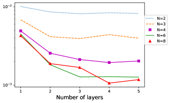
Figure 2: Test errors against the depth of the two sub-networks $\Phi_{\rm PNN}$ and $\Phi_{\rm SNN}$ for PSNN for different output dimensions $N$. Here the $x$-axis is the value of $L_{1},L_{2}$ (with $L_{1}=L_{2}$). The $y$-axis gives the test error in $log$ scale. And curves in different colors depict the test error corresponding to different values of $N$.

We next test the convergence with respect to PSNN structures while fixing the dimension $N$. From the previous numerical tests, it is sufficient to take $N=8$. Figure 3 summarizes our convergence tests for the network $\Phi_{\rm PNN}$ and $\Phi_{\rm SNN}$ separately. In Figure 3(A), we plot the error against depth of $\Phi_{\rm SNN}$ for several values of the width of $\Phi_{\rm SNN},$ while the structure of $\Phi_{\rm PNN}$ is fixed with $4$ layers and $60$ neurons in each layer. In contrast, Figure 3(B) shows the test error against the depth for varied number of width of $\Phi_{\rm PNN}$, while the structure of $\Phi_{\rm SNN}$ is fixed with $3$ layers and $20$ neurons in each layer. By comparing the different curves in Figure 3, one can observe the decrease in test erro as the sizes of $\Phi_{\rm PNN}$ and $\Phi_{\rm SNN}$ increase. Additionally, it is worth noticing that the error decreases much faster with respect to the size increase for the solution-network than the parameter-network. This observation is consistent with our analysis presented in Section 3 based on the different regularity of the target function $\Phi(U,\Theta)$ in its variables $\Theta$ and $U$.

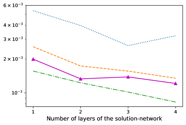
(a)

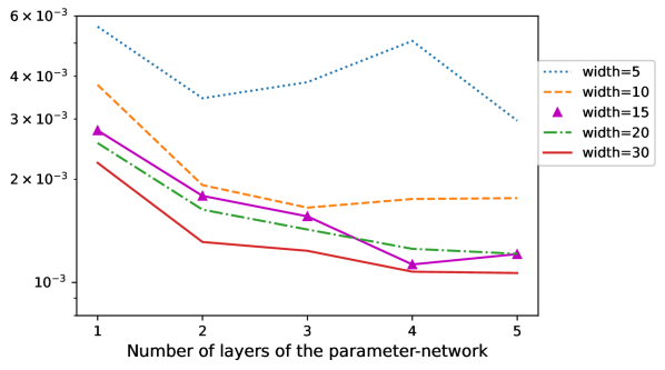
(b)

Figure 3: Test errors against the depth with varying width for the PSNN with a fixed dimension $N=8$ of the output vectors from the two sub-networks. The $x$-axis represents the value of $L_{1}$ (or $L_{2}$), and the $y$-axis gives the test error in $log$ scale. (a) $\Phi_{\rm SNN}$ is tested for $L_{2}=1,2,3,4$ and $W_{2}=5,10,15,20,$ and $\Phi_{\rm PNN}$ has the fixed structure: $L_{1}=4,W_{1}=30.$ (b) $\Phi_{\rm PNN}$ is tested for $L_{2}=1,2,3,4,5$ and $W_{2}=5,10,15,20,30,$ and $\Phi_{\rm SNN}$ has the fixed structure: $L_{1}=3,W_{1}=20.$

4.3 Locating solutions and phase boundaries

We now present numerical results to show how our trained PSNN and the post-processing algorithm, Algorithm 3, can help determine the number of multiple solutions, locate such solutions approximately, and predict the stability of such solutions. We also show the error between the predicted solutions and the exact solutions. The prediction of the number of solutions and their stability properties corresponding to the given parameters is described by phase diagrams, which consist of phase boundaries in the parameter space $\Omega$. For the Gray–Scott model, the exact parameter phase boundary for solution and the parameter phase boundary for stability are given explicitly in (23) and (24), respectively.

We take the training data set and the test data set same as those described in Section 4.2. The dimensions of the parameter network are set to $L_{1}=4$ and $W_{1}=30$, while the dimensions of the solution network are $L_{2}=3$ and $W_{2}=20$. The dimension $N$ of the output vectors from these sub-networks is set to be $N=8.$ The maximum allowable number of solutions, denoted as $C_{\rm max}$, is fixed at 5; that is, the algorithms will check the range from 0 to 5 and then determine the number of solutions each parameter pair is associated with.

The phase diagrams and the average error of locating solutions of two given algorithms are presented as follows. We compare the PSNN-based algorithm (see Algorithm 3) and the naive mean-shift-based algorithm (see Algorithm 4) using the same fixed training and test data sets. The phase diagrams for solution prediction for different parameters are plotted in Figure 4. Different colors in these plots correspond to different numbers of predicted solutions. It is noticeable that the PSNN-based algorithm generally provides accurate predictions for the number of solutions corresponding to each parameter (see Figure 4(A)). Therefore, the phase boundary can be predicted quite faithfully using the algorithm. The mean-shift-based algorithm (see Figure 4(B)), however, does a poor job of predicting the number of solutions, especially when the number of solutions is non-zero.

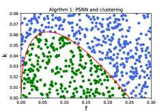
(a) PSNN-based algorithm

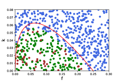
(b) Mean-shift-based algorithm

Figure 4: The phase diagram for solution prediction. The algorithms are set up to forecast the number of solutions within range $\{0,1,,\dots,5\}.$ The blue points represent the parameter pairs that the algorithm recognized as no-solution, and the brown points, green points and orange points respectively correspond to 1-solution, 2-solution, 3-and-more-solution. The red curve represents the phase boundary of $\Omega_{0}$ and $\Omega_{1}$, which is given by the formula $f-4(f+k)^{2}=0$.

In addition, we use $\Phi^{s}_{\text{PSNN}}$ to predict the stability of the learned solutions and the corresponding phase diagram is shown in Figure 5. An additional phase boundary curve is added that distinguishes stable solutions from unstable solutions in the region $\Omega_{2}$. One can observe that the predicted result shows high consistency with the true phase boundaries.

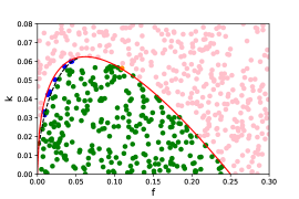
Figure 5: The Phase diagram for solution prediction with stability information. The algorithm is set to forecast the stability of learned solutions. The blue points, green points, brown points respectively represent 2-unstable-solution, 1-stable-1-unstable-solution, 2-stable-solution, and the black dashed curve plotted on $f\sqrt{f^{2}-4f(f+k)^{2}}+f^{2}-2(f+k)^{3}=0$ gives the boundary of $\Omega_{1,1}$ and $\Omega_{1,2}$.

4.4 Incomplete data

In practical applications, observation data may not be complete, as defined in Section 2.4. Here, we perform numerical tests on training our neural networks with incomplete data sets to examine if our approach and algorithms can be generalized. In this subsection, we take a training data set $\mathcal{T}_{\rm train}$ with $|I_{\rm train}|=1200$ and $N_{\rm random}=200$ and the test data set is the same as described in Section 4.2. Among the parameters for which two solutions exist (approximately 510 out of the 1200 parameters), we take 120 of them and remove one of the two solutions for each in the observation data set to form an incomplete observation data set. Furthermore, we perform a concentrated sampling technique designed to be compatible with incomplete data sets. For a complete data set, one can select $N_{\rm random}$ sampled points within the vicinity of each observed solution. This is illustrated by the left picture in Figure 6, where $200$ random points are sampled from two neighborhoods of radius $2\delta(\Theta)$ of the observed solutions for a given parameter $\Theta=(f,k)$. Note that $\delta(\Theta)$ is defined in (6). With an incomplete data set, the information surrounding the missing solution is removed, and we only sample points from the vicinity of the remaining observed solutions. The right picture in Figure 6 illustrates that when only one solution is observed for the same parameter $\Theta=(f,k)$, we only sample $100$ random points from a neighborhood of radius $2\tilde{\delta}(\Theta)$ of the observed solution. The determination of $\tilde{\delta}(\Theta)$ is carried out as follows. For a given parameter $\Theta$, let $n(\Theta)$ denote the number of observed solutions in a given (incomplete) data set. Define $m_{\epsilon}(\Theta):=\max\{n(\bar{\Theta}):\bar{\Theta}\in\mathcal{N}_{\epsilon}(\Theta)\}$, where $\mathcal{N}_{\epsilon}(\Theta)\subset\Omega$ denotes a neighborhood of $\Theta$ dictated by a small number $\epsilon>0$. Then we define

(25) $$\tilde{\delta}(\Theta)=\text{mean}\{\delta(\bar{\Theta}):\delta(\bar{\Theta})=m_{\epsilon}(\Theta)\text{ for }\bar{\Theta}\in\mathcal{N}_{\epsilon}(\Theta)\}.$$

Note that in the above definition, for any $\bar{\Theta}\in\mathcal{N}_{\epsilon}(\Theta)$, $\delta(\bar{\Theta})$ is computed by the formula in (6) where $S^{\bar{\Theta}}$ is taken as the observed (incomplete) solution set. The objective is to have $\tilde{\delta}(\Theta)$ serve as an approximation to the true value $\delta(\Theta)$ computed with a complete observation of solutions. In our experiment, we take $\mathcal{N}_{\epsilon}(\Theta)$ to be a neighborhood of $\Theta$ that contains a few numbers of other parameters to ensure a large likelihood that $\tilde{\delta}(\Theta)$ approximates the true value.

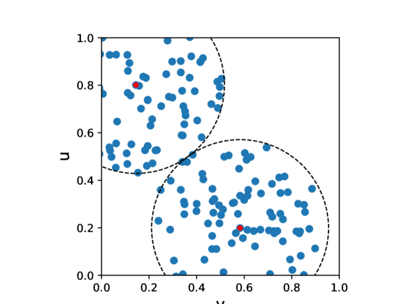
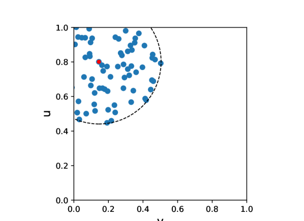
Figure 6: Comparison of complete data points (left) with incomplete data points (right) for a given pair $\Theta=(f,k)$ for which two solutions exist. Left: 200 randomly selected points in two neighborhoods of radius $2\delta(\Theta)$ of the observed solutions. Right: 100 randomly selected points with a neighborhood of $2\tilde{\delta}(\Theta)$ the observed solution. $\delta(\Theta)$ and $\tilde{\delta}(\Theta)$ are defined in Eqs. 6 and 25, respectively.

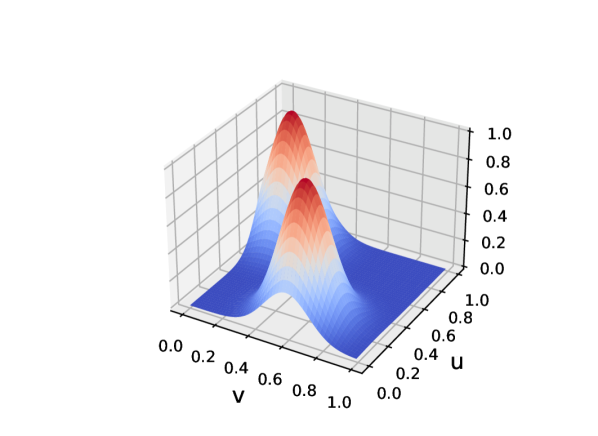
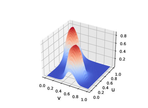
Figure 7: With the same parameter pair $\Theta=(f,k)$ in Figure 6, the left figure shows the target function $\Phi((u,v),(f,k))$, and the right figure shows the PSNN-recovered function $\Phi_{\text{PSNN}}((u,v),(f,k))$ with the incomplete complete training data. PSNN recovers the missing information surrounding one of the solutions.

We observe that the trained PSNN on incomplete data successfully covers the missing information, as illustrated by Figure 7. The left plot in Figure 7 shows the target function $\Phi$ for the same parameter $\Theta$ chosen in Figure 6. In particular, the training data set has no information around the missing solution corresponding to the given parameter (cf. Figure 6(right)). Yet, as shown by the right plot in Figure 7, the trained PSNN successfully predicted the function surrounding the missing solution.

Additionally, we use the trained PSNN on incomplete data for solution prediction and draw the phase diagram in Figure 8 in comparison with the one predicted by the mean-shift-based algorithm. With incomplete data, the PSNN-based algorithm again successfully predicts the phase diagram, similar to the one in Figure 4. In Table 1, quantitative errors for solution prediction on both complete and incomplete data sets are presented. For the experiment with incomplete data, in addition to the test on the randomly chosen test data set, we also record the algorithm prediction for the $120$ parameters with missing information in the observation data. PSNN demonstrates effectiveness cross all tests. As a comparison, the naive mean-shift-based algorithm exhibits significantly poorer performance than the PSNN-based algorithm, particularly on the lost data set.

Training set	Test set	PSNN			Mean-shift
		Wrong-soln	Distance	Wrong-stb	Wrong-soln	Distance
Complete	Random	1.22%	0.020	5.12%	14.06%	0.149
Incomplete	Random	1.22%	0.020	4.58%	14.22%	0.149
	Lost data	0.56%	0.018	0%	36.94%	0.147

Table 1: Error table of PSNN-based algorithm and mean-shift-based algorithm using the complete/incomplete data, and performed on random/lost test data. Wrong-soln counts the percentage of parameters for which the algorithm fails to determine the correct number of solutions. Distance signifies the average relative distance (as defined in (13)) between the predicted solution set and the exact solution set of the parameters where the number of solutions has been correctly predicted. And Wrong-stb denotes the percentage of parameters for which the algorithm’s predictions on stability were inaccurate. To reduce the impact of randomness, we performed each set of experiments three times and evaluated the two algorithms on three separate test sets, calculating the average results.

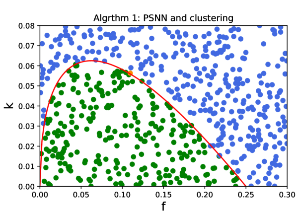
(a) PSNN-based algorithm with incomplete data

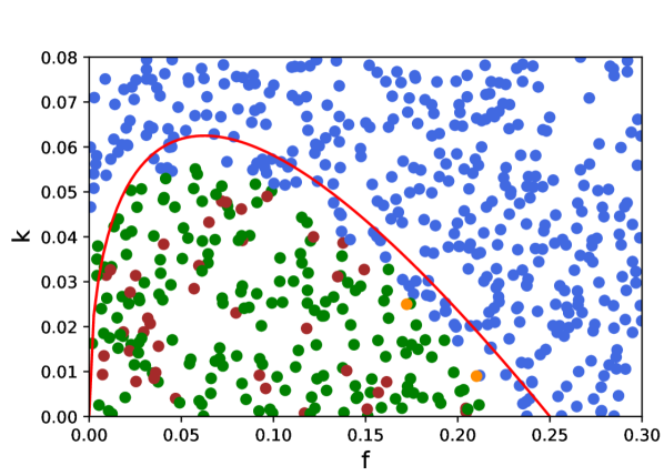
(b) Mean-shift-based algorithm with incomplete data

Figure 8: Phase diagrams for solution prediction using incomplete data. Similar to Fig. 4, the blue points, the brown points, green points and orange points respectively represent the parameter pairs that the algorithm recognized as no-solution 1-solution, 2-solution, 3-and-more-solution, and the red curve represents the phase boundary of $\Omega_{0}$ and $\Omega_{1}$.

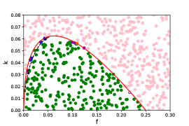
Figure 9: The hase diagram for solution prediction with stability information using incomplete data. The blue points, green points, brown points respectively represent 2-unstable-solution, 1-stable-1-unstable-solution, 2-stable-solution, and the black dashed curve plotted on $f\sqrt{f^{2}-4f(f+k)^{2}}+f^{2}-2(f+k)^{3}=0$ gives the boundary of $\Omega_{1,1}$ and $\Omega_{1,2}$.

Finally, we train $\Phi^{s}_{\rm PSNN}$ on the incomplete data set, and the phase diagram for stability is presented in Figure 9. The above studies show that even trained with incomplete data, the PSNN-based algorithm continues to excel in forecasting the number of solutions for given parameters, predicting the phase boundary in parameter space, and determining the stability of learned solutions.

5 Conclusion

Systems of ordinary differential equations (ODEs) and dynamical systems with many parameters are widely used in scientific modeling with emerging applications. Identifying parameters for which solutions of such systems exist and possess distinguished properties is a challenging task, particularly for complex and large systems with many parameters. Here, we have initiated the development of a machine learning approach to tackle such an important and difficult problem.

We have first introduced target functions, $\Phi=\Phi(U,\Theta)$ and $\Phi^{\rm s}(U,\Theta),$ that characterize the desired parameter-solution properties, and then constructed parameter-solution neural networks (PSNNs), $\Phi_{\rm PSNN}$ and $\Phi^{\rm s}_{\rm PSNN}$, for studying solutions and the stability of solutions, respectively. Each of these neural networks couples a parameter-network and a solution-network with different structures, allowing us to treat the parameters and solutions differently due to the different regularities of the target functions for different variables. We have also developed numerical methods to locate solutions and determine their stability with our trained networks. We have presented a detailed analysis to show the convergence of our designed neural networks to the target functions with respect to the increase in network sizes, and have also obtained the related error estimates. Our extensive numerical results on the Gray–Scott model have confirmed our rigorous convergence analysis and also have demonstrated that our approach can predict phase boundaries for solutions and the stability of solutions. In contrast to traditional techniques, our new approach, which is developed with the help of rigorous analysis, makes it possible to explore efficiently the entire solution space corresponding to each parameter, and further locate the multiple solutions approximately and determine their solution stability.

While our initial studies are promising, we would like to address several issues for the further development of our theory and numerical methods. First, we have used one target function $\Phi$ for solutions and another $\Phi^{s}$ for their stability. It may be desirable if these two can be combined to make the approach more efficient. Moreover, it demands further consideration and innovative approaches to manage large systems effectively. For example, our post-processing method for locating solutions for a given parameter $\Theta\in\Omega$ relies on a set of sample points $\mathcal{U}\subset D$ generated from uniform grids on $D$. For a high-dimensional problem, where the dimension of the solution vector is large, our method may not be feasible as the number of data points in $\mathcal{U}$ can be large. Alternative algorithms for locating solutions more efficiently for high-dimensional problems need to be designed. A key question is the selection of a density from which to sample the points. Lastly, training networks with incomplete data is crucial in applications, especially for large systems. Missing information in incomplete data, however, may be recovered from the structure of the underlying systems, as demonstrated by our initial examples in Section 4.4. Additionally, methods of unsupervised learning may be considered in the future to train networks with incomplete data. Last but not least, applications of our framework to more realistic parameterized dynamic systems and/or parameterized nonlinear systems of algebraic equations will be considered in the future.

Appendix A Mean-shift algorithm

Input: A parameter $\Theta\in\Omega$, a training set $\mathcal{T}_{\rm train}$ (cf. (11)), a cut value $L_{\rm cut}\in(0,1),$, two numerical parameters $\gamma_{\rm P}>0$ and $\gamma_{\rm S}>0$ for defining neighbords in $\Omega$ and $D$, respectively, and a tolerance $\epsilon_{\rm tol}$.

Output: The set of centers $\mathcal{U}^{\Theta}\subset S^{\Theta}$

let $y_{j}^{i}=\Phi(U_{j}^{i},\Theta_{i})$ for $j=1,\cdots,S+\mathcal{N}_{m_{i}}$, and $i=1,2,\cdots,P$ ;

define neighbor($\tilde{U},\tilde{\Theta}$):= $\{(U_{j}^{i},\Theta_{i}):\|\Theta_{i}-\tilde{\Theta}\|_{l^{\infty}}<\gamma_{\rm P},\|U^{i}_{j}-\tilde{U}\|_{l^{\infty}}<\gamma_{\rm S}\}$;

Function Meanshift($\Theta,\gamma_{\rm P},\gamma_{\rm S},\epsilon_{\rm tol}$)

       Pick $U\in D$ randomly;

       $\epsilon\leftarrow 1$;

       condition $\leftarrow$ True;

       while $\epsilon\geq\epsilon_{\rm tol}$ and condition= True do

             if $y_{\text{sum}}:=\underset{\textnormal{{neighbor(}}\textnormal{\emph{$U,\Theta$}}\textnormal{{)}}}{\sum}y^{i}_{j}>0$ then

                   $U^{0}\leftarrow U$ ;

                   $U\leftarrow\underset{\textnormal{{neighbor(}}\textnormal{\emph{$U,\Theta$}}\textnormal{{)}}}{\sum}\frac{y^{i}_{j}}{y_{\text{sum}}}U_{j}^{i}$;

                   $\epsilon\leftarrow$ dist($U,U^{0}$)

            else

                   condition $\leftarrow$ False

            

      if condition then

             return $U$

      

select $\epsilon_{\rm tol}\in(0,1)$;

set $\mathcal{U}_{\rm collected}$ to be an empty set;

for $1\leq k\leq N_{initial}$ do

       $U_{M}\leftarrow$ Meanshift($\Theta,\gamma_{\rm P},\gamma_{\rm S},\epsilon_{\rm step}$)

      if $\frac{1}{|\textnormal{{neighbor(}}\textnormal{\emph{$U_{M},\Theta$}}\textnormal{{)}}|}\underset{\textnormal{{neighbor(}}\textnormal{\emph{$U_{M},\Theta$}}\textnormal{{)}}}{\sum}y^{i}_{j}\geq L_{\rm cut}$ then

             Collect $U_{M}$ to $\mathcal{U}_{\rm collected}$

      

obtain $\mathcal{U}_{c}\leftarrow$ Cluster($\mathcal{U}_{\rm collected}$) where Cluster is given in Algorithm 3;

Algorithm 4 Finding solutions by mean-shift and clustering

References

• [1] R. A. Adams and J. J. Fournier, Sobolev spaces, Elsevier, 2003.
• [2] E. L. Allgower and K. Georg, Numerical Continuation Methods: An Introduction, vol. 13, Springer Science & Business Media, 2012.
• [3] D. Comaniciu and P. Meer, Mean shift analysis and applications, in Proceedings of the Seventh IEEE International Conference on Computer Vision, vol. 2, 1999, pp. 1197–1203 vol.2.
• [4] J. B. Conway, A Course in Functional Analysis, Springer–Verlag, 2nd ed., 1990.
• [5] P. Deuflhard, Newton Methods for Nonlinear Problems: Affine Invariance and Adaptive Algorithms, vol. 35, Springer Science & Business Media, 2005.
• [6] P. E. Farrell, A. Birkisson, and S. W. Funke, Deflation techniques for finding distinct solutions of nonlinear partial differential equations, SIAM Journal on Scientific Computing, 37 (2015), pp. A2026–A2045.
• [7] A. Gierer and H. Meinhardt, A theory of biological pattern formation, Kybernetik, 12 (1972), pp. 30–39.
• [8] P. Gray and S. K. Scott, Autocatalytic reactions in the isothermal, continuous stirred tank reactor, Chemical Engineering Science, 18 (1983), pp. 29–43.
• [9] P. Gray and S. K. Scott, Autocatalytic reactions in the isothermal, continuous stirred tank reactor, Chemical Enginnering Science, 39 (1984), pp. 1087–1097.
• [10] P. Gray and S. K. Scott, Sustained oscillations and other exotic patterns of behavior in isothermal reactions, Journal of Physical Chemistry, 89 (1985), pp. 22–32.
• [11] W. Hao and C. Zheng, Learn bifurcations of nonlinear parametric systems via equation-driven neural networks, Chaos: An Interdisciplinary Journal of Nonlinear Science, 32 (2022).
• [12] A. Hastings, Population Biology: Concepts and Models, Springer, 1996.
• [13] M. W. Hirsch, S. Smale, and R. L. Devaney, Differential Equations, Dynamical Systems, and an Introduction to Chaos, Academic Press, 3rd ed., 2012.
• [14] M. A. Hjortso and P. R. Wolenski, Linear Mathematical Models In Chemical Engineering, World Scientific, 2010.
• [15] Y. Huang, W. Hao, and G. Lin, HomPINNs: Homotopy physics-informed neural networks for learning multiple solutions of nonlinear elliptic differential equations, Computers & Mathematics with Applications, 121 (2022), pp. 62–73.
• [16] D. P. Kingma and J. Ba, ADAM: A method for stochastic optimization, arXiv preprint arXiv:1412.6980, (2014).
• [17] W.-C. Lo, L. Chen, M. Wang, and Q. Nie, A robust and efficient method for steady state patterns in reaction–diffusion systems, Journal of Computational Physics, 231 (2012), pp. 5062–5077.
• [18] J. Mercer, Functions of positive and negative type, and their connection the theory of integral equations, Philosophical Transactions of the Royal Society of London. Series A, 209 (1909), pp. 415–446.
• [19] H. Q. Minh, P. Niyogi, and Y. Yao, Mercer’s theorem, feature maps, and smoothing, in Learning Theory, G. Lugosi and H. U. Simon, eds., Berlin, Heidelberg, 2006, Springer Berlin Heidelberg, pp. 154–168.
• [20] J. E. Pearson, Complex patterns in a simple system, Science, 261 (1993), pp. 189–192.
• [21] L. Perko, Differential Equations and Dynamical Systems, Springer, 3rd ed., 2001.
• [22] P. Petersen and F. Voigtlaender, Optimal approximation of piecewise smooth functions using deep ReLU neural networks, Neural Networks, 108 (2018), pp. 296–330.
• [23] F. Pichi, Reduced Order Models for Parametric Bifurcation Problems in Nonlinear PDEs, PhD thesis, SISSA, 2020.
• [24] F. Pichi, F. Ballarin, G. Rozza, and J. S. Hesthaven, An artificial neural network approach to bifurcating phenomena in computational fluid dynamics, Computers & Fluids, 254 (2023), p. 105813.
• [25] A. Polynikis, S. J. Hogan, and M. di Bernardo, Comparing different ODE modelling approaches for gene regulatory networks, Journal of Theoretical Biology, 261 (2009), pp. 511–530.
• [26] C. Schwab and R. A. Todor, Karhunen–Loève approximation of random fields by generalized fast multipole methods, Journal of Computational Physics, 217 (2006), pp. 100–122.
• [27] K. P. Sinaga and M.-S. Yang, Unsupervised k-means clustering algorithm, IEEE Access, 8 (2020), pp. 80716–80727.
• [28] S. H. Strogatz, Nonlinear Dynamics and Chaos, CRC Press, 2nd ed., 2015.
• [29] P. Turchin, Complex Population Dynamics: A Theoretical/Empirical Synthesis, vol. 35 of Monographs in Population Biology, Princeton University Press, 2003.
• [30] A. M. Turing, The chemical basis of morphogenesis, Philosophical Transactions of the Royal Society B, 237 (1952), pp. 37–72.
• [31] D. Walgraef, Spatio-Temporal Pattern Formation, Springer, 1997.
• [32] J. Xu, A novel two-grid method for semilinear elliptic equations, SIAM Journal on Scientific Computing, 15 (1994), pp. 231–237.
• [33] D. Yarotsky, Error bounds for approximations with deep ReLU networks, Neural Networks, 94 (2017), pp. 103–114.
• [34] J. Yin, Y. Wang, J. Z. Chen, P. Zhang, and L. Zhang, Construction of a pathway map on a complicated energy landscape, Physical Review Letters, 124 (2020), p. 090601.
• [35] H. Zheng, Y. Huang, Z. Huang, W. Hao, and G. Lin, HomPINNs: Homotopy physics-informed neural networks for solving the inverse problems of nonlinear differential equations with multiple solutions, arXiv preprint arXiv:2304.02811, (2023).
• [36] J. Zhou, Solving multiple solution problems: Computational methods and theory revisited, Communication on Applied Mathematics and Computation, 31 (2017), pp. 1–31.