Symmetry breaking of $3$-dimensional AdS in holographic semiclassical gravity

Akihiro Ishibashi¹, Kengo Maeda² and Takashi Okamura³

¹Department of Physics and Research Institute for Science and Technology,

Kindai University, Higashi-Osaka, Osaka 577-8502, JAPAN

²Faculty of Engineering, Shibaura Institute of Technology,

Saitama 330-8570, JAPAN

³Department of Physics and Astronomy, Kwansei Gakuin University,

Sanda, Hyogo, 669-1330, JAPAN

akihiro at phys.kindai.ac.jp, maeda302 at sic.shibaura-it.ac.jp
tokamura at kwansei.ac.jp

1 Introduction

One of the important issues in quantum general relativity is whether spacetime is stable under quantum effects. One approach to addressing such a problem is the semiclassical approximation in which gravitational field is treated classically, while matter fields quantum mechanically: Classical gravity obeys the semiclassical Einstein equations sourced by the vacuum expectation value of the renormalized stress-energy tensor for quantum matter fields. In this approach, Minkowski spacetime, for example, was found to be unstable against a certain type of quantum fluctuations [1, 2, 3]. However, it is in general difficult to analyze such semiclassical problems for curved spacetimes, except for a few special cases (see e.g., [4, 5]).

Recently, the semiclassical Einstein equations have been reformulated in the holographic context [6, 7], in which $d$-dimensional metric on the conformal boundary of $(d+1)$-dimensional anti-de Sitter (AdS_d+1) bulk spacetime is promoted to be a dynamical field induced by boundary quantum conformal field theory (CFT). In this formulation, the $d$-dimensional semiclassical Einstein equations can be viewed as a mixed boundary conditions for the $(d+1)$-dimensional bulk classical metric, and the vacuum expectation value for quantum matter fields—whose evaluation is one of the hardest parts of the job in semiclassical problems—can be explicitly computed by exploiting the well-known formulas [11] of the AdS/CFT correspondence [8, 9, 10]. In this way, the holographic approach considerably simplifies the problem of how to set up the semiclassical Einstein equations, especially how to compute the source term, and at the same time makes it possible to analyze the effects of strongly coupled quantum fields on the dynamics of classical gravity.

In our previous paper [7], by taking advantage of the holographic approach mentioned above, we have analyzed the semiclassical Einstein equations and shown that the covering space of $3$-dimensional static BTZ black hole is semiclassically unstable under linear perturbations due to strongly coupled CFTs. We have introduced the universal parameter $\gamma_{3}$ which determines the onset of semiclassical instabilities. We have also shown the existence of a $3$-dimensional static asymptotically AdS semiclassical solution with a non-zero expectation value for stress-energy tensor, which may be interpreted as an asymptotically AdS black hole with “quantum hair.”

In this paper, we further study the issue of holographic semiclassical instability of AdS₃ from the thermodynamic viewpoint. For this purpose, we investigate perturbations of semiclassical AdS₃ with vanishing expectation value of the stress-energy tensor and evaluate free energy by calculating the on-shell action at second order in perturbation. We find that the only non-zero terms in our action for the holographic setting with AdS₄ bulk and AdS₃ boundary are the $2$-dimensional surface terms of semiclassical AdS₃ solution. By adding appropriate counter term with respect to the $2$-dimensional surface, we find that the free energy for the semiclassical solution with non-vanishing stress energy tensor is always smaller than that of the background AdS₃ solution with vanishing expectation values for the stress-energy tensor. For comparison with our previous work [7], we perform the analysis in both the covering space of static BTZ black hole (i.e., AdS₃ background with Killing horizon) as well as the global AdS₃ (i.e., the manifestly zero-temperature background with no horizon). For both cases, we arrive at the same conclusion that AdS₃ as a solution to the semiclassical Einstein equations with vanishing source term can be thermodynamically unstable, of which onset is determined by the control parameter $\gamma_{3}$ introduced in [7]. In particular, it is clear from the analysis of the global AdS₃ case that the quantum field on our AdS₃ is in the conformal vacuum state. This instability implies that the maximal symmetries of AdS₃ break down spontaneously, suggesting that a phase transition occurs between the semiclassical AdS₃ solution with vanishing stress-energy tensor and that with non-vanishing stress-energy tensor. This is a new instability, different from the well-known semiclassical linear instaiblity [1, 2, 3, 13, 14] since our holographic semiclassical Einstein equations do not involve higher order derivative terms.

This paper is organized as follows. In section 2, we will provide a general prescription for deriving the second variation of the on-shell action. In section 3, we give analytic semiclassical AdS solutions with non-zero expectation values of the stress-energy tensor within perturbation. In section 4, we evaluate the free energy of the analytic solutions based on the prescription in section 2. Section 5 is devoted to summary and discussions. The notation and conventions essentially follow our previous work [7].

2 The second variation of the on-shell action

In this section, we evaluate the second-order variation of the effective action by using the AdS/CFT correspondence. We consider a $4$-dimensional AdS bulk spacetime with the metric

$$ds_{4}^{2} =G_{MN}(X)dX^{M}dX^{N}$$

$$=\Omega^{-2}(z)dz^{2}+g_{\mu\nu}(z,x)dx^{\mu}dx^{\nu}$$

$$=\Omega^{-2}(z)(dz^{2}+\tilde{g}_{\mu\nu}(z,x)dx^{\mu}dx^{\nu})\,,$$ (2.1)

where $X^{M}=(z,x^{\mu})$ and $\Omega$ is a conformal factor which vanishes on the AdS conformal boundary at $z=0$. The conformal boundary metric $\mathcal{G}_{\mu\nu}$ is defined by

$$\mathcal{G}_{\mu\nu}(x):=\lim_{z\to 0}\Omega^{2}(z)G_{\mu\nu}(z,\,x)=\lim_{z\to 0}\tilde{g}_{\mu\nu}(z,\,x)\,.$$ (2.2)

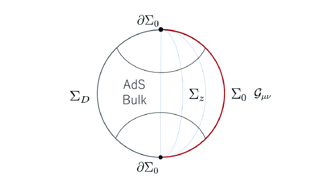
Figure 1: A time-slice of the (conformally compactified) AdS bulk spacetime foliated by $z=const$. hypersurfaces $\Sigma_{z}$ (denoted by the dotted curve), each of which itself is an asymptotically AdS spacetime one dimensional lower than the bulk AdS. The conformal boundary of the bulk AdS is divided into the left-part $\Sigma_{D}$ and the right-part $\Sigma_{0}$, and these two are matched at the corner $\partial\Sigma_{0}$. On the-right part $\Sigma_{0}$, the boundary metric is supposed to satisfy the holographic semiclassical Einstein equations, or in other words the mixed boundary condition is imposed on the bulk metric. For definiteness we assume that on the left-part $\Sigma_{D}$, the Dirichlet boundary conditions are imposed on the bulk metric. When $\Sigma_{0}$ includes a $3$-dimensional boundary black hole, the bulk spacetime also includes a $4$-dimensional black hole with a horizon $H$ inside the bulk. The two hyperbolic curves denote one of the possible bulk horizons.

We assume that each $z=const.$ hypersurface—denoted by $\Sigma_{z}$—with the metric $\tilde{g}_{\mu\nu}(z,x)$ is asymptotically AdS₃ and that the AdS₄ bulk spacetime is foliated by a family of $\Sigma_{z}$, as shown in Fig. 1. Then, the limit hypersurface $\Sigma_{0}:=\lim_{z\to 0}\Sigma_{z}$ is a portion of the conformal boundary $\partial M$. We are concerned with the dynamics of $\Sigma_{0}$ which, in our setup, satisfies the holographic semiclassical Einstein equations. Following [7], we shall impose the Dirichlet boundary condition at the other part of the conformal boundary $\Sigma_{D}:=\partial M\setminus\{\Sigma_{0}\cup\partial\Sigma_{0}\}$ (see Fig. 1). The semiclassical Einstein equations are represented as a mixed boundary condition at $\Sigma_{0}$ for the bulk metric $G_{MN}$. Depending on the geometry of $\Sigma_{0}$, (e.g., when $\Sigma_{0}$ includes a $3$-dimensional black hole), the bulk spacetime may admit an inner boundary $H$ (e.g., the horizon of a $4$-dimensional bulk black hole or black string). See Fig. 1.

The total effective action ${\mathcal{S}}$ for a $3$-dimensional semiclassical problem is constructed by the $3$-dimensional Einstein-Hilbert action ${\mathcal{S}}_{\text{EH}}$, the $2$-dimensional Gibbons-Hawking term ${\mathcal{S}}_{\text{GH}}$, the $2$-dimensional counter term ${\mathcal{S}}_{\text{ct}}$, and the effective action $\Gamma$ for $3$-dimensional CFT as

$${\mathcal{S}}={\cal S}_{\text{EH}}+{\mathcal{S}}_{\text{GH}}+{\mathcal{S}}_{\text{ct}}+\Gamma\,,$$ (2.3)

where

$${\mathcal{S}}_{\text{EH}}=\frac{1}{16\pi G_{3}}\int_{\Sigma_{0}}d^{3}x\sqrt{-\mathcal{G}}\left(\mathcal{R}-2\Lambda_{3}\right)\,,$$ (2.4)

with $G_{3}$, $\mathcal{R}$, and $\Lambda_{3}$ being, respectively, the $3$-dimensional gravitational constant, the scalar curvature, and the cosmological constant on $(\Sigma_{0},\mathcal{G}_{\mu\nu})$, and where $\Gamma$ gives ries to the expectation value of stress-energy tensor for CFT:

$$\left\langle~{}\mathcal{T}_{\mu\nu}~{}\right\rangle=-\dfrac{2}{\sqrt{-\mathcal{G}}}\,\dfrac{\delta\Gamma}{\delta\mathcal{G}^{\mu\nu}}\,.$$ (2.5)

According to the AdS/CFT correspondence, the effective action $\Gamma$ for CFT in (2.3) is given in terms of the bulk gravity dual. More precisely, $\Gamma$ is identified with the on-shell value of the bulk action $S_{\text{bulk}}$, composed of the $4$-dimensional Einstein-Hilbert action $S_{\text{EH}}$, the $3$-dimensional Gibbons-Hawking term $S_{\text{GH}}$, and the counter term $S_{\text{ct}}$, as

$$S_{\text{bulk}}=S_{\text{EH}}+S_{\text{GH}}+S_{\text{ct}},$$

$$S_{\text{EH}}=\frac{1}{16\pi G_{4}}\int d^{4}X\sqrt{-G}\left(R(G)+\frac{6}{L^{2}}\right),$$

$$S_{\text{GH}}=\frac{1}{8\pi G_{4}}\int d^{3}x\sqrt{-g}\,K,$$

$$S_{\text{ct}}=-\frac{1}{16\pi G_{4}}\int d^{3}x\sqrt{-g}\left(\frac{4}{L}+LR(g)\right)\,,$$ (2.6)

where $G_{4}$ and $L$ denote the $4$-dimensional gravitational constant and the curvature length, respectively, and where $R(G)$, $R(g)$ the scalar curvature of the bulk metric $G_{MN}$ and that of the induced metric $g_{\mu\nu}$ on $\Sigma_{z}$, respectively. Here, the extrinsic curvature $K_{\mu\nu}$ is defined by

$$K_{\mu\nu}=-\frac{\Omega}{2}\partial_{z}g_{\mu\nu}\,.$$ (2.7)

Since our effective action (2.3) includes the Einstein-Hilbert term (2.4) on the conformal boundary $\Sigma_{0}$, the conformal boundary metric $\mathcal{G}_{\mu\nu}$ becomes dynamical [6]. Therefore, by varying the bulk metric $G_{MN}$ and $\mathcal{G}_{\mu\nu}$ independently, we can obtain both the bulk Einstein equations and the boundary semiclassical Einstein equations:

$$R_{MN}-\frac{1}{2}R\,G_{MN}-\frac{3}{L^{2}}G_{MN}=0,$$

$${\mathcal{R}}_{\mu\nu}-\frac{\mathcal{R}}{2}\mathcal{G}_{\mu\nu}-\frac{1}{\ell^{2}}\mathcal{G}_{\mu\nu}-8\pi G_{3}\langle~{}\mathcal{T}_{\mu\nu}~{}\rangle=0\,,$$ (2.8)

where $\ell$ is the curvature length $\ell^{2}=-1/\Lambda_{3}$ and $\langle~{}\mathcal{T}_{\mu\nu}~{}\rangle$ is given by (2.5).

As shown in [7], the solution is obtained perturbatively by expanding the conformal (unphysical) metric $\tilde{g}_{\mu\nu}(z,\,x)$ as

$$\tilde{g}_{\mu\nu}(z,\,x)={\bar{g}}_{\mu\nu}(x)+\epsilon h_{\mu\nu}(z,\,x)+O(\epsilon^{2})\,,$$ (2.9)

where $\epsilon$ is an infinitesimally small parameter and ${\bar{g}}_{\mu\nu}(x)=\bar{\mathcal{G}}_{\mu\nu}(x)$ is the background boundary metric:

$$d\bar{s}_{3}^{2}=-\frac{f}{u}dt^{2}+\frac{\ell^{2}}{4u^{2}f}du^{2}+\frac{\ell^{2}d\varphi^{2}}{u},\qquad f:=1-8\pi G_{3}{\cal M}\,u$$ (2.10)

with some constant $\cal M$, satisfying

$$\bar{\mathcal{R}}_{\mu\nu}=-\frac{2}{\ell^{2}}\bar{\mathcal{G}}_{\mu\nu}\,.$$ (2.11)

Here, the case ${\cal M}>0$ corresponds to the BTZ metric if $\varphi$ is $2\pi$-periodic, while $8\pi G_{3}{\cal M}=-1$ to the global AdS₃ metric. Note that the case ${\cal M}=0$ corresponds to (a locally) AdS₃ in the Poincare chart and case ${\cal M}<0$ (but $8\pi G_{3}{\cal M}\neq-1$) to (a locally) AdS₃ with a conical singularity (if $\varphi$ is $2\pi$-periodically identified), and in what follows, we do not consider these two cases.

By using eqs. (2) and (2.11), the conformal factor $\Omega$ is determined by

$$\Omega(z)=\frac{\ell}{L}\sin\frac{z}{\ell}\,,$$ (2.12)

where $\Sigma_{0}$ and $\Sigma_{D}$ in Fig. 1 are located at $z=0$ and $z=\pi\ell$, respectively. Note that in the unperturbed case, $\epsilon=0$, the expectation value of the stress-energy tensor $\langle~{}\mathcal{T}_{\mu\nu}~{}\rangle$ vanishes, and therefore the semiclassical equations in eqs. (2) are trivially satisfied.

Now we holographically evaluate the second order variation of the effective action $\Gamma$ in (2.3) by inspecting the action for the gravity dual (2). Let us first examine the bulk Einstein-Hilbert action,

$$S_{\text{EH}}=\frac{1}{16\pi G_{4}}\int d^{4}X\left[\sqrt{-\tilde{g}}\left(\frac{{R}(\tilde{G})}{\Omega^{2}}-\frac{12\Omega^{\prime 2}}{\Omega^{4}}+\frac{6\Omega^{\prime\prime}}{\Omega^{3}}+\frac{6}{L^{2}\Omega^{4}}\right)+\frac{6\Omega^{\prime}}{\Omega^{3}}(\sqrt{-\tilde{g}})^{\prime}\right]\,,$$ (2.13)

where ${R}(\tilde{G})$ is the scalar curvature of the conformal metric $\tilde{G}_{MN}:=\Omega^{2}\,G_{MN}$ and the prime denotes the derivative with respect to $z$.

As our variation, we consider the tensor-type perturbations of the bulk metric which satisfy $h_{zz}=h_{z\nu}=0$, and

$${h_{\nu}}^{\nu}=h_{\mu\nu}\bar{g}^{\mu\nu}=0,\qquad\bar{D}^{\nu}h_{\nu\mu}=0\,,$$ (2.14)

where $\bar{D}_{\mu}$ is the covariant derivative with respect to the unperturbed boundary metric $\bar{g}_{\mu\nu}$.

By using eqs. (2.14) and (A), it is easily checked that the first variation of the bulk action (2.13) vanishes. With the help of the formulas (A) and (A), we obtain the second variation of the bulk action as

$$\delta^{2}S_{\text{EH}} =\frac{\epsilon^{2}}{16\pi G_{4}}\int d^{4}X\sqrt{-\bar{g}}\Biggl{[}\frac{3}{L^{2}\Omega^{4}}h_{\mu\nu}h^{\mu\nu}-\frac{3\Omega^{\prime}}{\Omega^{3}}(h_{\mu\nu}h^{\mu\nu})^{\prime}$$

$${}\quad+\frac{1}{\Omega^{2}}\Biggl{\{}-\frac{h_{\mu\nu}h^{\mu\nu}}{\ell^{2}}+\frac{1}{2}h^{\mu\nu}(\bar{D}^{2}h_{\mu\nu}+h_{\mu\nu}^{\prime\prime})+\frac{3}{4}(h_{\mu\nu}h^{\mu\nu})^{\prime\prime}+\bar{D}_{\mu}V^{\mu})\Biggr{\}}\Biggr{]}\,,$$ (2.15)

where $V^{\mu}$ is defined by

$$V^{\mu}:=\frac{3}{4}\bar{D}^{\mu}(h^{\alpha\beta}h_{\alpha\beta})-\bar{D}_{\nu}(h^{\mu\alpha}{h_{\alpha}}^{\nu})\,.$$ (2.16)

Using the following relations

$$\Omega^{\prime\prime}=-\frac{\Omega}{\ell^{2}}\,,\quad\frac{1-L^{2}\Omega^{\prime 2}}{L^{2}\Omega^{2}}=\frac{1}{\ell^{2}}\,,\quad h^{\prime}_{\mu\nu}h^{\mu\nu}=\frac{1}{2}(h_{\mu\nu}h^{\mu\nu})^{\prime}\,,$$ (2.17)

we can rewrite (2) as

$$\delta^{2}S_{\text{EH}} =\frac{\epsilon^{2}}{32\pi G_{4}}\int d^{4}X\frac{\sqrt{-\bar{g}}}{\Omega^{2}}h^{\mu\nu}\Biggl{\{}\Omega^{2}\left(\frac{h_{\mu\nu}^{\prime}}{\Omega^{2}}\right)^{\prime}+\left({\bar{D}}^{2}+\frac{2}{\ell^{2}}\right)h_{\mu\nu}\Biggr{\}}$$

$${}+\frac{\epsilon^{2}}{16\pi G_{4}}\int d^{4}X\sqrt{-\bar{g}}\biggl{[}\left\{\frac{3}{4\Omega^{2}}(h^{\mu\nu}h_{\mu\nu})^{\prime}-\frac{\Omega^{\prime}}{\Omega^{3}}h^{\mu\nu}h_{\mu\nu}\right\}^{\prime}+\frac{1}{\Omega^{2}}\bar{D}_{\mu}V^{\mu}\Biggr{]}$$

$$=\frac{\epsilon^{2}}{16\pi G_{4}}\int d^{4}X\sqrt{-\bar{g}}\biggl{[}\left\{\frac{3}{4\Omega^{2}}(h^{\mu\nu}h_{\mu\nu})^{\prime}-\frac{\Omega^{\prime}}{\Omega^{3}}h^{\mu\nu}h_{\mu\nu}\right\}^{\prime}+\frac{1}{\Omega^{2}}\bar{D}_{\mu}V^{\mu}\Biggr{]}\,,$$ (2.18)

where in the second equality, we have used the perturbed bulk equation derived in Ref. [7],

$$h_{\mu\nu}^{\prime\prime}-\frac{2\Omega^{\prime}}{\Omega}h_{\mu\nu}^{\prime}+\left({\bar{D}}^{2}+\frac{2}{\ell^{2}}\right)h_{\mu\nu}=0\,.$$ (2.19)

As expected, only the surface terms are left on the evaluation of $\delta^{2}S_{\text{EH}}$ under the on-shell condition.

Similarly, we obtain the second variations of $S_{\text{GH}}$ and $S_{\text{ct}}$ in (2) with respect to the tensor-type perturbations (2.14) as

$$\delta^{2}S_{\text{GH}}=\frac{\epsilon^{2}}{16\pi G_{4}}\int_{\Sigma_{0}}\!d^{3}x\frac{\sqrt{-\bar{g}}}{\Omega^{2}}\left[(h^{\mu\nu}h_{\mu\nu})^{\prime}-\frac{3\Omega^{\prime}}{\Omega}h^{\mu\nu}h_{\mu\nu}\right]\,,$$ (2.20)

$${\delta^{2}}S_{\text{ct}}=-\frac{\epsilon^{2}L}{16\pi G_{4}}\int_{\Sigma_{0}}\!d^{3}x\frac{\sqrt{-\bar{g}}}{\Omega}\left[\frac{1}{2}h^{\mu\nu}\left(\bar{D}^{2}+\frac{2}{\ell^{2}}\right)h_{\mu\nu}-\left(\frac{1}{\ell^{2}}+\frac{2\Omega^{\prime 2}}{\Omega^{2}}\right)h^{\mu\nu}h_{\mu\nu}+\bar{D}_{\mu}V^{\mu}\right]\,,$$ (2.21)

where we have used $R(g)=\Omega^{2}\mathcal{R}$ and the second variation of $\mathcal{R}$ in (A.4).

Combining eqs. (2), (2.20), and (2.21), we obtain the second variation of the effective action $\Gamma$ in (2)

$$\delta^{2}\Gamma =-\frac{\epsilon^{2}L}{16\pi G_{4}}\int_{\Sigma_{0}}\!d^{3}x\frac{\sqrt{-\bar{g}}}{\Omega}\Biggl{[}\frac{1}{2}h^{\mu\nu}\left(\bar{D}^{2}+\frac{2}{\ell^{2}}\right)h_{\mu\nu}-\frac{1}{4L\Omega}(h^{\mu\nu}h_{\mu\nu})^{\prime}$$

$${}\quad+\Biggl{\{}\frac{2\Omega^{\prime}}{L\Omega^{2}}-\left(\frac{1}{\ell^{2}}+\frac{2\Omega^{\prime 2}}{\Omega^{2}}\right)\Biggr{\}}h^{\mu\nu}h_{\mu\nu}\Biggr{]}+\epsilon^{2}({\mathcal{I}_{D}}+{\cal I}_{\text{B}}+{\cal I}_{\text{c}})$$

$$=-\frac{\epsilon^{2}L}{16\pi G_{4}}\int_{\Sigma_{0}}\!d^{3}x\frac{\sqrt{-\bar{g}}}{\Omega}\Biggl{[}-\frac{1}{2}h^{\mu\nu}\left(\frac{\partial}{\partial z}-\frac{1}{L\Omega}\right)h^{\prime}_{\mu\nu}-\frac{L\Omega h^{\mu\nu}h^{\prime}_{\mu\nu}}{\ell^{2}(1+L\Omega^{\prime})}-\frac{L^{2}\Omega^{2}h^{\mu\nu}h_{\mu\nu}}{\ell^{4}(1+L\Omega^{\prime})^{2}}\Biggr{]}$$

$${}\quad+\epsilon^{2}({\cal I}_{\text{B}}+{\cal I}_{\text{c}})\,,$$ (2.22)

where

$$\mathcal{I}_{D} =\frac{1}{16\pi G_{4}}\int_{\Sigma_{D}}\frac{\sqrt{-\bar{g}}}{\Omega^{2}}\left\{\frac{3}{4}(h^{\mu\nu}h_{\mu\nu})^{\prime}-\frac{\Omega^{\prime}}{\Omega}h^{\mu\nu}h_{\mu\nu}\right\}\,,$$ (2.23)

$${\cal I}_{\text{B}} =\frac{1}{16\pi G_{4}}\int d^{4}X\frac{\sqrt{-\bar{g}}}{\Omega^{2}}\bar{D}_{\mu}V^{\mu}$$

$$=\frac{1}{16\pi G_{4}}\int_{\partial\Sigma_{0}}\frac{\sqrt{-\bar{h}}}{\Omega^{2}}\bar{n}_{\mu}V^{\mu}+\frac{1}{16\pi G_{4}}\int_{H}\frac{\sqrt{-\bar{h}}}{\Omega^{2}}\bar{n}_{\mu}V^{\mu}\,,$$ (2.24)

$${\cal I}_{\text{c}} =-\frac{L}{16\pi G_{4}}\int_{\Sigma_{0}}\frac{\sqrt{-\bar{g}}}{\Omega}\bar{D}_{\mu}V^{\mu}=-\frac{L}{16\pi G_{4}}\int_{\partial\Sigma_{0}}\frac{\bar{n}_{\mu}V^{\mu}}{\Omega}\,,$$ (2.25)

where $\bar{n}^{\mu}$ is the unit normal vector to the boundary surfaces, $\partial M\setminus\{\Sigma_{D}\cup\Sigma_{0}\}$, $\partial\Sigma_{0}$, and $H$. Here, $H$ denotes an inner boundary, such as the horizon of a black hole, if exists. Note that the boundary integral of ${\cal I}_{\rm B}$ is performed first inside the bulk and then is taken the limit toward $\partial\Sigma_{0}$, whereas the integral of ${\cal I}_{\rm c}$ should be taken on the boundary $\Sigma_{0}$ and taken the limit to $\partial\Sigma_{0}$.

In the second equality of eq. (2), we used the fact $\mathcal{I}_{D}=0$ by the Dirichlet boundary condition imposed on $\Sigma_{D}$, and the derivative operator $\bar{D}^{2}$ is eliminated by eq. (2.19), and used the second equation in (2.17).

Near the conformal boundary $\Sigma_{0}$, $h_{\mu\nu}$ can be expanded as a series in $z$ as

$$h_{\mu\nu}(z,\,x)=h^{(0)}_{\mu\nu}(x)+z^{2}h^{(2)}_{\mu\nu}(x)+z^{3}h^{(3)}_{\mu\nu}(x)+\cdots\,.$$ (2.26)

Substituting (2.26) into the square brackets in the second equality of eq. (2), we obtain

$$\delta^{2}\Gamma=\frac{3\epsilon^{2}L^{2}}{32\pi G_{4}}\int_{\Sigma_{0}}\!d^{3}x\sqrt{-{\bar{g}}}\Biggl{[}h_{(0)}^{\mu\nu}(x)h^{(3)}_{\mu\nu}(x)+O(z)\Biggr{]}+{\cal I}_{B}+{\cal I}_{c}\,,$$ (2.27)

where, noting the fact that the on-shell $h^{(3)}_{\mu\nu}$ contains the first order terms of $h^{(0)}_{\mu\nu}$, we have used the formula:

$$\delta\left\langle~{}\mathcal{T}_{\mu\nu}~{}\right\rangle=\frac{3\epsilon L^{2}}{16\pi G_{4}}h^{(3)}_{\mu\nu}(x)\,.$$ (2.28)

In the limit $z\to 0$, the surface term ${\cal I}_{c}$ diverges, and we should discard this term when evaluating the free energy in the next section. ${\cal I}_{B}$ is also a surface term perpendicular to each $z=const.$ surface, or on the horizon $H$. In the spirit of the AdS/CFT correspondence, we should also discard this term because $\Gamma$ should be a functional of the AdS boundary $\Sigma_{0}$.

3 The linear solutions

In this section, we construct two regular static solutions satisfying both the bulk Einstein equations and the boundary semiclassical Einstein equations (2). We make the following ansatz for separation of variables for the perturbed metric $h_{\mu\nu}(z,\,x)$ in eq. (2.9) as

$$h_{\mu\nu}(z,\,x)=\xi(z)H_{\mu\nu}(x)\,.$$ (3.1)

Then, the perturbed bulk equations (2.19) are decomposed into the $3$-dimensional part

$$\bar{D}^{2}H_{\mu\nu}+\frac{2}{\ell^{2}}H_{\mu\nu}=m^{2}H_{\mu\nu}\,,$$ (3.2)

and the radial part [7]

$$\left(\frac{d^{2}}{dz^{2}}-2\frac{\Omega^{\prime}}{\Omega}\frac{d}{dz}+m^{2}\right)\xi(z)=0$$ (3.3)

with a separation constant $m^{2}$.

We express our perturbation variable $H_{\mu\nu}$ in eq. (3.1) in terms of three functions $(T,Y,U)$ of $u$ as follows,

$${ds_{3}}^{2} =({\bar{\mathcal{G}}}_{\mu\nu}+\epsilon H_{\mu\nu})dx^{\mu}dx^{\nu}$$

$$=-\frac{f}{u}(1+\epsilon T(u))dt^{2}+\frac{1}{u}(1+\epsilon Y(u))dy^{2}+\frac{\ell^{2}}{4u^{2}f}(1+\epsilon U(u))du^{2}\,,$$ (3.4)

where $f(u)=1-8\pi G_{3}{\cal M}\,u$ as defined before, $y$ is related to the angular coordinate $\varphi$ as $y=\ell\varphi$, and the $2$-dimensional boundary ($u=0$) corresponds to $\partial\Sigma_{0}$ in Fig. 1. The transvers-traceless condition (2.14) reduces to

$$U+T+Y=0\,,$$

$$\left(u\frac{d}{du}-\frac{3}{2}\right)U+\frac{uf^{\prime}}{2f}(U-T)=0\,.$$ (3.5)

Combining eq. (3.2) with eqs. (3), we obtain the following master equation

$$\left(\frac{d^{2}}{du^{2}}-\frac{2}{uf}\frac{d}{du}-\frac{\hat{m}^{2}-8}{4u^{2}f}\right)U=0\,,$$ (3.6)

where $\hat{m}^{2}=\ell^{2}m^{2}$.

The general solutions to (3.6) can be obtained in terms of the hypergeometric functions $F(\alpha,\beta,\gamma;x)$. Since the expression of the solutions depends on the chart chosen, we denote with superscripts ^(global) and ^(BTZ) the solutions and related quantities in the global AdS₃ chart and in the BTZ chart, respectively. The general solutions are given by

$$U^{({\rm global})}(u) =C_{1}^{({\rm global})}u^{\frac{3-p}{2}}F\left(\frac{1-p}{2},\,\frac{3-p}{2},\,1-p;\,-u\right)$$

$$+C_{2}^{({\rm global})}u^{\frac{3+p}{2}}F\left(\frac{1+p}{2}\,,\,\frac{3+p}{2},\,1+p;\,-u\right)\,,$$ (3.7)

$$U^{(\text{BTZ})}(u) =\frac{C_{1}^{(\text{BTZ})}}{u_{H}}u^{\frac{3-p}{2}}F\left(\frac{1-p}{2}\,,\,\frac{3-p}{2},\,1-p;\,-\frac{u}{u_{H}}\right)$$

$$+\frac{C_{2}^{(\text{BTZ})}}{u_{H}}u^{\frac{3+p}{2}}F\left(\frac{1+p}{2},\,\frac{3+p}{2},\,1+p;\,-\frac{u}{u_{H}}\right)\,,$$ (3.8)

where $u_{H}:={1}/{8G_{3}{\cal M}}$ and $p{\,:=}\sqrt{1+\hat{m}^{2}}$. By imposing the regularity at the center, $u=\infty$, for the global AdS₃ case, and at the horizon, $u=u_{H}$, for the BTZ case, we obtain the following relation between the coefficients $C_{1}^{({\rm global})}$, $C_{2}^{({\rm global})}$, and $C_{1}^{(\text{BTZ})}$, $C_{2}^{(\text{BTZ})}$ as

$$\frac{C_{2}^{({\rm global})}}{C_{1}^{({\rm global})}}=\frac{-1}{4^{p}}\frac{\Gamma\left(1-\frac{p}{2}\right)\Gamma\left(3+\frac{p}{2}\right)}{\Gamma\left(1+\frac{p}{2}\right)\Gamma\left(3-\frac{p}{2}\right)}\,,$$ (3.9)

$$\frac{C_{2}^{(\text{BTZ})}}{C_{1}^{(\text{BTZ})}}=\frac{-1}{(4u_{H})^{p}}\frac{\Gamma\left(1-\frac{p}{2}\right)\Gamma\left(3+\frac{p}{2}\right)}{\Gamma\left(1+\frac{p}{2}\right)\Gamma\left(3-\frac{p}{2}\right)}\,.$$ (3.10)

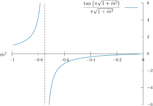
Figure 2: The plot of $\tan\pi\sqrt{1+\hat{m}^{2}}/\pi\sqrt{1+\hat{m}^{2}}$. When $\gamma_{3}>1$, there is only one solution in the range $-1<\hat{m}^{2}<-3/4$.

As shown in Ref. [7], the semiclassical solutions are determined by

$$\gamma_{3}=\frac{\tan\pi\sqrt{1+\hat{m}^{2}}}{\pi\sqrt{1+\hat{m}^{2}}}=\dfrac{\tan\pi p}{\pi p}\,,$$ (3.11)

where $\gamma_{3}$ is the dimensionless parameter

$$\gamma_{3}:=\frac{G_{3}}{G_{4}}\frac{L^{2}}{\pi\ell}\,.$$ (3.12)

Under the Dirichlet boundary condition on $\Sigma_{D}$ and the mixed boundary condition on $\Sigma_{0}$, the non-trivial solution exists only when $\gamma_{3}>1$ in the range $-1<\hat{m}^{2}<-3/4$ ($0<p<1/2$). See Fig. 2. Then, the ratio between $C_{1}$ and $C_{2}$ becomes negative, i.e.,

$$C_{1}C_{2}<0$$ (3.13)

in both the global AdS₃ case and the BTZ case.

4 The boundary free energy

To evaluate the total effective action (2.3), one needs to derive the second variation of the boundary action ${\cal S}_{\text{bdy}}={\cal S}_{\text{EH}}+{\cal S}_{\text{GH}}+{\cal S}_{\text{ct}}$, combined with the bulk calculation (2.27). The $2$-dimensional GH term ${\cal S}_{\text{GH}}$ and the $2$-dimensional counter term ${\cal S}_{\text{ct}}$ are defined by

$${\cal S}_{\text{GH}} =\frac{1}{8\pi G_{3}}\int dtdy\sqrt{-\sigma}\,{\sigma}^{ab}{\mathcal{K}}_{ab}\Big{|}_{u=0}\,,\quad\left(a,\,b=t,\,y\right)$$

$${\cal S}_{\text{ct}} =\frac{\alpha}{16\pi G_{3}}\int dtdy\sqrt{-\sigma}\Big{|}_{u=0}\,,$$ (4.1)

where $\sigma_{ab}:=\mathcal{G}_{ab}$ and ${\mathcal{K}}_{ab}$ is the $2$-dimensional extrinsic curvature given by

$${\mathcal{K}}_{ab}:=-\frac{1}{2N}\partial_{u}{\sigma}_{ab}=-\frac{u\sqrt{f}}{\ell\sqrt{1+\epsilon U}}\partial_{u}{\mathcal{G}}_{ab}\,,$$ (4.2)

and $N$ is the lapse function of the metric (3). Note that the parameter $\alpha$ is to be chosen so that the divergent terms in the total action (2.3) are eliminated. See below (4.15).

The second variation of the boundary Einstein-Hilbert action ${\cal S}_{\text{EH}}$ can be also evaluated via the formulas (A) and (A.4) as

$${\delta^{2}}{\cal S}_{\text{EH}} =\frac{\epsilon^{2}}{16\pi G_{3}}\int_{\Sigma_{0}}d^{3}x\sqrt{-\bar{g}}\Biggl{[}\frac{1}{2}h^{(0)\mu\nu}\left(\bar{D}^{2}+\frac{2}{\ell^{2}}\right)h^{(0)}_{\mu\nu}+\bar{D}_{\mu}V^{\mu}\Biggr{]}$$

$$=\frac{\epsilon^{2}}{32\pi G_{3}}\int_{\Sigma_{0}}d^{3}x\sqrt{-\bar{g}}\,h^{(0)\mu\nu}\left(\bar{D}^{2}+\frac{2}{\ell^{2}}\right)h^{(0)}_{\mu\nu}+{\delta^{2}}{\cal S}_{\text{V}}\,,$$ (4.3)

where $\bar{\mathcal{G}}_{\mu\nu}(x)=\bar{g}_{\mu\nu}(x)$, $\delta\mathcal{G}_{\mu\nu}(x)=h^{(0)}_{\mu\nu}(x):=\lim_{z\to 0}h_{\mu\nu}(z,x)$. Here note that ${\delta^{2}}{\cal S}_{\text{V}}$ is defined on the $2$-dimensional timelike boundary $\partial\Sigma_{0}$ at $u=0$ as

$$\delta^{2}{\cal S}_{\text{V}}=\frac{\epsilon^{2}}{16\pi G_{3}}\int_{\partial\Sigma_{0}}dtdy\sqrt{-\bar{\sigma}}\,\bar{n}_{\mu}V^{\mu}\,,$$ (4.4)

where $n^{\mu}$ is the unit outward vector normal to the boundary $\partial\Sigma_{0}$. Note also that in general there could be some contribution from ${H\cap\Sigma_{0}}$ to $\delta^{2}{\cal S}_{V}$, but in the present case, we do not have such contributions.

From eqs. (2.27) and (4), we obtain the second variation of the total effective action (2.3),

$${\delta^{2}}{\mathcal{S}} =-\frac{\epsilon}{16\pi G_{3}}\int_{\Sigma_{0}}d^{3}x\sqrt{-\bar{g}}h^{(0)\mu\nu}\Biggl{[}-\frac{\epsilon}{2}\left(\bar{D}^{2}+\frac{2}{\ell^{2}}\right)h^{(0)}_{\mu\nu}-8\pi G_{3}\delta\left\langle~{}\mathcal{T}_{\mu\nu}~{}\right\rangle\Biggr{]}$$

$$\quad+{\delta^{2}}{\cal S}_{\text{V}}+{\delta^{2}}{\cal S}_{\text{GH}}+{\delta^{2}}{\cal S}_{\text{ct}}\,.$$ (4.5)

The first and second order variations of ${\cal S}_{\text{GH}}$ and ${\cal S}_{\text{ct}}$ are obtained as

$${\delta\mathcal{S}}_{\text{GH}}=\frac{{\epsilon}}{8\pi G_{3}\ell}\int_{\partial\Sigma_{0}}dtdy\left[-f^{\prime}U+\frac{f}{u}(uU^{\prime}-2U)\right]\,,$$ (4.6)

$${\delta^{2}\mathcal{S}}_{\text{GH}} =\frac{{\,\epsilon^{2}}}{32\pi G_{3}\ell}\int_{\partial\Sigma_{0}}dtdy\Biggl{[}-(1+f)\{T^{2}+2T(U-Y)-(U-Y)(3U+Y)\}$$

$${}\qquad\qquad\qquad+4uf\{(T+U-Y)T^{\prime}+(Y+U-T)Y^{\prime}\}\Biggr{]}\,,$$ (4.7)

and

$${\delta\mathcal{S}}_{\text{ct}}=\frac{{\epsilon}\,\alpha}{16\pi\ell G_{3}}\int_{\partial\Sigma_{0}}dtdy\frac{\sqrt{f}}{u}U\,,$$ (4.8)

$${\delta^{2}\mathcal{S}}_{\text{ct}}=-\frac{{\,\epsilon^{2}}\,\alpha}{32\pi\ell G_{3}}\int_{\partial\Sigma_{0}}dtdy\frac{\sqrt{f}}{u}(T-Y)^{2}\,,$$ (4.9)

where we have used (3) in eqs. (4.6), (4.8), and $f^{\prime}=(f-1)/u$ in eq. (4). Since $U$ behaves near $u=0$ as $U\sim u^{(3-\sqrt{1+\hat{m}^{2}})/2}$ as seen from eqs. (3) and (3), and $-1<\hat{m}^{2}<-3/4$, we find

$${\delta\mathcal{S}}_{\text{GH}}={\delta\mathcal{S}}_{\text{ct}}=0\,.$$ (4.10)

Therefore the surface terms at $O(\epsilon)$ do not appear when one evaluates the on-shell action.

At the second order, $O(\epsilon^{2})$, we obtain

$${\delta^{2}\mathcal{S}}_{\text{V}}+{\delta^{2}\mathcal{S}}_{\text{GH}} =\frac{{\,\epsilon^{2}}}{16\pi G_{3}\ell}\int dtdy\Biggl{[}f(TT^{\prime}+YY^{\prime}-3UU^{\prime})$$

$${}\qquad\qquad+\frac{1}{2u}\{3(1+f)U^{2}-(f-1)(T^{2}-Y^{2})\}+\frac{1+f}{u}TY\Biggr{]}\Biggr{|}_{u\to 0}$$

$$=\frac{{\,\epsilon^{2}}}{16\pi G_{3}\ell}\int dtdy\left\{\frac{1+f}{u}TY-f(TY)^{\prime}\right\}\Biggr{|}_{u\to 0}\,,$$ (4.11)

where we have used (3) and $f^{\prime}=(f-1)/u$ in the second equality. From eqs. (3), (3), and (3), we find that $U$, $T$, and $Y$ asymptotically behave as

$$U\simeq C_{1}u^{\frac{3-p}{2}}+C_{2}u^{\frac{3+p}{2}}\,,$$

$$T\simeq-p(C_{1}u^{\frac{1-p}{2}}-C_{2}u^{\frac{1+p}{2}})\,,$$

$$Y\simeq p(C_{1}u^{\frac{1-p}{2}}-C_{2}u^{\frac{1+p}{2}})\,.$$ (4.12)

Substituting eqs. (4) into eqs. (4) and (4.9), one obtains

$${\delta^{2}\mathcal{S}}_{\text{V}}+{\delta^{2}\mathcal{S}}_{\text{GH}} =\frac{{\,\epsilon^{2}}\,p^{2}}{16\pi G_{3}\ell}\int dtdy\{-C_{1}^{2}(1+p)u^{-p}+2C_{1}C_{2}+O(u^{p})\}\,,$$

$${\delta^{2}\mathcal{S}}_{\text{ct}} =\frac{{\,\epsilon^{2}}\,\alpha p^{2}}{8\pi G_{3}\ell}\int dtdy\{C_{1}^{2}u^{-p}-2C_{1}C_{2}+O(u^{p})\}\,.$$ (4.13)

Thus, the total of the surface terms at $O(\epsilon^{2})$ reduces to a finite term

$${\delta^{2}\mathcal{S}}_{\text{V}}+{\delta^{2}\mathcal{S}}_{\text{GH}}+{\delta^{2}\mathcal{S}}_{\text{ct}}=-\frac{{\,\epsilon^{2}}\,p^{3}}{8\pi G_{3}\ell}\int dtdy\,C_{1}C_{2}\,,$$ (4.14)

if and only if one chooses the parameter $\alpha$ as

$$\alpha=\frac{1+p}{2}\,.$$ (4.15)

Note that $\alpha=1$ when the backreaction from the vacuum expectation value of the stress-energy tensor $\left\langle~{}\mathcal{T}_{\mu\nu}~{}\right\rangle$ is negligible, i.e., when $G_{3}\to 0$ by eqs. (3.11) and (3.12). This is the case for the AdS/CFT correspondence in the $2$-dimensional non-dynamical boundary theory [12]. Note also that the coefficient $\alpha$ in the counter term ${\cal S}_{\text{ct}}$ in eqs. (4) is not determined by the state of the boundary theory, but by the dimensionless parameter $\gamma_{3}$ of the theory via eq. (3.11).

Summarizing the above results all together—in particular, the fact that the semiclassical Einstein equations (2) yields that the integrand of the first line of eq. (4) vanishes, we finally obtain the on-shell value ${\delta^{2}\mathcal{S}^{\text{OS}}}$ of the second order variation of the total effective action (4) as the right-hand side of the total surface terms (4.14).

The deviation ${\Delta}F$ of the free energy of our static semiclassical solutions constructed in Sec. 3 from that of the corresponding (either global AdS₃ or BTZ) background is related to the total effective action by

$${\Delta}F=-{\Delta\mathcal{S}^{\text{OS}}}/\int dt\,=-\left(\mathcal{S}^{\text{OS}}-\bar{\mathcal{S}}^{\text{OS}}\right)/\int dt\,.$$ (4.16)

At $O(\epsilon^{2})$, $\Delta F$ is evaluated as

$${\Delta}F{\,=-\frac{1}{2}\,\delta^{2}\mathcal{S}^{\text{OS}}/\int dt}=\frac{\epsilon^{2}p^{3}}{16\pi G_{3}\ell}\int dy\,C_{1}C_{2}<0$$ (4.17)

by the inequality (3.13). This means that the free energy of the semiclassical solution with $\left\langle~{}\mathcal{T}_{\mu\nu}~{}\right\rangle\neq 0$ is smaller than that of the corresponding (either the global AdS₃ or BTZ) background solution with $\left\langle~{}\mathcal{T}_{\mu\nu}~{}\right\rangle=0$. Therefore the semiclassical AdS₃ solution with vanishing source term is thermodynamically unstable.

5 Summary and discussions

We have investigated thermodynamic instabilities of $3$-dimensional asymptotically AdS solutions to the holographic semiclassical Einstein equations by computing the free energies of the solutions. We have considered AdS₃ with AdS₄ bulk dual as our background solution to the holographic semiclassical Einstein equations with vanishing source term, $\left\langle~{}\mathcal{T}_{\mu\nu}~{}\right\rangle=0$. Then, by considering the tensor-type perturbations with respect to the AdS₄ bulk dual, we have analytically constructed static asymptotically AdS₃ solutions to the semiclassical Einstein equations with non-vanishing CFT source term, $\left\langle~{}\mathcal{T}_{\mu\nu}~{}\right\rangle\neq 0$. These new solutions can be regarded as semiclassical AdS₃ solution with “quantum hair.” We have constructed two such semiclassically hairy AdS₃ solutions: the one with respect to the static BTZ black hole background, which is the same as that found in [7], and the other with respect to the global AdS₃ with no horizon. The free energies of these semiclassically hairy solutions have been evaluated by inspecting the on-shell effective action composed of both the $3$-dimensional Einstein-Hilbert action of the boundary conformal metric and the AdS₄ bulk action. We have shown that the free energy of the semiclassically hairy AdS₃ solution is smaller than that of the AdS₃ solution (with respect to either BTZ black hole chart or the global AdS₃ chart) when the universal parameter $\gamma_{3}$ in (3.12) exceeds the critical value, i.e., $\gamma_{3}>1$.

The existence of such non-trivial AdS solutions with quantum hair reminds us of spontaneous symmetry breaking, in which a less symmetric solution appears from a highly symmetric one when one varies a control parameter of the theory. In our case, the parameter is the universal parameter $\gamma_{3}$ in (3.12), and less symmetric solutions with “quantum hair” appears when $\gamma_{3}$ exceeds the critical value. As discussed in [7], $\gamma_{3}$ is given by the ratio between the magnitude of the stress-energy tensor $\left\langle~{}\mathcal{T}_{\mu\nu}~{}\right\rangle$ composed of the vacuum fluctuations and that of the (classical) stress-energy tensor $\mathcal{T}^{\Lambda}_{\mu\nu}$ composed of the $3$-dimensional cosmological constant. Then, the phase transition is triggered when the vacuum fluctuations overcome the magnitude of $\mathcal{T}^{\Lambda}_{\mu\nu}$. If this effect is universal, one expects that such a spontaneous symmetry breaking should occur, regardless of whether the CFT is strongly coupled or not. It would be interesting to construct semiclassical solutions in the framework of a free CFT in curved spacetime.

One may wonder if such a phase transition occurs for other spacetimes, such as asymptotically flat or de Sitter spacetimes. In asymptotically de Sitter spacetime, for example, one would obtain linearized semiclassical Einstein equations in asymptotically de Sitter spacetime, just like the master equation (3.6). The regularity condition on the black hole horizon or at the center determines the solutions uniquely, except the amplitude. So, one can expect that the linearized solution would be generically singular at the cosmological horizon, and therefore there are no static semiclassical solutions that become asymptotically de Sitter spacetimes. Similarly, one may also expect that asymptotically flat spacetime would not admit any static semiclassical solutions. It would be interesting to consider whether such a no go theorem in asymptotically flat or de Sitter spacetimes holds.

There are other directions to extend the present work. For example, it would be interesting to compare the present result with the braneworld quantum BTZ black hole [15] and its limit toward the conformal boundary of the AdS₄ bulk. It would also be interesting to explore whether the similar type of instabilities found in this paper and associated phase transitions can occur in the case of higher dimensional AdS spacetimes. For example, in $4$ or higher even-dimensional AdS spacetime, there is a trace anomaly, where the length scale in the highly symmetric phase would vary with the universal control parameter, $\gamma_{4}$. Furthermore, in higher dimensional AdS_d black hole with dimension $d>3$, the black hole horizon radius $r_{H}$ would affect the phase transition as a new additional control parameter.

Acknowledgments

We wish to thank Roberto Emparan for useful discussions. We are grateful to the long term workshop YITP-T-23-01 held at YITP, Kyoto University, where a part of this work was done. This work is supported in part by JSPS KAKENHI Grant No. 15K05092, 20K03938 (A.I.), 20K03975 (K.M.), 17K05427(T.O.), and also supported by MEXT KAKENHI Grant-in-Aid for Transformative Research Areas A Extreme Universe No.21H05186 (A.I. and K.M.) and 21H05182.

Appendix A Variation formulas

Under the tensor-type perturbation (2.14), the first order variations are

$$\delta(\sqrt{-\tilde{G}}) =\frac{{\epsilon}}{2}\sqrt{-\bar{g}}\,\bar{g}^{\mu\nu}h_{\mu\nu}=0\,,$$

$$\delta{R}[\tilde{G}] =\epsilon\left(-h_{\mu\nu}\bar{{R}}[{\tilde{G}}]^{\mu\nu}+\bar{\tilde{\nabla}}^{M}\bar{\tilde{\nabla}}^{N}h_{MN}-\bar{\tilde{\nabla}}^{M}\bar{\tilde{\nabla}}_{M}h\right)$$

$$=\epsilon\left(h_{\mu\nu}\frac{2{\mathcal{G}}^{\mu\nu}}{\ell^{2}}+\bar{D}^{\mu}\bar{D}^{\nu}h_{\mu\nu}-\bar{\tilde{\nabla}}^{M}\bar{\tilde{\nabla}}_{M}h\right)=0\,,$$

$$\delta{R}[\tilde{G}]_{\mu\nu} =\epsilon\left(-\frac{1}{2}\bar{\tilde{\nabla}}^{M}\bar{\tilde{\nabla}}_{M}h_{\mu\nu}-\frac{3}{\ell^{2}}h_{\mu\nu}\right)\,,$$ (A.1)

where $\tilde{\nabla}_{M}$ denotes the covariant derivative operator compatible with $\tilde{G}_{MN}$. The second order variations are

$${\delta^{2}}\left(\sqrt{-\tilde{g}}\right) =-\frac{{\epsilon^{2}}}{2}\sqrt{-\bar{g}}h_{\mu\nu}h^{\mu\nu}\,,$$

$$\delta\left(\tilde{\nabla}^{M}\tilde{\nabla}^{N}{\epsilon}\,h_{MN}\right) ={\epsilon^{2}}\sqrt{-\bar{g}}\left[-\frac{1}{2}\left(h^{\mu\nu}h^{\prime}_{\mu\nu}\right)^{\prime}-\bar{D}_{\mu}\left(h^{\nu\alpha}\bar{D}_{\alpha}{h_{\nu}}^{\mu}\right)-\frac{1}{4}\bar{D}_{\mu}\bar{D}^{\mu}\left({h_{\alpha}}^{\beta}{h_{\beta}}^{\alpha}\right)\right]\,,$$

$$\delta\left(\tilde{\nabla}^{M}\tilde{\nabla}_{M}{\epsilon}h\right) =\epsilon^{2}\left\{-\left(h^{\alpha\beta}h_{\alpha\beta}\right)^{\prime\prime}-\bar{D}^{2}\left(h^{\alpha\beta}h_{\alpha\beta}\right)\right\}\,.$$ (A.2)

Substituting these into the second variations of ${R}[\tilde{G}]$, one obtains

$${\delta^{2}}{R}[\tilde{G}]={\epsilon^{2}\bigg{\{}}-\frac{1}{\ell^{2}}h_{\mu\nu}h^{\mu\nu}+\frac{1}{2}h^{\mu\nu}\left(\bar{D}^{2}h_{\mu\nu}+h^{\prime\prime}_{\mu\nu}\right)+\left(h^{\mu\nu}h_{\mu\nu}\right)^{\prime\prime}$$

$${}\qquad{}\qquad\qquad+\frac{3}{4}\bar{D}^{2}\left(h^{\mu\nu}h_{\mu\nu}\right)-\bar{D}_{\mu}\bar{D}_{\nu}\left(h^{\alpha\nu}{h_{\alpha}}^{\mu}\right)-\frac{1}{2}(h^{\mu\nu}h^{\prime}_{\mu\nu})^{\prime}{\bigg{\}}}\,.$$ (A.3)

Similarly, we also obtain the second variation of $\mathcal{R}$ as

$${\delta^{2}}\mathcal{R}={\epsilon^{2}\,\bigg{\{}}\frac{1}{2}h^{\mu\nu}\left(\bar{D}^{2}-\frac{2}{\ell^{2}}\right)h_{\mu\nu}+\frac{3}{4}\bar{D}^{2}\left(h^{\mu\nu}h_{\mu\nu}\right)-\bar{D}_{\mu}\bar{D}_{\nu}\left(h^{\alpha\nu}{h_{\alpha}}^{\mu}\right){\bigg{\}}}\,.$$ (A.4)

References

[1]
G. T. Horowitz and R. M. Wald,
“Dynamics of Einstein’s Equation Modified by a Higher Order Derivative Term,”
Phys. Rev. D 17 (1978), 414-416
[2]
G. T. Horowitz,
“SEMICLASSICAL RELATIVITY: THE WEAK FIELD LIMIT,”
Phys. Rev. D 21, 1445-1461 (1980)
[3]
W. M. Suen,
“Minkowski Space-time Is Unstable in Semiclassical Gravity,”
Phys. Rev. Lett. 62 (1989), 2217-2220
[4]
A. A. Starobinsky,
“A New Type of Isotropic Cosmological Models Without Singularity,”
Phys. Lett. B 91 (1980), 99-102
[5]
A. Vilenkin,
“Classical and Quantum Cosmology of the Starobinsky Inflationary Model,”
Phys. Rev. D 32 (1985), 2511
[6]
G. Compere and D. Marolf,
“Setting the boundary free in AdS/CFT,”
Class. Quant. Grav. 25, 195014 (2008)
doi:10.1088/0264-9381/25/19/195014
[arXiv:0805.1902 [hep-th]].
[7]
A. Ishibashi, K. Maeda and T. Okamura,
“Semiclassical Einstein equations from holography and boundary dynamics,”
JHEP 05 (2023), 212
[arXiv:2301.12170 [hep-th]].
[8]
J. M. Maldacena,
“The Large N limit of superconformal field theories and supergravity,”
Adv. Theor. Math. Phys. 2 (1998), 231-252
[arXiv:hep-th/9711200 [hep-th]].
[9]
S. S. Gubser, I. R. Klebanov and A. M. Polyakov,
“Gauge theory correlators from noncritical string theory,”
Phys. Lett. B 428 (1998), 105-114
[arXiv:hep-th/9802109 [hep-th]].
[10]
E. Witten,
“Anti-de Sitter space and holography,”
Adv. Theor. Math. Phys. 2 (1998), 253-291
[arXiv:hep-th/9802150 [hep-th]].
[11]
S. de Haro, S. N. Solodukhin and K. Skenderis,
“Holographic reconstruction of space-time and renormalization in the AdS / CFT correspondence,”
Commun. Math. Phys. 217, 595-622 (2001)
[arXiv:hep-th/0002230 [hep-th]].
[12]
V. Balasubramanian and P. Kraus,
“A Stress tensor for Anti-de Sitter gravity,”
Commun. Math. Phys. 208 (1999), 413-428
[arXiv:hep-th/9902121 [hep-th]].
[13]
J. Z. Simon,
“The Stability of flat space, semiclassical gravity, and higher derivatives,”
Phys. Rev. D 43, 3308-3316 (1991)
[14]
J. Z. Simon,
“No Starobinsky inflation from selfconsistent semiclassical gravity,”
Phys. Rev. D 45, 1953-1960 (1992)
[15]
R. Emparan, A. M. Frassino and B. Way,
“Quantum BTZ black hole,”
JHEP 11, 137 (2020)
[arXiv:2007.15999 [hep-th]].