Event-Based Contrastive Learning for Medical Time Series

Abstract

In clinical practice, one often needs to identify whether a patient is at high risk of adverse outcomes after some key medical event; for example, the short-term risk of death after an admission for heart failure. This task is challenging due to the complexity, variability, and heterogeneity of longitudinal medical data, especially for individuals suffering from chronic diseases like heart failure. In this paper, we introduce Event-Based Contrastive Learning (EBCL), a method for learning embeddings of heterogeneous patient data that preserves temporal information before and after key index events. We demonstrate that EBCL produces models that yield better fine-tuning performance on critical downstream tasks for a heart failure cohort, including 30-day readmission, 1-year mortality, and 1-week length of stay, relative to other pretraining methods. Our findings also reveal that EBCL pretraining alone can effectively cluster patients with similar mortality and readmission risks, offering valuable insights for clinical decision-making and personalized patient care.

1 Introduction

A central feature of many predictive tasks in medicine is that one aspires to identify a patient’s risk of a future adverse event after some index event, such as an inpatient admission or a diagnostic test like echocardiography. Prediction of such risks is important for the development of effective treatment strategies (Rahimi et al., 2014) and for ensuring that healthcare resources are allocated appropriately (Duong et al., 2021; Jencks et al., 2009). This has motivated researchers to study a variety of learning algorithms, including directly supervised (Zhang et al., 2021; Rajkomar et al., 2018), self-supervised (Tipirneni & Reddy, 2022; Labach et al., 2023) and contrastive learning algorithms (Hyvarinen & Morioka, 2017; Agrawal et al., 2022) for the identification of patients at the highest risk of adverse outcomes. Specifically, contrastive learning algorithms - a class of representation learning methods - (Raghu et al., 2023; Jeong et al., 2023; Diamant et al., 2022; King et al., 2023) define latent space structure through positive and negative pairs—where positive pairs of points should be close and negative far apart in the latent space.

Many of these contrastive learning methods (and more generally representation learning) for medical time series data (Agrawal et al., 2022; Tipirneni & Reddy, 2022; Labach et al., 2023), strive to create latent representations that preserve temporal trends within the data. These methods, however, generally ignore the fact that some portions of medical time series data are more informative than others. For example, data surrounding clinically important index events (e.g., an admission for a heart attack, or an admission associated with a new cancer diagnosis) are rich in information that plays a significant role in patient prognostication.

Our approach, Event-Based Contrastive Learning (EBCL), diverges from existing work (Hyvarinen & Morioka, 2017; Agrawal et al., 2022; Dave et al., 2022) by imposing a specialized pretraining contrastive loss solely on data around critical events, where the most clinically-relevant information regarding disease progression and prognosis is likely to be found. In particular, we use patient data immediately before and after a key medical event as positive pairs, and data from different patients as negative pairs (Figure 1). The resulting embedding maps data surrounding key medical events to similar regions of the latent space, thereby encoding temporal trends.

We evaluate EBCL on a multi-center cohort of heart failure patients and perform empirical comparisons with state-of-the-art published pretraining systems for the medical domain on three outcome prediction tasks, including 30-day readmission, 1-year mortality, and 1-week length of stay (LOS) prediction. We present finetuning results that show that EBCL consistently outperforms these baselines across all tasks. Furthermore, beyond traditional fine-tuning, we also show that EBCL embeddings produce much more informative representations of patient state, achieving linear probing AUCs at least $5.46$ points higher than other methods for predicting Mortality and $16.78$ points for predicting LOS. EBCL further yields highly expressive clusters, suggesting capabilities for patient sub-typing. Via ablation studies, we demonstrate that the advantages of EBCL are uniquely due to its focus on temporal trends surrounding key medical events. Overall, our results strongly demonstrate the benefits of the domain-specific latent space structure EBCL learns through its focus on key medical events and its unique temporal contrastive loss formulation. In summary, our contributions are as follows:

• We propose a new contrastive pretraining method for time series data that encodes patient-specific temporal trends around key medical events in clinical data.

• We demonstrate that this formalism leads to improved predictive performance on downstream outcome prediction tasks, consistently outperforming published pretraining baselines and supervised models.

• EBCL pretraining alone generates embeddings that are useful for identifying high risk subgroups based on patient-specific temporal trends. This suggests these contrastive pretraining methods may be useful beyond downstream task prediction and for patient subtyping.

2 Related Works

Representation Learning for Clinical Time-Series Data

Medical time series datasets pose unique challenges due to their inherently high-dimensional and irregularly sampled nature, and the significant presence of missing data (Shukla & Marlin, 2020). These complexities demand focused strategies to encode (Tipirneni & Reddy, 2022) and represent such time-series data (Li & Marlin, 2020; Tipirneni & Reddy, 2022; Lee et al., 2023; McDermott et al., 2023a; Labach et al., 2023) to enhance model performance, particularly in scenarios with limited data. Decision tree baselines, such as XGBoost (Chen & Guestrin, 2016) remain competitive for both tabular and tabular time series data (Labach et al., 2023; Shwartz-Ziv & Armon, 2021), while many pretraining methods have been explored, which includes pretraining methods such as forecasting (STraTS) (Tipirneni & Reddy, 2022) and masked imputation (DueTT) (McDermott et al., 2021; Labach et al., 2023), and weakly supervised (McDermott et al., 2021). More recently, contrastive learning methods (Agrawal et al., 2022; Hyvarinen & Morioka, 2017; King et al., 2023) have been applied to time series and multimodal temporal data, which is known to impose deeper structural constraints on latent space geometry (McDermott et al., 2023b) motivating them as a better option for the pretraining objectives. We focus on advancing contrastive learning methods for time series to impose and leverage meaningful latent space structures for downstream tasks.

Time-Aware Contrastive Learning Recent work has applied contrastive learning to time series data, specifically a scheme called Order Contrastive Pretraining (OCP) (Agrawal et al., 2022). OCP takes two consecutive windows of data in their original temporal sequence to construct positive pairs. Negative pairs correspond to a sequence where the temporal order of sequences is swapped (Figures 3, 5). Importantly, the sequences chosen to be swapped are not chosen with respect to any particular event in prior applications (Agrawal et al., 2022; Hyvarinen & Morioka, 2017). However, we hypothesize OCP would not have strength in detecting the changes in static features (e.g., persistent low left ventricular ejection fraction in heart failure patients) across time as all the views agree on constant features in a patient. This stresses the need for the views that could represent such differences between patients.

3 Event-Based Contrastive Learning (EBCL) for Medical Time-Series

Figure 1: Event-based contrastive learning (EBCL). For patient $i$ and event $j$, we denote pre-event data, $L_{i}^{j}$, and post-event data, $R_{i}^{j}$. For EBCL pretraining, we sample a batch, $\mathcal{B}$, of pre and post-event trajectory pairs from a dataset, $D_{\mathcal{B}}=\{(L_{i}^{j},R^{i}_{j}):i,j\in\mathcal{B}\}$. We choose the event of interest to be an inpatient admission. $L_{i}^{j}$ and $R_{i}^{j}$ are passed separately into a transformer encoder $f_{\theta}$ to get $\bar{L}_{i}^{j}=f_{\theta}(L_{i}^{j})$ and $\bar{R}_{i}^{j}=f_{\theta}(R_{i}^{j})$ which is pretrained with CLIP contrastive loss. The positive pairs are pre and post-event data of the same event, $(\bar{L}_{i}^{j},\bar{R}_{i}^{j})$. The negative pairs are mismatched pre-event and post-event trajectories from different patients, such as $(\bar{L}_{i}^{j},\bar{R}_{l}^{m})$ where $i\neq l$.

3.1 Problem Formulation

Let $\mathcal{D}$ be a dataset containing $N$ patient trajectories, $\{X_{1},\cdots,X_{N}\}$. A patient trajectory $X_{i}=[x_{i,1},x_{i,2},\ldots,x_{i,M_{i}}]$ is a chronologically ordered sequence of patient $i$’s $M_{i}\in\mathbb{N}$ observations. Each observation $x_{i,j}$ corresponds to an individual medical event (e.g., a laboratory test) and is encoded as a triple $x_{i,j}=(t_{i,j},o_{i,j},v_{i,j})$ where $t_{i,j}$ is the time of the observation, $o_{i,j}$ denotes what medical result is being measured (e.g., what lab test is being observed), and $v_{i,j}$ is the actual value of the observation. For example, if a patient has a potassium test (encoded via $o=7$) taken at time $t=\text{``12/1/2022, 11:30 a.m.''}$ which reports a value of 4.2 mEq/L, then their corresponding patient trajectory would contain a triple $(t_{i,j},o_{i,j},v_{i,j})=(\text{``2/1/2024, 8:00 a.m.''},7,4.2)$.

To define the patient windows that EBCL will contrast during pre-training, we define the following. Given a window size $\tau\in\mathbb{N}$, let $t_{i,j}$ be the timestamp of a clinical index event (e.g., a hospital admission) and define $L_{i}^{j}\subset X_{i}$ to be a subset of patient $i$’s trajectory consisting of the $\tau$ events prior to $t_{i,j}$ and $R_{i}^{j}\subset X_{i}$ be the subsequent $\tau$ events including and after $t_{i,j}$:

$$L_{i}^{j} =[x_{i,j-\tau},x_{i,j-\tau+1},\ldots,x_{i,j-1}]$$

$$R_{i}^{j} =[x_{i,j},x_{i,j+1},\ldots,x_{i,j+\tau-1}].$$

3.2 Model Optimization Pipeline

We consider a two-stage learning problem where we pretrain a network $f_{\theta}$ and fine-tune on the outcome prediction tasks that are of interest.

EBCL Pretraining

For pretraining a model, we sample an event and its corresponding pre-event and post-event dataset. We use a model, $f_{\theta}$ as an encoder, and get pre- and post-embeddings $f_{\theta}(L_{i}^{j})$ and $f_{\theta}(R_{i}^{j})$. We then compute the CLIP loss $\mathcal{L}\textsubscript{CLIP}$ (Radford et al., 2021) on a batch of these embeddings, where $(L_{i}^{j},R_{l}^{m})$ is a positive pair if $i=l$ and $j=m$. Intuitively, CLIP loss pushes together representations of positive pairs (i.e. paired left and right windows) and repels representations of negative pairs (i.e. mismatched left and right windows) as depicted in Figure 1.

Finetuning

During fine-tuning, we use encoder $f_{\theta}$ to get representations finetuned for downstream outcome classification task. We use negative cross-entropy loss, $\mathcal{L}\textsubscript{CE}$, and pass our embeddings, $f_{\theta}(L_{i}^{j})$ and $f_{\theta}(R_{i}^{j})$ through a shallow feedforward network (see Appendix Figure 8) to arrive at a prediction for our label, $y_{i}^{j}$. EBCL weights after pretraining are used to initialize this model for the downstream tasks defined in Section 4.1. For the LOS task, we only use the pre-representation $f_{\theta}(L_{i}^{j})$ and pass that to the shallow feedforward network, and post data would leak the target.

4 Dataset and Experimental Setting

In this section, we introduce the dataset, outcome prediction tasks, and baseline models we used for the experiment.

4.1 Dataset

We have assembled a multi-center cohort of $107,268$ patients with a prior diagnosis of heart failure. Collectively, this cohort had $383,254$ inpatient admissions, obtained from the electronic data warehouse of a large hospital network. The dataset includes patient trajectories over a maximum span of $40$ years and a maximum number of $3,275$ features, which includes labs, diagnoses, procedures, medications, tabular echocardiogram recordings, physical measurements (weight, height), and admissions/discharges. In our heart failure cohort, we restrict our clinical events to inpatient admissions that have at least $16$ data points for both pre-admission and post-admission data. If a patient has no such event, they were not included in the cohort. We partitioned our compiled dataset into training (80%), validation (10%), and testing (10%) with the split stratified so that no patients overlapped across splits. Additional information on dataset preprocessing is provided in the appendix Section B.

Table 1: Statistics for finetuning datasets.

Task	# Patients	# Events	# Prevalence
30-Day Readmission	65,435	262,734	26.8%
1-Year Mortality	52,748	195,747	30.6%
1-Week LOS	107,268	383,254	54.1%

4.2 Tasks

We finetune and evaluate on three binary downstream tasks: 30-day readmission, 1-year mortality, and 7-day LOS). The datasets are summarized in Table 1. Note that for the LOS task, we only use Pre-Admission data as input, as Post-Admission data would leak the LOS outcome. We also always restrict Post-Admission data, $R_{n}^{i}$, to the data prior to patient discharge, as this is the information that will be available at decision time for the 1-year mortality and 30-day readmission tasks.

4.3 Model Architecture

For all experiments, unless specified otherwise, we use a transformer encoder as the backbone of our architecture (Figure 8). The encoder has two encoder layers with the input of 512 observation sequences followed by a 128-dimension feed-forward layer between self-attention layers, and 32-dimension token embeddings. We then perform Fusion Self-Attention (Tipirneni & Reddy, 2022; Raffel & Ellis, 2016), by taking an attention-weighted average of the output embeddings of the transformer to get a single 32-dimension embedding. Finally, we have a linear projection to a 32-dimension embedding. Input sequences are required to have a length of at least 16 observations and are padded to be length of 512. Attention over padded tokens is masked in the transformer and the Fusion Self-Attention layer. This is the exact architecture from the paper (Tipirneni & Reddy, 2022) except we use a 128 dimension feed-forward layer instead of 2048 as this improved the supervised baselines in initial experiments.

4.4 Baseline methods

To evaluate our method, we perform experiments with the following baselines and dataset preparation methods. For more information on methods, see Appendix Section B.

XGBoost (Chen & Guestrin, 2016): XGBoost is a tree boosting-based machine learning algorithm, widely used for classification and regression tasks with tabular datasets, and a competitive baseline for time-series prediction tasks (McDermott et al., 2023a).

Supervised Transformer (S-Trans): This corresponds to standard supervised training without EBCL pretraining. The transformer model $f_{\theta}$ is initialized with random weights, and then the model is trained in a supervised fashion for a specific task.

Order Contrastive Pretraining (OCP) (Agrawal et al., 2022): We pretrain $f_{\theta}$ with the OCP objective where for each patient $i$, we take a continuous sequence of at most 512 tokens, split the sequence in half, and randomly swap the first and second halves (Appendix Figure 5).

Self-supervised Transformer for Time-Series (STraTS) (Tipirneni & Reddy, 2022): STraTS represents transformer-based forecasting of time-series data. The transformer-based architecture they proposed is designed for handling sparse and irregularly sampled multivariate clinical time-series data.

Dual Event Time Transformer (DuETT) (Labach et al., 2023): DueTT proposes a masked imputation pretraining task for detecting the presence of a feature and its value.

4.5 Finetuning and Downstream Outcome Prediction

We finetune the pretrained models (OCP, STraTS, DueTT, and EBCL) with a single fully connected layer to predict outcomes. We perform an extensive learning rate and dropout hyperparameter search for pretraining and finetuning and use a maximum of 300 epochs for pretraining and 100 epochs for finetuning. More details are provided in the Appendix Section B.2. We take the epoch with the highest validation set performance for pretraining and finetuning. We pretrain our models and run 5 random seeds for finetuning and report the mean and standard deviation of results across these seeds and compare results for statistical significance via a $t$-test.

Table 2: EBCL Pretraining improves results over a supervised baseline and time-series pretraining baselines. We summarize the downstream finetuning performance using both the area under the receiver operating characteristic (AUC) and the area under the precision-recall curve (APR) of three prediction tasks (30-Day Readmission, 1-Year Mortality, and 1-Week Length of Stay (LOS)) averaged over 5 runs with different seeds. Across all tasks, EBCL results (bolded) were statistically significantly better than all other tested models.

	30-Day Readmission		1-Year Mortality		1-Week LOS
	AUC	APR	AUC	APR	AUC	APR
XGBoost	70.85 $\pm$ 0.08	86.19 $\pm$ 0.03	80.33 $\pm$ 0.19	89.58 $\pm$ 0.08	79.74 $\pm$ 0.10	79.79 $\pm$ 0.08
S-Trans	70.28 $\pm$ 0.16	85.60 $\pm$ 0.12	81.54 $\pm$ 0.24	90.27 $\pm$ 0.15	88.74 $\pm$ 0.48	88.61 $\pm$ 0.48
OCP (Agrawal et al., 2022)	70.27 $\pm$ 0.32	85.48 $\pm$ 0.20	80.06 $\pm$ 0.29	89.36 $\pm$ 0.18	90.06 $\pm$ 0.25	90.05 $\pm$ 0.28
STraTS (Tipirneni & Reddy, 2022)	70.06 $\pm$ 0.11	85.45 $\pm$ 0.07	79.95 $\pm$ 0.62	89.31 $\pm$ 0.43	88.36 $\pm$ 1.09	87.73 $\pm$ 2.03
DueTT (Labach et al., 2023)	69.51 $\pm$ 0.50	85.51 $\pm$ 0.31	79.39 $\pm$ 0.16	89.04 $\pm$ 0.11	75.35 $\pm$ 0.61	74.66 $\pm$ 0.62
EBCL	71.66 $\pm$ 0.03	86.40 $\pm$ 0.03	82.43 $\pm$ 0.07	90.55 $\pm$ 0.03	90.98 $\pm$ 0.05	90.96 $\pm$ 0.04

Table 3: Linear Probing for Evaluating the Pretrained Embeddings. Across all tasks, EBCL results (bolded) were the best performing embeddings.

	30-Day Readmission		1-Year Mortality		1-Week LOS
	AUC	APR	AUC	APR	AUC	APR
OCP	65.78 $\pm$ 0.36	83.02 $\pm$ 0.31	71.24 $\pm$ 0.40	83.56 $\pm$ 0.37	60.33 $\pm$ 0.29	56.36 $\pm$ 0.42
STraTS	63.11 $\pm$ 0.37	81.22 $\pm$ 0.34	67.15 $\pm$ 0.42	81.05 $\pm$ 0.41	57.75 $\pm$ 0.30	53.28 $\pm$ 0.41
DuETT	59.54 $\pm$ 0.39	78.94 $\pm$ 0.36	64.71 $\pm$ 0.43	78.56 $\pm$ 0.43	57.43 $\pm$ 0.30	51.62 $\pm$ 0.39
EBCL	67.6 $\pm$ 0.36	83.94 $\pm$ 0.30	76.70 $\pm$ 0.36	87.59 $\pm$ 0.29	77.11 $\pm$ 0.24	76.96 $\pm$ 0.29

5 Experiments and Results

Now that we have defined our model and dataset, we present the following key results: 1) EBCL outperforms all baselines on fine-tuning tasks. 2) EBCL yields richer embeddings than competitor pretraining models. 3) The definition of the domain-informed event and its closeness to the sampled event are key to our performance gains.

5.1 EBCL Outperforms All Baselines on All three Finetuning Downstream Tasks

Our proposed method, EBCL, achieves a significant improvement over all baselines (Table 2) in predicting all three tasks (1-Year Mortality, 30-Day Readmission, 1-Week Length of Stay (LOS)). We note that pretraining methods can often achieve improved performance relative to a supervised baseline when the pretraining dataset is significantly larger than the finetuning datasets (Devlin et al., 2019; Dosovitskiy et al., 2021). However, in this case, EBCL achieves better performance over the supervised baseline even though the pretraining and finetuning datasets are of similar size. Consequently, the improvement in performance arises from solving the contrastive learning task and not the fact that pretraining leverages a larger dataset. Our experiment confirms our hypothesis that contrasting around our index event better captures temporal trends than other contrastive and generative pretraining methods.

Each time-series pretraining baseline model learns distinct features that, in principle, help the model perform better for subsequent finetuning clinical outcome classification task. XGBoost builds a representation that summarizes information along the long period of clinical time series. OCP (Agrawal et al., 2022) learns features that are sensitive to temporal reversal (which are called least time reversible features). STraTS (Tipirneni & Reddy, 2022) is designed to learn features that are useful for forecast observations during inpatient stays, which helps build a representation that captures relevant features and temporal dependencies. DueTT (Labach et al., 2023) representation learns missingness-invariant representations of data from masked imputation for accurate downstream prediction robust to missingness of input pretraining data. By contrast, EBCL learns patient-specific temporal trends associated with inpatient admissions (the clinical index event in this application).

5.2 Embeddings from EBCL Pretrained model are More Informative than Other Baselines

Linear Probing

To gauge the extent to which the pretrained embeddings captured pertinent features for a specific classification task, we employed a linear probing evaluation. This involved fitting a logistic regression classifier on the fixed embeddings generated by the model, which helped assess the representational capacity of our pretrained model. The coefficient for L2 regularization was tuned. To obtain standard deviations for linear probing results, we use bootstrapping: we sample with replacement $1,000$ bootstraps from the testing dataset, and report mean and standard deviation in table 3.

EBCL representations consistently outperformed other baseline methods for all three tasks evaluated. We see dramatic improvements when using a KNN classifier as well (results and methodology are in Appendix Section C). This implies that neighbors within the EBCL latent space are more similar in outcomes than those derived from any other baseline model. This suggests that, solely through pretraining, EBCL inherently learns a structure that stratifies outcomes.

Patient Subtyping with EBCL Representations

Figure 2: Clustering and outcome risk subtyping from pretrained EBCL Embedding. (a)-(c) Clustering and dimensionality reduction of pretrained embedding showed distinct heart failure subgroups with unique outcome prognoses: Healthier group with longer years to mortality, later readmission (blue group) and Fatal group with shorter years to mortality, earlier readmission (Pink group). ((d)-(e) The subgroups of heart failure patients identified with EBCL showed markedly more distinct phenotypes compared to other baselines.

We compare the utility of embeddings from all pretrained models for clustering patients into groups with similar outcomes. From the EBCL pretrained transformer, we build pre-event and post-event vector representations for each admission in the test set to form a concatenated transformer embedding that includes comprehensive information pre- and post-event. We use $K$-means clustering with $k=2$ on this embedding space to effectively identify distinct subgroups of heart failure cohorts with different prognoses. We use dimensional reduction with Uniform Manifold Approximation and Projection (UMAP) (McInnes et al., 2020) for the ease of visualization of our high-dimensional data. The identified clusters that were found are superimposed over the resulting UMAP graphic to highlight the separation and distribution of the clusters in the reduced-dimensional space in Figure 2 (a). To understand the phenotype of each cluster, we compare the outcome of patients in each identified cluster (years to mortality, days to readmission, the prevalence of 1-year mortality, and 30-day readmission) (Figure 2). To further validate the prognostic differentiation between the identified heart failure subgroups, we plotted Kaplan-Meier (KM) (Dudley et al., 2016) survival curves of the patients in each cluster in figure 2 (b) and (c). This approach allowed us to visually and statistically compare the distribution of time-to-event of patients in the clusters.

EBCL Embeddings Cluster Patients with Statistically Significantly Different Time-To-Event Distributions

The resulting EBCL clusters correspond to two distinct patient subgroups, each having markedly different prognoses, as illustrated in Figure 2. Cluster 2 presented a heart failure subgroup of more critical conditions with higher 1-year mortality (50.87%) and 30-day readmission (23.52 %) rate. Furthermore, cluster 2 presented a shorter time to mortality with a shorter duration to readmission (Figure 2, time to death, time to readmission plot (pink)). In contrast, cluster 1 presented a subgroup with a healthier prognosis, evidenced by lower outcome prevalence (50.87 % died within a year, 34.53 % were readmitted within 30 days), longer time to death, and extended durations to the next inpatient admission (Figure 2, time to death, time to readmission plot (blue)). We find a significant difference in the time-to-event KM curve of both mortality and readmission between the clusters using a $t$-test with p-value $0.01$.

EBCL Embeddings Cluster Patients into More Distinct Outcome Clusters Than Our Baselines

For EBCL and our Baselines, we compute the absolute difference in percent prevalence between clusters for Mortality and Readmission in Figures 2 (d) and (e). We find that EBCL pretrained embeddings are able to identify distinct subtypes of heart failure patients with worse prognoses compared to other baselines.

5.3 Ablation Studies

Performance Gains Observed with EBCL were Uniquely due to Key Event and Closeness of Data

Table 4: Ablation Studies. We compare the EBCL variants by applying various definitions of events and different sampling strategies. We summarize the downstream finetuning performance (AUROC, AUPRC) of three prediction tasks averaged over 5 runs with different seeds, where we boldface statistically significant results. * Note that FT stands for finetuning data and the entry both means both pre and post data are used, but for predicting 1-Week LOS we always only used the Pre-event dataset to avoid data leakage.

			30-Day Readmission		1-Year Mortality		1-Week LOS
	Index Event	FT*	AUC	APR	AUC	APR	AUC	APR
EBCL	Inpatient	Both	71.66 $\pm$ 0.03	86.40 $\pm$ 0.03	82.43 $\pm$ 0.07	90.55 $\pm$ 0.03	90.98 $\pm$ 0.05	90.96 $\pm$ 0.04
Censoring	Inpatient	Both	70.63 $\pm$ 0.10	85.83 $\pm$ 0.04	81.35 $\pm$ 0.04	90.08 $\pm$ 0.02	90.43 $\pm$ 0.11	90.35 $\pm$ 0.12
Non-Adm	Non-Inpatient	Both	70.73 $\pm$ 0.11	85.75 $\pm$ 0.05	81.89 $\pm$ 0.10	90.45 $\pm$ 0.06	90.12 $\pm$ 0.17	90.06 $\pm$ 0.18
Outpatient	Outpatient	Both	70.51 $\pm$ 0.14	85.66 $\pm$ 0.11	81.80 $\pm$ 0.03	90.34 $\pm$ 0.02	89.68 $\pm$ 0.14	89.64 $\pm$ 0.12
Pre Event	Inpatient	Pre	70.48 $\pm$ 0.09	85.70 $\pm$ 0.06	79.63 $\pm$ 0.06	88.89 $\pm$ 0.05	✗	✗
Post Event	Inpatient	Post	69.20 $\pm$ 0.09	85.11 $\pm$ 0.06	80.36 $\pm$ 0.03	89.41 $\pm$ 0.01	✗	✗

The novelty of our method arises from 1) leveraging the clinically important event and 2) using the data around the index event. We perform a series of ablation studies to analyze the effect of defining the event and sampling observations around the event.

Effect of the definition of event

We evaluate the importance of selecting a clinically significant event for pretraining by selecting non-inpatient admission events. We first use any non-inpatient visits as the EBCL index event (such as outpatient visits or emergency unit visits) instead of inpatient admission (Non-Adm EBCL). Our standard EBCL model, which uses inpatient hospital admission as the index event, outperformed an approach that specifically excludes inpatient admissions from the event set (Table 4).

As the Non-Adm EBCL experiments include encounters with the emergency room, we also performed a second set of experiments where events were restricted to only outpatient encounters (thereby excluding all emergency department encounters). These Outpatient EBCL experiments also underperformed standard EBCL. These results highlight the critical role of inpatient admissions in learning consistent patterns for predicting clinically significant outcomes, suggesting that the context around inpatient events is essential for optimal model performance in this cohort.

Effect of Censoring Observations

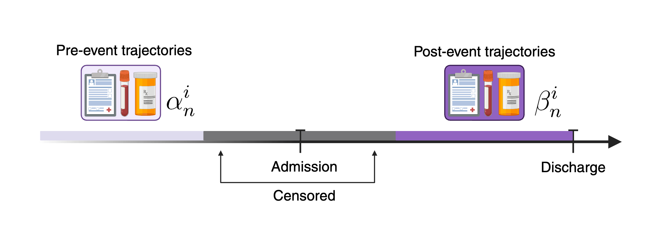
Figure 10: EBCL - Censoring Ablation. We censor a fixed number of observations from the end of the pre window and beginning of the post window and take the 512 remaining closest observations before the admission as pre data and after the admission and post data.

We evaluate the importance of sampling observations locally around the index event by introducing a censoring window around the EBCL inpatient admission index event (EBCL with Censoring). In this experiment, we sample consecutive input observation points that are away from the index event by setting the censoring window (Appendix Figure 10). Pre-event observations were chosen from the window preceding the censoring window before the index event. Post-event observations were chosen from the window following the censoring window after the index event. EBCL with Censoring demonstrated lower performance compared to the standard EBCL (Table 4). This outcome reinforces the fundamental advantage of EBCL, which capitalizes on the proximity of data around the index event. Hence, leveraging data close to the index event is crucial for the model’s effectiveness in clinical prediction tasks.

Effect of Finetuning with Only Pre-event or Post-event Data

To determine whether the gains of EBCL are primarily driven by data before or after the index event data, we evaluated our performance when the input was limited to either data before the index event (pre) or after the index event (post). Limiting the dataset only to pre-event or post-event data yields worse performance for downstream tasks compared to using both inputs (Table 4). In addition, DueTT(Labach et al., 2023) and STraTS(Tipirneni & Reddy, 2022) baselines were originally proposed with ICU data as the target application. ICU data is more densely populated than outpatient data and corresponds most closely to the post-inpatient admission windows in our experiments. We therefore performed Pre Event and Post Event experiments on all our baselines to test whether using only post-event (or pre-event) data would improve the performance of DueTT or STraTS relative to EBCL. However, these experiments demonstrate that EBCL consistently outperforms these other methods regardless of whether inputs are restricted to post-event or pre-event data (Table 6, 7).

6 Discussion

EBCL, a novel pretraining scheme for medical time series data, learns patient-specific temporal representations around clinically significant events. We demonstrate that the method outperforms previous contrastive, generative, and supervised baselines through finetuning results. We further show that EBCL pretraining generates a rich latent space characterized by: 1) significant improvements in classification performance with linear probing on EBCL latent space and 2) improvement in identifying high risk patient subgroups using embeddings arising from EBCL pretraining alone. From a set of ablation studies, we show that the key to performance gains in EBCL is from the introduction of the event and the nearness of data around that index event.

In the current application, we apply the method to a cohort of patients with a prior diagnosis of heart failure, where hospital admission is the clinically significant event of interest. Heart failure provides a particularly good application domain because the trajectory of patients with heart failure is punctuated by frequent hospital admissions, where each admission is associated with a further decrease in myocardial function (Gheorghiade et al., 2005); i.e., hospital admissions are particularly important in the health trajectory of these patients. Our findings, which are limited to a singular dataset, allow us to evaluate the method in a controlled environment, applying it to a disorder associated with significant morbidity and mortality. Our results motivate future experiments applying EBCL to different clinical and non-clinical time series datasets. In particular, most, if not all, chronic disorders are similarly associated with events representing significant changes in clinical trajectory; e.g., an admission for diabetic ketoacidosis, sickle cell crisis in a patient with sickle cell disease, etc. Moreover, as EBCL contrasts windows of data around an event, there is nothing in the formalism that restricts its application to any particular data type. Indeed, the application to multi-modal time series is straightforward in that it only necessitates the use of appropriate embeddings for each modality. This flexibility signifies its potential as a universal tool for multi-modal time series.

7 Broader Impact

The potential broader impacts of EBCL are considerable and varied. First, for the specific application discussed in this paper, we demonstrate that EBCL pretraining can be used to enhance our ability to identify heart failure patients who are at high risk of 30-day readmission, death within 1-year and those who will have a prolonged length of stay. Generally, the ability to accurately identify the occurrence of such high risk events facilitates the optimal allocation of healthcare resources, ensuring timely care for patients at the highest risk of adverse events (Duong et al., 2021; Jencks et al., 2009). In addition, embeddings arising from unsupervised EBCL pretraining identifies patients at high risk of death within one-year after a hospital admission. The ability to identify such high risk patient subgroups remains a major challenge in clinical cardiology, hence these results represents a significant advance in this area.

Secondly, EBCL introduces methodological innovations into the pretraining process, by limiting the pretraining loss to regions of the medical time series that are associated with key index events. This approach not only enhances the application of EBCL to complex time series data but also opens avenues for its adoption across various other domains, demonstrating the method’s versatility and potential for broad impact.

8 Acknowledgements

We would like to thank members of the Computational Cardiovascular Research Group and HealthyML Lab at MIT for their invaluable feedback.

Appendix A Views of Contrastive Learning

In this section, we outline the contrastive learning framework of EBCL and its variations compared to the contrastive baseline (OCP (Agrawal et al., 2022)) and specify some examples of what information they learn throughout pretraining. Our proposed method (EBCL) takes positive and negative samples (A, B) or (C, D) from the same patient’s medical record, where window A or C immediately precedes window B or D in time in the original medical record. Furthermore, windows A and C immediately precede a key medical event (e.g., inpatient admission), and windows B and D immediately follow that same key medical event in the original medical record. EBCL uses negative sample pairs (A, D) or (C, B) from different patients’ medical records, where, for instance, A immediately precedes a key medical event and D immediately follows a key medical event in the original medical record. Our EBCL variants (EBCL Censored, EBCL Outpatients) follow the same definition for selecting positive and negative pairs, where we censor some windows around the index event (EBCL Censored) or select different index event (EBCL Outpatients). On the contrary, OCP takes the swapped sequence (N, M) from the same patient to become the negative sample and the original ordered sequence (M, N) becomes the positive sample.

Figure 3: Contrastive Learning Framework of EBCL, EBCL Ablations (EBCL Censored, EBCL Outpatient) and OCP.

Due to this difference inherently arising from the definition of positive and negative samples, OCP (Agrawal et al., 2022) and EBCL have distinct potential for learning different types of features in a medical record. We can think of two different features that have $x_{1}$ a static nature that doesn’t change frequently over time and $x_{2}$ a time-varying feature that changes over a short period of time. Under OCP pre-training, the value of feature $x_{1}$ is identical over two consecutive windows M and N. Thus, OCP pre-training cannot use the observed value of the feature to differentiate between a positive pair (M, N) and a negative pair (N, M) as both pairs agree on the feature value, so the model is not incentivized to capture the approximate value of the static feature in the produced embeddings at all. For EBCL, the value of the static feature agrees between positive samples, as it originates from the same patient. However, the value of the feature will disagree in the negative sample. Therefore, the EBCL model is incentivized to capture the approximate value of static features in its embeddings.

Let’s now think about a feature that oscillates over time, which stays centered near a constant value, but oscillates with local temporal trends across both patients. Under OCP pretraining, the model can see that the trends observed in window M will directly continue into window N, which gives a strong signal that (M, N) is an appropriately ordered pair. In contrast, for a swapped sequence, the model will see that the trends do not continue from N to M, which clearly indicates an incorrectly ordered pair. Thus, this will be a strong signal for the model to differentiate positive (correctly ordered) from negative (incorrectly ordered) pairs, so the model will be incentivized to capture the local trends of oscillating features within windows M and N. Under EBCL pretraining, much like in OCP, the model can see that the trends observed in window A will directly continue into window B, which gives a strong signal that (A, B) is an appropriately ordered pair within the same patient. In contrast, for the negative pair (A, D) the model will be much less likely to observe a non-continuing pattern, which will be a clear negative signal. So, similar to OCP, the model is incentivized to capture the local trends of features within windows A and B in its embeddings. This is under the assumption that the feature is likely to be observed and retain its locally oscillatory behavior both near key events and distant from key events.

Appendix B Dataset and Experimental Setting

Figure 4: XGBoost requires a fixed size vector as input. We create this vector from time series data as follows: we restrict to the 128 most prevalent features in the data and the relative time of those observations (relative to the time of the decision). For each of the time windows prior to the time of the decision (discharge time for 1-Year Mortality and 30-Day Readmission and admission time for 7-Day LOS). Perform feature aggregations (mean, count, min value, max value) for each feature over all pre-defined time windows. We then concatenate all of the feature aggregation outputs across all windows to get a final vector that is the input to XGBoost. We have 5 window sizes and 4 aggregations for our 129 length vector, leading to a 2580 size vector that is the input for XGBoost.

Figure 5: OCP Positive and Negative Pairs. In OCP, positive pairs are sequences with correct order, while negative pairs have the order of the first and second halves of the timeline swapped. The model, $f_{\theta}$ is pretrained to predict whether the sequence was swapped.

Figure 6: STraTS forecast patient trajectory in the forecasting window and is trained with Mean Squared Error (MSE) loss calculated on the observations present in the forecasting window.

Figure 7: DueTT(Labach et al., 2023) bins data into 32 time bins and a finite number of events as is depicted on the left side. For our admissions data this corresponds to binning data from the patient’s first observation to their discharge time (or admission time for the LOS task). The pretraining task is to mask out a row (an event) and a column (a time bin) and predict the event values and event presences for the masked blocks.

B.1 Dataset Preprocessing

We preprocess our heart failure dataset as follows: features with less than $1,000$ occurrences in the entire dataset are dropped. Categorical values with less than $1,000$ occurrences are replaced with the categorical value “UNKNOWN”. We use the triplet embedding strategy from (Tipirneni & Reddy, 2022) for modeling sequential EHR data, and this allows flexibility in how dates are encoded. For all experiments, we encode dates as the relative time in days from the inpatient admission event divided by the standard deviation of these times in the training set. We label encode categorical observation values and features, and z normalize continuous data and feed it into a continuous value embedder to get a vector.

B.2 Model Architecture and Training

Figure 8 summarizes the model architecture used for pretraining and finetuning for EBCL, OCP, STraTS, and fully supervised experiments.

Figure 8: Model Architectures. FFN refers to a one hidden layer feed-forward network. (a) This architecture is used for EBCL, OCP, STraTS, and Supervised experiments. For EBCL we initialize $\theta$ with the final weights from EBCL pretraining, $\theta^{*}_{\mathrm{EBCL}}$, for OCP we initialize with the final weights from OCP pretraining, $\theta^{*}_{\mathrm{OCP}}$, and for Supervised we randomly initialize $\theta$. Notice that Pre-event data and Post-event data are passed separately into the transformer encoder $f_{\theta}$, so there is no self-attention between Pre-event and Post-event data. (b) Architecture used for OCP Pretraining. The binary label for computing the cross entropy loss, $\mathcal{L}\textsubscript{CE}$, is whether or not the random sequence, $\tau^{i}$, is swapped. (c) Architecture used for EBCL Pretraining. The ”Pre Projection” and ”Post Projection” are linear projections, and their weights are not shared.

Hyperparameter tuning

For both our pretraining and finetuning, we perform the same hyperparameter search with $16$ pairs. Learning rates are sampled from the log uniform distribution ($1e-6$, $1e-2$), and dropouts are sampled from the uniform distribution ($0$, $0.6$). We use the ASHA scheduler (Li et al., 2020) with a grace period of $4$ epochs and a reduction factor of $2$ to schedule the training of these jobs and select the trial with the best final validation loss. The ASHA scheduler will halt trials early in training that have a very high loss relative to other trials. Additionally, we use an early stopping tolerance of $3$ epochs for all experiments.

B.3 XGBoost

For the preparation of input dataset for XGBoost, we selected the 128 most prevalent features in our dataset and added the 129th feature for the relative time of these observations from admissions. We aggregate summary statistics (average, minimum, maximum) of the dataset within different windows (1 day, 1 week, 1 month, 1 year, $\infty$ years) from the decision date (Figure 4). For a fair comparison, we limit XGBoost to the same observations available in the EBCL pre and post windows (Table 2).

B.4 Order Contrastive Pretraining (Agrawal et al., 2022)

We prepare a continuous trajectory of 512 consecutive data points. This trajectory might either be maintained in its original order or have its two halves swapped (Figure 5. For the case where we keep the original ordering, the last data point, $T_{256}$, is set to time $0$, with subsequent data points indicating the time elapsed since $T_{256}$. Alternatively, if we swap the trajectory, the last data point of the latter half, $T_{512}$, becomes time $0$. Other data points then denote the time difference from $T_{512}$. We further adjust the dates of the initial half by adding the time gap, $T\textsubscript{GAP}=T_{512}-T_{256}$. This adjustment ensures that the gap between $T_{256}$ and $T_{257}$ remains unaltered, regardless of whether the sequence is swapped or not.

For OCP pretraining we use the same transformer model as the EBCL experiments use, and for finetuning the same EBCL finetuning architecture displayed in figure 8 (a). Due to slow convergence, we allow up to a maximum of 300 epochs for pretraining. For fine-tuning, we load the OCP pretrained weights into our finetuning architecture in Figure 8.

B.5 STraTS (Tipirneni & Reddy, 2022)

STraTS represents time series as observation triplets, utilizing Continuous Value Embedding for time, feature, and values, and incorporates self-supervised learning for better generalization in data-limited scenarios. We implement the STraTS forecasting strategy for our dataset by randomly sampling a forecasting window with at least one observation in it and 16 observations prior to it. We use the median inpatient length of stay, 6 days, as our forecasting window length. All observations prior to the forecasting window (cutoff at a maximum of 512) are in our input window, and the STraTS pretraining task is to predict the data values in the prediction window. We calculate the Mean Squared Error (MSE) loss between features present in the forecast window with the forecasted output, as shown in Figure 6.

The input window is all data randomly sampled before the forecast window of 6 days, where we have at least 1 observation in the forecast window and 16 in the input window. All observations before the forecasting window (cutoff at a maximum of 512) are in our input window, and the pretraining task is to predict the data values in the prediction window, and the loss is computed over the subset of values that are observed in the prediction window (Figure 6). We use the same relative times as described for the original sequence in the OCP experiment. For STraTS pretraining we use the same transformer model as the EBCL experiments use, and for finetuning the same EBCL finetuning architecture (Figure 8 (a)).

B.6 DueTT (Labach et al., 2023)

We select the $128$ most prevalent features in the dataset and bin the dataset into 32-time bins. We augment this two-dimensional matrix of input data with 128 features and 32-time bins by stacking the same size of the input matrix with the count of each feature within each time bin. We use 2 transformer encoder layers over the time dimension and two over the feature dimensions, as performed in the DueTT paper. See Appendix Figure 7 for a visual. We generally achieved the best performance pretraining on timebins covering pre and post-data combined, even when we finetuned on only pre or post-data, such as for the LOS task. For producing embeddings, we use a DueTT model pretrained on time bins covering pre and post-data. We generate a pre-embedding by inputting only pre admission data and averaging the output tensor over the 128 feature dimensions and 32 time bin dimensions to get a single 24 dimensional pre data vector. We get a 24-dimensional post embedding the same way.

Appendix C KNN

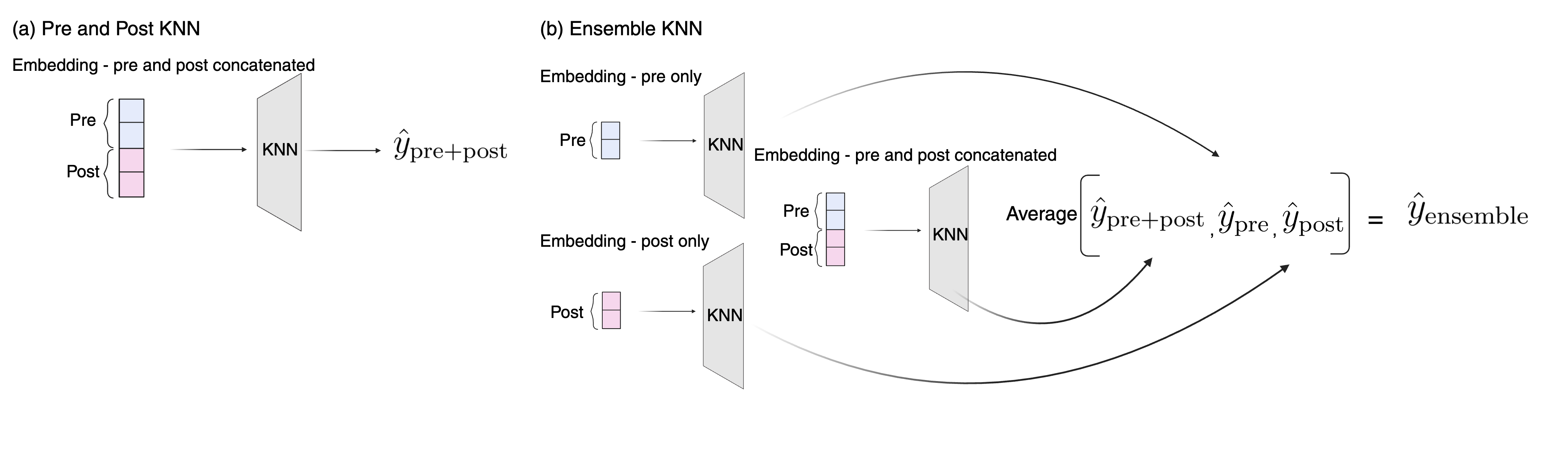
Figure 9: KNN Models. We try two KNN classifier strategies. The Pre and Post model concatenates the pre and post window representations before feeding them into the KNN. The Ensemble model averages the predicted class probabilities from three KNNs where: (1) $\hat{y}\textsubscript{pre}=$ class probabilities from a KNN retrieving pre representation neighbors, (2) $\hat{y}\textsubscript{post}=$ class probabilities from a KNN retrieving post representation neighbors, or (3) $\hat{y}\textsubscript{pre+post}=$ class probabilities from a KNN retrieving neighbors of the concatenated pre and post representation.

Table 5: K-Nearest Neighbors for Evaluating the Pretrained Embeddings. We boldface the best results.

	30-Day Readmission		1-Year Mortality		1-Week LOS
	AUC	APR	AUC	APR	AUC	APR
OCP (Agrawal et al., 2022)	67.46 $\pm$ 0.36	84.00 $\pm$ 0.30	72.61 $\pm$ 0.39	84.68 $\pm$ 0.35	64.51 $\pm$ 0.29	61.90 $\pm$ 0.39
STraTS (Tipirneni & Reddy, 2022)	60.49 $\pm$ 0.37	79.95 $\pm$ 0.34	64.06 $\pm$ 0.43	78.77 $\pm$ 0.41	57.84 $\pm$ 0.30	53.57 $\pm$ 0.41
DuETT (Labach et al., 2023)	59.71 $\pm$ 0.38	79.32 $\pm$ 0.34	64.32 $\pm$ 0.42	78.06 $\pm$ 0.43	57.17 $\pm$ 0.30	53.16 $\pm$ 0.40
EBCL	68.46 $\pm$ 0.36	84.89 $\pm$ 0.28	77.87 $\pm$ 0.34	88.21 $\pm$ 0.28	81.59 $\pm$ 0.22	81.66 $\pm$ 0.25

For our KNN Classifier experiments, we do a sweep over all combinations of the following parameters:

1. Neighbor Weighting: uniform or distance

2. KNN Model: Pre-and-Post or ensemble

3. Distance Metrics Cosine distance, Euclidean, or Euclidean with pre and post embeddings individually L2 normalized.

4. Number of Neighbors 10, 30, 100, 300, and 1000

For neighbor weighting, we either weigh the labels of neighbors uniformly or by the inverse of their distance. We detail KNN models in Figure 9. The tasks that use pre and post-representations (1-Year Mortality and 30-Day Readmission) use either of two KNN classifier models. For the Pre and Post KNN model, the pre and post-representations are concatenated, and we fit a KNN classifier on these concatenated embeddings. For the Ensemble KNN model, we average the class probabilities from a Pre and Post, a pre-only, and a post-only KNN classifier. Note that for the 1-Week LOS task, we use only a pre-only KNN model. For each model’s embeddings, we select the hyperparameter combination with the best validation set performance and report the test set performance of this configuration. We achieve similar results to linear probing and again observe that EBCL significantly outperforms other baselines. Moreover, this analysis reveals that neighbors within the EBCL latent space are more similar in outcomes than those derived from any other baseline model, suggesting that EBCL inherently learns an outcome-related clustering structure through pretraining alone.

Appendix D Ablations

D.1 Effect of Sampling Observations

The censoring window length was determined based on the EBCL window statistics analysis. Specifically, we selected the window to align with the 25th percentile for pre-event and post-event observations, according to the EBCL statistics. Excluding the 25th percentile of data preceding and following the event onset led to the exclusion of 260 observations pre-event and 60 observations post-event.

Table 6: Results for finetuning only using pre-admission (Pre-event) data.

	30-Day Readmission		1-Year Mortality
	AUC	APR	AUC	APR
XGBoost	69.86 $\pm$ 0.03	85.35 $\pm$ 0.02	77.27 $\pm$ 0.04	87.76 $\pm$ 0.02
Supervised	68.27 $\pm$ 0.16	84.37 $\pm$ 0.15	77.36 $\pm$ 0.19	87.42 $\pm$ 0.20
OCP (Agrawal et al., 2022)	68.83 $\pm$ 0.13	84.63 $\pm$ 0.08	77.93 $\pm$ 0.13	87.85 $\pm$ 0.04
STraTS (Tipirneni & Reddy, 2022)	68.46 $\pm$ 0.04	84.34 $\pm$ 0.18	78.18 $\pm$ 0.63	87.89 $\pm$ 0.52
DueTT (Labach et al., 2023)	68.23 $\pm$ 0.11	84.97 $\pm$ 0.03	75.14 $\pm$ 0.37	86.17 $\pm$ 0.23
EBCL	70.48 $\pm$ 0.09	85.70 $\pm$ 0.06	79.63 $\pm$ 0.06	88.89 $\pm$ 0.05

Table 7: Results for finetuning only using post-admission (Post-event) data.

	30-Day Readmission		1-Year Mortality
	AUC	APR	AUC	APR
XGBoost	68.05 $\pm$ 0.10	84.80 $\pm$ 0.04	77.12 $\pm$ 0.17	87.54 $\pm$ 0.16
Supervised	68.68 $\pm$ 0.08	84.69 $\pm$ 0.05	79.77 $\pm$ 0.21	88.92 $\pm$ 0.19
OCP (Agrawal et al., 2022)	68.49 $\pm$ 0.10	84.59 $\pm$ 0.05	79.23 $\pm$ 0.13	88.58 $\pm$ 0.07
STraTS (Tipirneni & Reddy, 2022)	67.61 $\pm$ 0.16	84.05 $\pm$ 0.10	79.60 $\pm$ 0.12	88.71 $\pm$ 0.10
DueTT (Labach et al., 2023)	67.47 $\pm$ 0.09	84.14 $\pm$ 0.06	76.47 $\pm$ 0.74	87.15 $\pm$ 0.35
EBCL	69.20 $\pm$ 0.09	85.11 $\pm$ 0.06	80.36 $\pm$ 0.03	89.41 $\pm$ 0.01

Appendix E Risk Stratification and Patient Subtyping with EBCL

Table 8: Comparative Analysis of One-Year Mortality and 30-Day Readmission Rates Across Patient Clusters Derived from Different Embedding Strategies. Note that the one-year mortality prevalence in the test data is 31.09%. The 30-Day readmission prevalence is 26.66%.

	1-Year Mortality (%)			30 Days Readmission (%)
Cluster	Cluster 1	Cluster 2	$\Delta$ prevalence	Cluster 1	Cluster 2	$\Delta$ prevalence
OCP	23.46	33.18	9.72	19.86	28.43	8.57
STraTS	30.96	31.64	0.68	26.25	28.75	2.50
DueTT	28.07	34.16	6.09	25.09	27.96	2.87
EBCL	28.00	50.87	22.87	23.52	34.53	11.01

We initialized the model with the pretrained model weights of all baseline models (EBCL, OCP (Agrawal et al., 2022), STraTS (Tipirneni & Reddy, 2022), DueTT (Labach et al., 2023)) and concatenated the pre- and post-event embeddings of the test set patients. We applied UMAP (McInnes et al., 2020) to reduce the dimensionality of the embeddings and to easily visualize our high dimensional data. Furthermore, we applied K-means clustering with $k=2$ on the pretrained embeddings to subgroup the patient cohort by outcome risk. Using the identified clusters, we evaluated the survival outcomes with the Kaplan-Meier estimator (Dudley et al., 2016), which provided a visual representation of the survival probability over time for each cluster. To quantitatively compare the prognosis of two identified clusters (Cluster 1 and 2), we compare days to mortality and days to readmission between Cluster 1 and Cluster 2 (Figure 2, Table 8).

Our analysis revealed statistically significant disparities in outcome prevalence among the clusters identified by various predictive models, including EBCL, OCP (Agrawal et al., 2022), and STraTS (Tipirneni & Reddy, 2022). Specifically, using a two-sampled Student’s t-test, we found that Cluster 2 in the EBCL model demonstrated a statistically significant higher one-year mortality rate at 50.87 compared to 28.00 in Cluster 1 (Table 8). This trend was consistent across other models, with the EBCL model showing the highest gaps in prevalence, reinforcing its robustness in stratifying patient risk. However, the clusters identified with STraTS (Tipirneni & Reddy, 2022) on the 1-Year Mortality task didn’t show patient subgroups that are with statistically significantly different prognoses.

Notably, the EBCL model showed better stratification of patients, evidenced by high gaps of prevalence between clusters compared to other baselines (22.87 for one-year mortality and 11.01 for 30-day readmission tasks, respectively. (Table 8, $\Delta$ prevalence column), Figure 2 (d), (e)). These insights demonstrate the capacity of EBCL to generate clinically meaningful representations, potentially aiding in more effective patient stratification and personalized healthcare based on patient phenotyping.

References

- Agrawal et al. (2022) Agrawal, M. N., Lang, H., Offin, M., Gazit, L., and Sontag, D. Leveraging time irreversibility with order-contrastive pre-training. In International Conference on Artificial Intelligence and Statistics, pp. 2330–2353. PMLR, 2022.
- Chen & Guestrin (2016) Chen, T. and Guestrin, C. Xgboost: A scalable tree boosting system. In Proceedings of the 22nd acm sigkdd international conference on knowledge discovery and data mining, pp. 785–794, 2016.
- Dave et al. (2022) Dave, I., Gupta, R., Rizve, M. N., and Shah, M. TCLR: Temporal contrastive learning for video representation. Computer Vision and Image Understanding, 219:103406, jun 2022. doi: 10.1016/j.cviu.2022.103406. URL https://doi.org/10.1016%2Fj.cviu.2022.103406.
- Devlin et al. (2019) Devlin, J., Chang, M.-W., Lee, K., and Toutanova, K. Bert: Pre-training of deep bidirectional transformers for language understanding, 2019.
- Diamant et al. (2022) Diamant, N., Reinertsen, E., Song, S., Aguirre, A. D., Stultz, C. M., and Batra, P. Patient contrastive learning: A performant, expressive, and practical approach to electrocardiogram modeling. PLoS computational biology, 18(2):e1009862, 2022.
- Dosovitskiy et al. (2021) Dosovitskiy, A., Beyer, L., Kolesnikov, A., Weissenborn, D., Zhai, X., Unterthiner, T., Dehghani, M., Minderer, M., Heigold, G., Gelly, S., Uszkoreit, J., and Houlsby, N. An image is worth 16x16 words: Transformers for image recognition at scale, 2021.
- Dudley et al. (2016) Dudley, W. N., Wickham, R., and Coombs, N. An introduction to survival statistics: Kaplan-meier analysis. Journal of the advanced practitioner in oncology, 7(1):91, 2016.
- Duong et al. (2021) Duong, S. Q., Zheng, L., Xia, M., Jin, B., Liu, M., Li, Z., Hao, S., Alfreds, S. T., Sylvester, K. G., Widen, E., et al. Identification of patients at risk of new onset heart failure: Utilizing a large statewide health information exchange to train and validate a risk prediction model. Plos one, 16(12):e0260885, 2021.
- Gheorghiade et al. (2005) Gheorghiade, M., De Luca, L., Fonarow, G. C., Filippatos, G., Metra, M., and Francis, G. S. Pathophysiologic targets in the early phase of acute heart failure syndromes. The American Journal of Cardiology, 96(6):11–17, September 2005. ISSN 0002-9149. doi: 10.1016/j.amjcard.2005.07.016. URL http://dx.doi.org/10.1016/j.amjcard.2005.07.016.
- Hyvarinen & Morioka (2017) Hyvarinen, A. and Morioka, H. Nonlinear ICA of Temporally Dependent Stationary Sources. In Singh, A. and Zhu, J. (eds.), Proceedings of the 20th International Conference on Artificial Intelligence and Statistics, volume 54 of Proceedings of Machine Learning Research, pp. 460–469. PMLR, 20–22 Apr 2017. URL https://proceedings.mlr.press/v54/hyvarinen17a.html.
- Jencks et al. (2009) Jencks, S. F., Williams, M. V., and Coleman, E. A. Rehospitalizations among patients in the medicare fee-for-service program. New England Journal of Medicine, 360(14):1418–1428, 2009.
- Jeong et al. (2023) Jeong, H., Stultz, C. M., and Ghassemi, M. Deep metric learning for the hemodynamics inference with electrocardiogram signals. Machine Learning for Healthcare, 54:1–28, 2023.
- King et al. (2023) King, R., Yang, T., and Mortazavi, B. J. Multimodal pretraining of medical time series and notes. In Hegselmann, S., Parziale, A., Shanmugam, D., Tang, S., Asiedu, M. N., Chang, S., Hartvigsen, T., and Singh, H. (eds.), Proceedings of the 3rd Machine Learning for Health Symposium, volume 225 of Proceedings of Machine Learning Research, pp. 244–255. PMLR, 10 Dec 2023. URL https://proceedings.mlr.press/v225/king23a.html.
- Labach et al. (2023) Labach, A., Pokhrel, A., Huang, X. S., Zuberi, S., Yi, S. E., Volkovs, M., Poutanen, T., and Krishnan, R. G. Duett: Dual event time transformer for electronic health records. arXiv preprint arXiv:2304.13017, 2023.
- Lee et al. (2023) Lee, K., Lee, S., Hahn, S., Hyun, H., Choi, E., Ahn, B., and Lee, J. Learning missing modal electronic health records with unified multi-modal data embedding and modality-aware attention. arXiv preprint arXiv:2305.02504, 2023.
- Li et al. (2020) Li, L., Jamieson, K., Rostamizadeh, A., Gonina, E., Hardt, M., Recht, B., and Talwalkar, A. A system for massively parallel hyperparameter tuning, 2020.
- Li & Marlin (2020) Li, S. C.-X. and Marlin, B. Learning from irregularly-sampled time series: A missing data perspective. In International Conference on Machine Learning, pp. 5937–5946. PMLR, 2020.
- McDermott et al. (2021) McDermott, M., Nestor, B., Kim, E., Zhang, W., Goldenberg, A., Szolovits, P., and Ghassemi, M. A comprehensive ehr timeseries pre-training benchmark. In Proceedings of the Conference on Health, Inference, and Learning, pp. 257–278, 2021.
- McDermott et al. (2023a) McDermott, M., Nestor, B., Argaw, P., and Kohane, I. Event stream gpt: A data pre-processing and modeling library for generative, pre-trained transformers over continuous-time sequences of complex events. arXiv preprint arXiv:2306.11547, 2023a.
- McDermott et al. (2023b) McDermott, M. B., Yap, B., Szolovits, P., and Zitnik, M. Structure-inducing pre-training. Nature Machine Intelligence, pp. 1–10, 2023b.
- McInnes et al. (2020) McInnes, L., Healy, J., and Melville, J. Umap: Uniform manifold approximation and projection for dimension reduction, 2020.
- Radford et al. (2021) Radford, A., Kim, J. W., Hallacy, C., Ramesh, A., Goh, G., Agarwal, S., Sastry, G., Askell, A., Mishkin, P., Clark, J., et al. Learning transferable visual models from natural language supervision. In International conference on machine learning, pp. 8748–8763. PMLR, 2021.
- Raffel & Ellis (2016) Raffel, C. and Ellis, D. P. W. Feed-forward networks with attention can solve some long-term memory problems, 2016.
- Raghu et al. (2023) Raghu, A., Chandak, P., Alam, R., Guttag, J., and Stultz, C. Sequential multi-dimensional self-supervised learning for clinical time series. 2023.
- Rahimi et al. (2014) Rahimi, K., Bennett, D., Conrad, N., Williams, T. M., Basu, J., Dwight, J., Woodward, M., Patel, A., McMurray, J., and MacMahon, S. Risk prediction in patients with heart failure: a systematic review and analysis. JACC: Heart Failure, 2(5):440–446, 2014.
- Rajkomar et al. (2018) Rajkomar, A., Oren, E., Chen, K., Dai, A. M., Hajaj, N., Hardt, M., Liu, P. J., Liu, X., Marcus, J., Sun, M., et al. Scalable and accurate deep learning with electronic health records. NPJ digital medicine, 1(1):18, 2018.
- Shukla & Marlin (2020) Shukla, S. N. and Marlin, B. M. A survey on principles, models and methods for learning from irregularly sampled time series. arXiv preprint arXiv:2012.00168, 2020.
- Shwartz-Ziv & Armon (2021) Shwartz-Ziv, R. and Armon, A. Tabular data: Deep learning is not all you need, 2021.
- Tipirneni & Reddy (2022) Tipirneni, S. and Reddy, C. K. Self-supervised transformer for sparse and irregularly sampled multivariate clinical time-series. ACM Transactions on Knowledge Discovery from Data (TKDD), 16(6):1–17, 2022.
- Zhang et al. (2021) Zhang, X., Zeman, M., Tsiligkaridis, T., and Zitnik, M. Graph-guided network for irregularly sampled multivariate time series. arXiv preprint arXiv:2110.05357, 2021.