Online Restless Multi-Armed Bandits with Long-Term Fairness Constraints

Shufan Wang, Guojun Xiong, Jian Li
Abstract

Restless multi-armed bandits (RMAB) have been widely used to model sequential decision making problems with constraints. The decision maker (DM) aims to maximize the expected total reward over an infinite horizon under an โ€œinstantaneous activation constraintโ€ that at most $B$ arms can be activated at any decision epoch, where the state of each arm evolves stochastically according to a Markov decision process (MDP). However, this basic model fails to provide any fairness guarantee among arms. In this paper, we introduce RMAB-F, a new RMAB model with โ€œlong-term fairness constraintsโ€, where the objective now is to maximize the long-term reward while a minimum long-term activation fraction for each arm must be satisfied. For the online RMAB-F setting (i.e., the underlying MDPs associated with each arm are unknown to the DM), we develop a novel reinforcement learning (RL) algorithm named Fair-UCRL. We prove that Fair-UCRL ensures probabilistic sublinear bounds on both the reward regret and the fairness violation regret. Compared with off-the-shelf RL methods, our Fair-UCRL is much more computationally efficient since it contains a novel exploitation that leverages a low-complexity index policy for making decisions. Experimental results further demonstrate the effectiveness of our Fair-UCRL.

Introduction

The restless multi-armed bandits (RMAB) model (Whittle 1988) has been widely used to study sequential decision making problems with constraints, ranging from wireless scheduling (Sheng, Liu, and Saigal 2014; Cohen, Zhao, and Scaglione 2014), resource allocation in general (Glazebrook, Hodge, and Kirkbride 2011; Larraรฑaga, Ayesta, and Verloop 2014; Borkar, Ravikumar, and Saboo 2017), to healthcare (Bhattacharya 2018; Mate, Perrault, and Tambe 2021; Killian, Perrault, and Tambe 2021). In a basic RMAB setting, there is a collection of $N$ โ€œrestlessโ€ arms, each of which is endowed with a state that evolves independently according to a Markov decision process (MDP) (Puterman 1994). If the arm is activated at a decision epoch, then it evolves stochastically according to one transition kernel, otherwise according to a different transition kernel. RMAB generalizes the Markovian multi-armed bandits (Lattimore and Szepesvรกri 2020) by allowing arms that are not activated to change state, which leads to โ€œrestlessโ€ arms, and hence extends its applicability. For simplicity, we refer to a restless arm as an arm in the rest of the paper. Rewards are generated with each transition depending on whether the arm is activated or not. The goal of the decision maker (DM) is to maximize the expected total reward over an infinite horizon under an โ€œinstantaneous activation constraintโ€ that at most $B$ arms can be activated at any decision epoch.

However, the basic RMAB model fails to provide any guarantee on how activation will be distributed among arms. This is also a salient design and ethical concern in practice, including mitigating data bias for healthcare (Mate, Perrault, and Tambe 2021; Li and Varakantham 2022a) and societal impacts (Yin etย al. 2023; Biswas etย al. 2023), providing quality of service guarantees to clients in network resource allocation (Li, Liu, and Ji 2019), just to name a few. In this paper, we introduce a new RMAB model with fairness constraints, dubbed as RMAB-F to address fairness concerns in the basic RMAB model. Specifically, we impose โ€œlong-term fairness constraintsโ€ into RMAB problems such that the DM must ensure a minimum long-term activation fraction for each arm (Li, Liu, and Ji 2019; Chen etย al. 2020; Dโ€™Amour etย al. 2020; Li and Varakantham 2022a), as motivated by aforementioned resource allocation and healthcare applications. The DMโ€™s goal now is to maximize the long-term reward while satisfying not only โ€œinstantaneous activation constraintโ€ in each decision epoch but also โ€œlong-term fairness constraintโ€ for each arm. Our objective is to develop low-complexity reinforcement learning (RL) algorithms with order-of-optimal regret guarantees to solve RMAB-F without knowing the underlying MDPs associated with each arm.

Though online RMAB has been gaining attentions, existing solutions cannot be directly applied to our online RMAB-F. First, existing RL algorithms including state-of-the-art colored-UCRL2 (Ortner etย al. 2012) and Thompson sampling methods (Jung and Tewari 2019; Akbarzadeh and Mahajan 2022), suffer from an exponential computational complexity and regret bounds grow exponentially with the size of state space. This is because those need to repeatedly solve Bellman equations with an exponentially large state space for making decisions. Second, though much effort has been devoted to developing low-complexity RL algorithms with order-of-optimal regret for online RMAB, many challenges remain unsolved. For example, multi-timescale stochastic approximation algorithms (Fu etย al. 2019; Avrachenkov and Borkar 2022) suffer from slow convergence and have no regret guarantee. Adding to these limitations is the fact that none of them were designed with fairness constraints in mind, e.g., (Wang, Huang, and Lui 2020; Xiong, Li, and Singh 2022; Xiong, Wang, and Li 2022; Xiong etย al. 2022; Xiong and Li 2023) only focused on minimizing costs in RMAB, while the DM in our RMAB-F faces a new dilemma on how to manage the balance between maximizing the long-term reward and satisfying both instantaneous activation constraint and long-term fairness requirements. This adds a new layer of difficulty to designing low-complexity RL algorithms with order-of-optimal regret for RMAB that is already quite challenging.

To tackle this new dilemma, we develop Fair-UCRL, a novel RL algorithm for online RMAB-F. On one hand, we provide the first-ever regret analysis for online RMAB-F, and prove that Fair-UCRL ensures sublinear bounds (i.e., $\tilde{\mathcal{O}}(\sqrt{T})$) for both the reward regret (suboptimality of long-term rewards) and the fairness violation regret (suboptimality of long-term fairness violation) with high probability. On the other hand, Fair-UCRL is computationally efficient. This is due to the fact that Fair-UCRL contains a novel exploitation that leverages a low-complexity index policy for making decisions, which differs dramatically from aforementioned off-the-shelf RL algorithms that make decisions via solving complicated Bellman equations. Such an index policy in turn guarantees that the instantaneous activation constraint can be always satisfied in each decision epoch. To the best of our knowledge, Fair-UCRL is the first model-based RL algorithm that simultaneously provides (i) order-of-optimal regret guarantees on both the reward and fairness constraints; and (ii) a low computational complexity, for RMAB-F in the online setting. Finally, experimental results on real-world applications (resource allocation and healthcare) show that Fair-UCRL effectively guarantees fairness for each arm while ensures good regret performance.

Model and Problem Formulation

In this section, we provide a brief overview of the conventional RMAB, and then formally define our RMAB-F as well as the online settings considered in this paper.

Restless Multi-Armed Bandits

A RMAB problem consists of a DM and $N$ arms (Whittle 1988). Each arm $n\in\mathcal{N}=\{1,...,N\}$ is described by a unichain MDP $M_{n}$ (Puterman 1994). Without loss of generality (W.l.o.g.), all MDPs $\{M_{n},\forall n\in\mathcal{N}\}$ share the same finite state space $\mathcal{S}$ and action space $\mathcal{A}:=\{0,1\}$, but may have different transition kernels Pnโ€‹(sโ€ฒ|s,a)subscript๐‘ƒ๐‘›conditionalsuperscript๐‘ โ€ฒ๐‘ ๐‘ŽP_{n}(s^{\prime}|s,a) and reward functions rnโ€‹(s,a)subscript๐‘Ÿ๐‘›๐‘ ๐‘Žr_{n}(s,a), โˆ€s,sโ€ฒโˆˆ๐’ฎ,aโˆˆ๐’œformulae-sequencefor-all๐‘ superscript๐‘ โ€ฒ๐’ฎ๐‘Ž๐’œ\forall s,s^{\prime}\in\mathcal{S},a\in\mathcal{A}. Denote the cardinalities of $\mathcal{S}$ and $\mathcal{A}$ as $S$ and $A$, respectively. The initial state is chosen according to the initial state distribution $\boldsymbol{s}_{0}$ and $T$ is the time horizon. At each time/decision epoch $t$, the DM observes the state of each arm $n$, denoted by snโ€‹(t)subscript๐‘ ๐‘›๐‘กs_{n}(t), and activates a subset of $B$ arms. Arm $n$ is called active when being activated, i.e., $a_{n}(t)=1$, and otherwise passive, i.e., $a_{n}(t)=0.$ Each arm $n$ generates a stochastic reward rnโ€‹(t):=rnโ€‹(snโ€‹(t),anโ€‹(t))assignsubscript๐‘Ÿ๐‘›๐‘กsubscript๐‘Ÿ๐‘›subscript๐‘ ๐‘›๐‘กsubscript๐‘Ž๐‘›๐‘กr_{n}(t):=r_{n}(s_{n}(t),a_{n}(t)), depending on its state snโ€‹(t)subscript๐‘ ๐‘›๐‘กs_{n}(t) and action $a_{n}(t)$. W.l.o.g., we assume that $r_{n}\in[0,1]$ with mean rยฏnโ€‹(s,a),โˆ€n,s,asubscriptยฏ๐‘Ÿ๐‘›๐‘ ๐‘Žfor-all๐‘›๐‘ ๐‘Ž\bar{r}_{n}(s,a),\forall n,s,a, and only active arms generate reward, i.e., rnโ€‹(s,0)=0,โˆ€n,ssubscript๐‘Ÿ๐‘›๐‘ 00for-all๐‘›๐‘ r_{n}(s,0)=0,\forall n,s. Denote the sigma-algebra generated by random variables {(snโ€‹(ฯ„),anโ€‹(ฯ„)),โˆ€n,ฯ„<t}subscript๐‘ ๐‘›๐œsubscript๐‘Ž๐‘›๐œfor-all๐‘›๐œ๐‘ก\{(s_{n}(\tau),a_{n}(\tau)),\forall n,\tau<t\} as $\mathcal{F}_{t}$. The goal of the DM is to design a control policy $\pi:\mathcal{F}_{t}\mapsto\mathcal{A}^{N}$ to maximize the total expected reward, which can be expressed as $\liminf_{T\rightarrow\infty}\frac{1}{T}\mathbb{E}\sum_{t=1}^{T}\sum_{n=1}^{N}r_{n}(t)$, under the โ€œinstantaneous activation constraintโ€, i.e., $\sum_{n=1}^{N}a_{n}(t)\leq B,\forall t$.

RMAB with Long-Term Fairness Constraints

In addition to maximizing the long-term reward, ensuring long-term fairness among arms is also important for real-world applications (Yin etย al. 2023). As motivated by applications in network resource allocation and healthcare (Li, Liu, and Ji 2019; Li and Varakantham 2022a), we impose a โ€œlong-term fairness constraintโ€ on a minimum long-term activation fraction for each arm, i.e., $\liminf_{T\rightarrow\infty}\frac{1}{T}\mathbb{E}\sum_{t=1}^{T}a_{n}(t)\geq\eta_{n},\forall n\in\mathcal{N}$, where $\eta_{n}\in(0,1)$ indicates the minimum fraction of time that arm $n$ should be activated. To this end, the objective of RMAB-F is now to maximize the total expected reward while ensuring that both โ€œinstantaneous activation constraintโ€ at each epoch and โ€œlong-term fairness constraintโ€ for each arm are satisfied. Specifically, $\texttt{RMAB-F}(P_{n},r_{n},\forall n)$ is defined as:

$\displaystyle\max_{\pi}~{}$ $\displaystyle\liminf_{T\rightarrow\infty}\frac{1}{T}\mathbb{E}\Bigg{[}\sum_{t=1}^{T}\sum_{n=1}^{N}r_{n}(t)\Bigg{]}$ (1)
s.t. $\displaystyle\sum_{n=1}^{N}a_{n}(t)\leq B,\quad\forall t,$ (2)
$\displaystyle\liminf_{T\rightarrow\infty}\frac{1}{T}\mathbb{E}\Bigg{[}\sum_{t=1}^{T}a_{n}(t)\Bigg{]}\geq\eta_{n},\quad\forall n.$ (3)
Assumption 1.

We assume that the RMAB-F problem ofย (1)-(3) is feasible, i.e., there exists a policy $\pi$ such that constraintsย (2) andย (3) are satisfied.

Note that in this paper, we only consider learning feasible RMAB-F by this assumption. When the underlying MDPs (i.e., $P_{n}$ and $r_{n}$) associated with each arm $n\in\mathcal{N}$ are known to the DM, we can compute the offline optimal policy $\pi^{opt}$ by treating the offline RMAB-F as an infinite-horizon average cost per stage problem using relative value iteration (Puterman 1994). However, it is well known that this approach suffers from the curse of dimensionality due to the explosion of state space (Papadimitriou and Tsitsiklis 1994).

Online Settings

We focus on online RMAB-F, where the DM repeatedly interacts with N arms $\{M_{n}=\{\mathcal{S},\mathcal{A},P_{n},r_{n}\},\forall n\in\mathcal{N}\}$ in an episodic manner. Specifically, the time horizon $T$ is divided into $K$ episodes and each episode consists of $H$ consecutive frames, i.e., $T=KH$. The DM is not aware of the values of the transition kernel $P_{n}$ and reward function $r_{n}$, $\forall n\in\mathcal{N}$. Instead, the DM estimates the transition kernels and reward functions in an online manner by observing the trajectories over episodes. As a result, it is not possible for a learning algorithm to unconditionally guarantee constraint satisfaction inย (2) andย (3) over a finite number of episodes. To this end, we measure the performance of a learning algorithm with policy $\pi$ using two types of regret.

First, the regret of a policy $\pi$ with respect to the long-term reward against the offline optimal policy $\pi^{opt}$ is defined as

$\displaystyle\Delta_{T}^{R}:=TV^{\pi^{opt}}-\mathbb{E}_{\pi}\Bigg{[}\sum_{t=1}^{T}\sum_{n=1}^{N}r_{n}(t)\Bigg{]},$ (4)

where $V^{\pi^{opt}}$ is the long-term reward obtained under the offline optimal policy $\pi^{opt}$. Note that since finding $\pi^{opt}$ for RMAB-F is intractable, we characterize the regret with respect to a feasible, asymptotically optimal index policy (see Theorem 3 in supplementary materials), similar to the regret definitions for online RMAB (Akbarzadeh and Mahajan 2022; Xiong, Wang, and Li 2022).

Second, the regret of a policy $\pi$ with respect to the long-term fairness against the minimum long-term activation fraction $\eta_{n}$ for each arm $n$, or simply the fairness violation is

$\displaystyle\Delta_{T}^{n,F}:=T\eta_{n}-\mathbb{E}_{\pi}\Bigg{[}\sum_{t=1}^{T}a_{n}(t)\Bigg{]},~{}\forall n\in\mathcal{N}.$ (5)

Fair-UCRL and Regret Analysis

We first show that it is possible to develop an RL algorithm for the computationally intractable RMAB-F problem ofย (1)-(3). Specifically, we leverage the popular UCRL (Jaksch, Ortner, and Auer 2010) to online RMAB-F, and develop an episodic RL algorithm named Fair-UCRL. On one hand, Fair-UCRL strictly meets the โ€œinstantaneous activation constraintโ€ย (2) at each decision epoch since it leverages a low-complexity index policy for making decisions at each decision epoch, and hence Fair-UCRL is computationally efficient. On the other hand, we prove that Fair-UCRL provides probabilistic sublinear bounds for both reward regret and fairness violation regret. To our best knowledge, Fair-UCRL is the first model-based RL algorithm to provide such guarantees for online RMAB-F.

Algorithm 1 Fair-UCRL
1:Require: Initialize Cn0โ€‹(s,a)=0,superscriptsubscript๐ถ๐‘›0๐‘ ๐‘Ž0C_{n}^{0}(s,a)=0, and P^n0โ€‹(sโ€ฒ|s,a)=1/Ssuperscriptsubscript^๐‘ƒ๐‘›0conditionalsuperscript๐‘ โ€ฒ๐‘ ๐‘Ž1๐‘†\hat{P}_{n}^{0}(s^{\prime}|s,a)=1/S, โˆ€nโˆˆ๐’ฉ,s,sโ€ฒโˆˆ๐’ฎ,aโˆˆ๐’œformulae-sequencefor-all๐‘›๐’ฉ๐‘ formulae-sequencesuperscript๐‘ โ€ฒ๐’ฎ๐‘Ž๐’œ\forall n\in\mathcal{N},s,s^{\prime}\in\mathcal{S},a\in\mathcal{A}.
2:forย k=1,2,โ‹ฏ,K๐‘˜12โ‹ฏ๐พk=1,2,\cdots,Kย do
3:ย ย ย ย ย /โฃ/โฃโˆ—โฃโˆ—//**Optimistic Planning$**//$
4:ย ย ย ย ย Construct the set of plausible MDPs $\mathcal{M}^{k}$ as in (Optimistic planning.);
5:ย ย ย ย ย Relaxed the instantaneous activation constraint in RMAB-F ($\tilde{P}_{n}^{k},\tilde{r}_{n}^{k},\forall n$) to be โ€œlong-term activation constraintโ€, and transform it into $\textbf{ELP}(\mathcal{M}^{k},z^{k})$ inย (7);
6:ย ย ย ย ย /โฃ/โฃโˆ—โฃโˆ—//**Policy Execution$**//$
7:ย ย ย ย ย Establish the FairRMAB index policy $\pi^{k,*}$ on top of the solutions to the ELP and execute it.
8:endย for

The Fair-UCRL Algorithm

Fair-UCRL proceeds in episodes as summarized in Algorithmย 1. Let $\tau_{k}$ be the start time of episode $k$. Fair-UCRL maintains two counts for each arm $n$. Let Cnkโˆ’1โ€‹(s,a)superscriptsubscript๐ถ๐‘›๐‘˜1๐‘ ๐‘ŽC_{n}^{k-1}(s,a) be the number of visits to state-action pairs (s,a)๐‘ ๐‘Ž(s,a) until $\tau_{k}$, and Cnkโˆ’1โ€‹(s,a,sโ€ฒ)superscriptsubscript๐ถ๐‘›๐‘˜1๐‘ ๐‘Žsuperscript๐‘ โ€ฒC_{n}^{k-1}(s,a,s^{\prime}) be the number of transitions from s๐‘ s to sโ€ฒsuperscript๐‘ โ€ฒs^{\prime} under action $a$ until $\tau_{k}$. Each episode consists of two phases:

Optimistic planning.

At the beginning of each episode, Fair-UCRL constructs a confidence ball that contains a set of plausible MDPs (Xiong, Wang, and Li 2022) for each arm $\forall n\in\mathcal{N}$ with high probability. The โ€œcenterโ€ of the confidence ball has the transition kernel and reward function that are computed by the corresponding empirical averages as: P^nkโ€‹(sโ€ฒ|s,a)=Cnkโˆ’1โ€‹(s,a,sโ€ฒ)maxโก{Cnkโˆ’1โ€‹(s,a),1},superscriptsubscript^๐‘ƒ๐‘›๐‘˜conditionalsuperscript๐‘ โ€ฒ๐‘ ๐‘Žsuperscriptsubscript๐ถ๐‘›๐‘˜1๐‘ ๐‘Žsuperscript๐‘ โ€ฒsuperscriptsubscript๐ถ๐‘›๐‘˜1๐‘ ๐‘Ž1\hat{P}_{n}^{k}(s^{\prime}|s,a)=\frac{C_{n}^{k-1}(s,a,s^{\prime})}{\max\{C_{n}^{k-1}(s,a),1\}}, r^nkโ€‹(s,a)=โˆ‘l=1kโˆ’1โˆ‘h=1Hrnlโ€‹(s,a)โ€‹๐Ÿ™โ€‹(snlโ€‹(h)=s,anlโ€‹(h)=a)maxโก{Cnkโˆ’1โ€‹(s,a),1}.superscriptsubscript^๐‘Ÿ๐‘›๐‘˜๐‘ ๐‘Žsuperscriptsubscript๐‘™1๐‘˜1superscriptsubscriptโ„Ž1๐ปsuperscriptsubscript๐‘Ÿ๐‘›๐‘™๐‘ ๐‘Ž1formulae-sequencesuperscriptsubscript๐‘ ๐‘›๐‘™โ„Ž๐‘ superscriptsubscript๐‘Ž๐‘›๐‘™โ„Ž๐‘Žsuperscriptsubscript๐ถ๐‘›๐‘˜1๐‘ ๐‘Ž1\hat{r}_{n}^{k}(s,a)=\frac{\sum\limits_{l=1}^{k-1}\sum\limits_{h=1}^{H}r_{n}^{l}(s,a)\mathds{1}(s_{n}^{l}(h)=s,a_{n}^{l}(h)=a)}{\max\{C_{n}^{k-1}(s,a),1\}}.

The โ€œradiusโ€ of the confidence ball is set to be ฮดnkโ€‹(s,a)superscriptsubscript๐›ฟ๐‘›๐‘˜๐‘ ๐‘Ž\delta_{n}^{k}(s,a) according to the Hoeffding inequality. Hence the set of plausible MDPs in episode $k$ is:

$\displaystyle\mathcal{M}^{k}$ $\displaystyle=\big{\{}M_{n}^{k}=(\mathcal{S},\mathcal{A},\tilde{P}_{n}^{k},\tilde{r}_{n}^{k}):|\tilde{P}_{n}^{k}(s^{\prime}|s,a)-\hat{P}_{n}^{k}(s^{\prime}|s,a)|$
$\displaystyle\leq\delta_{n}^{k}(s,a),\tilde{r}_{n}^{k}(s,a)=\hat{r}_{n}^{k}(s,a)+\delta_{n}^{k}(s,a)\big{\}},$ (6)

Fair-UCRL then selects an optimistic MDP $M_{n}^{k},\forall n$ and an optimistic policy with respect to RMAB-F ($\tilde{P}_{n}^{k},\tilde{r}_{n}^{k},\forall n$). Since solving RMAB-F ($\tilde{P}_{n}^{k},\tilde{r}_{n}^{k},\forall n$) is intractable, we first relax the instantaneous activation constraint so as to achieve a โ€œlong-term activation constraintโ€, i.e., the activation. It turns out that this relaxed problem can be equivalently transformed into a linear programming (LP) via replacing all random variables in the relaxed RMAB-F ($\tilde{P}_{n}^{k},\tilde{r}_{n}^{k},\forall n$) with the occupancy measure corresponding to each arm $n$ (Altman 1999). Due to lack of knowledge of transition kernels and rewards, we further rewrite it as an extended LP (ELP) by leveraging state-action-state occupancy measure znkโ€‹(s,a,sโ€ฒ)superscriptsubscript๐‘ง๐‘›๐‘˜๐‘ ๐‘Žsuperscript๐‘ โ€ฒz_{n}^{k}(s,a,s^{\prime}) to express confidence intervals of transition probabilities: given a policy $\pi$ and transition functions $\tilde{P}_{n}^{k},$ the occupancy measure znkโ€‹(s,a,sโ€ฒ)superscriptsubscript๐‘ง๐‘›๐‘˜๐‘ ๐‘Žsuperscript๐‘ โ€ฒz_{n}^{k}(s,a,s^{\prime}) induced by $\pi$ and $\tilde{P}_{n}^{k}$ is that โˆ€n,s,sโ€ฒ,a,kfor-all๐‘›๐‘ superscript๐‘ โ€ฒ๐‘Ž๐‘˜\forall n,s,s^{\prime},a,k: znkโ€‹(s,a,sโ€ฒ):=limHโ†’โˆž1Hโ€‹๐”ผฯ€โ€‹[โˆ‘h=1Hโˆ’1๐Ÿ™โ€‹(snโ€‹(h)=s,anโ€‹(h)=a,snโ€‹(h+1)=sโ€ฒ)].assignsuperscriptsubscript๐‘ง๐‘›๐‘˜๐‘ ๐‘Žsuperscript๐‘ โ€ฒsubscriptโ†’๐ป1๐ปsubscript๐”ผ๐œ‹delimited-[]superscriptsubscriptโ„Ž1๐ป11formulae-sequencesubscript๐‘ ๐‘›โ„Ž๐‘ formulae-sequencesubscript๐‘Ž๐‘›โ„Ž๐‘Žsubscript๐‘ ๐‘›โ„Ž1superscript๐‘ โ€ฒz_{n}^{k}(s,a,s^{\prime})\!:=\!\lim_{H\rightarrow\infty}\frac{1}{H}\mathbb{E}_{\pi}[\sum_{h=1}^{H-1}\mathds{1}(s_{n}(h)\!=\!s,a_{n}(h)\!=\!a,s_{n}(h+1)=s^{\prime})]. The goal is to solve the extended LP as

$\displaystyle z^{k,*}=\arg\min_{z^{k}}\textbf{ELP}(\mathcal{M}^{k},z^{k}),$ (7)

with zk,โˆ—:={znk,โˆ—โ€‹(s,a,sโ€ฒ),โˆ€nโˆˆ๐’ฉ}assignsuperscript๐‘ง๐‘˜superscriptsubscript๐‘ง๐‘›๐‘˜๐‘ ๐‘Žsuperscript๐‘ โ€ฒfor-all๐‘›๐’ฉz^{k,*}:=\{z_{n}^{k,*}(s,a,s^{\prime}),\forall n\in\mathcal{N}\}. We present more details on ELP in supplementary materials.

Policy execution.

We construct an index policy, which is feasible for the online RMAB-F ($\tilde{P}_{n}^{k},\tilde{r}_{n}^{k},\forall n$) as inspired by Xiong, Wang, and Li (2022). Specifically, we derive our index policy on top of the optimal solution $z^{k,*}=\{z_{n}^{k,*},\forall n\in\mathcal{N}\}$. Since $\mathcal{A}=\{0,1\}$, i.e, an arm can be either active or passive at time $t$, we define the index assigned to arm $n$ in state snโ€‹(t)=ssubscript๐‘ ๐‘›๐‘ก๐‘ s_{n}(t)=s at time $t$ to be as

ฯ‰nk,โˆ—โ€‹(s):=โˆ‘sโ€ฒznk,โˆ—โ€‹(s,1,sโ€ฒ)โˆ‘a,sโ€ฒznk,โˆ—โ€‹(s,a,sโ€ฒ),โˆ€nโˆˆ๐’ฉ.formulae-sequenceassignsuperscriptsubscript๐œ”๐‘›๐‘˜๐‘ subscriptsuperscript๐‘ โ€ฒsuperscriptsubscript๐‘ง๐‘›๐‘˜๐‘ 1superscript๐‘ โ€ฒsubscript๐‘Žsuperscript๐‘ โ€ฒsuperscriptsubscript๐‘ง๐‘›๐‘˜๐‘ ๐‘Žsuperscript๐‘ โ€ฒfor-all๐‘›๐’ฉ\displaystyle\omega_{n}^{k,*}(s):=\frac{\sum_{s^{\prime}}z_{n}^{k,*}(s,1,s^{\prime})}{\sum_{a,s^{\prime}}z_{n}^{k,*}(s,a,s^{\prime})},\quad\forall n\in\mathcal{N}. (8)

We call this the fair index and rank all arms according to their indices inย (22) in a non-increasing order, and activate the set of $B$ highest indexed arms, denoted as $\mathcal{N}(t)\subset\mathcal{N}$ such that $\sum_{n\in\mathcal{N}(t)}a_{n}^{*}(t)\leq B$. All remaining arms are kept passive at time $t$. We denote the resultant index-based policy, which we call the FairRMAB index policy as $\pi^{k,*}:=\{\pi_{n}^{k,*},\forall n\in\mathcal{N}\}$, and execute this policy in this episode. More discussions on the property of the FairRMAB index policy are provided in supplementary materials.

Remark 1.

Although Fair-UCRL draws inspiration from the infinite-horizon UCRL (Jaksch, Ortner, and Auer 2010; Xiong, Wang, and Li 2022), there exist a major difference. Fair-UCRL modifies the principle of optimism in the face of uncertainty for making decisions which is utilized by UCRL based algorithms, to not only maximize the long-term rewards but also to satisfy the long-term fairness constraint in our RMAB-F. This difference is further exacerbated since the objective of conventional regret analysis, e.g., colored-UCRL2 (Ortner etย al. 2012; Xiong, Wang, and Li 2022) for RMAB is to bound the reward regret, while due to the long-term fairness constraint, we also need to bound the fairness violation regret for each arm for Fair-UCRL, which will be discussed in details in Theoremย 1. We note that the designs of our Fair-UCRL and the FairRMAB index policy are largely inspired by the LP based approach in Xiong, Wang, and Li (2022) for online RMAB. However, Xiong, Wang, and Li (2022) only considered the instantaneous activation constraint, and hence is not able to address the new dilemma faced by our online RMAB-F, which also needs to ensure the long-term fairness constraints. Finally, our G-Fair-UCRL with no fairness violation further distinguishes our work.

Regret Analysis of Fair-UCRL

We now present our main theoretical results on bounding the regrets defined inย (4) andย (5), realizable by Fair-UCRL.

Theorem 1.

When the size of the confidence intervals ฮดnkโ€‹(s,a)superscriptsubscript๐›ฟ๐‘›๐‘˜๐‘ ๐‘Ž\delta_{n}^{k}(s,a) is built for $\epsilon\in(0,1)$ as

ฮดnkโ€‹(s,a)=12โ€‹Cnkโ€‹(s,a)โ€‹logโก(Sโ€‹Aโ€‹Nโ€‹(kโˆ’1)โ€‹Hฯต),superscriptsubscript๐›ฟ๐‘›๐‘˜๐‘ ๐‘Ž12superscriptsubscript๐ถ๐‘›๐‘˜๐‘ ๐‘Ž๐‘†๐ด๐‘๐‘˜1๐ปitalic-ฯต\displaystyle\delta_{n}^{k}(s,a)=\sqrt{\frac{1}{2C_{n}^{k}(s,a)}\log\bigg{(}\frac{SAN(k-1)H}{\epsilon}\bigg{)}},

with probability at least $1-(\frac{\epsilon}{{SANT}})^{\frac{1}{2}}$, Fair-UCRL achieves the reward regret as:

$\displaystyle\Delta_{T}^{R}=\tilde{\mathcal{O}}\Bigg{(}B\epsilon\log{T}+(\sqrt{2}+2)\sqrt{SANT}\sqrt{\log{\frac{SANT}{\epsilon}}}\Bigg{)},$

and with probability at least $(1-(\frac{\epsilon}{{SANT}})^{\frac{1}{2}})^{2}$, Fair-UCRL achieves the fairness violation regret for each arm $\forall n\in\mathcal{N}$ as:

$\displaystyle\Delta_{T}^{n,F}=\tilde{\mathcal{O}}\Bigg{(}\eta_{n}\epsilon\log{T}+C_{0}T_{\text{Mix}}^{n}\sqrt{SANT}\log\!{\frac{SANT}{\epsilon}}\Bigg{)},$

where $B$ is the activation budget, $\epsilon$ is the constant defined to build confidence interval, $T_{\text{mix}}^{n}$ is the mixing time of the true MDP associated with arm $n$, $C_{0}=4(\sqrt{2}+1)\big{(}\hat{n}+\frac{C\rho^{\hat{n}}}{1-\rho}\big{)}$ and $\hat{n}=\lceil\log_{\rho}{C^{-1}}\rceil$ with $\rho$ and $C$ being constants (see Corollary 1 in supplementary materials).

As discussed in Remarkย 1, the design of Fair-UCRL differs from UCRL type algorithms in several aspects. These differences further necessitate different proof techniques for regret analysis. First, we leverage the relative value function of Bellman equation for long-term average MDPs, which enables us to transfer the regret to the difference of relative value functions. Thus, only the first moment behavior of the transition kernels are needed to track the regret, while state-of-the-art (Wang, Huang, and Lui 2020) leveraged the higher order moment behavior of transition kernels for a specific MDP, which is hard for general MDPs. Closest to ours is Xiong, Wang, and Li (2022), which however bounded the reward regret under the assumption that the diameter $D$ of the underlying MDP associated with each arm is known. Unfortunately, this knowledge is often unavailable in practice and there is no easy way to characterize the dependence of $D$ on the number of arms $N$ (Akbarzadeh and Mahajan 2022). Finally, in conventional regret analysis of RL algorithms for RMAB, e.g., Akbarzadeh and Mahajan (2022); Xiong, Li, and Singh (2022); Xiong, Wang, and Li (2022); Wang, Huang, and Lui (2020), only the reward regret is bounded. However, for our RMAB-F with long-term fairness among each arm, we also need to characterize the fairness violation regret, for which, we leverage the mixing time of the underlying MDP associated with each arm. This is one of our main theoretical contributions that differentiates our work.

We note that another line of works on constrained MDPs (CMDPs) either considered a similar extended LP approach ย (Kalagarla, Jain, and Nuzzo 2021; Efroni, Mannor, and Pirotta 2020) in a finite-horizon setting, which differ from our infinite-horizon setting, or are only with a long-term cost constraint (Singh, Gupta, and Shroff 2020; Chen, Jain, and Luo 2022), while our RMAB problem not only has a long-term fairness constraint, but also an instantaneous activation constraint that must be satisfied at each decision epoch. This makes their approach not directly applicable to ours.

Proof Sketch of Theoremย 1

We present some lemmas that are essential to prove Theorem 1. Our proof consists of three steps: regret decomposition and regret characterization when the true MDPs are in the confidence ball or not. A key challenge lies in bounding the fairness violation regret, for which the decision variable is the action $a$ in our Fair-UCRL, while most recent works, e.g., Efroni, Mannor, and Pirotta (2020); Xiong, Wang, and Li (2022); Akbarzadeh and Mahajan (2022) focused on the reward function of the proposed policy. This challenge differentiates the proof, especially on bounding the fairness violation regret when the true MDP belongs to the confidence ball. To start with, we first introduce a lemma for the decomposition of reward and fairness violation regrets:

Lemma 1.

The reward and fairness violation regrets of Fair-UCRL can be decomposed into the summation of $k$ episodic regrets with a constant term with probability at least $1-(\frac{\epsilon}{{SANT}})^{\frac{1}{2}}$., i.e.

$\displaystyle\Delta^{R}_{T}\{\pi^{*,k},\forall k\}\leq\sum\limits_{k=1}^{K}\Delta^{R}_{k}\{\pi^{*,k}\}+\sqrt{\frac{1}{4}T\log\frac{SANT}{\epsilon}},$
$\displaystyle\Delta^{n,F}_{T}\{\pi^{*,k},\forall k\}\leq\sum\limits_{k=1}^{K}\Delta^{n,F}_{k}\{\pi^{*,k}\}+\sqrt{\frac{1}{4}T\log\frac{SANT}{\epsilon}},$

where $\Delta_{k}^{R}$ and $\Delta_{k}^{n,F}$ are the reward/ fairness violation regret in episode $k$ under policy $\pi^{*,k}$.

Proof Sketch: With probability of at least $1-(\frac{\epsilon}{{SANT}})^{\frac{1}{2}}$, the difference between reward until time $T$ and the episodic reward for all $K$ episodes can be bounded with a constant term $\sqrt{\frac{1}{4}T\log\frac{SANT}{\epsilon}}$ via Chernoff-Hoeffdingโ€™s inequality. This is in parallel with several previous works, e.g. Akbarzadeh and Mahajan (2022); Xiong, Wang, and Li (2022); Efroni, Mannor, and Pirotta (2020).

Proof Sketch of Fairness Violation Regret. The proof of fairness violation regret is one of our main theoretical contributions in this paper. To our best knowledge, this is the first result for online RMAB-F, i.e. with both instantaneous activation constraint and long-term fairness constraint. We now present two key lemmas which are essential to bound the fairness violation regret when combining with Lemmaย 1.

First, we show that the fairness violation regret can be bounded when the transition and reward function of true MDP (denoted by $M$) does not belong to the confidence ball, i.e. $M\notin\mathcal{M}_{k}$.

Lemma 2.

The fairness violation regret for failing confidence ball for all $K$ episodes is bounded by

$$\sum\limits_{k=1}^{K}\Delta_{k}^{n,F}\{\pi^{*,k},\forall k\}\mathds{1}(M\notin\mathcal{M}_{k})\leq\frac{1}{2}\eta_{n}\epsilon\log{T}.$$

Proof Sketch: With the probability of failing event $P(M\notin\mathcal{M}_{k})\leq\frac{\epsilon}{kH}$, one can bound the fairness violation term since $\eta_{n}-a_{n}(t)\leq\eta_{n}$. The final bound is obtained by summing over all episodes.

Now, we present the dominated term in bounding the fairness violation regret when the true MDP belongs to the confidence ball.

Lemma 3.

The fairness violation regret when the true MDP belongs to the confidence ball in each episode $k$ is bounded by

$\displaystyle\sum_{k=1}^{K}\Delta^{n,F}_{k}\{\pi^{*,k},\forall k\}\mathds{1}(M\notin\mathcal{M}_{k})$
$\displaystyle\leq$ $\displaystyle C_{0}T_{\text{Mix}}^{n}\bigg{(}(\sqrt{2}+1)\sqrt{SANT}\sqrt{\log{\frac{SANT}{\epsilon}}}$
$\displaystyle\qquad\qquad\qquad+\frac{1}{2}\sqrt{T}\log{\frac{SANT}{\epsilon}}\bigg{)}+\sqrt{T}\frac{C}{1-\rho}.$

Proof Sketch: We first define a new variable $\overline{F}_{n}(\pi^{k},p)=\frac{1}{T}\lim_{T\rightarrow\infty}(\sum_{t=1}^{T}a_{n}(t)|\pi^{k},p)$ as the long term average fairness variable under policy $\pi^{k}$ for arm $n$ with MDP that has the true transition probability matrix $p$. We show that the fairness violation regret when the true MDP belongs to confidence ball can be upper bounded by $\mathbb{E}\big{[}H\eta_{n}-\overline{F}_{n}(\pi_{n}^{k},p)\big{]}$ with a constant term.

Next we introduce another variable close to $\overline{F}_{n}(\pi^{k},p)$, that is $\overline{F}_{n}(\pi^{k},\theta)=\frac{1}{T}\lim_{T\rightarrow\infty}(\sum_{t=1}^{T}a_{n}(t)|\pi^{k},\theta)$ as the fairness variable under policy $\pi$ in episode $k$ for arm $n$ with MDP whose transition matrix $\theta$ belongs to the confidence ball. By comparing the total variance norm of $\overline{F}_{n}(\pi^{k},p)$ and $\overline{F}_{n}(\pi^{k},\theta)$, we can upper bound $\mathbb{E}\big{[}H\eta_{n}-\overline{F}_{n}(\pi_{n}^{k},p)\big{]}$ as ฮฒnkโ€‹(ฯ€k):=2โ€‹(n^+Cโ€‹ฯn^1โˆ’ฯ)โ€‹maxsโ€‹โˆ‘aฯ€kโ€‹(s,a)โ€‹ฮดnkโ€‹(s,a)assignsuperscriptsubscript๐›ฝ๐‘›๐‘˜subscript๐œ‹๐‘˜2^๐‘›๐ถsuperscript๐œŒ^๐‘›1๐œŒsubscript๐‘ subscript๐‘Žsubscript๐œ‹๐‘˜๐‘ ๐‘Žsuperscriptsubscript๐›ฟ๐‘›๐‘˜๐‘ ๐‘Ž\beta_{n}^{k}(\pi_{k}):=2\big{(}\hat{n}+\frac{C\rho^{\hat{n}}}{1-\rho}\big{)}\max_{s}\sum_{a}\pi_{k}(s,a)\delta_{n}^{k}(s,a), where $\pi_{k}$ is the policy in episode $k$. In order to bound $\beta_{n}^{k}(\pi_{k})$ with the expected number of counts of (s,a)๐‘ ๐‘Ž(s,a) pair in episode $k$ ๐”ผโ€‹[cnkโ€‹(s,a)]๐”ผdelimited-[]superscriptsubscript๐‘๐‘›๐‘˜๐‘ ๐‘Ž\mathbb{E}[c_{n}^{k}(s,a)], we leverage the mixing time $T_{mix}^{n}$.

The regret is further split into two terms, one of which โˆ‘k=1Kโˆ‘(s,a)โˆ‘ncnkโ€‹(s,a)Cnkโˆ’1โ€‹(s,a)superscriptsubscript๐‘˜1๐พsubscript๐‘ ๐‘Žsubscript๐‘›superscriptsubscript๐‘๐‘›๐‘˜๐‘ ๐‘Žsuperscriptsubscript๐ถ๐‘›๐‘˜1๐‘ ๐‘Ž\sum_{k=1}^{K}\sum_{(s,a)}\sum_{n}\frac{c_{n}^{k}(s,a)}{C_{n}^{k-1}(s,a)} can be bounded as $(\sqrt{2}+1)\sqrt{SANT}$ through the induction of sequence summation, while the other term โˆ‘k=1Kโˆ‘(s,a)๐”ผโ€‹[cnkโ€‹(s,a)]โˆ’cnkโ€‹(s,a)2โ€‹Cnkโˆ’1โ€‹(s,a)superscriptsubscript๐‘˜1๐พsubscript๐‘ ๐‘Ž๐”ผdelimited-[]superscriptsubscript๐‘๐‘›๐‘˜๐‘ ๐‘Žsuperscriptsubscript๐‘๐‘›๐‘˜๐‘ ๐‘Ž2superscriptsubscript๐ถ๐‘›๐‘˜1๐‘ ๐‘Ž\sum_{k=1}^{K}\sum_{(s,a)}\frac{\mathbb{E}[c_{n}^{k}(s,a)]-c_{n}^{k}(s,a)}{\sqrt{2C_{n}^{k-1}(s,a)}} can be upper bounded by $\sqrt{T}\sqrt{\frac{1}{4}\log{\frac{SANT}{\epsilon}}}$ via Azuma-Hoeffdingโ€™s inequality, as it can be considered as a martingale difference sequence.

Proof Sketch of Reward Regret. Similar to the fairness violation regret, we first bound the reward regret when the MDP does not belong to the confidence ball.

Lemma 4.

The reward regret for failing the confidence ball for all $K$ episodes is bounded by

$$\sum_{k=1}^{K}\Delta^{R}_{k}\{\pi^{*,k},\forall k\}\mathds{1}(M\notin\mathcal{M}_{k})\leq B\epsilon\log{T}.$$

Proof Sketch: Similar to Lemma 2, the probability of failing confidence ball is bounded by $P(M\notin\mathcal{M}_{k})\leq\frac{\epsilon}{kH}.$ Summing over all episodes yields the bound.

We then present the dominated term in the reward regret.

Lemma 5.

The reward regret when the true MDP belongs to the confidence ball in each episode $k$ is bounded by

$\displaystyle\sum_{k=1}^{K}\Delta^{R}_{k}\{\pi^{*,k},\forall k\}\mathds{1}$ $\displaystyle(M\in\mathcal{M}_{k})$
$\displaystyle\leq(\sqrt{2}+2)\sqrt{SANT}\sqrt{\log{\frac{SANT}{\epsilon}}}.$

Proof Sketch: We split the reward regret into two terms, โˆ‘(s,a)โˆ‘ncnkโ€‹(s,a)โ€‹(ฮผโˆ—/Bโˆ’r~nโ€‹(s,a))subscript๐‘ ๐‘Žsubscript๐‘›superscriptsubscript๐‘๐‘›๐‘˜๐‘ ๐‘Žsuperscript๐œ‡๐ตsubscript~๐‘Ÿ๐‘›๐‘ ๐‘Ž\sum_{(s,a)}\sum_{n}c_{n}^{k}(s,a)(\mu^{*}/B-\tilde{r}_{n}(s,a)) and โˆ‘(s,a)โˆ‘ncnkโ€‹(s,a)โ€‹2โ€‹12โ€‹Cnkโˆ’1โ€‹(s,a)โ€‹logโกSโ€‹Aโ€‹Nโ€‹kโ€‹Hฯตsubscript๐‘ ๐‘Žsubscript๐‘›superscriptsubscript๐‘๐‘›๐‘˜๐‘ ๐‘Ž212superscriptsubscript๐ถ๐‘›๐‘˜1๐‘ ๐‘Ž๐‘†๐ด๐‘๐‘˜๐ปitalic-ฯต\sum_{(s,a)}\sum_{n}c_{n}^{k}(s,a)2\sqrt{\frac{1}{2C_{n}^{k-1}(s,a)}\log{\frac{SANkH}{\epsilon}}}. The first term is upper bounded by 0 due to the fact that for any episode $k$, the optimistic average reward r~nโ€‹(s,a)subscript~๐‘Ÿ๐‘›๐‘ ๐‘Ž\tilde{r}_{n}(s,a) of the optimistically chosen policy ${\tilde{\pi}}_{k}$ within the confidence ball is equal or larger than the true optimal average reward $\mu^{*}$, provided that the true MDP belongs to confidence ball. Similar to Lemma 3, the second term can be bounded with $(\sqrt{2}+1)\sqrt{SANT}$.

Refer to caption
Figure 1: Reward regret in simulated environments.
Refer to caption
Figure 2: Fairness constraint violation for arm 1.
Refer to caption
Figure 3: Fairness constraint violation for arm 2.
Refer to caption
Figure 4: Fairness constraint violation for arm 3.
Refer to caption
(a) Reward regret.
Refer to caption
(b) Fairness constraint violation for arm 1.
Refer to caption
(c) Fairness constraint violation for arm 2.
Figure 5: Continuous positive airway pressure therapy.

Experiments

In this section, we first evaluate the performance of Fair-UCRL in simulated environments, and then demonstrate the utility of Fair-UCRL by evaluating it under three real-world applications of RMAB.

Evaluation in Simulated Environments

Settings. We consider $3$ classes of arms, each including 100 duplicates with state space $\mathcal{S}\in\{0,1,2,3,4,5\}$. Class-$n$ arm arrives with rate $\lambda_{n}=3n$ for $n=1,2,3$, and departs with a fixed rate of $\mu=5$. We consider a controlled Markov chain in which states evolve as a specific birth-and-death process, i.e., state s๐‘ s only transits to s+1๐‘ 1s+1 or sโˆ’1๐‘ 1s-1 with probability Pโ€‹(s,s+1)=ฮป/(ฮป+ฮผ)๐‘ƒ๐‘ ๐‘ 1๐œ†๐œ†๐œ‡P(s,s+1)={\lambda}/{(\lambda+\mu)} or Pโ€‹(s,sโˆ’1)=ฮผ/(ฮป+ฮผ)๐‘ƒ๐‘ ๐‘ 1๐œ‡๐œ†๐œ‡P(s,s-1)={\mu}/{(\lambda+\mu)}, respectively. Class-$n$ arm generates a random reward rnโ€‹(s)โˆผBโ€‹eโ€‹rโ€‹(sโ€‹pn)similar-tosubscript๐‘Ÿ๐‘›๐‘ ๐ต๐‘’๐‘Ÿ๐‘ subscript๐‘๐‘›r_{n}(s)\sim Ber(sp_{n}), with $p_{n}$ uniformly sampled from $[0.01,0.1]$. The activation budget is set to 100. The minimum activation fraction $\eta$ is set to be 0.1, 0.2 and 0.3 for the three classes of arms, respectively. We set $K=H=160$. We use Monte Carlo simulations with $1,000$ independent trials.

Baselines. We compare Fair-UCRL with three baselines: (1) FaWT-U (Li and Varakantham 2022a) activates arms based on their Whittle indices. If the fairness constraint is not met for an arm after a certain time, FaWT-U always activates that arm regardless of its Whittle index. (2) Soft Fairness (Li and Varakantham 2022b) incorporates softmax based value iteration method into the RMAB setting. Since both algorithms are designed for infinite-horizon discounted reward settings, we choose the discounted factor to be 0.999 for fair comparisons with our Fair-UCRL, which is designed for infinite-horizon average-reward settings. (3) G-Fair-UCRL: We modify our proposed Fair-UCRL by greedily enforcing the fairness constraint satisfaction in each episode. Specifically, at the beginning of each episode, G-Fair-UCRL randomly pulls an arm to force each arm $n$ to be pulled $H\eta_{n}$ times. This greedy exploration will take $\lceil\frac{\sum_{n=1}^{N}H\eta_{n}}{B}\rceil$ decision epochs in total in each episode. G-Fair-UCRL then operates in the same manner as Fair-UCRL in the rest of this episode. More details on G-Fair-UCRL are provided in supplementary materials.

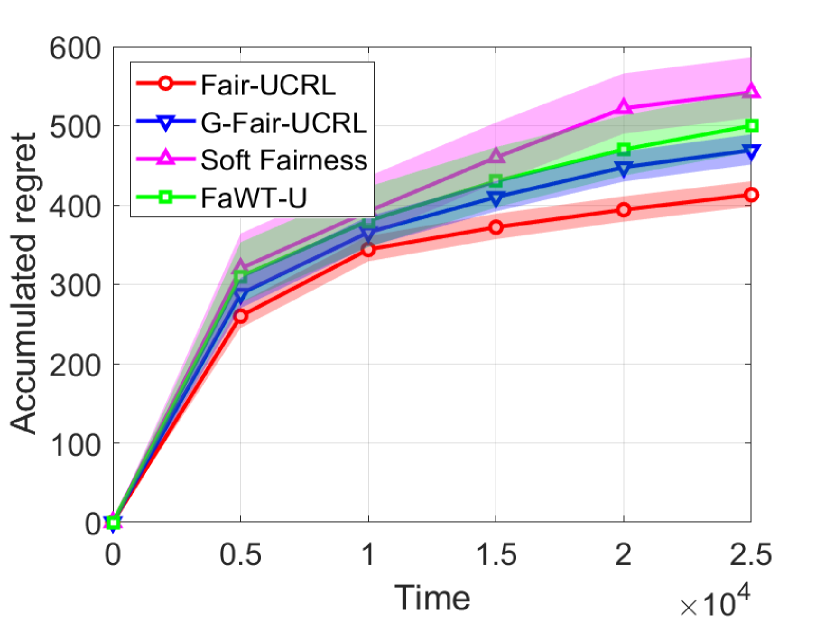
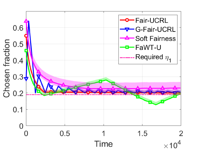
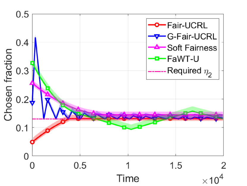
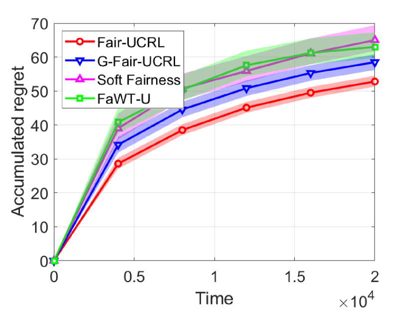
Reward Regret. The accumulated reward regrets are presented in Figureย 4, where we use Monte Carlo simulations with $1,000$ independent trials. Fair-UCRL achieves the lowest accumulated reward regret. More importantly, this is consistent with our theoretical analysis (see Theoremย 1), while neither FaWT-U nor Soft Fairness provides a finite-time analysis, i.e., nor provable regret bound guarantees.

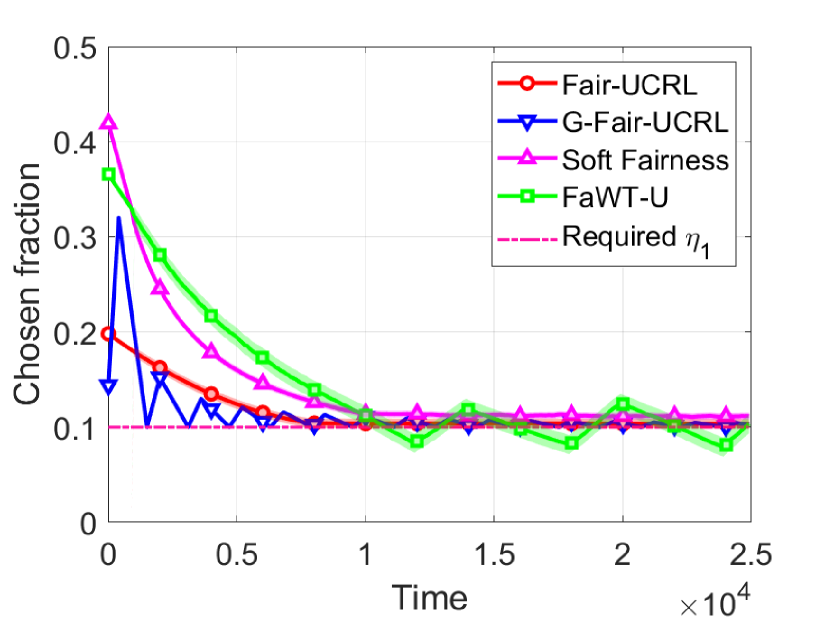
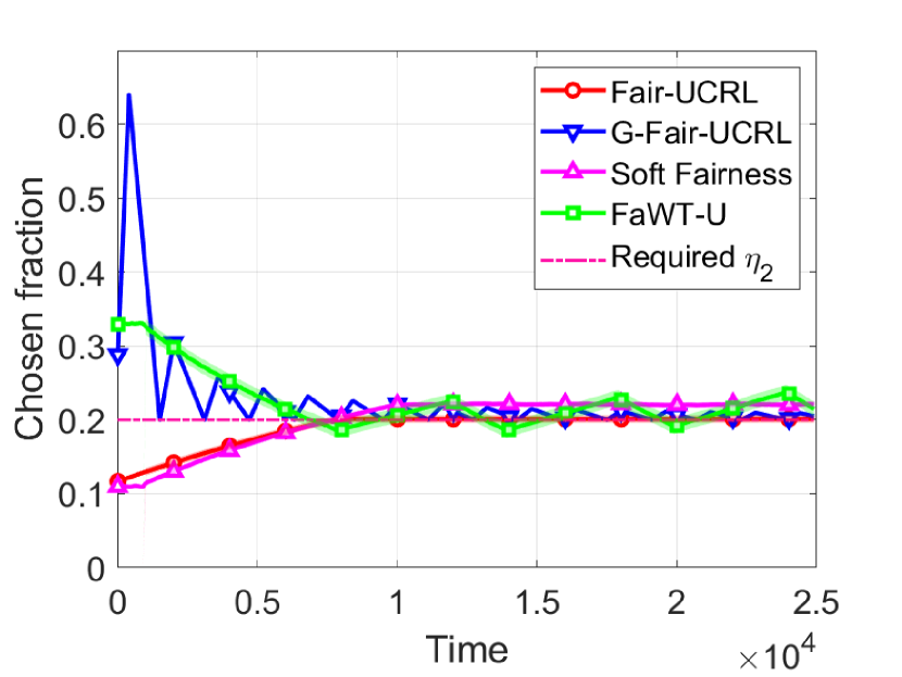
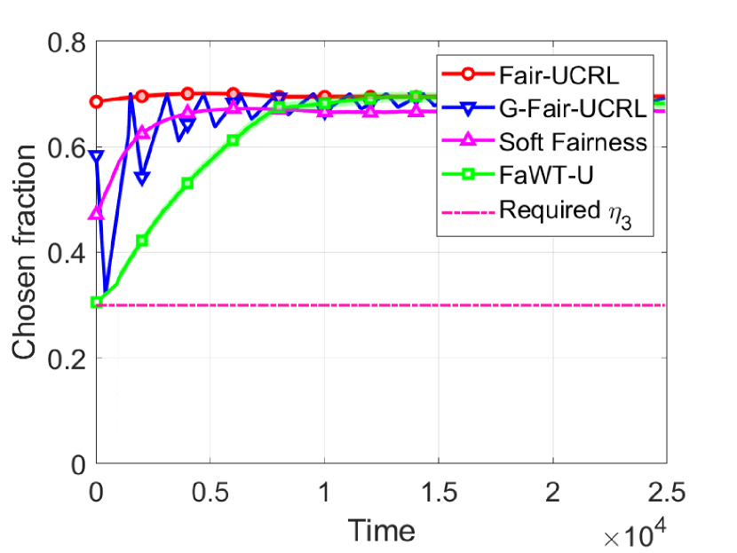
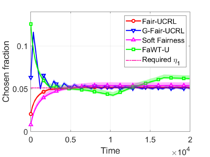
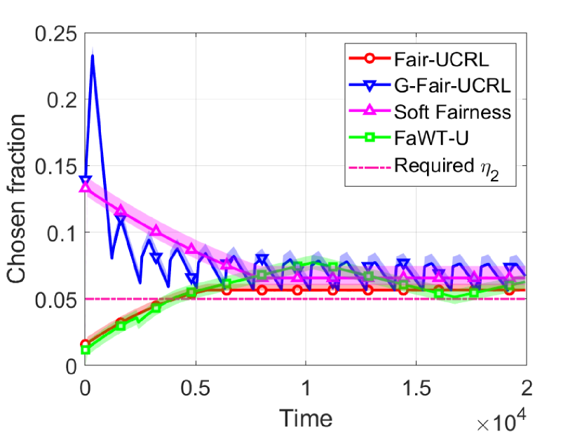
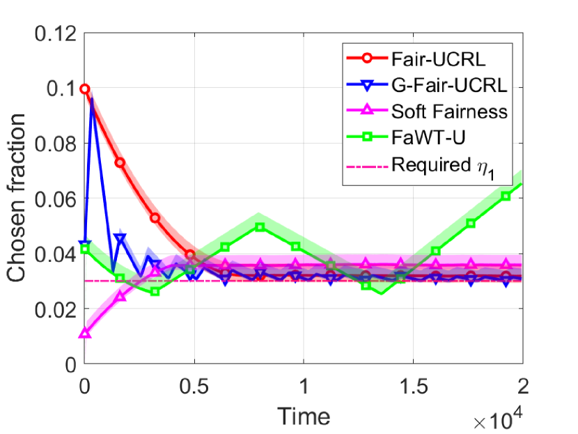
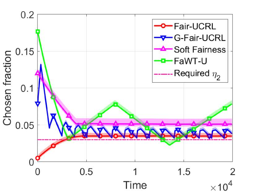
Fairness Constraint Violation. The activation fraction for each arm over time under different policies are presented in Figuresย 4,ย 4 andย 4, respectively. After a certain amount of time, the minimum activation fraction for each arm under Fair-UCRL is always satisfied, and a randomized initialization may cause short term fairness violation, for example, after 6,50065006,500 time steps for arm 2, even though the constraint needs to be satisfied on average. Similar observations hold for Soft Fairness, while for FaWT-U, fairness constraint violation repeatedly occurs over time for arm 1 and arm 2.

Refer to caption
(a) Reward regret.
Refer to caption
(b) Fairness constraint violation for arm 1.
Refer to caption
(c) Fairness constraint violation for arm 2.
Figure 6: PASCAL recognizing textual entailment task.
Refer to caption
(a) Reward regret.
Refer to caption
(b) Fairness constraint violation for arm 1.
Refer to caption
(c) Fairness constraint violation for arm 2.
Figure 7: Land mobile satellite system.

Continuous Positive Airway Pressure Therapy

We study the continuous positive airway pressure therapy (CPAP) as in Herlihy etย al. (2023); Li and Varakantham (2022b), which is a highly effective treatment when it is used consistently during the sleeping for adults with obstructive sleep apnea. Similar non-adherence to CPAP in patients hinders the effectiveness, we adapt the Markov model of CPAP adherence behavior (Kang etย al. 2013) to a two-state system with the clinical adherence criteria. Specifically, there are 3 states, representing low, intermediate and acceptable adherence levels. Patients are clustered into two groups, โ€œAdherenceโ€ and โ€œNon-Adherenceโ€. The first group has a higher probability of staying in a good adherence level. There are 20 arms/patients with 10 in each group. The transition matrix of arms in each group contains a randomized, small noise from the original data. The intervention, which is the action applied to each arm, results in a 5% to 50% increase in adherence level. The budget is B=5๐ต5B=5 and the fairness constraint is set to be a random number between [0.1, 0.7]. The objective is to maximize the total adherence level. The accumulated reward regret and the activation fraction for two randomly selected arms are presented in Figuresย 5,ย 5 andย 5, respectively. Again, we observe that Fair-UCRL achieves a much smaller reward regret and the fairness constraint is always satisfied after a certain amount of time.

PASCAL Recognizing Textual Entailment

We study the PASCAL recognizing textual entailment task as in Snow etย al. (2008). Workers are assigned with tasks that determine if hypothesis can be inferred from text. There are 10 workers. Due to lack of background information, a worker may not be able to correctly annotate a task. We assign a โ€œsuccessful annotation probabilityโ€ to each worker, which is based on the average success rate over 800 tasks in the dataset. Each worker is a MDP with state 1 (correctly annotated) and 0 (otherwise). The transition probability from state 0 to 1 with $a=1$ is the same as that of staying at state 1 with $a=1$, which is set as the successful annotation probability. Reward is $1$ if a selected worker successfully annotates the task, and 00 otherwise. At each time, 3 tasks are generated (i.e., $B=3$) and distributed to workers. Fairness constraints for all workers are set to be $\eta=0.05$. Again, both proposed algorithms outperform two baselines and maintain higher selection fraction as shown in Figuresย 6, ย 6 andย 6 for two randomly selected arms, respectively.

Land Mobile Satellite System

We study the land mobile satellite system problem as in Prieto-Cerdeira etย al. (2010), in which the land mobile satellite broadcasts a signal carrying multimedia services to handheld devices. There are 4 arms with different elevation angles ($40^{\circ},60^{\circ},70^{\circ},80^{\circ}$) of the antenna in urban area. Only two states (Good and bad) are considered and we leverage the same transition matrix as in Prieto-Cerdeira etย al. (2010). Similar, we use the average direct signal mean as the reward function. The budget is $B=2$. We apply the fairness constraint $\eta=0.03$ to all angles. Again, Fair-UCRL outperforms the considered baselines in reward regret (Figureย 7), while satisfies long term average fairness constraint (Figuresย 7 andย 7 for two randomly selected arms).

Acknowledgements

This work was supported in part by the National Science Foundation (NSF) grants 2148309 and 2315614, and was supported in part by funds from OUSD R&E, NIST, and industry partners as specified in the Resilient & Intelligent NextG Systems (RINGS) program. This work was also supported in part by the U.S. Army Research Office (ARO) grant W911NF-23-1-0072, and the U.S. Department of Energy (DOE) grant DE-EE0009341. Any opinions, findings, and conclusions or recommendations expressed in this material are those of the authors and do not necessarily reflect the views of the funding agencies.

References

  • Akbarzadeh and Mahajan (2022) Akbarzadeh, N.; and Mahajan, A. 2022. On learning Whittle index policy for restless bandits with scalable regret. arXiv preprint arXiv:2202.03463.
  • Altman (1999) Altman, E. 1999. Constrained Markov decision processes, volumeย 7. CRC Press.
  • Avrachenkov and Borkar (2022) Avrachenkov, K.ย E.; and Borkar, V.ย S. 2022. Whittle index based Q-learning for restless bandits with average reward. Automatica, 139: 110186.
  • Bhattacharya (2018) Bhattacharya, B. 2018. Restless bandits visiting villages: A preliminary study on distributing public health services. In Proceedings of the 1st ACM SIGCAS Conference on Computing and Sustainable Societies, 1โ€“8.
  • Biswas etย al. (2021) Biswas, A.; Aggarwal, G.; Varakantham, P.; and Tambe, M. 2021. Learn to intervene: An adaptive learning policy for restless bandits in application to preventive healthcare. In Proc. of IJCAI.
  • Biswas etย al. (2023) Biswas, A.; Killian, J.ย A.; Diaz, P.ย R.; Ghosh, S.; and Tambe, M. 2023. Fairness for Workers Who Pull the Arms: An Index Based Policy for Allocation of Restless Bandit Tasks. arXiv preprint arXiv:2303.00799.
  • Borkar, Ravikumar, and Saboo (2017) Borkar, V.ย S.; Ravikumar, K.; and Saboo, K. 2017. An index policy for dynamic pricing in cloud computing under price commitments. Applicationes Mathematicae, 44: 215โ€“245.
  • Chen, Jain, and Luo (2022) Chen, L.; Jain, R.; and Luo, H. 2022. Learning Infinite-Horizon Average-Reward Markov Decision Processes with Constraints. arXiv preprint arXiv:2202.00150.
  • Chen etย al. (2020) Chen, Y.; Cuellar, A.; Luo, H.; Modi, J.; Nemlekar, H.; and Nikolaidis, S. 2020. Fair contextual multi-armed bandits: Theory and experiments. In Conference on Uncertainty in Artificial Intelligence, 181โ€“190. PMLR.
  • Cinlar (1975) Cinlar, E. 1975. Introduction to stochastic processes Prentice-Hall. Englewood Cliffs, New Jersey (420p).
  • Cohen, Zhao, and Scaglione (2014) Cohen, K.; Zhao, Q.; and Scaglione, A. 2014. Restless multi-armed bandits under time-varying activation constraints for dynamic spectrum access. In 2014 48th Asilomar Conference on Signals, Systems and Computers, 1575โ€“1578. IEEE.
  • Dai etย al. (2011) Dai, W.; Gai, Y.; Krishnamachari, B.; and Zhao, Q. 2011. The Non-Bayesian Restless Multi-Armed Bandit: A Case of Near-Logarithmic Regret. In Proc. of IEEE ICASSP.
  • Dโ€™Amour etย al. (2020) Dโ€™Amour, A.; Srinivasan, H.; Atwood, J.; Baljekar, P.; Sculley, D.; and Halpern, Y. 2020. Fairness is not static: deeper understanding of long term fairness via simulation studies. In Proceedings of the 2020 Conference on Fairness, Accountability, and Transparency, 525โ€“534.
  • Duran and Verloop (2018) Duran, S.; and Verloop, I.ย M. 2018. Asymptotic optimal control of Markov-modulated restless bandits. Proceedings of the ACM on Measurement and Analysis of Computing Systems, 2(1): 1โ€“25.
  • Efroni, Mannor, and Pirotta (2020) Efroni, Y.; Mannor, S.; and Pirotta, M. 2020. Exploration-Exploitation in Constrained MDPs. arXiv preprint arXiv:2003.02189.
  • Fu etย al. (2019) Fu, J.; Nazarathy, Y.; Moka, S.; and Taylor, P.ย G. 2019. Towards q-learning the whittle index for restless bandits. In 2019 Australian & New Zealand Control Conference (ANZCC), 249โ€“254. IEEE.
  • Gast and Bruno (2010) Gast, N.; and Bruno, G. 2010. A mean field model of work stealing in large-scale systems. ACM SIGMETRICS Performance Evaluation Review, 38(1): 13โ€“24.
  • Glazebrook, Hodge, and Kirkbride (2011) Glazebrook, K.ย D.; Hodge, D.ย J.; and Kirkbride, C. 2011. General notions of indexability for queueing control and asset management. The Annals of Applied Probability, 21(3): 876โ€“907.
  • Herlihy etย al. (2023) Herlihy, C.; Prins, A.; Srinivasan, A.; and Dickerson, J.ย P. 2023. Planning to fairly allocate: Probabilistic fairness in the restless bandit setting. In Proceedings of the 29th ACM SIGKDD Conference on Knowledge Discovery and Data Mining, 732โ€“740.
  • Hodge and Glazebrook (2015) Hodge, D.ย J.; and Glazebrook, K.ย D. 2015. On the asymptotic optimality of greedy index heuristics for multi-action restless bandits. Advances in Applied Probability, 47(3): 652โ€“667.
  • Hu and Frazier (2017) Hu, W.; and Frazier, P. 2017. An Asymptotically Optimal Index Policy for Finite-Horizon Restless Bandits. arXiv preprint arXiv:1707.00205.
  • Jaksch, Ortner, and Auer (2010) Jaksch, T.; Ortner, R.; and Auer, P. 2010. Near-Optimal Regret Bounds for Reinforcement Learning. Journal of Machine Learning Research, 11(4).
  • Jung, Abeille, and Tewari (2019) Jung, Y.ย H.; Abeille, M.; and Tewari, A. 2019. Thompson Sampling in Non-Episodic Restless Bandits. arXiv preprint arXiv:1910.05654.
  • Jung and Tewari (2019) Jung, Y.ย H.; and Tewari, A. 2019. Regret Bounds for Thompson Sampling in Episodic Restless Bandit Problems. Proc. of NeurIPS.
  • Kalagarla, Jain, and Nuzzo (2021) Kalagarla, K.ย C.; Jain, R.; and Nuzzo, P. 2021. A Sample-Efficient Algorithm for Episodic Finite-Horizon MDP with Constraints. In Proc. of AAAI.
  • Kang etย al. (2013) Kang, Y.; Prabhu, V.ย V.; Sawyer, A.ย M.; and Griffin, P.ย M. 2013. Markov models for treatment adherence in obstructive sleep apnea. In IIE Annual Conference. Proceedings, 1592. Institute of Industrial and Systems Engineers (IISE).
  • Killian etย al. (2021) Killian, J.ย A.; Biswas, A.; Shah, S.; and Tambe, M. 2021. Q-Learning Lagrange Policies for Multi-Action Restless Bandits. In Proc. of ACM SIGKDD.
  • Killian, Perrault, and Tambe (2021) Killian, J.ย A.; Perrault, A.; and Tambe, M. 2021. Beyondโ€ To Act or Not to Actโ€: Fast Lagrangian Approaches to General Multi-Action Restless Bandits. In Proc.of AAMAS.
  • Larraรฑaga, Ayesta, and Verloop (2014) Larraรฑaga, M.; Ayesta, U.; and Verloop, I.ย M. 2014. Index Policies for A Multi-Class Queue with Convex Holding Cost and Abandonments. In Proc. of ACM Sigmetrics.
  • Lattimore and Szepesvรกri (2020) Lattimore, T.; and Szepesvรกri, C. 2020. Bandit Algorithms. Cambridge University Press.
  • Li and Varakantham (2022a) Li, D.; and Varakantham, P. 2022a. Efficient Resource Allocation with Fairness Constraints in Restless Multi-Armed Bandits. In Proc. of UAI.
  • Li and Varakantham (2022b) Li, D.; and Varakantham, P. 2022b. Towards Soft Fairness in Restless Multi-Armed Bandits. arXiv preprint arXiv:2207.13343.
  • Li, Liu, and Ji (2019) Li, F.; Liu, J.; and Ji, B. 2019. Combinatorial sleeping bandits with fairness constraints. IEEE Transactions on Network Science and Engineering, 7(3): 1799โ€“1813.
  • Liu, Liu, and Zhao (2011) Liu, H.; Liu, K.; and Zhao, Q. 2011. Logarithmic Weak Regret of Non-Bayesian Restless Multi-Armed Bandit. In Proc of IEEE ICASSP.
  • Liu, Liu, and Zhao (2012) Liu, H.; Liu, K.; and Zhao, Q. 2012. Learning in A Changing World: Restless Multi-Armed Bandit with Unknown Dynamics. IEEE Transactions on Information Theory, 59(3): 1902โ€“1916.
  • Mate, Perrault, and Tambe (2021) Mate, A.; Perrault, A.; and Tambe, M. 2021. Risk-Aware Interventions in Public Health: Planning with Restless Multi-Armed Bandits. In Proc.of AAMAS.
  • Maurer and Pontil (2009) Maurer, A.; and Pontil, M. 2009. Empirical Bernstein Bounds and Sample Variance Penalization. arXiv preprint arXiv:0907.3740.
  • Mitrophanov (2005) Mitrophanov, A.ย Y. 2005. Sensitivity and convergence of uniformly ergodic Markov chains. Journal of Applied Probability, 42(4): 1003โ€“1014.
  • Nakhleh etย al. (2021) Nakhleh, K.; Ganji, S.; Hsieh, P.-C.; Hou, I.; Shakkottai, S.; etย al. 2021. NeurWIN: Neural Whittle Index Network For Restless Bandits Via Deep RL. Proc. of NeurIPS.
  • Nakhleh, Hou etย al. (2022) Nakhleh, K.; Hou, I.; etย al. 2022. DeepTOP: Deep Threshold-Optimal Policy for MDPs and RMABs. In Proc. of NeurIPS.
  • Niรฑo-Mora (2007) Niรฑo-Mora, J. 2007. Dynamic Priority Allocation via Restless Bandit Marginal Productivity Indices. Top, 15(2): 161โ€“198.
  • Ortner etย al. (2012) Ortner, R.; Ryabko, D.; Auer, P.; and Munos, R. 2012. Regret Bounds for Restless Markov Bandits. In Proc. of Algorithmic Learning Theory.
  • Papadimitriou and Tsitsiklis (1994) Papadimitriou, C.ย H.; and Tsitsiklis, J.ย N. 1994. The Complexity of Optimal Queueing Network Control. In Proc. of IEEE Conference on Structure in Complexity Theory.
  • Prieto-Cerdeira etย al. (2010) Prieto-Cerdeira, R.; Perez-Fontan, F.; Burzigotti, P.; Bolea-Alamaรฑac, A.; and Sanchez-Lago, I. 2010. Versatile two-state land mobile satellite channel model with first application to DVB-SH analysis. International Journal of Satellite Communications and Networking, 28(5-6): 291โ€“315.
  • Puterman (1994) Puterman, M.ย L. 1994. Markov Decision Processes: Discrete Stochastic Dynamic Programming. John Wiley & Sons.
  • Sheng, Liu, and Saigal (2014) Sheng, S.-P.; Liu, M.; and Saigal, R. 2014. Data-Driven Channel Modeling Using Spectrum Measurement. IEEE Transactions on Mobile Computing, 14(9): 1794โ€“1805.
  • Singh, Gupta, and Shroff (2020) Singh, R.; Gupta, A.; and Shroff, N.ย B. 2020. Learning in Markov decision processes under constraints. arXiv preprint arXiv:2002.12435.
  • Snow etย al. (2008) Snow, R.; Oโ€™connor, B.; Jurafsky, D.; and Ng, A.ย Y. 2008. Cheap and fastโ€“but is it good? Evaluating non-expert annotations for natural language tasks. In Proceedings of the 2008 conference on empirical methods in natural language processing, 254โ€“263.
  • Tekin and Liu (2011) Tekin, C.; and Liu, M. 2011. Adaptive Learning of Uncontrolled Restless Bandits with Logarithmic Regret. In Proc. of Allerton.
  • Tekin and Liu (2012) Tekin, C.; and Liu, M. 2012. Online Learning of Rested and Restless Bandits. IEEE Transactions on Information Theory, 58(8): 5588โ€“5611.
  • Verloop (2016) Verloop, I.ย M. 2016. Asymptotically Optimal Priority Policies for Indexable and Nonindexable Restless Bandits. The Annals of Applied Probability, 26(4): 1947โ€“1995.
  • Wang, Huang, and Lui (2020) Wang, S.; Huang, L.; and Lui, J. 2020. Restless-UCB, an Efficient and Low-complexity Algorithm for Online Restless Bandits. In Proc. of NeurIPS.
  • Weber and Weiss (1990) Weber, R.ย R.; and Weiss, G. 1990. On An Index Policy for Restless Bandits. Journal of Applied Probability, 637โ€“648.
  • Whittle (1988) Whittle, P. 1988. Restless Bandits: Activity Allocation in A Changing World. Journal of Applied Probability, 287โ€“298.
  • Xiong and Li (2023) Xiong, G.; and Li, J. 2023. Finite-Time Analysis of Whittle Index based Q-Learning for Restless Multi-Armed Bandits with Neural Network Function Approximation. In Proc. of NeurIPS.
  • Xiong, Li, and Singh (2022) Xiong, G.; Li, J.; and Singh, R. 2022. Reinforcement Learning Augmented Asymptotically Optimal Index Policy for Finite-Horizon Restless Bandits. In Proc. of AAAI.
  • Xiong, Wang, and Li (2022) Xiong, G.; Wang, S.; and Li, J. 2022. Learning Infinite-Horizon Average-Reward Restless Multi-Action Bandits via Index Awareness. In Proc. of NeurIPS.
  • Xiong etย al. (2022) Xiong, G.; Wang, S.; Yan, G.; and Li, J. 2022. Reinforcement Learning for Dynamic Dimensioning of Cloud Caches: A Restless Bandit Approach. In Proc. of IEEE INFOCOM.
  • Yin etย al. (2023) Yin, T.; Raab, R.; Liu, M.; and Liu, Y. 2023. Long-Term Fairness with Unknown Dynamics. arXiv preprint arXiv:2304.09362.
  • Zayas-Cabรกn, Jasin, and Wang (2019) Zayas-Cabรกn, G.; Jasin, S.; and Wang, G. 2019. An Asymptotically Optimal Heuristic for General Nonstationary Finite-Horizon Restless Multi-Armed, Multi-Action Bandits. Advances in Applied Probability, 51(3): 745โ€“772.
  • Zhang and Frazier (2021) Zhang, X.; and Frazier, P.ย I. 2021. Restless Bandits with Many Arms: Beating the Central Limit Theorem. arXiv preprint arXiv:2107.11911.
  • Zou etย al. (2021) Zou, Y.; Kim, K.ย T.; Lin, X.; and Chiang, M. 2021. Minimizing Age-of-Information in Heterogeneous Multi-Channel Systems: A New Partial-Index Approach. In Proc. of ACM MobiHoc.

Appendix A Related Work

Offline RMAB. The RMAB was first introduced in (Whittle 1988), which is known to be computationally intractable and is in general PSPACE hard (Papadimitriou and Tsitsiklis 1994). The state-of-the-art approach to RMAB is the Whittle index policy, which is provably asymptotically optimal (Weber and Weiss 1990). However, Whittle index is well-defined only when the indexability condition is satisfied, which is in general hard to verify. Furthermore, even when an arm is indexable, finding its Whittle index can still be intractable (Niรฑo-Mora 2007). As a result, Whittle indices of many practical problems remain unknown. Exacerbating these limitations is the fact that these Whittle-like index policies fail to provide any guarantee on how activation is distributed among arms. To address fairness concerns, there are recent efforts on imposing fairness constraints in RMAB, e.g., Li and Varakantham (2022a); Herlihy etย al. (2023). However, they either considered the finite-horizon or infinite-horizon discounted reward setting, and hence cannot be directly applied to the more challenging infinite-horizon average-reward setting with long-term fairness constraints considered in this paper. In addition, there is no rigorous finite-time performance analysis in terms of regret in Li and Varakantham (2022a); Herlihy etย al. (2023). The probabilistic fairness guarantees in Herlihy etย al. (2023) are restricted to a 2-state MDP and cannot be easily extended to a general MDP as considered in this paper.

Online RMAB. Since the underlying MDPs associated with each arm in RMAB are unknown in practice, it is important to examine RMAB from a learning perspective, e.g., (Dai etย al. 2011; Tekin and Liu 2011; Liu, Liu, and Zhao 2011, 2012; Tekin and Liu 2012; Ortner etย al. 2012; Jung and Tewari 2019; Jung, Abeille, and Tewari 2019; Wang, Huang, and Lui 2020). However, these methods either leveraged a heuristic policy and may not perform close to the offline optimum, or are computationally expensive. Recently, low-complexity RL algorithms have been developed for RMAB, e.g., Fu etย al. (2019); Avrachenkov and Borkar (2022); Biswas etย al. (2021); Killian etย al. (2021); Wang, Huang, and Lui (2020); Xiong, Li, and Singh (2022); Xiong, Wang, and Li (2022); Xiong etย al. (2022); Nakhleh etย al. (2021); Nakhleh, Hou etย al. (2022). However, none of these studies are applicable to RMAB-F, where the DM not only needs to maximize the long-term reward under the instantaneous activation constraint as in RMAB, but ensures that a long-term fairness constraint is satisfied for each arm. Our RL algorithm with rigorous regret analysis on both the reward and the fairness violation further differentiate our work.

Appendix B The Fair-UCRL Algorithm

Algorithm Overview. Fair-UCRL proceeds in episodes as summarized in Algorithmย 1. Let $\tau_{k}$ be the start time of episode $k$. Each episode consists of two phases: (i) Optimistic planning: At the beginning of each episode (line 4 in Algorithmย 1), Fair-UCRL constructs a confidence ball that contains a set of plausible MDPs (Jaksch, Ortner, and Auer 2010) for each arm $\forall n\in\mathcal{N}$. To obtain an optimistic estimate of the true transition kernels and rewards, Fair-UCRL solves an optimistic planning problem with parameters chosen from the constructed confidence ball. Since the online RMAB-F is computationally intractable, we first relax the instantaneous activation constraint to a โ€œlong-term activation constraintโ€, from which we obtain a linear programming (LP) where decision variables are the occupancy measures (Altman 1999) corresponding to the process associated with $N$ arms. We refer to the planning problem as an extended LP (line 5 in Algorithmย 1), which is described in details below. (ii) Policy execution: Unfortunately, the solutions to this extended LP is not always feasible to the online RMAB-F, which requires the instantaneous activation constraint to be satisfied at each decision epoch, rather than in the average sense as in the extended LP. To address this challenge, Fair-UCRL constructs a so-called FairRMAB index policy on top of the solutions to the extended LP, which is executed during the policy execution phase of each episode (lines 7-8 in Algorithmย 1).

Optimistic Planning.

Fair-UCRL maintains two counts for each arm $n$. Let Cnkโˆ’1โ€‹(s,a)superscriptsubscript๐ถ๐‘›๐‘˜1๐‘ ๐‘ŽC_{n}^{k-1}(s,a) be the number of visits to state-action pairs (s,a)๐‘ ๐‘Ž(s,a) until $\tau_{k}$, and Cnkโˆ’1โ€‹(s,a,sโ€ฒ)superscriptsubscript๐ถ๐‘›๐‘˜1๐‘ ๐‘Žsuperscript๐‘ โ€ฒC_{n}^{k-1}(s,a,s^{\prime}) be the number of transitions from s๐‘ s to sโ€ฒsuperscript๐‘ โ€ฒs^{\prime} under action $a$ until $\tau_{k}$. At the end of episode $k$, Fair-UCRL updates these counts as Cnkโ€‹(s,a)=Cnkโˆ’1โ€‹(s,a)+โˆ‘h=1H๐Ÿ™โ€‹(snkโ€‹(h)=s,ankโ€‹(h)=a),superscriptsubscript๐ถ๐‘›๐‘˜๐‘ ๐‘Žsuperscriptsubscript๐ถ๐‘›๐‘˜1๐‘ ๐‘Žsuperscriptsubscriptโ„Ž1๐ป1formulae-sequencesuperscriptsubscript๐‘ ๐‘›๐‘˜โ„Ž๐‘ superscriptsubscript๐‘Ž๐‘›๐‘˜โ„Ž๐‘ŽC_{n}^{k}(s,a)=C_{n}^{k-1}(s,a)+\sum_{h=1}^{H}\mathds{1}(s_{n}^{k}(h)=s,a_{n}^{k}(h)=a), and $C_{n}^{k}(s,a,s^{\prime})=C_{n}^{k-1}(s,a,s^{\prime})+\sum_{h=1}^{H}\mathds{1}(s_{n}^{k}(h+1)=s^{\prime}|s_{n}^{k}(h)=s,a_{n}^{k}(h)=a)$, โˆ€(s,a)โˆˆ๐’ฎร—๐’œfor-all๐‘ ๐‘Ž๐’ฎ๐’œ\forall(s,a)\in\mathcal{S}\times\mathcal{A} and โˆ€(s,a,sโ€ฒ)โˆˆ๐’ฎร—๐’œร—๐’ฎfor-all๐‘ ๐‘Žsuperscript๐‘ โ€ฒ๐’ฎ๐’œ๐’ฎ\forall(s,a,s^{\prime})\in\mathcal{S}\times\mathcal{A}\times\mathcal{S} for each arm $n$, where snkโ€‹(h)superscriptsubscript๐‘ ๐‘›๐‘˜โ„Žs_{n}^{k}(h) is the state of arm $n$ at the $h$-th time frame in episode $k$. Then Fair-UCRL estimates the true transition kernel and the true reward function by the corresponding empirical averages as:

P^nkโ€‹(sโ€ฒ|s,a)=Cnkโˆ’1โ€‹(s,a,sโ€ฒ)maxโก{Cnkโˆ’1โ€‹(s,a),1},superscriptsubscript^๐‘ƒ๐‘›๐‘˜conditionalsuperscript๐‘ โ€ฒ๐‘ ๐‘Žsuperscriptsubscript๐ถ๐‘›๐‘˜1๐‘ ๐‘Žsuperscript๐‘ โ€ฒsuperscriptsubscript๐ถ๐‘›๐‘˜1๐‘ ๐‘Ž1\displaystyle\hat{P}_{n}^{k}(s^{\prime}|s,a)\!=\!\frac{C_{n}^{k-1}(s,a,s^{\prime})}{\max\{C_{n}^{k-1}(s,a),1\}}, (9)
r^nkโ€‹(s,a)=โˆ‘l=1kโˆ’1โˆ‘h=1Hrnlโ€‹(s,a)โ€‹๐Ÿ™โ€‹(snlโ€‹(h)=s,anlโ€‹(h)=a)maxโก{Cnkโˆ’1โ€‹(s,a),1}.superscriptsubscript^๐‘Ÿ๐‘›๐‘˜๐‘ ๐‘Žsuperscriptsubscript๐‘™1๐‘˜1superscriptsubscriptโ„Ž1๐ปsuperscriptsubscript๐‘Ÿ๐‘›๐‘™๐‘ ๐‘Ž1formulae-sequencesuperscriptsubscript๐‘ ๐‘›๐‘™โ„Ž๐‘ superscriptsubscript๐‘Ž๐‘›๐‘™โ„Ž๐‘Žsuperscriptsubscript๐ถ๐‘›๐‘˜1๐‘ ๐‘Ž1\displaystyle\hat{r}_{n}^{k}(s,a)\!=\!\frac{\sum\limits_{l=1}^{k-1}\sum\limits_{h=1}^{H}r_{n}^{l}(s,a)\mathds{1}(s_{n}^{l}(h)=s,a_{n}^{l}(h)=a)}{\max\{C_{n}^{k-1}(s,a),1\}}. (10)

Fair-UCRL further defines confidence intervals for transition probabilities and rewards so that true transition probabilities and true rewards lie in them with high probabilities, respectively. Formally, for โˆ€(s,a)โˆˆ๐’ฎร—๐’œfor-all๐‘ ๐‘Ž๐’ฎ๐’œ\forall(s,a)\in\mathcal{S}\times\mathcal{A}, we define

๐’ซnkโ€‹(s,a)superscriptsubscript๐’ซ๐‘›๐‘˜๐‘ ๐‘Ž\displaystyle\mathcal{P}_{n}^{k}(s,a) $\displaystyle:=\{\tilde{P}_{n}^{k}(s^{\prime}|s,a),\forall s^{\prime}:$
$\displaystyle|\tilde{P}_{n}^{k}(s^{\prime}|s,a)-\hat{P}_{n}^{k}(s^{\prime}|s,a)|\leq\delta_{n}^{k}(s,a)\},$ (11)
โ„›nkโ€‹(s,a)superscriptsubscriptโ„›๐‘›๐‘˜๐‘ ๐‘Ž\displaystyle\mathcal{R}_{n}^{k}(s,a) $\displaystyle:=\{\tilde{r}_{n}^{k}(s,a):$
$\displaystyle|\tilde{r}_{n}^{k}(s,a)-\hat{r}_{n}^{k}(s,a)|\leq\delta_{n}^{k}(s,a)\},$ (12)

where the size of the confidence intervals ฮดnkโ€‹(s,a)superscriptsubscript๐›ฟ๐‘›๐‘˜๐‘ ๐‘Ž\delta_{n}^{k}(s,a) is built according to the Hoeffding inequality (Maurer and Pontil 2009) for $\epsilon\in(0,1)$ as

ฮดnkโ€‹(s,a)=12โ€‹Cnkโˆ’1โ€‹(s,a)โ€‹logโก(Sโ€‹Aโ€‹Nโ€‹(kโˆ’1)โ€‹Hฯต).superscriptsubscript๐›ฟ๐‘›๐‘˜๐‘ ๐‘Ž12superscriptsubscript๐ถ๐‘›๐‘˜1๐‘ ๐‘Ž๐‘†๐ด๐‘๐‘˜1๐ปitalic-ฯต\displaystyle\delta_{n}^{k}(s,a)=\sqrt{\frac{1}{2C_{n}^{k-1}(s,a)}\log\bigg{(}\frac{SAN(k-1)H}{\epsilon}\bigg{)}}. (13)

To this end, we define a set of plausible MDPs associated with the confidence intervals in episode $k$:

$\displaystyle\mathcal{M}^{k}$ $\displaystyle=\big{\{}M_{n}^{k}=(\mathcal{S},\mathcal{A},\tilde{P}_{n}^{k},\tilde{r}_{n}^{k}):|\tilde{P}_{n}^{k}(s^{\prime}|s,a)-\hat{P}_{n}^{k}(s^{\prime}|s,a)|$
$\displaystyle\leq\delta_{n}^{k}(s,a),\tilde{r}_{n}^{k}(s,a)=\hat{r}_{n}^{k}(s,a)+\delta_{n}^{k}(s,a)\big{\}}.$ (14)

Fair-UCRL computes a policy $\pi^{k,*}$ by performing optimistic planning. In other words, in each episode $k,$ given the set of plausible MDPsย (B), Fair-UCRL selects an optimistic MDP $M_{n}^{k},\forall n$ and an optimistic policy with respect to RMAB-F ($\tilde{P}_{n}^{k},\tilde{r}_{n}^{k},\forall n$), which is similar to the offline RMAB-F ($P_{n},r_{n},\forall n$) inย (1)-(3) by replacing transition and reward functions with $\tilde{P}_{n}^{k}(\cdot|\cdot,\cdot)$ and $\tilde{r}_{n}^{k}(\cdot,\cdot)$, โˆ€s,a,sโ€ฒ,n,kfor-all๐‘ ๐‘Žsuperscript๐‘ โ€ฒ๐‘›๐‘˜\forall s,a,s^{\prime},n,k, respectively, in the confidence intervalsย (11),(12) due to the fact that the corresponding true values are not available.

As aforementioned, it is well known that solving RMAB-F ($\tilde{P}_{n}^{k},\tilde{r}_{n}^{k},\forall n$) is intractable even in the offline setting (Whittle 1988). To address this challenge, we first relax the instantaneous activation constraint so as to achieve a โ€œlong-term activation constraintโ€, i.e., the activation. For simplicity, we call RMAB-F ($\tilde{P}_{n}^{k},\tilde{r}_{n}^{k},\forall n$) with the long-term activation constraint as โ€œthe relaxed RMAB-F ($\tilde{P}_{n}^{k},\tilde{r}_{n}^{k},\forall n$)โ€. It turns out that this relaxed RMAB-F ($\tilde{P}_{n}^{k},\tilde{r}_{n}^{k},\forall n$) can be equivalently transformed into a linear programming (LP) via replacing all random variables in the relaxed RMAB-F ($\tilde{P}_{n}^{k},\tilde{r}_{n}^{k},\forall n$) with the occupancy measure corresponding to each arm $n$ (Altman 1999).

Extended LP. We cannot solve this LP since we have no knowledge about true transition kernels and rewards. Thus we further rewrite it as an extended LP by leveraging state-action-state occupancy measure znkโ€‹(s,a,sโ€ฒ)superscriptsubscript๐‘ง๐‘›๐‘˜๐‘ ๐‘Žsuperscript๐‘ โ€ฒz_{n}^{k}(s,a,s^{\prime}) to express confidence intervals of transition probabilities: given a policy $\pi$ and transition functions $\tilde{P}_{n}^{k},$ the occupancy measure znkโ€‹(s,a,sโ€ฒ)superscriptsubscript๐‘ง๐‘›๐‘˜๐‘ ๐‘Žsuperscript๐‘ โ€ฒz_{n}^{k}(s,a,s^{\prime}) induced by $\pi$ and $\tilde{P}_{n}^{k}$ is that โˆ€n,s,sโ€ฒ,a,kfor-all๐‘›๐‘ superscript๐‘ โ€ฒ๐‘Ž๐‘˜\forall n,s,s^{\prime},a,k: znkโ€‹(s,a,sโ€ฒ):=limHโ†’โˆž1Hโ€‹๐”ผฯ€โ€‹[โˆ‘h=1Hโˆ’1๐Ÿ™โ€‹(snโ€‹(h)=s,anโ€‹(h)=a,snโ€‹(h+1)=sโ€ฒ)].assignsuperscriptsubscript๐‘ง๐‘›๐‘˜๐‘ ๐‘Žsuperscript๐‘ โ€ฒsubscriptโ†’๐ป1๐ปsubscript๐”ผ๐œ‹delimited-[]superscriptsubscriptโ„Ž1๐ป11formulae-sequencesubscript๐‘ ๐‘›โ„Ž๐‘ formulae-sequencesubscript๐‘Ž๐‘›โ„Ž๐‘Žsubscript๐‘ ๐‘›โ„Ž1superscript๐‘ โ€ฒz_{n}^{k}(s,a,s^{\prime})\!:=\!\lim_{H\rightarrow\infty}\frac{1}{H}\mathbb{E}_{\pi}[\sum_{h=1}^{H-1}\mathds{1}(s_{n}(h)\!=\!s,a_{n}(h)\!=\!a,s_{n}(h+1)=s^{\prime})].

The extended LP over zk:={znkโ€‹(s,a,sโ€ฒ),โˆ€nโˆˆ๐’ฉ}assignsuperscript๐‘ง๐‘˜superscriptsubscript๐‘ง๐‘›๐‘˜๐‘ ๐‘Žsuperscript๐‘ โ€ฒfor-all๐‘›๐’ฉz^{k}:=\{z_{n}^{k}(s,a,s^{\prime}),\forall n\in\mathcal{N}\} is then given as $\textbf{ELP}(\mathcal{M}^{k},z^{k}):$

$\displaystyle\min_{z^{k}}$ โˆ‘n=1Nโˆ‘(s,a,sโ€ฒ)znkโ€‹(s,a,sโ€ฒ)โ€‹r~nkโ€‹(s,a)superscriptsubscript๐‘›1๐‘subscript๐‘ ๐‘Žsuperscript๐‘ โ€ฒsuperscriptsubscript๐‘ง๐‘›๐‘˜๐‘ ๐‘Žsuperscript๐‘ โ€ฒsuperscriptsubscript~๐‘Ÿ๐‘›๐‘˜๐‘ ๐‘Ž\displaystyle~{}\sum_{n=1}^{N}\sum_{(s,a,s^{\prime})}z_{n}^{k}(s,a,s^{\prime})\tilde{r}_{n}^{k}(s,a) (15)
s.t. โˆ‘n=1Nโˆ‘sโˆˆ๐’ฎโˆ‘sโ€ฒโˆˆ๐’ฎznkโ€‹(s,1,sโ€ฒ)โ‰คB,superscriptsubscript๐‘›1๐‘subscript๐‘ ๐’ฎsubscriptsuperscript๐‘ โ€ฒ๐’ฎsuperscriptsubscript๐‘ง๐‘›๐‘˜๐‘ 1superscript๐‘ โ€ฒ๐ต\displaystyle~{}\sum_{n=1}^{N}\sum_{s\in\mathcal{S}}\sum_{s^{\prime}\in\mathcal{S}}z_{n}^{k}(s,1,s^{\prime})\leq B, (16)
โˆ‘sโˆˆ๐’ฎโˆ‘sโ€ฒโˆˆ๐’ฎznkโ€‹(s,1,sโ€ฒ)โ‰ฅฮทn,โˆ€nโˆˆ๐’ฉ,formulae-sequencesubscript๐‘ ๐’ฎsubscriptsuperscript๐‘ โ€ฒ๐’ฎsuperscriptsubscript๐‘ง๐‘›๐‘˜๐‘ 1superscript๐‘ โ€ฒsubscript๐œ‚๐‘›for-all๐‘›๐’ฉ\displaystyle~{}\sum_{s\in\mathcal{S}}\sum_{s^{\prime}\in\mathcal{S}}z_{n}^{k}(s,1,s^{\prime})\geq\eta_{n},~{}\forall n\in\mathcal{N}, (17)
โˆ‘aโˆˆ๐’œโˆ‘sโ€ฒโˆˆ๐’ฎznkโ€‹(s,a,sโ€ฒ)=โˆ‘sโ€ฒโˆˆ๐’ฎโˆ‘aโ€ฒโˆˆ๐’œznkโ€‹(sโ€ฒ,aโ€ฒ,s),subscript๐‘Ž๐’œsubscriptsuperscript๐‘ โ€ฒ๐’ฎsuperscriptsubscript๐‘ง๐‘›๐‘˜๐‘ ๐‘Žsuperscript๐‘ โ€ฒsubscriptsuperscript๐‘ โ€ฒ๐’ฎsubscriptsuperscript๐‘Žโ€ฒ๐’œsuperscriptsubscript๐‘ง๐‘›๐‘˜superscript๐‘ โ€ฒsuperscript๐‘Žโ€ฒ๐‘ \displaystyle~{}\sum_{a\in\mathcal{A}}\sum_{s^{\prime}\in\mathcal{S}}z_{n}^{k}(s,a,s^{\prime})=\sum_{s^{\prime}\in\mathcal{S}}\sum_{a^{\prime}\in\mathcal{A}}z_{n}^{k}(s^{\prime},a^{\prime},s), (18)
โˆ‘sโˆˆ๐’ฎโˆ‘aโˆˆ๐’œโˆ‘sโ€ฒโˆˆ๐’ฎznkโ€‹(s,a,sโ€ฒ)=1,โˆ€nโˆˆ๐’ฉ,formulae-sequencesubscript๐‘ ๐’ฎsubscript๐‘Ž๐’œsubscriptsuperscript๐‘ โ€ฒ๐’ฎsuperscriptsubscript๐‘ง๐‘›๐‘˜๐‘ ๐‘Žsuperscript๐‘ โ€ฒ1for-all๐‘›๐’ฉ\displaystyle~{}\sum_{s\in\mathcal{S}}\sum_{a\in\mathcal{A}}\sum_{s^{\prime}\in\mathcal{S}}z_{n}^{k}(s,a,s^{\prime})=1,~{}\forall n\in\mathcal{N}, (19)
znkโ€‹(s,a,sโ€ฒ)โˆ‘yznkโ€‹(s,a,y)โˆ’(P^nkโ€‹(sโ€ฒ|s,a)+ฮดnkโ€‹(s,a))โ‰ค0,superscriptsubscript๐‘ง๐‘›๐‘˜๐‘ ๐‘Žsuperscript๐‘ โ€ฒsubscript๐‘ฆsuperscriptsubscript๐‘ง๐‘›๐‘˜๐‘ ๐‘Ž๐‘ฆsuperscriptsubscript^๐‘ƒ๐‘›๐‘˜conditionalsuperscript๐‘ โ€ฒ๐‘ ๐‘Žsuperscriptsubscript๐›ฟ๐‘›๐‘˜๐‘ ๐‘Ž0\displaystyle~{}\frac{z_{n}^{k}(s,a,s^{\prime})}{\sum_{y}z_{n}^{k}(s,a,y)}\!-\!(\hat{P}_{n}^{k}(s^{\prime}|s,a)\!+\!\delta_{n}^{k}(s,a))\leq 0, (20)
โˆ’znkโ€‹(s,a,sโ€ฒ)โˆ‘yznkโ€‹(s,a,y)+(P^nkโ€‹(sโ€ฒ|s,a)โˆ’ฮดnkโ€‹(s,a))โ‰ค0,superscriptsubscript๐‘ง๐‘›๐‘˜๐‘ ๐‘Žsuperscript๐‘ โ€ฒsubscript๐‘ฆsuperscriptsubscript๐‘ง๐‘›๐‘˜๐‘ ๐‘Ž๐‘ฆsuperscriptsubscript^๐‘ƒ๐‘›๐‘˜conditionalsuperscript๐‘ โ€ฒ๐‘ ๐‘Žsuperscriptsubscript๐›ฟ๐‘›๐‘˜๐‘ ๐‘Ž0\displaystyle\!-\!\frac{z_{n}^{k}(s,a,s^{\prime})}{\sum_{y}z_{n}^{k}(s,a,y)}\!+\!(\hat{P}_{n}^{k}(s^{\prime}|s,a)\!-\!\delta_{n}^{k}(s,a))\leq 0, (21)

where constraintsย (16)-(17) are restatements of โ€œlong-term activation constraintโ€ and โ€œlong-term fairness constraintโ€, respectively; constraintย (18) represents the fluid transition of occupancy measure; and constraintย (19) holds since the occupancy measure is a probability measure; and the last two constraints enforce that transition probabilities are inside of the confidence ballย (B). Denote the optimal solution to the extended LP as $z^{k,*}=\{z_{n}^{k,*},\forall n\in\mathcal{N}\}$.

Policy Execution.

One challenge for online RMAB-F ($\tilde{P}_{n}^{k},\tilde{r}_{n}^{k},\forall n$) is that the instantaneous activation constraint must be satisfied at each decision epoch, rather than in the average sense as in the extended LPย (15)-(21). As a result, the solution to the above extended LP is not always feasible to the online RMAB-F ($\tilde{P}_{n}^{k},\tilde{r}_{n}^{k},\forall n$). Inspired by (Xiong, Wang, and Li 2022), we construct an index policy, which is feasible for the online RMAB-F ($\tilde{P}_{n}^{k},\tilde{r}_{n}^{k},\forall n$). Specifically, we derive our index policy on top of the optimal solution $z^{k,*}=\{z_{n}^{k,*},\forall n\in\mathcal{N}\}$. Since $\mathcal{A}=\{0,1\}$, i.e, an arm can be either active or passive at time $t$, we define the index assigned to arm $n$ in state snโ€‹(t)=ssubscript๐‘ ๐‘›๐‘ก๐‘ s_{n}(t)=s at time $t$ to be as

ฯ‰nk,โˆ—โ€‹(s):=โˆ‘sโ€ฒznk,โˆ—โ€‹(s,1,sโ€ฒ)โˆ‘a,sโ€ฒznk,โˆ—โ€‹(s,a,sโ€ฒ),โˆ€nโˆˆ๐’ฉ.formulae-sequenceassignsuperscriptsubscript๐œ”๐‘›๐‘˜๐‘ subscriptsuperscript๐‘ โ€ฒsuperscriptsubscript๐‘ง๐‘›๐‘˜๐‘ 1superscript๐‘ โ€ฒsubscript๐‘Žsuperscript๐‘ โ€ฒsuperscriptsubscript๐‘ง๐‘›๐‘˜๐‘ ๐‘Žsuperscript๐‘ โ€ฒfor-all๐‘›๐’ฉ\displaystyle\omega_{n}^{k,*}(s):=\frac{\sum_{s^{\prime}}z_{n}^{k,*}(s,1,s^{\prime})}{\sum_{a,s^{\prime}}z_{n}^{k,*}(s,a,s^{\prime})},\quad\forall n\in\mathcal{N}. (22)

We call this the fair index since ฯ‰nk,โˆ—โ€‹(s)superscriptsubscript๐œ”๐‘›๐‘˜๐‘ \omega_{n}^{k,*}(s) represents the probability of activating arm $n$ in state s๐‘ s towards maximizing the total rewards while guarantees fairness for arm $n$ in online RMAB-F. To this end, we rank all arms according to their indices inย (22) in a non-increasing order, and activate the set of $B$ highest indexed arms, denoted as $\mathcal{N}(t)\subset\mathcal{N}$ such that $\sum_{n\in\mathcal{N}(t)}a_{n}^{*}(t)\leq B$. All remaining arms are kept passive at time $t$. We denote the resultant index-based policy, which we call the FairRMAB index policy as $\pi^{k,*}:=\{\pi_{n}^{k,*},\forall n\in\mathcal{N}\}$, and execute this policy in this episode.

Remark 2.

Fair-UCRL draws inspiration from the infinite-horizon UCRL (Jaksch, Ortner, and Auer 2010), which uses the sampled trajectory of each episode to update the plausible MDPs of next episode. However, there exist two major differences. First, Fair-UCRL modifies the principle of optimism in the face of uncertainty for making decisions which is utilized by UCRL based algorithms, to not only maximize the long-term rewards but also to satisfy the long-term fairness constraint in our RMAB-F. This difference is further exacerbated since the objective of conventional regret analysis, e.g., colored-UCRL2 (Ortner etย al. 2012) for RMAB is to bound the reward regret, while due to the long-term fairness constraint, we also need to bound the fairness violation regret for each arm for Fair-UCRL, which will be discussed in details in Theoremย 1. Second, Fair-UCRL deploys the proposed FairRMAB index policy at each episode, and thus results in solving a low-complexity extended LP, which is exponentially better than that of UCRL (Jaksch, Ortner, and Auer 2010) that need to solve extended value iterations. We note that the design of our FairRMAB index policy is largely inspired by the LP based approach in Xiong, Wang, and Li (2022) for online RMAB. However, Xiong, Wang, and Li (2022) only considered the instantaneous activation constraint, and hence is not able to address the new dilemma faced by our online RMAB-F, which also needs to ensure the long-term fairness constraints.

Appendix C Proof of Theorem 1

In this section, we present the detailed proof for Theorem 1. As mentioned, the proof shares same structure as UCRL type of proof (Jaksch, Ortner, and Auer 2010), and is organized in the following steps: (i) We show both reward and fairness violation regrets can be decomposed into the sum of episodic regret (Lemma 1); (ii) We compute the fairness violation regret when true MDP does not belong to confidence ball, followed by the regret when true MDP falls into confidence ball (Lemma 2, 3); and (iii) We complete the proof by presenting the reward regret when confidence ball fails to fall into confidence ball/belongs to the confidence ball (Lemma 4, 5).

Regret decomposition

We begin by showing that the cumulative regret can be decomposed into the sum of regrets incurred during each episode. We use reward regret $\Delta^{R}_{k}\{\pi^{*,k}\}$ as an example, while the fairness violation regret is essentially the same. For simplicity, we denote cnkโ€‹(s,a):=โˆ‘h=1H๐Ÿ™โ€‹(snkโ€‹(h)=s,ankโ€‹(h)=a)assignsuperscriptsubscript๐‘๐‘›๐‘˜๐‘ ๐‘Žsuperscriptsubscriptโ„Ž1๐ป1formulae-sequencesuperscriptsubscript๐‘ ๐‘›๐‘˜โ„Ž๐‘ superscriptsubscript๐‘Ž๐‘›๐‘˜โ„Ž๐‘Žc_{n}^{k}(s,a):=\sum_{h=1}^{H}\mathds{1}(s_{n}^{k}(h)=s,a_{n}^{k}(h)=a) as the state-action counts for (s,a)๐‘ ๐‘Ž(s,a) in episode $k$ for arm $n$. Then, under policy $\pi^{*,k}$, we define the regret during episode $k$ as follows:

$\displaystyle\Delta^{R}_{k}\{\pi^{*,k}\}:=$ Hโ€‹ฮผโˆ—โˆ’โˆ‘(s,a)โˆ‘ncnkโ€‹(s,a)โ€‹rยฏnโ€‹(s,a),๐ปsuperscript๐œ‡subscript๐‘ ๐‘Žsubscript๐‘›superscriptsubscript๐‘๐‘›๐‘˜๐‘ ๐‘Žsubscriptยฏ๐‘Ÿ๐‘›๐‘ ๐‘Ž\displaystyle H\mu^{*}-\sum_{(s,a)}\sum_{n}c_{n}^{k}(s,a)\bar{r}_{n}(s,a),

where $\mu^{*}$ is the average reward per step by the optimal policy. The relation between the total regret $\Delta^{R}_{T}\{\pi^{*,k},\forall k\}$ and the episodic regrets $\Delta^{R}_{k}\{\pi^{*,k}\}$ is given as follows:

Proof of Lemma 1.

Let Cnkโ€‹(s,a)superscriptsubscript๐ถ๐‘›๐‘˜๐‘ ๐‘ŽC_{n}^{k}(s,a) (note this is different to $c_{n}^{k}$, which is the count within episode $k$) be the total number of visits to (s,a)๐‘ ๐‘Ž(s,a) until episode $k$ under policy $\{\pi^{*,k}\}$, and denote $r(\{\pi^{*,k},\forall k\},T)$ as the reward until $T$ under policy $\{\pi^{*,k},\forall k\}$. Using Chernoff-Hoeffdingโ€™s inequality, we have

$\displaystyle\mathbb{P}\Bigg{(}r(\{\pi^{*,k},\forall k\},T)\leq$
$\displaystyle\qquad\sum\limits_{n}\sum\limits_{(s,a)}c_{n}^{k}(s,a)\bar{r}_{n}(s,a)-\sqrt{\frac{1}{4}T\log\frac{SANT}{\epsilon}}\Bigg{)}$
$\displaystyle\qquad\leq\exp{\bigg{\{}-\frac{2\frac{1}{4}T\log{\frac{SANT}{\epsilon}}}{T(1-0)}\bigg{\}}}$
$\displaystyle\qquad=\exp{\bigg{\{}-\frac{1}{2}\log{\frac{SANT}{\epsilon}}\bigg{\}}}$
$\displaystyle\qquad=\left(\frac{\epsilon}{SANT}\right)^{\frac{1}{2}}.$

Therefore, we obtain

$\displaystyle\Delta^{R}_{T}\{\pi^{*,k},\forall k\}$ $\displaystyle=T\mu^{*}-r(\{\pi^{*,k},\forall k\},T)$
โ‰คTโ€‹ฮผโˆ—โˆ’โˆ‘kโˆ‘nโˆ‘(s,a)cnkโ€‹(s,a)โ€‹rยฏnโ€‹(s,a)absent๐‘‡superscript๐œ‡subscript๐‘˜subscript๐‘›subscript๐‘ ๐‘Žsuperscriptsubscript๐‘๐‘›๐‘˜๐‘ ๐‘Žsubscriptยฏ๐‘Ÿ๐‘›๐‘ ๐‘Ž\displaystyle\leq T\mu^{*}-\sum_{k}\sum_{n}\sum_{(s,a)}c_{n}^{k}(s,a)\bar{r}_{n}(s,a)
$\displaystyle\qquad\qquad+\sqrt{\frac{1}{4}T\log\frac{SANT}{\epsilon}}$
$\displaystyle=\sum\limits_{k=1}^{K}\Delta^{R}_{k}\{\pi^{*,k}\}+\sqrt{\frac{1}{4}T\log\frac{SANT}{\epsilon}},$

with probability as least $1-(\frac{\epsilon}{{SANT}})^{\frac{1}{2}}$.

Fairness violation regret when true MDP does not belong to confidence ball

The fairness violation regret for arm $n$ until time $T$ is defined as

$\displaystyle\Delta_{T}^{n,F}$ $\displaystyle=T\eta_{n}-\mathbb{E}_{\pi^{*}}\Bigg{[}\sum_{t=1}^{T}a_{n}(t)\Bigg{]},~{}\forall n\in\mathcal{N}.$

By dividing the regret into episodes, we have the following alternative expression of fairness violation regret

$\displaystyle\Delta_{T}^{n,F}=\mathbb{E}\bigg{[}\sum_{k=1}^{K}\sum_{h=1}^{H}(\eta_{n}-a_{n}^{k,h}(t))\bigg{]},\forall n\in\mathcal{N}$

where $a_{n}^{k,h}$ is the action taken in episode $k$, time frame $h$ for arm $n$. According to Lemma 1, we will decompose the fairness violation regret:

$\displaystyle\Delta_{T}^{n,F}$ $\displaystyle\leq\sum\limits_{k=1}^{K}\Delta_{k}^{n,F}+\sqrt{\frac{1}{4}T\log\frac{SANT}{\epsilon}}$
$\displaystyle=\sum\limits_{k=1}^{K}\Delta_{k}^{n,F}\mathds{1}((M\in\mathcal{M}_{k})+(M\notin\mathcal{M}_{k}))$
$\displaystyle\qquad\qquad\qquad+\sqrt{\frac{1}{4}T\log\frac{SANT}{\epsilon}}$ (23)

Next we consider the event that true MDP does not belong to confidence ball, i.e. $M\notin\mathcal{M_{k}}$. This event happens when

โˆƒ(s,a),n,s.t.๐‘ ๐‘Ž๐‘›s.t.\displaystyle\exists(s,a),n,\text{s.t.} $\displaystyle~{}|{P}_{n}^{k}(s^{\prime}|s,a)-\hat{P}_{n}^{k}(s^{\prime}|s,a)|>\delta_{n}^{k}(s,a).$

The probability of such event is characterized in the following lemma.

Lemma 6.

The probability of confidence ball fails is

$$P(M\notin\mathcal{M}_{k})\leq\frac{\epsilon}{kH},$$

where

ฮดnkโ€‹(s,a)=12โ€‹Cnkโˆ’1โ€‹(s,a)โ€‹logโกSโ€‹Aโ€‹Nโ€‹kโ€‹Hฯต.superscriptsubscript๐›ฟ๐‘›๐‘˜๐‘ ๐‘Ž12superscriptsubscript๐ถ๐‘›๐‘˜1๐‘ ๐‘Ž๐‘†๐ด๐‘๐‘˜๐ปitalic-ฯต\delta_{n}^{k}(s,a)=\sqrt{\frac{1}{2C_{n}^{k-1}(s,a)}\log{\frac{SANkH}{\epsilon}}}.

Proof: By Chernoff-Hoeffdingโ€™s inequality, we have

$\displaystyle P(|{P}_{n}^{k}(s^{\prime}|s,a)-\hat{P}_{n}^{k}(s^{\prime}|s,a)|>\delta_{n}^{k}(s,a))\leq\frac{\epsilon}{SANkH}.$

Summing over all state-action pairs and different arms, the following bound is given:

$\displaystyle P(M\notin\mathcal{M}_{k})$ $\displaystyle\leq\sum_{n}\sum_{(s,a)}P(|{P}_{n}^{k}(s^{\prime}|s,a)-\hat{P}_{n}^{k}(s^{\prime}|s,a)|$
$\displaystyle\leq\frac{\epsilon}{kH}.$

Proof of Lemma 2.

For the case that confidence ball fails, we can bound regret as following:

$\displaystyle\sum\limits_{k=1}^{K}\Delta_{k}^{n,F}\mathds{1}(M\notin\mathcal{M}_{k})$ $\displaystyle\leq\sum_{k=1}^{K}\sum_{h=1}^{H}\eta_{n}\mathds{1}(M\notin\mathcal{M}_{k})$
$\displaystyle\leq\sum_{k=1}^{K}H\eta_{n}\frac{\epsilon}{kH}$
$\displaystyle\leq\eta_{n}\epsilon\sum_{k=1}^{K}\frac{1}{k}$
$\displaystyle\leq\eta_{n}\epsilon\log{K}=\frac{1}{2}\eta_{n}\epsilon\log{T}$

with probability at least $1-(\frac{\epsilon}{SANT})^{\frac{1}{2}}$, where the first inequality is because $a_{n}^{k,h}(t)\geq 0$, second is due to Lemma 6, last equality holds by setting $K=H=\sqrt{T}.$

Fairness violation regret when true MDP belongs to confidence ball

Next, we will discuss the dominant part of fairness violation regret $\sum\limits_{k=1}^{K}\Delta_{k}^{n,F}\mathds{1}(M\in\mathcal{M}_{k})$, which is when the true MDP belongs to the confidence ball.

Proof of Lemma 3.

Define $\overline{F}_{n}(\pi^{k},p)=\frac{1}{T}\lim_{T\rightarrow\infty}(\sum_{t=1}^{T}a_{n}(t)|\pi^{k},p)$ as the long term average fairness variable under policy $\pi^{k}$ for arm $n$ with MDP that has true transition probability matrix $p$ (i.e. this is the long term average fairness variable if we apply the policy $\pi^{k}$ to all time slots with transition $p$), and define $\overline{F}_{n}(\pi^{k},\theta)=\frac{1}{T}\lim_{T\rightarrow\infty}(\sum_{t=1}^{T}a_{n}(t)|\pi^{k},\theta)$ as the fairness variable under policy $\pi$ in episode $k$ for arm $n$ with MDP whose transition matrix $\theta$ belongs in the confidence ball. Before we moving forward, we need to introduce the unichain assumption and a corollary from (Mitrophanov 2005) (Corollary 3.1):

Assumption 2.

Assume that all MDPs in our RMAB-F is unichain, i.e., for MDP with transition $p$ with a stationary policy $\pi$, there exists positive constants $\rho>0$ and $C<\infty$, s.t.

โ€–Pฯ€,p,stโˆ’Pฯ€,pโ€–Tโ€‹Vโ‰คCโ€‹ฯt,t=1,2,โ€ฆformulae-sequencesubscriptnormsuperscriptsubscript๐‘ƒ๐œ‹๐‘๐‘ ๐‘กsubscript๐‘ƒ๐œ‹๐‘๐‘‡๐‘‰๐ถsuperscript๐œŒ๐‘ก๐‘ก12โ€ฆ\displaystyle||P_{\pi,p,s}^{t}-P_{\pi,p}||_{TV}\leq C\rho^{t},t=1,2,...

where Pฯ€,p,stsuperscriptsubscript๐‘ƒ๐œ‹๐‘๐‘ ๐‘กP_{\pi,p,s}^{t} is the transition distribution after $t$ time steps starting from state s๐‘ s, $P_{\pi,p}$ is the stationary distribution for policy $\pi$ under transition $p$.

Corollary 1.

(Mitrophanov 2005) Define Pp^,s(1)โ€‹(s)subscriptsuperscript๐‘ƒ1^๐‘๐‘ ๐‘ P^{(1)}_{\hat{p},s}(s) as the transition starting from state s๐‘ s applying policy based on $\hat{p}$, which is the transition estimation based on state, action count (and Pp,s(1)subscriptsuperscript๐‘ƒ1๐‘๐‘ P^{(1)}_{p,s} from true transition $p$, Pฮธ,s(1)subscriptsuperscript๐‘ƒ1๐œƒ๐‘ P^{(1)}_{\theta,s} from $\theta$, respectively). By definition, $\overline{F}_{n}(\pi^{k},p)$ is an invariant measure for chain with transition Pp,s(1)subscriptsuperscript๐‘ƒ1๐‘๐‘ P^{(1)}_{p,s}, $\overline{F}_{n}(\pi^{k},\theta)$ is a invariant measure for chain with transition Pฮธ,s(1)subscriptsuperscript๐‘ƒ1๐œƒ๐‘ P^{(1)}_{\theta,s},

โ€–Fยฏnโ€‹(ฯ€k,p)โˆ’Fยฏnโ€‹(ฯ€k,ฮธ)โ€–Tโ€‹Vโ‰ค(n^+Cโ€‹ฯn^1โˆ’ฯ)โ€‹โ€–Pp,s(1)โˆ’Pฮธ,s(1)โ€–Tโ€‹V,subscriptnormsubscriptยฏ๐น๐‘›superscript๐œ‹๐‘˜๐‘subscriptยฏ๐น๐‘›superscript๐œ‹๐‘˜๐œƒ๐‘‡๐‘‰^๐‘›๐ถsuperscript๐œŒ^๐‘›1๐œŒsubscriptnormsubscriptsuperscript๐‘ƒ1๐‘๐‘ subscriptsuperscript๐‘ƒ1๐œƒ๐‘ ๐‘‡๐‘‰\displaystyle||\overline{F}_{n}\!(\pi^{k}\!,\!p\!)\!-\!\overline{F}_{n}(\!\pi^{k}\!,\!\theta\!)||_{TV}\!\leq\!\bigg{(}\!\hat{n}\!+\!\frac{C\rho^{\hat{n}}}{1-\rho}\!\bigg{)}\!||P^{(1)}_{p,s}\!-\!P^{(1)}_{\theta,s}||_{TV},

where $\hat{n}=\lceil\log_{\rho}{C^{-1}}\rceil$ is a constant.

With Assumption 2, the fairness violation regret when confidence ball fails for episode $k$ is characterized in the following lemma.

Lemma 7.

The event that the true MDP belongs to the confidence ball in fairness violation for episode $k$ is upper bounded by

$$\Delta_{k}^{n,F}\mathds{1}(M\in\mathcal{M}_{k})\leq\mathbb{E}\bigg{[}H\eta_{n}-\overline{F}_{n}(\pi_{n}^{k},p)\bigg{]}+\frac{C}{1-\rho}.$$
Proof.

For the fairness violation regret in episode $k$, we have

$\displaystyle\Delta_{k}^{n,F}\mathds{1}(M\in\mathcal{M}_{k})$ $\displaystyle=\mathbb{E}\bigg{[}H\eta_{n}-\sum_{h=1}^{H}a_{n}^{k,h}(t)\bigg{]}$
$\displaystyle=H\mathbb{E}\bigg{[}\eta_{n}-\overline{F}_{n}(\pi_{n}^{k},p)\bigg{]}$
$\displaystyle\qquad+\mathbb{E}\bigg{[}\sum_{h=1}^{H}(\overline{F}_{n}(\pi^{k},p)-a_{n}^{k,h}(t))\bigg{]}$
$\displaystyle\leq H\mathbb{E}\bigg{[}\eta_{n}-\overline{F}_{n}(\pi_{n}^{k},p)\bigg{]}+\frac{C}{1-\rho},$

where the last inequality holds because of the unichain assumption if we consider $\overline{F}_{n}(\pi_{n}^{k},p)$ as the true transition distribution and $\sum_{h=1}^{H}a_{n}^{k,h}(t)$ as the transition distribution after $H$ time steps. โˆŽ

With Assumption 2 and Corollary 1, we have

Lemma 8.

Under policy $\pi$, for $\theta\in\mathcal{M}_{k}$,

$\displaystyle|\overline{F}_{n}(\pi^{k},p)-\overline{F}_{n}(\pi^{k},\theta)|\leq$
2โ€‹(n^+Cโ€‹ฯn^1โˆ’ฯ)โ€‹maxsโ€‹โˆ‘aฯ€โ€‹(s,a)โ€‹ฮดnkโ€‹(s,a).2^๐‘›๐ถsuperscript๐œŒ^๐‘›1๐œŒsubscript๐‘ subscript๐‘Ž๐œ‹๐‘ ๐‘Žsuperscriptsubscript๐›ฟ๐‘›๐‘˜๐‘ ๐‘Ž\displaystyle\qquad\qquad\qquad 2\bigg{(}\hat{n}+\frac{C\rho^{\hat{n}}}{1-\rho}\bigg{)}\max_{s}\sum_{a}\pi(s,a)\delta_{n}^{k}(s,a).
Proof.

Since both the true transition $p$ and $\theta$ are in confidence ball, we obtain

โ€–Pp^,s(1)โˆ’Pp,s(1)โ€–Tโ€‹Vโ‰คโˆ‘aฯ€โ€‹(s,a)โ€‹ฮดnkโ€‹(s,a),subscriptnormsubscriptsuperscript๐‘ƒ1^๐‘๐‘ subscriptsuperscript๐‘ƒ1๐‘๐‘ ๐‘‡๐‘‰subscript๐‘Ž๐œ‹๐‘ ๐‘Žsuperscriptsubscript๐›ฟ๐‘›๐‘˜๐‘ ๐‘Ž\displaystyle||P^{(1)}_{\hat{p},s}-P^{(1)}_{p,s}||_{TV}\leq\sum_{a}\pi(s,a)\delta_{n}^{k}(s,a),
โ€–Pp^,s(1)โˆ’Pฮธ,s(1)โ€–Tโ€‹Vโ‰คโˆ‘aฯ€โ€‹(s,a)โ€‹ฮดnkโ€‹(s,a),subscriptnormsubscriptsuperscript๐‘ƒ1^๐‘๐‘ subscriptsuperscript๐‘ƒ1๐œƒ๐‘ ๐‘‡๐‘‰subscript๐‘Ž๐œ‹๐‘ ๐‘Žsuperscriptsubscript๐›ฟ๐‘›๐‘˜๐‘ ๐‘Ž\displaystyle||P^{(1)}_{\hat{p},s}-P^{(1)}_{\theta,s}||_{TV}\leq\sum_{a}\pi(s,a)\delta_{n}^{k}(s,a),

with triangle inequality, we immediately obtain

โ€–Pp,s(1)โˆ’Pฮธ,s(1)โ€–Tโ€‹Vโ‰ค2โ€‹โˆ‘aฯ€โ€‹(s,a)โ€‹ฮดnkโ€‹(s,a).subscriptnormsubscriptsuperscript๐‘ƒ1๐‘๐‘ subscriptsuperscript๐‘ƒ1๐œƒ๐‘ ๐‘‡๐‘‰2subscript๐‘Ž๐œ‹๐‘ ๐‘Žsuperscriptsubscript๐›ฟ๐‘›๐‘˜๐‘ ๐‘Ž\displaystyle||P^{(1)}_{p,s}-P^{(1)}_{\theta,s}||_{TV}\leq 2\sum_{a}\pi(s,a)\delta_{n}^{k}(s,a).

Combining with Corollaryย 1, we have

$\displaystyle||\overline{F}_{n}(\pi^{k},p)-\overline{F}_{n}(\pi^{k},\theta)||_{TV}$
โ‰ค2โ€‹(n^+Cโ€‹ฯn^1โˆ’ฯ)โ€‹โˆ‘aฯ€โ€‹(s,a)โ€‹ฮดnkโ€‹(s,a)absent2^๐‘›๐ถsuperscript๐œŒ^๐‘›1๐œŒsubscript๐‘Ž๐œ‹๐‘ ๐‘Žsuperscriptsubscript๐›ฟ๐‘›๐‘˜๐‘ ๐‘Ž\displaystyle\qquad\leq 2\bigg{(}\hat{n}+\frac{C\rho^{\hat{n}}}{1-\rho}\bigg{)}\sum_{a}\pi(s,a)\delta_{n}^{k}(s,a)
โ‰ค2โ€‹(n^+Cโ€‹ฯn^1โˆ’ฯ)โ€‹maxsโ€‹โˆ‘aฯ€โ€‹(s,a)โ€‹ฮดnkโ€‹(s,a)absent2^๐‘›๐ถsuperscript๐œŒ^๐‘›1๐œŒsubscript๐‘ subscript๐‘Ž๐œ‹๐‘ ๐‘Žsuperscriptsubscript๐›ฟ๐‘›๐‘˜๐‘ ๐‘Ž\displaystyle\qquad\leq 2\bigg{(}\hat{n}+\frac{C\rho^{\hat{n}}}{1-\rho}\bigg{)}\max_{s}\sum_{a}\pi(s,a)\delta_{n}^{k}(s,a)

The result follows since $|\overline{F}_{n}(\pi^{k},p)-\overline{F}_{n}(\pi^{k},\theta)|$ is the value difference and $||\overline{F}_{n}(\pi^{k},p)-\overline{F}_{n}(\pi^{k},\theta)||_{TV}$ is in the total variation norm.

โˆŽ

Lemma 9.

Define ฮฒnkโ€‹(ฯ€k):=2โ€‹(n^+Cโ€‹ฯn^1โˆ’ฯ)โ€‹maxsโ€‹โˆ‘aฯ€โ€‹(s,a)โ€‹ฮดnkโ€‹(s,a)assignsuperscriptsubscript๐›ฝ๐‘›๐‘˜subscript๐œ‹๐‘˜2^๐‘›๐ถsuperscript๐œŒ^๐‘›1๐œŒsubscript๐‘ subscript๐‘Ž๐œ‹๐‘ ๐‘Žsuperscriptsubscript๐›ฟ๐‘›๐‘˜๐‘ ๐‘Ž\beta_{n}^{k}(\pi_{k}):=2\bigg{(}\hat{n}+\frac{C\rho^{\hat{n}}}{1-\rho}\bigg{)}\max_{s}\sum_{a}\pi(s,a)\delta_{n}^{k}(s,a). Then for any feasible policy $\pi^{k}$, we have

$$\overline{F}_{n}(\pi^{k},p)\geq\eta_{n}-\beta_{n}^{k}(\pi_{n}^{k}).$$
Proof.

Assume there exists $\overline{F}_{n}(\pi^{k},p)<\eta_{n}-\beta_{n}^{k}(\pi_{n}^{k})$. Since $|\overline{F}_{n}(\pi^{k},p)-\overline{F}_{n}(\pi^{k},\theta)|\leq\beta_{n}^{k}(\pi_{n}^{k})$, we have $\overline{F}_{n}(\pi^{k},\theta)<\eta_{n}$ for any policy $\pi^{k}$. This means under policy $\pi^{k}$, any transition probability $\theta$ within confidence ball will not fulfill the fairness constraint. This contradicts to $\pi^{k}$ for true transition $p$ is feasible. โˆŽ

Next we introduce an auxiliary lemma, i.e., Lemma 3 in (Singh, Gupta, and Shroff 2020).

Lemma 10 ((Singh, Gupta, and Shroff 2020)).

Define $T_{\text{mix}}^{n}$ as the mixing time for MDP correponding to arm $n$ as

๐”ผโ€‹[cnkโ€‹(s,a)]โ‰คโŒŠH2โ€‹TmixnโŒ‹โ€‹ฯ€nkโ€‹(a|s)2.๐”ผdelimited-[]superscriptsubscript๐‘๐‘›๐‘˜๐‘ ๐‘Ž๐ป2superscriptsubscript๐‘‡mix๐‘›superscriptsubscript๐œ‹๐‘›๐‘˜conditional๐‘Ž๐‘ 2\mathbb{E}[{c_{n}^{k}(s,a)}]\leq\bigg{\lfloor}\frac{H}{2T_{\text{mix}}^{n}}\bigg{\rfloor}\frac{\pi_{n}^{k}(a|s)}{2}.

Using Lemmasย 8, ย 9, ย 7 andย 10, we can further bound the fairness violation regret in episode $k$ as follows

$\displaystyle\Delta_{k}^{n,F}\mathds{1}(M\in\mathcal{M}_{k})$
$\displaystyle\leq\beta_{n}^{k}(\pi_{k})H+\frac{C}{1-\rho}$
โ‰คโˆ‘(s,a)Hโ€‹(n^+Cโ€‹ฯn^1โˆ’ฯ)โ€‹ฯ€โ€‹(s,a)โ€‹ฮดnkโ€‹(s,a)+C1โˆ’ฯabsentsubscript๐‘ ๐‘Ž๐ป^๐‘›๐ถsuperscript๐œŒ^๐‘›1๐œŒ๐œ‹๐‘ ๐‘Žsuperscriptsubscript๐›ฟ๐‘›๐‘˜๐‘ ๐‘Ž๐ถ1๐œŒ\displaystyle\leq\sum_{(s,a)}H\bigg{(}\hat{n}+\frac{C\rho^{\hat{n}}}{1-\rho}\bigg{)}\pi(s,a)\delta_{n}^{k}(s,a)+\frac{C}{1-\rho}
=4โ€‹TMixnโ€‹(n^+Cโ€‹ฯn^1โˆ’ฯ)โ€‹โˆ‘(s,a)H2โ€‹TMixโ€‹12โ€‹ฯ€โ€‹(s,a)โ€‹ฮดnkโ€‹(s,a)+C1โˆ’ฯabsent4superscriptsubscript๐‘‡Mix๐‘›^๐‘›๐ถsuperscript๐œŒ^๐‘›1๐œŒsubscript๐‘ ๐‘Ž๐ป2subscript๐‘‡Mix12๐œ‹๐‘ ๐‘Žsuperscriptsubscript๐›ฟ๐‘›๐‘˜๐‘ ๐‘Ž๐ถ1๐œŒ\displaystyle=4T_{\text{Mix}}^{n}\bigg{(}\hat{n}+\frac{C\rho^{\hat{n}}}{1-\rho}\bigg{)}\sum_{(s,a)}\frac{H}{2T_{\text{Mix}}}\frac{1}{2}\pi(s,a)\delta_{n}^{k}(s,a)+\frac{C}{1-\rho}
=4โ€‹TMixnโ€‹(n^+Cโ€‹ฯn^1โˆ’ฯ)โ€‹โˆ‘(s,a)๐”ผโ€‹[cnkโ€‹(s)]โ€‹ฯ€โ€‹(s,a)โ€‹ฮดnkโ€‹(s,a)absent4superscriptsubscript๐‘‡Mix๐‘›^๐‘›๐ถsuperscript๐œŒ^๐‘›1๐œŒsubscript๐‘ ๐‘Ž๐”ผdelimited-[]superscriptsubscript๐‘๐‘›๐‘˜๐‘ ๐œ‹๐‘ ๐‘Žsuperscriptsubscript๐›ฟ๐‘›๐‘˜๐‘ ๐‘Ž\displaystyle=4T_{\text{Mix}}^{n}\bigg{(}\hat{n}+\frac{C\rho^{\hat{n}}}{1-\rho}\bigg{)}\sum_{(s,a)}\mathbb{E}[c_{n}^{k}(s)]\pi(s,a)\delta_{n}^{k}(s,a)
+4โ€‹TMixnโ€‹(n^+Cโ€‹ฯn^1โˆ’ฯ)โ€‹โˆ‘(s,a)(H2โ€‹TMixโ€‹12โˆ’๐”ผโ€‹[cnkโ€‹(s)])โ€‹ฯ€โ€‹(s,a)โ€‹ฮดnkโ€‹(s,a)4superscriptsubscript๐‘‡Mix๐‘›^๐‘›๐ถsuperscript๐œŒ^๐‘›1๐œŒsubscript๐‘ ๐‘Ž๐ป2subscript๐‘‡Mix12๐”ผdelimited-[]superscriptsubscript๐‘๐‘›๐‘˜๐‘ ๐œ‹๐‘ ๐‘Žsuperscriptsubscript๐›ฟ๐‘›๐‘˜๐‘ ๐‘Ž\displaystyle+4T_{\text{Mix}}^{n}\!\bigg{(}\!\hat{n}\!+\!\frac{\!C\!\rho^{\hat{n}}}{1-\rho}\!\bigg{)}\!\sum_{(s,a)}\!(\!\frac{H}{2T_{\text{Mix}}}\!\frac{1}{2}\!-\!\mathbb{E}\![c_{n}^{k}(s)])\pi(s,a)\delta_{n}^{k}(s,a)
$\displaystyle+\frac{C}{1-\rho}$
โ‰ค(a)โ€‹4โ€‹TMixnโ€‹(n^+Cโ€‹ฯn^1โˆ’ฯ)โ€‹โˆ‘(s,a)๐”ผโ€‹[cnkโ€‹(s)]โ€‹ฯ€โ€‹(s,a)โ€‹ฮดnkโ€‹(s,a)+C1โˆ’ฯ๐‘Ž4superscriptsubscript๐‘‡Mix๐‘›^๐‘›๐ถsuperscript๐œŒ^๐‘›1๐œŒsubscript๐‘ ๐‘Ž๐”ผdelimited-[]superscriptsubscript๐‘๐‘›๐‘˜๐‘ ๐œ‹๐‘ ๐‘Žsuperscriptsubscript๐›ฟ๐‘›๐‘˜๐‘ ๐‘Ž๐ถ1๐œŒ\displaystyle\overset{(a)}{\leq}4T_{\text{Mix}}^{n}\bigg{(}\!\hat{n}\!+\!\frac{C\rho^{\hat{n}}}{1-\rho}\bigg{)}\sum_{(s,a)}\mathbb{E}[c_{n}^{k}(s)]\pi(s,a)\delta_{n}^{k}(s,a)\!+\!\frac{C}{1-\rho}
=4โ€‹TMixnโ€‹(n^+Cโ€‹ฯn^1โˆ’ฯ)โ€‹โˆ‘(s,a)๐”ผโ€‹[cnkโ€‹(s,a)]โ€‹ฮดnkโ€‹(s,a)+C1โˆ’ฯabsent4superscriptsubscript๐‘‡Mix๐‘›^๐‘›๐ถsuperscript๐œŒ^๐‘›1๐œŒsubscript๐‘ ๐‘Ž๐”ผdelimited-[]superscriptsubscript๐‘๐‘›๐‘˜๐‘ ๐‘Žsuperscriptsubscript๐›ฟ๐‘›๐‘˜๐‘ ๐‘Ž๐ถ1๐œŒ\displaystyle=4T_{\text{Mix}}^{n}\!\bigg{(}\!\hat{n}\!+\!\frac{C\rho^{\hat{n}}}{1-\rho}\!\bigg{)}\!\sum_{(s,a)}\!\mathbb{E}[c_{n}^{k}(s,a)]\delta_{n}^{k}(s,a)\!+\!\frac{C}{1-\rho}
=4โ€‹TMixnโ€‹(n^+Cโ€‹ฯn^1โˆ’ฯ)โ€‹โˆ‘(s,a)๐”ผโ€‹[cnkโ€‹(s,a)]โ€‹logโกSโ€‹Aโ€‹Nโ€‹kโ€‹Hฯต2โ€‹Cnkโˆ’1โ€‹(s,a)+C1โˆ’ฯabsent4superscriptsubscript๐‘‡Mix๐‘›^๐‘›๐ถsuperscript๐œŒ^๐‘›1๐œŒsubscript๐‘ ๐‘Ž๐”ผdelimited-[]superscriptsubscript๐‘๐‘›๐‘˜๐‘ ๐‘Ž๐‘†๐ด๐‘๐‘˜๐ปitalic-ฯต2superscriptsubscript๐ถ๐‘›๐‘˜1๐‘ ๐‘Ž๐ถ1๐œŒ\displaystyle=4T_{\text{Mix}}^{n}\!\bigg{(}\!\hat{n}\!+\!\frac{C\rho^{\hat{n}}}{1-\rho}\!\bigg{)}\!\sum_{(s,a)}\!\mathbb{E}[c_{n}^{k}(s,a)]\sqrt{\frac{\log{\frac{SANkH}{\epsilon}}}{2C_{n}^{k-1}(s,a)}}\!+\!\frac{C}{1-\rho}
=4โ€‹TMixnโ€‹(n^+Cโ€‹ฯn^1โˆ’ฯ)โ€‹โˆ‘(s,a)logโกSโ€‹Aโ€‹Nโ€‹kโ€‹Hฯตโ€‹cnkโ€‹(s,a)2โ€‹Cnkโˆ’1โ€‹(s,a)โŸTerm 1absent4superscriptsubscript๐‘‡Mix๐‘›^๐‘›๐ถsuperscript๐œŒ^๐‘›1๐œŒTerm 1โŸsubscript๐‘ ๐‘Ž๐‘†๐ด๐‘๐‘˜๐ปitalic-ฯตsuperscriptsubscript๐‘๐‘›๐‘˜๐‘ ๐‘Ž2superscriptsubscript๐ถ๐‘›๐‘˜1๐‘ ๐‘Ž\displaystyle=4T_{\text{Mix}}^{n}\bigg{(}\hat{n}+\frac{C\rho^{\hat{n}}}{1-\rho}\bigg{)}\underset{\text{Term 1}}{\underbrace{\sum_{(s,a)}\sqrt{\log{\frac{SANkH}{\epsilon}}}\frac{c_{n}^{k}(s,a)}{\sqrt{2C_{n}^{k-1}(s,a)}}}}
+4โ€‹TMixnโ€‹(n^+Cโ€‹ฯn^1โˆ’ฯ)โ€‹โˆ‘(s,a)logโกSโ€‹Aโ€‹Nโ€‹kโ€‹Hฯตโ€‹๐”ผโ€‹[cnkโ€‹(s,a)]โˆ’cnkโ€‹(s,a)2โ€‹Cnkโˆ’1โ€‹(s,a)โŸTerm 24superscriptsubscript๐‘‡Mix๐‘›^๐‘›๐ถsuperscript๐œŒ^๐‘›1๐œŒTerm 2โŸsubscript๐‘ ๐‘Ž๐‘†๐ด๐‘๐‘˜๐ปitalic-ฯต๐”ผdelimited-[]superscriptsubscript๐‘๐‘›๐‘˜๐‘ ๐‘Žsuperscriptsubscript๐‘๐‘›๐‘˜๐‘ ๐‘Ž2superscriptsubscript๐ถ๐‘›๐‘˜1๐‘ ๐‘Ž\displaystyle+\!4\!T_{\text{Mix}}^{n}\!\bigg{(}\!\hat{n}+\!\frac{C\rho^{\hat{n}}}{1-\rho}\!\bigg{)}\!\underset{\text{Term 2}}{\underbrace{\!\sum_{(s,a)}\!\sqrt{\log{\!\frac{\!S\!A\!N\!k\!H\!}{\epsilon}}}\frac{\mathbb{E}[c_{n}^{k}(s,a)]-c_{n}^{k}(s,a)}{\sqrt{2C_{n}^{k-1}(s,a)}}}}
$\displaystyle+\frac{C}{1-\rho},$

where (a) is because of Lemmaย 10.

In order to bound Term 1, we leverage Lemma 19 in (Jaksch, Ortner, and Auer 2010). However, there exists a major difference in the settings between UCRL2 (Jaksch, Ortner, and Auer 2010) and Fair-UCRL. In UCRL2, the episode stopping criteria implies cnkโ€‹(s,a)โ‰ฅCnkโˆ’1โ€‹(s,a)superscriptsubscript๐‘๐‘›๐‘˜๐‘ ๐‘Žsuperscriptsubscript๐ถ๐‘›๐‘˜1๐‘ ๐‘Žc_{n}^{k}(s,a)\geq C_{n}^{k-1}(s,a), while we use a fixed episode length $H$ in Fair-UCRL.

Lemma 11.

For any sequence of numbers $w_{1},w_{2},...,w_{n}$ with $0\leq w_{k}$, define $W_{k}:=\sum_{i=1}^{k}w_{i}$,

$\displaystyle\sum_{k=1}^{n}\frac{w_{k}}{\sqrt{W_{k-1}}}\leq(\sqrt{2}+1)\sqrt{W_{n}}.$
Proof.

The proof follows by induction. When $n=1$, it is true as $1\leq\sqrt{2}+1$. Assume for all $k\leq n-1$, the inequality holds, then we have the following:

$\displaystyle\sum_{k=1}^{n}\frac{w_{k}}{\sqrt{W_{k-1}}}=\sum_{k=1}^{n-1}\frac{w_{k}}{\sqrt{W_{k-1}}}+\frac{w_{n}}{\sqrt{W_{n}}}$
$\displaystyle\leq(\sqrt{2}+1)\sqrt{W_{n-1}}+\frac{w_{n}}{\sqrt{W_{n}}}$
$\displaystyle=\sqrt{{(\sqrt{2}+1)}^{2}W_{n-1}+2(\sqrt{2}+1)w_{n}\sqrt{\frac{W_{n-1}}{W_{n}}}+\frac{{w_{n}}^{2}}{W_{n}}}$
$\displaystyle\leq\sqrt{{(\sqrt{2}+1)}^{2}W_{n-1}+2(\sqrt{2}+1)w_{n}\sqrt{\frac{W_{n-1}}{W_{n-1}}}+\frac{{w_{n}}W_{n}}{W_{n}}}$
$\displaystyle=\sqrt{{(\sqrt{2}+1)}^{2}W_{n-1}+(2(\sqrt{2}+1)+1)w_{n}}$
$\displaystyle=(\sqrt{2}+1)\sqrt{(W_{n-1}+w_{n})}$
$\displaystyle=(\sqrt{2}+1)\sqrt{W_{n}}.$

โˆŽ

Using Lemma 11, we have

โˆ‘k=1Kโˆ‘(s,a)โˆ‘ncnkโ€‹(s,a)Cnkโˆ’1โ€‹(s,a)superscriptsubscript๐‘˜1๐พsubscript๐‘ ๐‘Žsubscript๐‘›superscriptsubscript๐‘๐‘›๐‘˜๐‘ ๐‘Žsuperscriptsubscript๐ถ๐‘›๐‘˜1๐‘ ๐‘Ž\displaystyle\sum_{k=1}^{K}\sum_{(s,a)}\sum_{n}\frac{c_{n}^{k}(s,a)}{C_{n}^{k-1}(s,a)}
โ‰ค(2+1)โ€‹โˆ‘(s,a)โˆ‘nCnkโ€‹(s,a)absent21subscript๐‘ ๐‘Žsubscript๐‘›superscriptsubscript๐ถ๐‘›๐‘˜๐‘ ๐‘Ž\displaystyle\leq(\sqrt{2}+1)\sum_{(s,a)}\sum_{n}\sqrt{C_{n}^{k}(s,a)}
$\displaystyle\overset{(a)}{\leq}(\sqrt{2}+1)\sqrt{SANT},$ (24)

where (a) is from Jensenโ€™s inequality. Then we can bound Term 1 with $(\sqrt{2}+1)\sqrt{SANT}\sqrt{\log{\frac{SANkH}{\epsilon}}}.$ For Term 2, since ๐”ผโ€‹[cnkโ€‹(s,a)]โˆ’cnkโ€‹(s,a)โ‰คH,Cnkโˆ’1โ€‹(s,a)โ‰ฅ1formulae-sequence๐”ผdelimited-[]superscriptsubscript๐‘๐‘›๐‘˜๐‘ ๐‘Žsuperscriptsubscript๐‘๐‘›๐‘˜๐‘ ๐‘Ž๐ปsuperscriptsubscript๐ถ๐‘›๐‘˜1๐‘ ๐‘Ž1\mathbb{E}[c_{n}^{k}(s,a)]-c_{n}^{k}(s,a)\leq H,C_{n}^{k-1}(s,a)\geq 1, we have ๐”ผโ€‹[cnkโ€‹(s,a)]โˆ’cnkโ€‹(s,a)2โ€‹Cnkโˆ’1โ€‹(s,a)โ‰คH2.๐”ผdelimited-[]superscriptsubscript๐‘๐‘›๐‘˜๐‘ ๐‘Žsuperscriptsubscript๐‘๐‘›๐‘˜๐‘ ๐‘Ž2superscriptsubscript๐ถ๐‘›๐‘˜1๐‘ ๐‘Ž๐ป2\frac{\mathbb{E}[c_{n}^{k}(s,a)]-c_{n}^{k}(s,a)}{\sqrt{2C_{n}^{k-1}(s,a)}}\leq\frac{H}{\sqrt{2}}.

Taking โˆ‘k=1Kโˆ‘(s,a)๐”ผโ€‹[cnkโ€‹(s,a)]โˆ’cnkโ€‹(s,a)2โ€‹Cnkโˆ’1โ€‹(s,a)superscriptsubscript๐‘˜1๐พsubscript๐‘ ๐‘Ž๐”ผdelimited-[]superscriptsubscript๐‘๐‘›๐‘˜๐‘ ๐‘Žsuperscriptsubscript๐‘๐‘›๐‘˜๐‘ ๐‘Ž2superscriptsubscript๐ถ๐‘›๐‘˜1๐‘ ๐‘Ž\sum_{k=1}^{K}\sum_{(s,a)}\frac{\mathbb{E}[c_{n}^{k}(s,a)]-c_{n}^{k}(s,a)}{\sqrt{2C_{n}^{k-1}(s,a)}} as the sum of martingale sequential difference where the sequence difference is Xโ€‹(k)โˆ’Xโ€‹(kโˆ’1)=โˆ‘(s,a)๐”ผโ€‹[cnkโ€‹(s,a)]โˆ’cnkโ€‹(s,a)2โ€‹Cnkโˆ’1โ€‹(s,a)๐‘‹๐‘˜๐‘‹๐‘˜1subscript๐‘ ๐‘Ž๐”ผdelimited-[]superscriptsubscript๐‘๐‘›๐‘˜๐‘ ๐‘Žsuperscriptsubscript๐‘๐‘›๐‘˜๐‘ ๐‘Ž2superscriptsubscript๐ถ๐‘›๐‘˜1๐‘ ๐‘ŽX(k)-X(k-1)=\sum_{(s,a)}\frac{\mathbb{E}[c_{n}^{k}(s,a)]-c_{n}^{k}(s,a)}{\sqrt{2C_{n}^{k-1}(s,a)}}. According to Azuma-Hoeffdingโ€™s inequality, by setting $K=H=\sqrt{T}$, we have

Pโ€‹(โˆ‘k=1Kโˆ‘(s,a)๐”ผโ€‹[cnkโ€‹(s,a)]โˆ’cnkโ€‹(s,a)2โ€‹Cnkโˆ’1โ€‹(s,a)โ‰ฅTโ€‹14โ€‹logโกSโ€‹Aโ€‹Nโ€‹Tฯต)๐‘ƒsuperscriptsubscript๐‘˜1๐พsubscript๐‘ ๐‘Ž๐”ผdelimited-[]superscriptsubscript๐‘๐‘›๐‘˜๐‘ ๐‘Žsuperscriptsubscript๐‘๐‘›๐‘˜๐‘ ๐‘Ž2superscriptsubscript๐ถ๐‘›๐‘˜1๐‘ ๐‘Ž๐‘‡14๐‘†๐ด๐‘๐‘‡italic-ฯต\displaystyle P\!\bigg{(}\!\sum_{k=1}^{K}\!\sum_{(s,a)}\!\frac{\mathbb{E}[c_{n}^{k}(s,a)]-c_{n}^{k}(s,a)}{\sqrt{2C_{n}^{k-1}(s,a)}}\!\geq\!\sqrt{T}\!\sqrt{\frac{1}{4}\log{\frac{SANT}{\epsilon}}}\bigg{)}
$\displaystyle\leq\exp{\frac{-T\frac{1}{4}\log{{\frac{SANT}{\epsilon}}}}{\frac{1}{2}T^{3/2}}}\!=\!\exp{\frac{\log{\frac{\epsilon}{SANT}}^{1/2}}{\ T^{1/2}}}$
$\displaystyle\leq\!(\frac{\epsilon}{SANT})^{1/2}.$

This means with probability of $1-(\frac{\epsilon}{SANT})^{1/2}$, the summation of $k$ episodes of Term 2 can be bounded as:

$\displaystyle T^{1/2}\sqrt{\frac{1}{4}\log{\frac{SANT}{\epsilon}}}\sqrt{\log{\frac{SANT}{\epsilon}}}=\frac{1}{2}\sqrt{T}\log{\frac{SANT}{\epsilon}}$

With probability $1-(\frac{\epsilon}{SANT})^{1/2}$ we have the dominant term (true MDP belongs to the confidence ball) in fairness violation regret as

$\displaystyle\Delta_{T}^{n,F}\mathds{1}(M\in\mathcal{M}_{k})\leq 4T_{\text{Mix}}^{n}\bigg{(}\hat{n}+\frac{C\rho^{\hat{n}}}{1-\rho}\bigg{)}$
$\displaystyle\bigg{(}\sqrt{\log{\frac{SANT}{\epsilon}}}(\sqrt{2}+1)\sqrt{SANT}+\frac{1}{2}\sqrt{T}\log{\frac{SANT}{\epsilon}}\bigg{)}$
$\displaystyle+\sqrt{T}\frac{C}{1-\rho}.$ (25)

Total fairness violation regert

Substituting (25), Lemma 2 into (23), and for simplicity, define $C_{0}:=4(\sqrt{2}+1)\bigg{(}\hat{n}+\frac{C\rho^{\hat{n}}}{1-\rho}\bigg{)},$ we obtain the final bound for fairness violation regret:

$\displaystyle\Delta_{T}^{n,F}$ $\displaystyle\leq\frac{1}{2}\eta_{n}\epsilon\log{T}+\frac{C}{1-\rho}\sqrt{T}+\sqrt{\frac{1}{4}T\log\frac{SANT}{\epsilon}}$
$\displaystyle+4T_{\text{Mix}}^{n}\bigg{(}\hat{n}+\frac{C\rho^{\hat{n}}}{1-\rho}\bigg{)}$
$\displaystyle\bigg{(}\sqrt{\log{\frac{SANT}{\epsilon}}}\!(\!\sqrt{2}\!+\!1\!)\!\sqrt{SANT}\!+\!\frac{1}{2}\!\sqrt{T}\log{\frac{SANT}{\epsilon}}\bigg{)}$
$\displaystyle=\tilde{\mathcal{O}}\Bigg{(}\eta_{n}\epsilon\log{T}+C_{0}T_{\text{Mix}}^{n}\sqrt{SANT}\log\!{\frac{SANT}{\epsilon}}\Bigg{)},$

with probability at least $(1-(\frac{\epsilon}{SANT})^{\frac{1}{2}})^{2}$.

Reward regret when the confidence ball fails

Using Lemma 6, we can show the regret bound for failing confidence ball.

Proof of Lemma 4

By Lemma 6, we have

$\displaystyle\sum_{k=1}^{K}\Delta_{k}\mathds{1}(M\notin\mathcal{M}_{k})$ โ‰คโˆ‘k=1Kโˆ‘nโˆ‘(s,a)cnkโ€‹(s,a)โ€‹๐Ÿ™โ€‹(Mโˆ‰โ„ณk)absentsuperscriptsubscript๐‘˜1๐พsubscript๐‘›subscript๐‘ ๐‘Žsuperscriptsubscript๐‘๐‘›๐‘˜๐‘ ๐‘Ž1๐‘€subscriptโ„ณ๐‘˜\displaystyle\leq\sum_{k=1}^{K}\sum_{n}\sum_{(s,a)}c_{n}^{k}(s,a)\mathds{1}(M\notin\mathcal{M}_{k})
$\displaystyle=\sum_{k=1}^{K}HB\mathds{1}(M\notin\mathcal{M}_{k})$
$\displaystyle\leq\sum_{k=1}^{K}HB\frac{\epsilon}{kH}=B\epsilon\sum_{k=1}^{K}\frac{1}{k}$
$\displaystyle\leq B\epsilon\sum_{1=2}^{T}\frac{1}{(t-1)}$
$\displaystyle\leq B\epsilon\int_{t=1}^{T}\frac{1}{t}dt\leq B\epsilon\log{T}.$

Reward regret when true MDP belongs to the confidence ball

Proof of Lemma 5

Given $M\in\mathcal{M}_{k}$, we bound the regret in episode $k$ as follows:

$\displaystyle\Delta^{R}_{k}\{\pi^{*,k}\}\mathds{1}(M\in\mathcal{M}_{k})$
=Hโ€‹ฮผโˆ—โˆ’โˆ‘(s,a)โˆ‘ncnkโ€‹(s,a)โ€‹rยฏnโ€‹(s,a)absent๐ปsuperscript๐œ‡subscript๐‘ ๐‘Žsubscript๐‘›superscriptsubscript๐‘๐‘›๐‘˜๐‘ ๐‘Žsubscriptยฏ๐‘Ÿ๐‘›๐‘ ๐‘Ž\displaystyle=H\mu^{*}-\sum_{(s,a)}\sum_{n}c_{n}^{k}(s,a)\bar{r}_{n}(s,a)
=(a)โ€‹โˆ‘(s,a)โˆ‘ncnkโ€‹(s,a)โ€‹ฮผโˆ—Bโˆ’โˆ‘(s,a)โˆ‘ncnkโ€‹(s,a)โ€‹rยฏnโ€‹(s,a)๐‘Žsubscript๐‘ ๐‘Žsubscript๐‘›superscriptsubscript๐‘๐‘›๐‘˜๐‘ ๐‘Žsuperscript๐œ‡๐ตsubscript๐‘ ๐‘Žsubscript๐‘›superscriptsubscript๐‘๐‘›๐‘˜๐‘ ๐‘Žsubscriptยฏ๐‘Ÿ๐‘›๐‘ ๐‘Ž\displaystyle\overset{(a)}{=}\sum_{(s,a)}\sum_{n}c_{n}^{k}(s,a)\frac{\mu^{*}}{B}-\sum_{(s,a)}\sum_{n}c_{n}^{k}(s,a)\bar{r}_{n}(s,a)
=โˆ‘(s,a)โˆ‘ncnkโ€‹(s,a)โ€‹(ฮผโˆ—/Bโˆ’rยฏnโ€‹(s,a))absentsubscript๐‘ ๐‘Žsubscript๐‘›superscriptsubscript๐‘๐‘›๐‘˜๐‘ ๐‘Žsuperscript๐œ‡๐ตsubscriptยฏ๐‘Ÿ๐‘›๐‘ ๐‘Ž\displaystyle=\sum_{(s,a)}\sum_{n}c_{n}^{k}(s,a)(\mu^{*}/B-\bar{r}_{n}(s,a))
=โˆ‘(s,a)โˆ‘ncnkโ€‹(s,a)โ€‹(ฮผโˆ—/Bโˆ’r~nโ€‹(s,a))absentsubscript๐‘ ๐‘Žsubscript๐‘›superscriptsubscript๐‘๐‘›๐‘˜๐‘ ๐‘Žsuperscript๐œ‡๐ตsubscript~๐‘Ÿ๐‘›๐‘ ๐‘Ž\displaystyle=\sum_{(s,a)}\sum_{n}c_{n}^{k}(s,a)(\mu^{*}/B-\tilde{r}_{n}(s,a))
+โˆ‘(s,a)โˆ‘ncnkโ€‹(s,a)โ€‹(r~nโ€‹(s,a)โˆ’rยฏnโ€‹(s,a))subscript๐‘ ๐‘Žsubscript๐‘›superscriptsubscript๐‘๐‘›๐‘˜๐‘ ๐‘Žsubscript~๐‘Ÿ๐‘›๐‘ ๐‘Žsubscriptยฏ๐‘Ÿ๐‘›๐‘ ๐‘Ž\displaystyle+\sum_{(s,a)}\sum_{n}c_{n}^{k}(s,a)(\tilde{r}_{n}(s,a)-\bar{r}_{n}(s,a))
โ‰ค(b)โ€‹โˆ‘(s,a)โˆ‘ncnkโ€‹(s,a)โ€‹(ฮผโˆ—/Bโˆ’r~nโ€‹(s,a))๐‘subscript๐‘ ๐‘Žsubscript๐‘›superscriptsubscript๐‘๐‘›๐‘˜๐‘ ๐‘Žsuperscript๐œ‡๐ตsubscript~๐‘Ÿ๐‘›๐‘ ๐‘Ž\displaystyle\overset{(b)}{\leq}\sum_{(s,a)}\sum_{n}c_{n}^{k}(s,a)(\mu^{*}/B-\tilde{r}_{n}(s,a))
+โˆ‘(s,a)โˆ‘ncnkโ€‹(s,a)โ€‹2โ€‹12โ€‹Cnkโˆ’1โ€‹(s,a)โ€‹logโกSโ€‹Aโ€‹Nโ€‹kโ€‹Hฯตsubscript๐‘ ๐‘Žsubscript๐‘›superscriptsubscript๐‘๐‘›๐‘˜๐‘ ๐‘Ž212superscriptsubscript๐ถ๐‘›๐‘˜1๐‘ ๐‘Ž๐‘†๐ด๐‘๐‘˜๐ปitalic-ฯต\displaystyle+\sum_{(s,a)}\sum_{n}c_{n}^{k}(s,a)2\sqrt{\frac{1}{2C_{n}^{k-1}(s,a)}\log{\frac{SANkH}{\epsilon}}}
โ‰ค(c)โ€‹2โ€‹logโกSโ€‹Aโ€‹Nโ€‹Tฯตโ€‹โˆ‘(s,a)โˆ‘ncnkโ€‹(s,a)Cnkโˆ’1โ€‹(s,a),๐‘2๐‘†๐ด๐‘๐‘‡italic-ฯตsubscript๐‘ ๐‘Žsubscript๐‘›superscriptsubscript๐‘๐‘›๐‘˜๐‘ ๐‘Žsuperscriptsubscript๐ถ๐‘›๐‘˜1๐‘ ๐‘Ž\displaystyle\overset{(c)}{\leq}\sqrt{2\log{\frac{SANT}{\epsilon}}}\sum_{(s,a)}\sum_{n}\frac{c_{n}^{k}(s,a)}{\sqrt{C_{n}^{k-1}(s,a)}}, (26)

where (a) holds because โˆ‘(s,a)โˆ‘ncnkโ€‹(s,a)=Hโ€‹Bsubscript๐‘ ๐‘Žsubscript๐‘›superscriptsubscript๐‘๐‘›๐‘˜๐‘ ๐‘Ž๐ป๐ต\sum_{(s,a)}\sum_{n}c_{n}^{k}(s,a)=HB; (b) is due to $M\in\mathcal{M}_{k}$; and (c) holds due to the fact that for any episode $k$, the optimistic average reward r~nโ€‹(s,a)subscript~๐‘Ÿ๐‘›๐‘ ๐‘Ž\tilde{r}_{n}(s,a) of the optimistically chosen policy ${\tilde{\pi}}_{k}$ is larger than the true optimal average reward $\mu^{*}$.

Substituting (24) into (26) leads to the result in Lemma 5.

Total reward regret

Combining all bounds in Lemmas 1, 4 and 5, we can obtain the total regret as:

$\displaystyle\Delta^{R}_{T}\{\pi^{*,k},\forall k\}$
$\displaystyle=\sum\limits_{k=1}^{K}\Delta^{R}_{k}\{\pi^{*,k}\}+\sqrt{\frac{1}{4}T\log\frac{SANT}{\epsilon}}$
$\displaystyle=\sum_{k=1}^{K}\bigg{(}\Delta^{R}_{k}\{\pi^{*,k}\}(\mathds{1}(M\in\mathcal{M}_{k})+\mathds{1}(M\notin\mathcal{M}_{k}))\bigg{)}$
$\displaystyle+\sqrt{\frac{1}{4}T\log\frac{SANT}{\epsilon}}$
$\displaystyle\leq B\epsilon\log{T}+(\sqrt{2}+2)\sqrt{\log{\frac{SANT}{\epsilon}}}\sqrt{SANT}$
$\displaystyle+\sqrt{\frac{1}{4}T\log\frac{SANT}{\epsilon}}$
$\displaystyle=\tilde{\mathcal{O}}\Bigg{(}B\epsilon\log{T}+(\sqrt{2}+2)\sqrt{SANT}\sqrt{\log{\frac{SANT}{\epsilon}}}\Bigg{)}.$
Algorithm 2 G-Fair-UCRL
1:Require: Initialize Cn0โ€‹(s,a)=0,superscriptsubscript๐ถ๐‘›0๐‘ ๐‘Ž0C_{n}^{0}(s,a)=0, and P^n0โ€‹(sโ€ฒ|s,a)=1/Ssuperscriptsubscript^๐‘ƒ๐‘›0conditionalsuperscript๐‘ โ€ฒ๐‘ ๐‘Ž1๐‘†\hat{P}_{n}^{0}(s^{\prime}|s,a)=1/S, โˆ€nโˆˆ๐’ฉ,s,sโ€ฒโˆˆ๐’ฎ,aโˆˆ๐’œformulae-sequencefor-all๐‘›๐’ฉ๐‘ formulae-sequencesuperscript๐‘ โ€ฒ๐’ฎ๐‘Ž๐’œ\forall n\in\mathcal{N},s,s^{\prime}\in\mathcal{S},a\in\mathcal{A}.
2:forย k=1,2,โ‹ฏ,K๐‘˜12โ‹ฏ๐พk=1,2,\cdots,Kย do
3:ย ย ย ย ย /โฃ/โฃโˆ—โฃโˆ—//**Greedy Exploration for Fairness$**//$
4:ย ย ย ย ย In the first $\lceil\frac{\sum_{n=1}^{N}H\eta_{n}}{B}\rceil$ decision epochs, select each arm to meet the fairness constraint requirement;
5:ย ย ย ย ย /โฃ/โฃโˆ—โฃโˆ—//**Optimistic Planning$**//$
6:ย ย ย ย ย Construct the set of plausible MDPs $\mathcal{M}^{k}$ as in (B);
7:ย ย ย ย ย Relaxed the instantaneous activation constraint in RMAB-F ($\tilde{P}_{n}^{k},\tilde{r}_{n}^{k},\forall n$) to be โ€œlong-term activation constraintโ€, and transform the relaxed problem into $\textbf{ELP}^{1}(\mathcal{M}^{k},z^{k})$ย (27)-(32);
8:ย ย ย ย ย /โฃ/โฃโˆ—โฃโˆ—//**Policy Execution$**//$
9:ย ย ย ย ย Establish the FairRMAB index policy $\pi^{k,*}$ on top of the solutions to the extended LP and execute it.
10:endย for

Appendix D G-Fair-UCRL and Regret Analysis

Our Fair-UCRL strictly meets the instantaneous activation constraint, i.e., it operates in a way that exactly $B$ arms are activated at each decision epoch, which is guaranteed by the index policy. Though Fair-UCRL provably achieves sublinear bounds on both reward and fairness violation regrets, some applications (e.g., healthcare) may have a stricter requirement on fairness. Now, we show that it is possible to design an episodic RL algorithm with no fairness violation.

The G-Fair-UCRL Algorithm

G-Fair-UCRL proceeds in episodes as summarized in Algorithmย 2. Different from Fair-UCRL, in each episode, our G-Fair-UCRL starts with a greedy exploration to first ensure that the fairness requirement $\eta_{n}$ for each arm $n$ is satisfied. Specifically, we guarantee this in a greedy manner, i.e., at the beginning of each episode $\tau_{k}$, G-Fair-UCRL randomly pulls an arm to force each arm $n$ to be pulled $H\eta_{n}$ times. This greedy exploration will take $\lceil\frac{\sum_{n=1}^{N}H\eta_{n}}{B}\rceil$ decision epochs in total. Similar to Fair-UCRL, our G-Fair-UCRL follows the phases of optimistic planning and policy execution after the greedy exploration. The major difference is that G-Fair-UCRL will take the samples from the greedy exploration into account when constructing the set of plausible MDPs as inย (Optimistic planning.), but no longer need the fairness constraint when solving the extended LP inย (7). The new extended LP over zk:={znkโ€‹(s,a,sโ€ฒ),โˆ€nโˆˆ๐’ฉ}assignsuperscript๐‘ง๐‘˜superscriptsubscript๐‘ง๐‘›๐‘˜๐‘ ๐‘Žsuperscript๐‘ โ€ฒfor-all๐‘›๐’ฉz^{k}:=\{z_{n}^{k}(s,a,s^{\prime}),\forall n\in\mathcal{N}\} is then given as $\textbf{ELP}^{1}(\mathcal{M}^{k},z^{k}):$

$\displaystyle\min_{z^{k}}$ โˆ‘n=1Nโˆ‘(s,a,sโ€ฒ)znkโ€‹(s,a,sโ€ฒ)โ€‹r~nkโ€‹(s,a)superscriptsubscript๐‘›1๐‘subscript๐‘ ๐‘Žsuperscript๐‘ โ€ฒsuperscriptsubscript๐‘ง๐‘›๐‘˜๐‘ ๐‘Žsuperscript๐‘ โ€ฒsuperscriptsubscript~๐‘Ÿ๐‘›๐‘˜๐‘ ๐‘Ž\displaystyle~{}\sum_{n=1}^{N}\sum_{(s,a,s^{\prime})}z_{n}^{k}(s,a,s^{\prime})\tilde{r}_{n}^{k}(s,a) (27)
s.t. โˆ‘n=1Nโˆ‘sโˆˆ๐’ฎโˆ‘sโ€ฒโˆˆ๐’ฎznkโ€‹(s,1,sโ€ฒ)โ‰คB,superscriptsubscript๐‘›1๐‘subscript๐‘ ๐’ฎsubscriptsuperscript๐‘ โ€ฒ๐’ฎsuperscriptsubscript๐‘ง๐‘›๐‘˜๐‘ 1superscript๐‘ โ€ฒ๐ต\displaystyle~{}\sum_{n=1}^{N}\sum_{s\in\mathcal{S}}\sum_{s^{\prime}\in\mathcal{S}}z_{n}^{k}(s,1,s^{\prime})\leq B, (28)
โˆ‘aโˆˆ๐’œโˆ‘sโ€ฒโˆˆ๐’ฎznkโ€‹(s,a,sโ€ฒ)=โˆ‘sโ€ฒโˆˆ๐’ฎโˆ‘aโ€ฒโˆˆ๐’œznkโ€‹(sโ€ฒ,aโ€ฒ,s),subscript๐‘Ž๐’œsubscriptsuperscript๐‘ โ€ฒ๐’ฎsuperscriptsubscript๐‘ง๐‘›๐‘˜๐‘ ๐‘Žsuperscript๐‘ โ€ฒsubscriptsuperscript๐‘ โ€ฒ๐’ฎsubscriptsuperscript๐‘Žโ€ฒ๐’œsuperscriptsubscript๐‘ง๐‘›๐‘˜superscript๐‘ โ€ฒsuperscript๐‘Žโ€ฒ๐‘ \displaystyle~{}\sum_{a\in\mathcal{A}}\sum_{s^{\prime}\in\mathcal{S}}z_{n}^{k}(s,a,s^{\prime})=\sum_{s^{\prime}\in\mathcal{S}}\sum_{a^{\prime}\in\mathcal{A}}z_{n}^{k}(s^{\prime},a^{\prime},s), (29)
โˆ‘sโˆˆ๐’ฎโˆ‘aโˆˆ๐’œโˆ‘sโ€ฒโˆˆ๐’ฎznkโ€‹(s,a,sโ€ฒ)=1,โˆ€nโˆˆ๐’ฉ,formulae-sequencesubscript๐‘ ๐’ฎsubscript๐‘Ž๐’œsubscriptsuperscript๐‘ โ€ฒ๐’ฎsuperscriptsubscript๐‘ง๐‘›๐‘˜๐‘ ๐‘Žsuperscript๐‘ โ€ฒ1for-all๐‘›๐’ฉ\displaystyle~{}\sum_{s\in\mathcal{S}}\sum_{a\in\mathcal{A}}\sum_{s^{\prime}\in\mathcal{S}}z_{n}^{k}(s,a,s^{\prime})=1,~{}\forall n\in\mathcal{N}, (30)
znkโ€‹(s,a,sโ€ฒ)โˆ‘yznkโ€‹(s,a,y)โˆ’(P^nkโ€‹(sโ€ฒ|s,a)+ฮดnkโ€‹(s,a))โ‰ค0,superscriptsubscript๐‘ง๐‘›๐‘˜๐‘ ๐‘Žsuperscript๐‘ โ€ฒsubscript๐‘ฆsuperscriptsubscript๐‘ง๐‘›๐‘˜๐‘ ๐‘Ž๐‘ฆsuperscriptsubscript^๐‘ƒ๐‘›๐‘˜conditionalsuperscript๐‘ โ€ฒ๐‘ ๐‘Žsuperscriptsubscript๐›ฟ๐‘›๐‘˜๐‘ ๐‘Ž0\displaystyle~{}\frac{z_{n}^{k}(s,a,s^{\prime})}{\sum_{y}z_{n}^{k}(s,a,y)}\!-\!(\hat{P}_{n}^{k}(s^{\prime}|s,a)\!+\!\delta_{n}^{k}(s,a))\leq 0, (31)
โˆ’znkโ€‹(s,a,sโ€ฒ)โˆ‘yznkโ€‹(s,a,y)+(P^nkโ€‹(sโ€ฒ|s,a)โˆ’ฮดnkโ€‹(s,a))โ‰ค0,superscriptsubscript๐‘ง๐‘›๐‘˜๐‘ ๐‘Žsuperscript๐‘ โ€ฒsubscript๐‘ฆsuperscriptsubscript๐‘ง๐‘›๐‘˜๐‘ ๐‘Ž๐‘ฆsuperscriptsubscript^๐‘ƒ๐‘›๐‘˜conditionalsuperscript๐‘ โ€ฒ๐‘ ๐‘Žsuperscriptsubscript๐›ฟ๐‘›๐‘˜๐‘ ๐‘Ž0\displaystyle\!-\!\frac{z_{n}^{k}(s,a,s^{\prime})}{\sum_{y}z_{n}^{k}(s,a,y)}\!+\!(\hat{P}_{n}^{k}(s^{\prime}|s,a)\!-\!\delta_{n}^{k}(s,a))\leq 0, (32)

Regret Analysis of G-Fair-UCRL

The next theoretical contribution is the regret analysis for G-Fair-UCRL.

Theorem 2.

With the same size of confidence intervals ฮดnkโ€‹(s,a)superscriptsubscript๐›ฟ๐‘›๐‘˜๐‘ ๐‘Ž\delta_{n}^{k}(s,a) as in Theorem 1, and with probability at least $1-(\frac{\epsilon}{{SANT}})^{\frac{1}{2}}$, G-Fair-UCRL achieves the reward regret as

$\displaystyle\Delta_{T}^{R}\leq\tilde{\mathcal{O}}\Bigg{(}$ $\displaystyle\Big{\lceil}\frac{\sum_{n}\eta_{n}}{B}\Big{\rceil}T+B\epsilon\log{T}$
$\displaystyle+(\sqrt{2}+2)\sqrt{SANT}\sqrt{\log{\frac{SANT}{\epsilon}}}\Bigg{)}.$

and guarantees 0 fairness violation regret.

Proof of Theorem 2

Similar to reward regret proof for Fair-UCRL, we can divide the regret to episodes, which contains the first $\lceil\frac{\sum_{n}H\eta_{n}}{B}\rceil$ time steps and remaining $\lceil H-\frac{\sum_{n}H\eta_{n}}{B}\rceil$ for policy execution. The reward regret satisfies:

$\displaystyle\Delta^{R}_{T}\{\pi^{*,k},\forall k\}:$ $\displaystyle=T\mu^{*}-r(\{\pi^{*,k},\forall k\},T)$
$\displaystyle\leq\sum\limits_{k=1}^{K}\Delta^{R}_{k}\{\pi^{*,k}\}+\sqrt{\frac{1}{4}T\log\frac{SANT}{\epsilon}}$
$\displaystyle=\sum_{k=1}^{K}(\Delta^{R}_{k,bf}\{\pi^{*,k}\}+\Delta^{R}_{k,pe}\{\pi^{*,k}\})$
$\displaystyle+\sqrt{\frac{1}{4}T\log\frac{SANT}{\epsilon}}$

While the latter term is the same, we will have following term for brutal force fairness:

$\displaystyle\Delta^{R}_{k,bf}\{\pi^{*,k}\}=$ โŒˆโˆ‘nHโ€‹ฮทnBโŒ‰โ€‹ฮผโˆ—โˆ’โˆ‘(s,a)โˆ‘ncn,bโ€‹fkโ€‹(s,a)โ€‹rยฏnโ€‹(s,a)subscript๐‘›๐ปsubscript๐œ‚๐‘›๐ตsuperscript๐œ‡subscript๐‘ ๐‘Žsubscript๐‘›superscriptsubscript๐‘๐‘›๐‘๐‘“๐‘˜๐‘ ๐‘Žsubscriptยฏ๐‘Ÿ๐‘›๐‘ ๐‘Ž\displaystyle\lceil\frac{\sum_{n}H\eta_{n}}{B}\rceil\mu^{*}-\sum_{(s,a)}\sum_{n}c_{n,bf}^{k}(s,a)\bar{r}_{n}(s,a)
$\displaystyle\leq\lceil\frac{\sum_{n}H\eta_{n}}{B}\rceil$

where cn,bโ€‹fkโ€‹(s,a)superscriptsubscript๐‘๐‘›๐‘๐‘“๐‘˜๐‘ ๐‘Žc_{n,bf}^{k}(s,a) is the count of state-action pair for arm $n$ in the brutal force time period. This is because for the first $\lceil\frac{\sum_{n}H\eta_{n}}{B}\rceil$ time steps, the upper bound for optimal per step reward and randomized policy reward will be 1. Since we set $K=H=\sqrt{T}$, the sum of $K$ episodes of

$\displaystyle\Delta^{R}_{T}\{\pi^{*,k},\forall k\}\leq\lceil\frac{\sum_{n}\eta_{n}}{B}\rceil\sqrt{T}+B\epsilon\log{T}$
$\displaystyle+(\sqrt{2}+2)\sqrt{\log{\frac{SANT}{\epsilon}}}\sqrt{SANT}+\sqrt{\frac{1}{4}\log\frac{SANT}{\epsilon}}\bigg{)}$
$\displaystyle=\tilde{\mathcal{O}}\Bigg{(}\lceil\frac{\sum_{n}\eta_{n}}{B}\rceil\sqrt{T}+B\epsilon\log{T}+\lceil\frac{\sum_{n}\eta_{n}}{B}\rceil\sqrt{T}$
$\displaystyle+(\sqrt{2}+2)\sqrt{SANT}\sqrt{\log{\frac{SANT}{\epsilon}}}\Bigg{)}.$

Appendix E RMAB-F relaxation and linear programming

We relax the instantaneous activation constraintย (2) to be satisfied on long term average (Whittle 1988), which leads to the following โ€œrelaxed RMAB-Fโ€ (Re-RMAB-F) problem:

$\displaystyle\textbf{{Re-RMAB-F}}:\max_{\pi}$ $\displaystyle\liminf_{T\rightarrow\infty}\frac{1}{T}\mathbb{E}\Bigg{[}\sum_{t=1}^{T}\sum_{n=1}^{N}r_{n}(t)\Bigg{]}$ (33)
subject to $\displaystyle\limsup_{T\rightarrow\infty}\!\frac{1}{T}\mathbb{E}\Bigg{[}\!\sum_{t=1}^{T}\!\sum_{n=1}^{N}a_{n}(t)\!\Bigg{]}\!\!\leq\!B,$ (34)
$\displaystyle\liminf_{T\rightarrow\infty}\!\frac{1}{T}\mathbb{E}\Bigg{[}\!\sum_{t=1}^{T}a_{n}(t)\!\Bigg{]}\!\!\geq\!\eta_{n},\forall n.$ (35)

One can easily check that the optimal reward achieved by Re-RMAB-F inย (33)-(35) is an upper bound of that achieved by RMAB-F inย (1)-(3) due to the relaxation. More importantly, Re-RMAB-F can be equivalently reduced to a LP in occupancy measures (Altman 1999). We then equivalently rewrite the resultant problem for episode $k$ into the following linear programming (LP):

$\displaystyle\max_{\zeta_{n}\in\Omega_{\pi}}~{}$ โˆ‘n=1Nโˆ‘sโˆˆ๐’ฎโˆ‘aโˆˆ๐’œฮถnkโ€‹(s,a)โ€‹r~nkโ€‹(s,a)superscriptsubscript๐‘›1๐‘subscript๐‘ ๐’ฎsubscript๐‘Ž๐’œsubscriptsuperscript๐œ๐‘˜๐‘›๐‘ ๐‘Žsuperscriptsubscript~๐‘Ÿ๐‘›๐‘˜๐‘ ๐‘Ž\displaystyle\sum_{n=1}^{N}\sum_{s\in\mathcal{S}}\sum_{a\in\mathcal{A}}\zeta^{k}_{n}(s,a){\tilde{r}}_{n}^{k}(s,a) (36)
s.t. โˆ‘n=1Nโˆ‘sโˆˆ๐’ฎฮถnkโ€‹(s,1)โ‰คB,superscriptsubscript๐‘›1๐‘subscript๐‘ ๐’ฎsubscriptsuperscript๐œ๐‘˜๐‘›๐‘ 1๐ต\displaystyle\sum_{n=1}^{N}\sum_{s\in\mathcal{S}}\zeta^{k}_{n}(s,1)\leq B, (37)
โˆ‘sโˆˆ๐’ฎฮถnkโ€‹(s,1)โ‰ฅฮทn,โˆ€nโˆˆ๐’ฉ,formulae-sequencesubscript๐‘ ๐’ฎsubscriptsuperscript๐œ๐‘˜๐‘›๐‘ 1subscript๐œ‚๐‘›for-all๐‘›๐’ฉ\displaystyle\sum_{s\in\mathcal{S}}\zeta^{k}_{n}(s,1)\geq\eta_{n},\forall n\in\mathcal{N}, (38)
โˆ‘sโ€ฒโˆˆ๐’ฎโˆ‘aโˆˆ๐’œฮถnkโ€‹(s,a)โ€‹P~nkโ€‹(sโ€ฒ|s,a)subscriptsuperscript๐‘ โ€ฒ๐’ฎsubscript๐‘Ž๐’œsubscriptsuperscript๐œ๐‘˜๐‘›๐‘ ๐‘Žsuperscriptsubscript~๐‘ƒ๐‘›๐‘˜conditionalsuperscript๐‘ โ€ฒ๐‘ ๐‘Ž\displaystyle\sum_{s^{\prime}\in\mathcal{S}}\sum_{a\in\mathcal{A}}\zeta^{k}_{n}(s,a)\tilde{P}_{n}^{k}(s^{\prime}|s,a)
=โˆ‘sโ€ฒโˆˆ๐’ฎโˆ‘aโ€ฒโˆˆ๐’œฮถnkโ€‹(sโ€ฒ,aโ€ฒ)โ€‹P~nkโ€‹(s|sโ€ฒ,aโ€ฒ),โˆ€nโˆˆ๐’ฉ,formulae-sequenceabsentsubscriptsuperscript๐‘ โ€ฒ๐’ฎsubscriptsuperscript๐‘Žโ€ฒ๐’œsubscriptsuperscript๐œ๐‘˜๐‘›superscript๐‘ โ€ฒsuperscript๐‘Žโ€ฒsuperscriptsubscript~๐‘ƒ๐‘›๐‘˜conditional๐‘ superscript๐‘ โ€ฒsuperscript๐‘Žโ€ฒfor-all๐‘›๐’ฉ\displaystyle=\sum_{s^{\prime}\in\mathcal{S}}\sum_{a^{\prime}\in\mathcal{A}}\zeta^{k}_{n}(s^{\prime},a^{\prime})\tilde{P}_{n}^{k}(s|s^{\prime},a^{\prime}),\forall n\in\mathcal{N}, (39)
โˆ‘sโˆˆ๐’ฎโˆ‘aโˆˆ๐’œฮถnkโ€‹(s,a)=1,โˆ€nโˆˆ๐’ฉ.formulae-sequencesubscript๐‘ ๐’ฎsubscript๐‘Ž๐’œsubscriptsuperscript๐œ๐‘˜๐‘›๐‘ ๐‘Ž1for-all๐‘›๐’ฉ\displaystyle\sum_{s\in\mathcal{S}}\sum_{a\in\mathcal{A}}\zeta^{k}_{n}(s,a)=1,\forall n\in\mathcal{N}. (40)

One can arrive at the the above LP via replacing all random variables in RMAB-F ($\tilde{P}_{n},\tilde{r}_{n},\forall n$) with the long-term activation constraint with the occupancy measure corresponding to each arm $n$ (Altman 1999). Specifically, in episode $k$, the occupancy measure $\Omega^{k}_{\pi}$ of a stationary policy $\pi$ for the infinite-horizon MDP is defined as the expected average number of visits to each state-action pair (s,a)๐‘ ๐‘Ž(s,a), i.e.,

$\displaystyle\Omega^{k}_{\pi}=\Bigg{\{}\zeta^{k}_{n}(s,a)\triangleq\lim_{H\rightarrow\infty}\frac{1}{H}\mathbb{E}_{\pi}$
$\displaystyle\Bigg{[}\sum_{h=1}^{H}\mathds{1}(s_{n}(h)=s,a_{n}(h)=a)\Bigg{]}\Bigg{|}\forall n\in\mathcal{N},s\in\mathcal{S},a\in\mathcal{A}\Bigg{\}},$ (41)

which satisfies โˆ‘sโˆˆ๐’ฎโˆ‘aโˆˆ๐’œฮถnkโ€‹(s,a)=1,โˆ€nโˆˆ๐’ฉformulae-sequencesubscript๐‘ ๐’ฎsubscript๐‘Ž๐’œsubscriptsuperscript๐œ๐‘˜๐‘›๐‘ ๐‘Ž1for-all๐‘›๐’ฉ\sum_{s\in\mathcal{S}}\sum_{a\in\mathcal{A}}\zeta^{k}_{n}(s,a)=1,\forall n\in\mathcal{N}, and hence $\zeta^{k}_{n},\forall n\in\mathcal{N}$ is a probability measure. Therefore,ย (37) andย (38) are restatements of the โ€œlong-term activation constraintโ€ and โ€œlong-term fairness constraintโ€, respectively;ย (39) represents the fluid transition of occupancy measure; andย (40) holds since the occupancy measure is a probability measure.

Appendix F FairRMAB index policy properties

In this section, we discuss the properties of FairRMAB index policy if we have full knowledge of transition and reward functions. In such case, the extended LP (15) to (21) us equivalent to LP defined above (36) to (40) by letting znkโ€‹(s,a,sโ€ฒ)=Pnkโ€‹(sโ€ฒ|s,a)โ€‹ฮถnkโ€‹(s,a)superscriptsubscript๐‘ง๐‘›๐‘˜๐‘ ๐‘Žsuperscript๐‘ โ€ฒsuperscriptsubscript๐‘ƒ๐‘›๐‘˜conditionalsuperscript๐‘ โ€ฒ๐‘ ๐‘Žsubscriptsuperscript๐œ๐‘˜๐‘›๐‘ ๐‘Žz_{n}^{k}(s,a,s^{\prime})=P_{n}^{k}(s^{\prime}|s,a)\zeta^{k}_{n}(s,a). (15) to (19) are naturally satisfied and (20,21) come from the construction of confidence ball.

Due to the knowledge of true transition probabilities and reward functions, the optimal results of (15) to (21) of any episode $k$ are the same, denoted by $\Omega_{\pi^{*}}=\{\zeta_{n}^{*}(s,a),\forall n\in\mathcal{N},s\in\mathcal{S},a\in\mathcal{A}\}$, and the corresponding optimal value as Vโˆ—:=โˆ‘n=1Nโˆ‘sโˆˆ๐’ฎโˆ‘aโˆˆ๐’œฮถnโˆ—โ€‹(s,a)โ€‹rnโ€‹(s,a)assignsuperscript๐‘‰superscriptsubscript๐‘›1๐‘subscript๐‘ ๐’ฎsubscript๐‘Ž๐’œsuperscriptsubscript๐œ๐‘›๐‘ ๐‘Žsubscript๐‘Ÿ๐‘›๐‘ ๐‘ŽV^{*}:=\sum_{n=1}^{N}\sum_{s\in\mathcal{S}}\sum_{a\in\mathcal{A}}\zeta_{n}^{*}(s,a)r_{n}(s,a). The corresponding fair index can be written as inย (22).

Next we rank all arms according to their indices inย (22) in a non-increasing order, and activate the set of $B$ highest indexed arms, denoted as $\mathcal{N}(t)\subset\mathcal{N}$ such that $\sum_{n\in\mathcal{N}(t)}a_{n}^{*}(t)\leq B$. All remaining arms are kept passive at time $t$. We denote the resultant index-based policy as $\pi^{*}=\{\pi_{n}^{*},n\in\mathcal{N}\}$, and call it the FairRMAB index policy with full knowledge.

Algorithm 3 The Optimal FairRMAB Index Algorithm for Offline RMAB-F
1:Require: Transition probability and reward function Pnโ€‹(sโ€ฒ|s,a),rnโ€‹(s,a)subscript๐‘ƒ๐‘›conditionalsuperscript๐‘ โ€ฒ๐‘ ๐‘Žsubscript๐‘Ÿ๐‘›๐‘ ๐‘ŽP_{n}(s^{\prime}|s,a),r_{n}(s,a), โˆ€nโˆˆ๐’ฉ,s,sโ€ฒโˆˆ๐’ฎ,aโˆˆ๐’œformulae-sequencefor-all๐‘›๐’ฉ๐‘ formulae-sequencesuperscript๐‘ โ€ฒ๐’ฎ๐‘Ž๐’œ\forall n\in\mathcal{N},s,s^{\prime}\in\mathcal{S},a\in\mathcal{A}.
2:Solve (36) to (40) to achieve ฮถnโˆ—โ€‹(s,a)subscriptsuperscript๐œ๐‘›๐‘ ๐‘Ž\zeta^{*}_{n}(s,a);
3:Compute optimal FairRMAB index policy ฯ‰nโˆ—โ€‹(s,a)=ฮถnโˆ—โ€‹(s,1)โˆ‘aฮถnโˆ—โ€‹(s,a)subscriptsuperscript๐œ”๐‘›๐‘ ๐‘Žsubscriptsuperscript๐œ๐‘›๐‘ 1subscript๐‘Žsubscriptsuperscript๐œ๐‘›๐‘ ๐‘Ž\omega^{*}_{n}(s,a)=\frac{\zeta^{*}_{n}(s,1)}{\sum_{a}\zeta^{*}_{n}(s,a)}
4:Sort all FairRMAB index ฯ‰nโˆ—โ€‹(s,a)subscriptsuperscript๐œ”๐‘›๐‘ ๐‘Ž\omega^{*}_{n}(s,a), activate top $B$ arms with largest FairRMAB index.
Remark 3.

Unlike Whittle-based policies (Whittle 1988; Hodge and Glazebrook 2015; Glazebrook, Hodge, and Kirkbride 2011; Zou etย al. 2021; Killian etย al. 2021), our FairRMAB index policy does not require the indexability condition, which is often hard to establish when the transition kernel of the underlying MDP is convoluted (Niรฑo-Mora 2007). Like Whittle policies, our FairRMAB index policy is computationally efficient since it is merely based on solving an LP. A line of works (Hu and Frazier 2017; Zayas-Cabรกn, Jasin, and Wang 2019; Zhang and Frazier 2021; Xiong, Li, and Singh 2022) designed index policies without indexability requirement for finite-horizon RMAB, and hence cannot be directly applied to our infinite-horizon average-cost formulation for RMAB-F inย (1)-(3). Finally, none of the aforementioned index policies guarantees fairness among arms, this is because these policies are only been well defined for maximizing the total rewardย (1) under the activation constraintย (2), without taking the fairness constraintย (3) into account.

Asymptotic Optimality

We show that with perfect knowledge, the FairRMAB index policy is asymptotically optimal in the same asymptotic regime as that in state-of-the-art RMAB literature (Whittle 1988; Weber and Weiss 1990; Verloop 2016). For abuse of notation, we denote the number of arms as $\rho N$, the activation constraint as $\rho B$ in the asymptotic regime with $\rho\rightarrow\infty$. In other words, we consider $N$ classes of arms and will be interested in this fluid-scaling process with parameter $\rho.$ Let Xnฯโ€‹(ฯ€โˆ—,s,a,t)superscriptsubscript๐‘‹๐‘›๐œŒsuperscript๐œ‹๐‘ ๐‘Ž๐‘กX_{n}^{\rho}(\pi^{*},s,a,t) be the number of class-n arms at state s๐‘ s taking action $a$ at time $t$ under the FairRMAB index policy $\pi^{*}$. Denote the long-term reward as Vฯ€โˆ—ฯ=lim infTโ†’โˆž๐”ผฯ€โˆ—โ€‹โˆ‘t=1Tโˆ‘n=1Nโˆ‘(s,a)rnโ€‹(s,a)โ€‹Xnฯโ€‹(ฯ€โˆ—,s,a,t)ฯsuperscriptsubscript๐‘‰superscript๐œ‹๐œŒsubscriptlimit-infimumโ†’๐‘‡subscript๐”ผsuperscript๐œ‹superscriptsubscript๐‘ก1๐‘‡superscriptsubscript๐‘›1๐‘subscript๐‘ ๐‘Žsubscript๐‘Ÿ๐‘›๐‘ ๐‘Žsuperscriptsubscript๐‘‹๐‘›๐œŒsuperscript๐œ‹๐‘ ๐‘Ž๐‘ก๐œŒV_{\pi^{*}}^{\rho}=\liminf_{T\rightarrow\infty}\mathbb{E}_{\pi^{*}}\sum_{t=1}^{T}\sum_{n=1}^{N}\sum_{(s,a)}r_{n}(s,a)\frac{X_{n}^{\rho}(\pi^{*},s,a,t)}{\rho}. Then our FairRMAB index policy $\pi^{*}$ is asymptotically optimal if and only if $V_{\pi^{*}}^{\rho}\geq V_{\pi}^{\rho},\forall\pi$.

Definition 1.

An equilibrium point $X^{\rho,*}/\rho$ under the FairRMAB index policy $\pi^{*}$ is a global attractor for the process ${X^{\rho}(\pi^{*};t)}/{\rho}$, if, for any initial point ${X^{\rho}(\pi^{*};0)}/{\rho}$, the process ${X^{\rho}(\pi^{*};t)}/{\rho}$ converges to $X^{\rho,*}/\rho.$

Remark 4.

The global attractor indicates that all trajectories converge to $X^{\rho,*}$. Though it may be difficult to establish analytically that a fixed point is a global attractor for the process (Verloop 2016), such assumption has been widely made in RMAB literature (Weber and Weiss 1990; Hodge and Glazebrook 2015; Verloop 2016; Zou etย al. 2021; Duran and Verloop 2018), and is only verified numerically. Our experimental results in Sectionย Experiments show that such convergence indeed occurs for our FairRMAB index policy $\pi^{*}$.

Theorem 3.

FairRMAB index policy $\pi^{*}$ is asymptotically optimal under Definitionย 1, i.e., $\lim_{\rho\rightarrow\infty}V_{\pi^{*}}^{\rho}-V_{\pi^{opt}}^{\rho}=0$.

Lemma 12.

FairRMAB index policy $\pi^{*}$ satisfies long term fairness constraint (3) in asymptotic regime.

Proof of Theoremย 3

Lemma 13.

The optimal value achieved by LP in (36)36(\ref{eq:lp-obj})-(40)40(\ref{eq:lp-constraint4}) is an upper bound of that achieved by RMAB-F in (1)1(\ref{eq:FRMAB-obj})-(3)3(\ref{eq:FRMAB-constraint2}).

Proof.

According to (Altman 1999), the LP in (36)36(\ref{eq:lp-obj})-(40)40(\ref{eq:lp-constraint4}) is equivalent to the relaxed problem in (33)33(\ref{eq:relaxed-FRMAB})-(35)35(\ref{eq:relaxed-FRMAB-constraint2}). It is sufficient to show that the relaxed problem achieves no less average reward than that of the original problem in (1)1(\ref{eq:FRMAB-obj})-(3)3(\ref{eq:FRMAB-constraint2}). The proof is straightforward since the constraints in the relaxed problem expand the feasible region of the original problem RMAB-F in (1)1(\ref{eq:FRMAB-obj})-(3)3(\ref{eq:FRMAB-constraint2}). Denote the feasible region of the original problem as

$\displaystyle\Gamma:=\Bigg{\{}a_{n}(t),\forall t\Bigg{|}\sum_{n=1}^{N}a_{n}(t)\leq B\Bigg{\}},$

and the feasible region of the relaxed problem as

$\displaystyle\Gamma^{\prime}:=\left\{a_{n}(t),\forall t\Bigg{|}\limsup_{T\rightarrow\infty}\frac{1}{T}\mathbb{E}\left\{\sum_{t=1}^{T}\sum_{n=1}^{N}a_{n}(t)\right\}\leq B\right\}.$

It is clear that the relaxed problem expands the feasible region of original problem in (1)1(\ref{eq:FRMAB-obj})-(3)3(\ref{eq:FRMAB-constraint2}), i.e., $\Gamma\subseteq\Gamma^{\prime}.$ Therefore, the relaxed problem achieves an objective value no less than that of the original problem in (1)1(\ref{eq:FRMAB-obj})-(3)3(\ref{eq:FRMAB-constraint2}) because the original optimal solution is also inside the relaxed feasibility set. This indicates the LP in (36)36(\ref{eq:lp-obj})-(40)40(\ref{eq:lp-constraint4}) achieves an optimal value no less than that of (1)1(\ref{eq:FRMAB-obj})-(3)3(\ref{eq:FRMAB-constraint2}). โˆŽ

We redefine the expected long-term average reward with scaling parameter $\rho$ of FairRMAB index policy $\pi^{*}$ in a continuous-time domain as

$\displaystyle V_{\pi^{*}}^{\rho}:=\liminf_{T\rightarrow\infty}\frac{1}{T}\mathbb{E}_{\pi^{*}}$
(โˆซt=1Tโˆ‘n=1Nโˆ‘(s,a)rnโ€‹(s,a)โ€‹Xnฯโ€‹(ฯ€โˆ—,s,a;t)ฯโ€‹dโ€‹t).superscriptsubscript๐‘ก1๐‘‡superscriptsubscript๐‘›1๐‘subscript๐‘ ๐‘Žsubscript๐‘Ÿ๐‘›๐‘ ๐‘Žsuperscriptsubscript๐‘‹๐‘›๐œŒsuperscript๐œ‹๐‘ ๐‘Ž๐‘ก๐œŒ๐‘‘๐‘ก\displaystyle\qquad\left(\int_{t=1}^{T}\sum_{n=1}^{N}\sum_{(s,a)}r_{n}(s,a)\frac{X_{n}^{\rho}(\pi^{*},s,a;t)}{\rho}dt\right).

The key of this proof relies on showing that the fluid process $\frac{X^{\rho}_{n}(\pi^{*};t)}{\rho}$ converges to $\{\zeta_{n}^{*},\forall n\}$ under the proposed FairRMAB index policy $\pi^{*}$ when $\rho\rightarrow\infty$. Since the $\{\zeta_{n}^{*},\forall n\}$ is an optimal solution of the LP (36)36(\ref{eq:lp-obj})-(40)40(\ref{eq:lp-constraint4}), according to Lemma 13, the proposed FairRMAB index policy $\pi^{*}$ achieves no worse average reward compared to the optimal policy $\pi^{opt}$, i.e., $\lim_{\rho\rightarrow\infty}V_{\pi^{*}}^{\rho}-V_{\pi^{opt}}^{\rho}\geq 0.$ One the other hand, it is always true that $\lim_{\rho\rightarrow\infty}V_{\pi^{*}}^{\rho}-V_{\pi^{opt}}^{\rho}\leq 0$ by the definition of $\pi^{opt}.$ This will give rise to the desired result. To prove Theorem 1, we first introduce some auxiliary definition and lemmas.

Definition 2 (Density dependent population process (Gast and Bruno 2010)).

A sequence of Markov process $X^{\rho}$ on $\frac{1}{\rho}\mathbb{N}^{d}(d\geq 1)$ is called a density dependent population process if there exists a finite number of transitions, say $\mathcal{L}\subset\mathbb{N}^{d}$, such that for each $\ell\in\mathcal{L}$, the rate of transition from $X^{\rho}$ to $X^{\rho}+\ell/\rho$ is $\rho f_{\ell}(X^{\rho})$, where $f_{\ell}(\cdot)$ does not depend on $\rho$.

To show the convergence of the density dependent population process, we consider $F$ the function $F(x)=\sum_{\ell\in\mathcal{L}}\ell f_{\ell}(x)$ and the following ordinary differential equation $x(0)=x_{0}$ and $\dot{x}_{x_{0}}(t)=F(x_{x_{0}}(t))$. The following lemma shows that the stochastic process $X^{\rho}(t)$ converges to the deterministic $x(t)$.

Lemma 14.

(Gast and Bruno 2010) Assume for all compact set $E\subset\mathbb{R}^{d},\sum_{\ell}|\ell|\sup_{x}f_{\ell}(x)<\infty,$ and $F$ is Lipschitz on $E$. If $\lim_{\rho\rightarrow\infty}X^{\rho}(0)=x_{0}$ in probability, then for all $t>0$:

limฯโ†’โˆžsupsโ‰คt|Xฯโ€‹(s)โˆ’xโ€‹(s)|=0,in probability.subscriptโ†’๐œŒsubscriptsupremum๐‘ ๐‘กsuperscript๐‘‹๐œŒ๐‘ ๐‘ฅ๐‘ 0in probability\displaystyle\lim_{\rho\rightarrow\infty}\sup_{s\leq t}|X^{\rho}(s)-x(s)|=0,~{}\text{in probability}.

The following lemma shows that under the global attractor property of function $F$, the stationary distribution of the stochastic density population process converges to the dirac measure of the global attractor.

Lemma 15.

(Gast and Bruno 2010) If $F$ has a unique stationary point $x^{*}$ to which all trajectories converge, then the stationary measures $\zeta^{\rho}$ concentrate around $x^{*}$ as $\rho$ goes to infinity:

$\displaystyle\lim_{\rho\rightarrow\infty}\zeta^{\rho}\rightarrow\delta_{x^{*}},$

where $\delta_{x^{*}}$ is the dirac measure in $x^{*}$.

Provided these lemmas, we are now ready to prove Theoremย 3.

Proof.

We denote Anฯ€โˆ—โ€‹(s)superscriptsubscript๐ด๐‘›superscript๐œ‹๐‘ A_{n}^{\pi^{*}}(s) as the set of all combinations $(m,j),m\in\mathcal{N},j\in\mathcal{S}$ such that class-$m$ arms in state $j$ have larger indices than those of class-$n$ arms in state s๐‘ s under the FairRMAB policy $\pi^{*}$. The transition rates of the process $X^{\rho}(\pi^{*};t)/\rho$ are then defined as

xโ†’xโˆ’en,sฯ+en,sโ€ฒฯโ€‹at rateโ€‹โˆ‘aPnโ€‹(s,a,sโ€ฒ)โ€‹xnฯโ€‹(s,a),โ†’๐‘ฅ๐‘ฅsubscript๐‘’๐‘›๐‘ ๐œŒsubscript๐‘’๐‘›superscript๐‘ โ€ฒ๐œŒat ratesubscript๐‘Žsubscript๐‘ƒ๐‘›๐‘ ๐‘Žsuperscript๐‘ โ€ฒsuperscriptsubscript๐‘ฅ๐‘›๐œŒ๐‘ ๐‘Ž\displaystyle x\rightarrow x-\frac{e_{n,s}}{\rho}+\frac{e_{n,s^{\prime}}}{\rho}~{}\text{at rate}\sum_{a}{P_{n}(s,a,s^{\prime})}x_{n}^{\rho}(s,a), (42)

where โˆ‘aโˆˆ๐’œโˆ–{0}aโ€‹xnฯโ€‹(s,a)=minโก(ฯโ€‹Bโˆ’โˆ‘(m,j)โˆˆAnฯ€โˆ—โ€‹(s)โˆ‘aโˆˆ๐’œโˆ–{0}aโ€‹xmฯโ€‹(j,a),0),subscript๐‘Ž๐’œ0๐‘Žsuperscriptsubscript๐‘ฅ๐‘›๐œŒ๐‘ ๐‘Ž๐œŒ๐ตsubscript๐‘š๐‘—superscriptsubscript๐ด๐‘›superscript๐œ‹๐‘ subscript๐‘Ž๐’œ0๐‘Žsubscriptsuperscript๐‘ฅ๐œŒ๐‘š๐‘—๐‘Ž0\sum_{a\in\mathcal{A}\setminus\{0\}}ax_{n}^{\rho}(s,a)=\min\left(\rho B-\sum_{(m,j)\in A_{n}^{\pi^{*}}(s)}\sum_{a\in\mathcal{A}\setminus\{0\}}ax^{\rho}_{m}(j,a),0\right), and en,sโˆˆโ„Sร—1subscript๐‘’๐‘›๐‘ superscriptโ„๐‘†1e_{n,s}\in\mathbb{R}^{S\times 1} is the unit vector with the s๐‘ s-th position being $1$.

It follows that there exists a continuous function $f_{\ell}(x)$ to model the transition rate of the process $X^{\rho}(\pi^{*};t)$ from state $x$ to $x+\ell/\rho,\forall\ell\in\mathcal{L}$ according to (42), with $\mathcal{L}$ being the set composed of a finite number of vectors in $\mathbb{N}^{SN}$. Hence, the process $X^{\rho}(\pi^{*};t)/\rho$ is a density dependent population processes according to Definition 2.

Note that the process $X^{\rho}(\pi^{*};t)$ can be expressed

$\displaystyle\frac{dX^{\rho}(\pi^{*};t)}{dt}=F(X^{\rho}(\pi^{\star};t)),$

with $F(\cdot)$ being Lipschitz continuous and satisfying $F(X^{\rho}(\pi^{*};t))=\sum_{\ell\in\mathcal{L}}\ell f_{\ell}(X^{\rho}(\pi^{*};t)).$ Under the condition that the considered MDP is unichain, such that the process $\frac{X^{\rho}(\pi^{*};t)}{\rho}$ has a unique invariant probability distribution $\zeta^{\rho}_{\pi^{*}},$ which is tight (Verloop 2016). Thus, we have $\zeta^{\rho}_{\pi^{*}}\left(\frac{X^{\rho}(\pi^{*};t)}{\rho}\right)$ converge to the Dirac measure in $X^{\rho,*}/\rho$ when $\rho\rightarrow\infty$, which is a global attractor of $\frac{X^{\rho}(\pi^{*};t)}{\rho}$ according to Lemma 15. Therefore, according to the ergodicity theorem (Cinlar 1975), we have

$\displaystyle\lim_{\rho\rightarrow\infty}V_{\pi^{*}}^{\rho}$ =limฯโ†’โˆžโˆ‘n=1Nโˆ‘(s,a)โˆˆ๐’ฎร—๐’œโˆ‘Xฯโ€‹(ฯ€โˆ—,s,a)ฯโˆˆ๐’ณabsentsubscriptโ†’๐œŒsuperscriptsubscript๐‘›1๐‘subscript๐‘ ๐‘Ž๐’ฎ๐’œsubscriptsuperscript๐‘‹๐œŒsuperscript๐œ‹๐‘ ๐‘Ž๐œŒ๐’ณ\displaystyle=\lim_{\rho\rightarrow\infty}\sum_{n=1}^{N}\sum_{(s,a)\in\mathcal{S}\times\mathcal{A}}{\sum_{\frac{X^{\rho}(\pi^{*},s,a)}{\rho}\in\mathcal{X}}}
ฮถฯ€โˆ—ฯโ€‹(Xnฯโ€‹(ฯ€โˆ—,s,a)ฯ)โ€‹rnโ€‹(s,a)โ€‹Xnฯโ€‹(ฯ€โˆ—,s,a)ฯsuperscriptsubscript๐œsuperscript๐œ‹๐œŒsuperscriptsubscript๐‘‹๐‘›๐œŒsuperscript๐œ‹๐‘ ๐‘Ž๐œŒsubscript๐‘Ÿ๐‘›๐‘ ๐‘Žsuperscriptsubscript๐‘‹๐‘›๐œŒsuperscript๐œ‹๐‘ ๐‘Ž๐œŒ\displaystyle\qquad\zeta_{\pi^{*}}^{\rho}\left(\frac{X_{n}^{\rho}(\pi^{*},s,a)}{\rho}\right)r_{n}(s,a)\frac{X_{n}^{\rho}(\pi^{*},s,a)}{\rho}
=โˆ‘n=1Nโˆ‘(s,a)โˆˆ๐’ฎร—๐’œrnโ€‹(s,a)โ€‹ฯ‰nโˆ—โ€‹(s,a)absentsuperscriptsubscript๐‘›1๐‘subscript๐‘ ๐‘Ž๐’ฎ๐’œsubscript๐‘Ÿ๐‘›๐‘ ๐‘Žsubscriptsuperscript๐œ”๐‘›๐‘ ๐‘Ž\displaystyle=\sum_{n=1}^{N}\sum_{(s,a)\in\mathcal{S}\times\mathcal{A}}r_{n}(s,a)\omega^{*}_{n}(s,a)
$\displaystyle\geq\lim_{\rho\rightarrow\infty}V_{\pi^{opt}}^{\rho},$

where the second equality is due to the fact that ฮถฯ€โˆ—ฯโ€‹(Xnฯโ€‹(ฯ€โˆ—,s,a)ฯ)superscriptsubscript๐œsuperscript๐œ‹๐œŒsuperscriptsubscript๐‘‹๐‘›๐œŒsuperscript๐œ‹๐‘ ๐‘Ž๐œŒ\zeta_{\pi^{*}}^{\rho}\left(\frac{X_{n}^{\rho}(\pi^{*},s,a)}{\rho}\right) converges to the Dirac measure in $X^{\rho,*}/\rho$ when $\rho\rightarrow\infty$ under the global attractor condition.

โˆŽ

Proof of Lemmaย 12

Recall in the proof of Theoremย 3, we have the following results: Xnฯโ€‹(ฯ€โˆ—;s,a,t)ฯsubscriptsuperscript๐‘‹๐œŒ๐‘›superscript๐œ‹๐‘ ๐‘Ž๐‘ก๐œŒ\frac{X^{\rho}_{n}(\pi^{*};s,a,t)}{\rho} converges to $\{\zeta_{n}^{*},\forall n\}$ under the proposed FairRMAB index policy $\pi^{*}$ when $\rho\rightarrow\infty$, where Xnฯโ€‹(ฯ€โˆ—;s,a,t)subscriptsuperscript๐‘‹๐œŒ๐‘›superscript๐œ‹๐‘ ๐‘Ž๐‘กX^{\rho}_{n}(\pi^{*};s,a,t) is the number of class $n$ arms at state s๐‘ s taking action $a$ at time $t$ under FairRMAB $\pi^{*}$. Define $a_{n,j}(t),j\in\{1,2,...,\rho\}$ as the action of $j$th arm in class $n$ at time $t$ under FairRMAB $\pi^{*}$,

$\displaystyle\frac{\sum_{j=1}^{\rho}a_{n,j}(t)}{\rho}$ $\displaystyle=\frac{\sum_{j=1}^{\rho}a_{n,j}(t)|a_{n,j}(t)=1}{\rho}$
=โˆ‘sXnฯโ€‹(ฯ€โˆ—;s,1,t)ฯabsentsubscript๐‘ subscriptsuperscript๐‘‹๐œŒ๐‘›superscript๐œ‹๐‘ 1๐‘ก๐œŒ\displaystyle=\frac{\sum_{s}X^{\rho}_{n}(\pi^{*};s,1,t)}{\rho}
=โˆ‘sฮถnโˆ—โ€‹(s,1),โˆ€t.absentsubscript๐‘ superscriptsubscript๐œ๐‘›๐‘ 1for-all๐‘ก\displaystyle=\sum_{s}\zeta_{n}^{*}(s,1),\forall t.

By taking average over $T$ we have

$\displaystyle\frac{1}{T}\sum_{t=1}^{T}\frac{\sum_{j=1}^{\rho}a_{n,j}(t)}{\rho}$ =1Tโ€‹โˆ‘t=1Tโˆ‘sXnฯโ€‹(ฯ€โˆ—;s,a,t)ฯabsent1๐‘‡superscriptsubscript๐‘ก1๐‘‡subscript๐‘ subscriptsuperscript๐‘‹๐œŒ๐‘›superscript๐œ‹๐‘ ๐‘Ž๐‘ก๐œŒ\displaystyle=\frac{1}{T}\sum_{t=1}^{T}\frac{\sum_{s}X^{\rho}_{n}(\pi^{*};s,a,t)}{\rho}
=โˆ‘sฮถnโˆ—โ€‹(s,1).absentsubscript๐‘ superscriptsubscript๐œ๐‘›๐‘ 1\displaystyle=\sum_{s}\zeta_{n}^{*}(s,1).

According to constraint 38, โˆ‘sฮถnโˆ—โ€‹(s,1)โ‰ฅฮทn,โˆ€nsubscript๐‘ superscriptsubscript๐œ๐‘›๐‘ 1subscript๐œ‚๐‘›for-all๐‘›\sum_{s}\zeta_{n}^{*}(s,1)\geq\eta_{n},\forall n,

$\displaystyle\frac{1}{T}\sum_{t=1}^{T}\frac{\sum_{j=1}^{\rho}a_{n,j}(t)}{\rho}\geq\eta_{n},\forall n.$

When $\rho,T\rightarrow\infty$,

$\displaystyle\liminf_{T\rightarrow\infty}\frac{1}{T}\mathbb{E}\Bigg{[}\sum_{t=1}^{T}a_{n}(t)\Bigg{]}\geq\eta_{n},\forall n,$

which shows Lemmaย 12 holds in asymptotic regime.

Refer to caption
Figure 8: Asymptotic optimality of FairRMAB index policy.
Refer to caption
Figure 9: Global attractor for FairRMAB index policy.

Experiments of asymptotic optimality based on synthetic trace

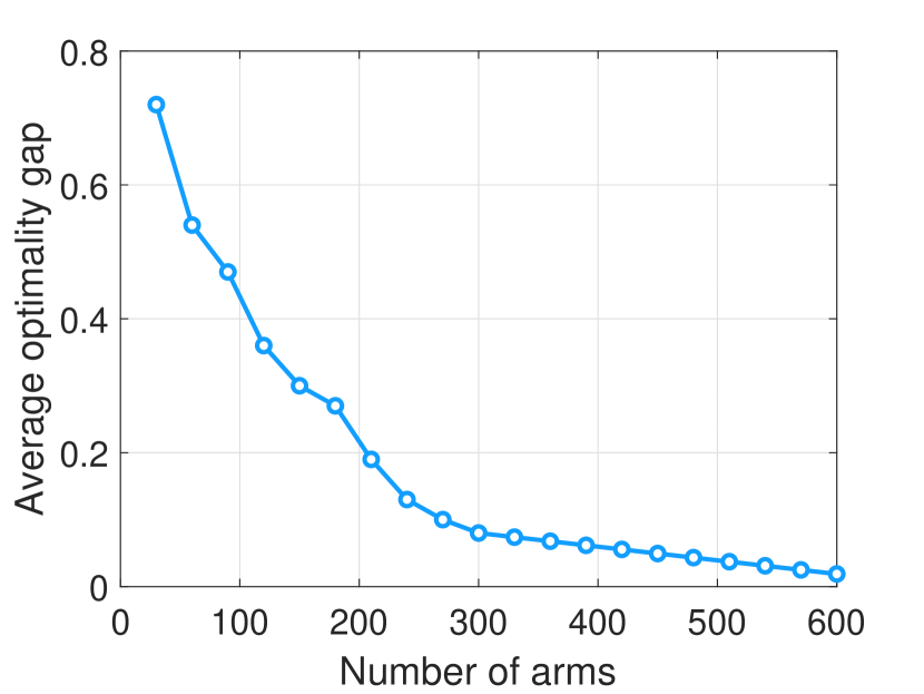
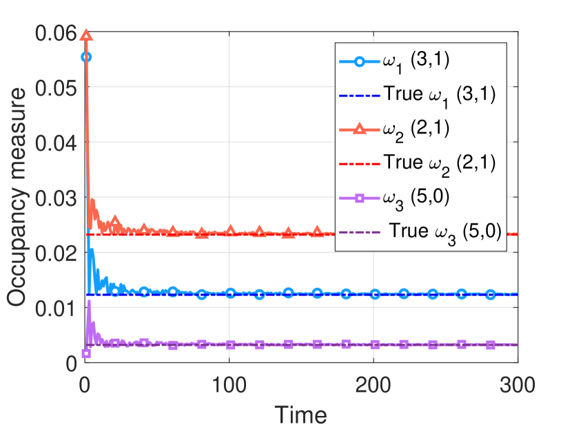
Using the synthetic trace setting in Sectionย Experiments, we verify the asymptotic optimality and global attractor assumption. We vary the number of arms from 30 to 600, and keep the budget as $\frac{1}{3}$ of the number of arms.

Asymptotic Optimality. We first validate the asymptotic optimality of FairRMAB index policy. In particular, we define the difference of average reward obtained by FairRMAB index policy with that from the theoretical upper bound solved from the LPย (36)-(40). We call the ratio between this award difference and the number of arms as optimality gap. From Figureย 9, we observe that as the number of arms increases, the optimality gap decreases significantly and closes to zero. This verifies the asymptotic optimality in Theoremย 3.

Global Attractor. As indicated in Remarkย 4, the asymptotic optimality of our FairRMAB index policy is under the definition of global attractor as in state of the arts. In Figureย 9, we randomly pick three state-action pairs $(3,1),(2,1)$ and $(5,0)$ for illustration. It is clear that the occupancy measure of arm 1 for state-action pair $(3,1)$ indeed converges. Similarly for arm 2 with state-action pair $(2,1)$ and for arm 3 with state-action pair $(5,0)$. Therefore, the convergence indeed occurs for our FairRMAB index policy and hence we verify the global attractor condition.

Appendix G Additional Experimental Details

Continuous Positive Airway Pressure Therapy (CPAP)

We study the CPAP as in (Kang etย al. 2013; Herlihy etย al. 2023; Li and Varakantham 2022b), which is a highly effective treatment when it is used consistently during the sleeping for adults with obstructive sleep apnea. The state space is ${1,2,3}$, which represents low, intermediate and acceptable adherence level respectively. Based on their adherence behaviour, patients are clustered into two groups, with the first group named โ€œAdherenceโ€ and the second โ€Non-Adherenceโ€. The difference between these two groups reflects on their transition probabilities, as in Figures. 10- 11. Generally speaking, the first group has a higher probability of staying in a good adherence level. From each group, we construct 10 arms , whose transition probability matrices are generated by adding a small noise to the original one. Actions such as text patients/ making a call/ visit in person will cause a 5% to 50% increase in adherence level. The budget is set to $B=5$ and the fairness constraint is set to be a random number between [0.1, 0.7]. The objective is to maximize the total adherence level.

PASCAL Recognizing Textual Entailment task (PASCAL-RTE1)

This is a task aims to infer hypothesis as in (Snow etย al. 2008). In each question, the annotator is provided with two sentences and tasked with making a binary choice regarding whether the second hypothesis sentence can be inferred from the first. For example, โ€œEgyptian television will make a series about Moslems, Copts and Boutros Boutros Ghaliโ€ can be inferred from โ€œEgyptian television is preparing to film a series that highlights the unity and cohesion of Moslems and Copts as the single fabric of the Egyptian society, exemplifying in particular the story of former United Nations Secretary-General Boutros Ghaliโ€. Due to carelessness or lack of background information, the annotator may not label correctly. The 10 workers we pick have worker id (A11GX90QFWDLMM, A14WWG6NKBDWGP, A151VN1BOY29J1, A15MN5MDG4D7Q9, A19PMUTQXDIPLZ, A1CP0KZJS5LSIF, A1DCEOFAUIDY58, A1IPO1FAD1A60X, A1LY3NJTYW9TFF, A1M0SEWUJYX9K0). The โ€œsuccessful annotation probabilityโ€ for each worker is averaged from all tasks, which is (0.495, 0.45, 0.4, 0.3, 0.6, 0.55, 0.65, 0.5, 0.54, 0.37). The state space is $\{0,1\}$, action space is $\{0,1\}$. The number of arms is $N=10$ and budget is set to $B=3$. We set $\eta=0.05$ for all arms.

Land Mobile Satellite System (LMSS)

We consider a similar setting as in (Wang, Huang, and Lui 2020) but extend it to the setting with more arms. The land mobile satellite needs to point at different directions (elevation angles). Each elevation angle will result in different channel parameters, hence different transition probabilities. We pick communicating via S-band in the urban environment and the corresponding parameters of two state Markov chain representations on the channel model. State 1 is defined as Good state and state 2 as Bad. There are 4 arms in total, which represents $40^{\circ},60^{\circ},70^{\circ},80^{\circ}$ elevation angle. The transition probabilities can be found in Table 1, which can be found in Table III (Prieto-Cerdeira etย al. 2010). The state space is $\{0,1\}$, action space is $\{0,1\}$. The number of arms is $N=4$ and budget is set to $B=2$. We set $\eta=0.03$ for all arms.

Elevation angle $p_{1,1}$ $p_{1,2}$ $p_{2,1}$ $p_{2,2}$
$40^{\circ}$ 0.9155 0.0845 0.0811 0.9189
$60^{\circ}$ 0.9043 0.0957 0.2 0.8
$70^{\circ}$ 0.9155 0.0845 0.2069 0.7931
$80^{\circ}$ 0.9268 0.0732 0.2667 0.7333
Table 1: Transition probability matrix of LMSS
$3$ $1$ $2$ $0.0385$ $0.0257$ $0.9615$ $0.9498$ $0.0245$ $1$
Figure 10: Transition diagram for CPAP Cluster 1
$3$ $1$ $2$ $0.7427$ $0.2323$ $0.1835$ $0.0741$ $0.6657$ $0.1020$ $0.4967$ $0.3399$ $0.1634$
Figure 11: Transition diagram for CPAP Cluster 2