FCBench: Cross-Domain Benchmarking of Lossless Compression for Floating-Point Data [Experiment, Analysis & Benchmark]

Abstract.

While both the database and high-performance computing (HPC) communities utilize lossless compression methods to minimize floating-point data size, a disconnect persists between them. Each community designs and assesses methods in a domain-specific manner, making it unclear if HPC compression techniques can benefit database applications or vice versa. With the HPC community increasingly leaning towards in-situ analysis and visualization, more floating-point data from scientific simulations are being stored in databases like Key-Value Stores and queried using in-memory retrieval paradigms. This trend underscores the urgent need for a collective study of these compression methods’ strengths and limitations, not only based on their performance in compressing data from various domains but also on their runtime characteristics. Our study extensively evaluates the performance of eight CPU-based and five GPU-based compression methods developed by both communities, using 33 real-world datasets assembled in the Floating-point Compressor Benchmark (FCBench). Additionally, we utilize the roofline model to profile their runtime bottlenecks. Our goal is to offer insights into these compression methods that could assist researchers in selecting existing methods or developing new ones for integrated database and HPC applications.

PVLDB Reference Format:
FCBench. PVLDB, 17(7): XXX-XXX, 2024.
doi:XX.XX/XXX.XX

PVLDB Artifact Availability:
The source code, data, and/or other artifacts have been made available at %leave␣empty␣if␣no␣availability␣url␣should␣be␣sethttps://github.com/hipdac-lab/FCBenchh.

1. Introduction

Floating-point data is widely used in various domains, such as scientific simulations, geospatial analysis, and medical imaging (Habib et al., 2016; Saeedan and Eldawy, 2022; Fout and Ma, 2012). As the scale of these applications increases, compressing floating-point data can help reduce data storage and communication overhead, thereby improving performance (Roth and Van Horn, 1993).

Why lossless compression? Using a fixed number of bits (e.g., 32 bits for single-precision data) to represent real numbers often results in rounding errors in floating-point calculations (Goldberg, 1991). Consequently, system designers favor using the highest available precision to minimize the problems caused by rounding errors (Rubio-González et al., 2013). Similarly, due to concerns about data precision, lossless compression is preferred over lossy compression, even with lower compression ratios, when information loss is not tolerable.

For instance, medical imaging data is almost always compressed losslessly for practical and legal reasons, while checkpointing for large-scale HPC simulations often employs lossless compression to avoid error propagation (Fout and Ma, 2012). Lossless compression is also essential for inter-node communication in a majority of distributed applications (Knorr et al., 2021b). This is because data is typically exchanged between nodes at least once per time step. Utilizing lossy compression would accumulate compression errors beyond acceptable levels, ultimately impacting the accuracy and correctness of the results. Another example is astronomers often insist that they can only accept lossless compression because astronomical spectra images are known to be noisy (Stockman, 1999; Du and Ye, 2009). With the background (sky) occupying more than $95\%$ of the images, lossy compressions would incur unpredictable global distortions (Oseret and Timsit, 2007).

1.1. Study Motivation

Both the HPC and database communities have developed lossless compression methods for floating-point data. However, there are fundamental differences between the floating-point data of these two domains. Typically, numeric values stored in database systems do not necessarily display structural correlations except for time-series data. In contrast, HPC systems often deal with structured high-dimensional floating-point data produced by scientific simulations or observations, such as satellites and telescopes. The result is that the two communities have developed floating-point data compression methods for different types of data within their respective domains. Naturally, an intriguing question arises: Can the compression methods developed in one community be applied to the data from the other community, and vice versa?

The urgency to answer this question arises from the growing trend of utilizing database tools on HPC systems. Practical use cases include in-situ visualization, which allows domain scientists to monitor and analyze large scientific simulations. For instance, Grosset and Ahrens developed Seer-Dash, a tool that utilizes Mochi’s Key-Value storage microservice (Ross et al., 2020) and Google’s LevelDB engine (Lev, 2011) to generate in-situ visualizations for the HACC simulation (Habib et al., 2016). color=blue!40]R1
W4

To this end, we view the previously isolated evaluation of compression methods in each community on their data as a shortcoming. In this paper, we survey 13 CPU- and GPU-based lossless floating-point data compression software from both communities. We evaluate their performances on 33 datasets from HPC, time-series, observation, and database transaction domains to fill the gap, while also profiling their runtime characteristics. We aim to provide an efficient methodology for future HPC and database developers to select the most suitable compressor for their use case/application, thereby reducing the cost of trial and error.

1.2. Our Contributions

• We present an experimental study of 13 lossless compression methods developed by the database and HPC communities for floating-point data.

• We evaluate the performance of these 13 compression methods based on a wide variety of 33 real-world datasets, covering scientific simulations, time-series, observations, and database transaction domains. This helps to refresh our understanding of the selected methods, as they were previously evaluated only within their own data domains.

• We investigate the compression performance with different block/page sizes and measure the query overhead on a simulated in-memory database application. This provides insights for database developers to employ suitable compression methods.

• We utilize the roofline model (Williams et al., 2009) to assess the runtime characteristics of selected algorithms regarding memory bandwidth utilization and computational operations, enabling potential to identify areas for performance enhancement.

• We employ statistical tools to recommend the most suitable compression methods, considering various data domains, and considering both the end-to-end time and query overheads.

Paper organization. The rest of this paper is organized as follows. In §2, we present background about floating-point data, lossless compression techniques, and previous survey works. In §3 and §4, we survey eight CPU-based and five GPU-based methods, respectively. In §5 and 6, we present the benchmarking methodology, experiment setup, and results. In §7, we summarize our findings and lessons. In §8, we conclude the paper and discuss future work.

2. Background and Related Work

We introduce the background on floating-point data representation, lossless compression of floating-point data, and related studies.

2.1. Floating-point Data

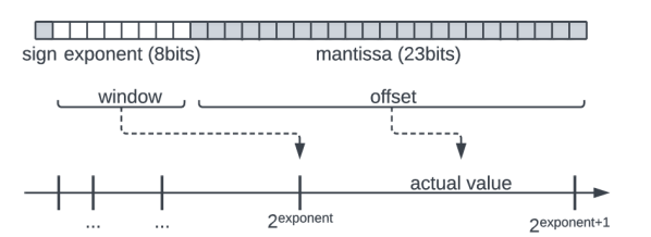
Figure 1. Single-precision format of the IEEE 754 standard.

The IEEE 754 standard  (Kahan, 1996) defined floating-point data to be in 32-bit single word and 64-bit double word format. Figure 1 illustrates the single-precision format: one bit for the positive or negative sign, 8 bits for the exponent, and 23 bits for the mantissa. The double-precision format includes one sign bit, 11 exponent bits, and 52 mantissa bits. The actual value of a floating-point datum is formulated as: $\text{x}=(-1)^{\text{sign}}\times 2^{(\text{exponent}-\text{bias})}\times 1.\text{mantissa}$.

2.2. Lossless Compression of Floating-point Data

Lossless compression encodes the original data without losing any information. It is, therefore, used to compress text, medical imaging and enhanced satellite data (Sayood, 2017), where information loss is not acceptable. Compression algorithms first identify the biased probability distribution, such as repeated patterns, and then encode the redundant information with reduced sizes. Some widely used encoding methods are listed below.

1. Run-length coding replaces a string of adjacent equal values with the value itself and its count.

2. Huffman coding builds optimal prefix codes to minimize the average length (Blelloch, 2001), based on the input data distribution.

3. Arithmetic coding uses cumulative distribution functions (CDF) to encode a sequence of symbols. It is more efficient than Huffman coding with increasing sequence length (Sayood, 2017).

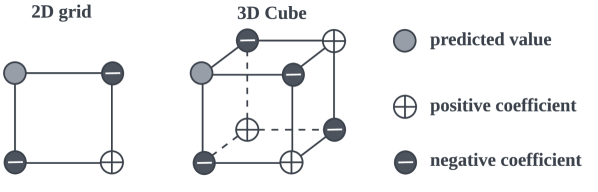
Figure 2. The Lorenzo transform and hypercubes.

2.3. The Lorenzo Transform

Data values from scientific simulations or sensors tend to correlate with neighboring values (Knorr et al., 2021b). The Lorenzo predictor (Ibarria et al., 2003) can leverage such structural dependencies to encode with fewer bits (Cayoglu et al., 2019). Figure 2 shows the value on a corner of a 2D grid or 3D cube can be estimated by the neighboring corners: $\hat{x}=\sum x_{\text{odd}}-\sum{x_{\text{even}}}$. The 2D or 3D structures can be generalized to high-dimensional hypercubes in the Lorenzo transform.

2.4. Friedman Test and Post-hoc Tests

The machine learning community has long been embracing statistical validation to compare algorithms on a number of test data sets. According to the theoretical and empirical guidance by Demšar, the Friedman test and corresponding post-hoc analysis overcome the limitations associated with using averaged metrics. These statistical tests are suitable to apply when the number of algorithms $k>5$ and the number of datasets $N>10$. color=blue!40]R4
W5 The Friedman test (Demšar, 2006) compares the averaged ranks to find if all the algorithms are equivalent. The post-hoc Nemenyi test computes critical differences (CD) of averaged ranks. Finally, the CD diagram displays algorithms ordered by their average rank and groups of algorithms between which there is no significant difference.

2.5. Related Prior Surveys

Previous surveys on data compression for databases and HPC applications have been conducted.  Wang et al. comprehensively studied 9 bitmap compression methods and 12 inverted list compression methods for databases on synthetic and real-world datasets (Wang et al., 2017). However, bitmap and inverted list methods only compress categorical and integer values. Son et al. studied 8 lossless and 4 lossy compression methods for scientific simulation checkpointing in the exascale era (Son et al., 2014). They favored lossy compression algorithms for scientific simulations checkpointing but did not consider the situations when lossless compression is required. Lindstrom compared 7 lossless compression methods but only tested them on one turbulence simulation dataset (Lindstrom, 2017). Although the evaluation metrics of space and time were common in previous studies from both communities, the database community distinguished itself by investigating the influence of compressors on query performances. Compared with previous benchmarks, our study stands out in three key aspects. color=blue!40]R1
W1 First, we include more recent compressors, covering multiple domains for a comprehensive evaluation of both software and datasets. Second, we offer insights not only from the algorithm design perspective but also from the standpoint of system architecture. Third, we employ a collection of tools to ensure a fair comparison of the selected methods. Specifically, we use statistical tests for rankings and recommendations, a simulated in-memory database for evaluating query performance, and the roofline model to investigate runtime bottlenecks.

Table 1. Summary of our studied lossless compression methods^∗

year

domain

precision∗∗

arch.

parallel impl.

language

trait

availability

fpzip (Lindstrom and Isenburg, 2006)

2006

HPC

S,D

CPU

serial

C++

Lorenzo

open-source

pFPC (Burtscher and Ratanaworabhan, 2009)

2009

HPC

D

CPU

threads

C

prediction

open-source

bitshuffle::LZ4 (Masui et al., 2015)

2015

HPC

S,D

CPU

SIMD + threads

C+Python

transform + dict.

open-source

bitshuffle::zstd (Masui et al., 2015)

2015

HPC

S,D

CPU

SIMD + threads

C+Python

transform + dict.

open-source

Gorilla (Pelkonen et al., 2015)

2015

Database

D

CPU

serial

go

delta

open-source

SPDP (Claggett et al., 2018)

2018

HPC

S,D

CPU

serial

C

dictionary

open-source

ndzip-CPU (Knorr et al., 2021a)

2021

HPC

S,D

CPU

SIMD + threads

C++

transform+Lorenzo

open-source

BUFF (Liu et al., 2021)

2021

Database

S,D

CPU

serial

rust

delta

open-source

Chimp(Liakos et al., 2022)

2022

Database

S,D

CPU

serial

go

delta

open-source

GFC (O’Neil and Burtscher, 2011)

2011

HPC

D

GPU

SIMT

CUDA C

delta

open-source

MPC (Yang et al., 2015)

2015

HPC

S,D

GPU

SIMT

CUDA C

transform+delta

open-source

nvcomp::LZ4 (NVIDIA, 2023)

2020

general

S,D

GPU

SIMT

CUDA C++

transform + dict.

proprietary

nvcomp::bitcomp (NVIDIA, 2023)

2020

general

S,D

GPU

SIMT

CUDA C++

transform + prediction

proprietary

ndzip-GPU (Knorr et al., 2021b)

2021

HPC

S,D

GPU

SIMT

SYCL C++

transform + Lorenzo

open-source

Dzip (Goyal et al., 2021)

2021

general

S,D

GPU

SIMT

Pytorch

prediction

open-source

$*$ bitshuffle methods (LZ4 and zstd) and nvcomp methods (LZ4 and bitcomp) are all listed separately. $**$ S, D stand for single-/double-precision.

3. CPU-based compression methods

In this section, we describe eight CPU-based lossless compression methods. The first five are serial methods, and the last three are parallel methods. For each method, we introduce its computational workflow along with noteworthy features. Table 2.5 summarizes all the studied methods. Their timeline is shown in Figure 3.

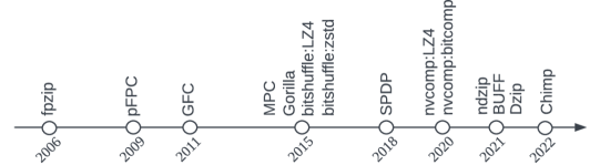
Figure 3. Timeline of studied compression methods.

3.1. fpzip

fpzip (Lindstrom and Isenburg, 2006) is a prediction-based compression algorithm that provides both lossless and lossy compression on the single- and double-precision floating-point data for scientific simulations.

Workflow: (1) fpzip uses the Lorenzo predictor (Ibarria et al., 2003) to predict the value of a hypercube corner from its previously encoded neighboring corners. (2) The predicted and actual floating-point values are mapped to sign-magnitude integers to compute the residual. (3) The integer residuals’ sign and leading zeros are symbols and encoded by a fast range coding method (Martin, 1979). (4) The remaining non-zero bits are copied verbatim.

Insights: color=blue!40]R1 W3For fpzip to achieve a better compression ratio, users should provide the Lorenzo predictor with the correct data dimensionality to predict with the hypercubes. Note that fpzip does not use parallel computing techniques.

3.2. SPDP

SPDP (Claggett et al., 2018) (Single Precision Double Precision) is a dictionary-based lossless compression algorithm for both precisions. It can work as an HDF5 filter (hdf, 2023) or a standalone compressor.

Workflow: SPDP is synthesized from three transform components to expose better data correlations and a reducer component to encode the transformed values. After sweeping over a total of 9,400,320 combinations on 26 scientific datasets, the authors selected the following four components that rendered the best compression ratios: (1) LNVs2 subtracts the last $2^{nd}$ byte value from the current byte value and emits the residual. (2) DIM8 groups the most significant bytes of the residuals, followed by the second most significant bytes, etc. This puts the exponent bits into consecutive bytes. (3) LNVs1 computes the difference between the previously grouped consecutive bytes. (4) LZa6 is a fast variant of the LZ77 (Ziv and Lempel, 1977) to encode the final residuals.

Insights: SPDP has the trade-off between compression ratio and throughput because LZa6 employs a sliding window to encode the positions and lengths of matched patterns. Larger sliding window sizes can increase the compression ratio with the cost of decreased throughput due to prolonged searching time.

3.3. BUFF

BUFF (Liu et al., 2021) is a delta-based compression algorithm for low-precision floating-point data, commonly used in server monitoring and IoT (Internet of Things) devices. Two features distinguish BUFF from other methods in this survey. (1) Without precision information, BUFF essentially becomes a lossy compressor. (2) BUFF can directly query byte-oriented columnar encoded data without decoding. This capability allows BUFF to achieve a speedup ranging from 35x to 50x for selective and aggregation filtering.

Table 2. Number of bits needed for targeted precision in BUFF.

Precision	1	2	3	4	5	6	7	8	9	10
Bits needed	5	8	11	15	18	21	25	28	31	35

Workflow: (1) BUFF splits the input values into integer and fractional components. (2) It then uses a look-up table (Table 2) to keep the most significant bits of the mantissa part and discard the trailing bits. (3) BUFF computes the difference between the current and minimal values. (5) BUFF uses padding to encode the integer and fraction parts into a multiple of bytes. Each byte unit is treated as a sub-column and stored together to enable query operations. (6) The value range and precision information are saved as metadata and compressed data for decompression.

Insights: BUFF’s compression ratio is sensitive to the value ranges and outliers. It does not employ parallel processing. The byte-column query follows the pattern match method. Assume each data point $x$ is encoded and saved in sub-columns $x_{1},x_{2},...,x_{k}$. To perform a predicate $x==C$, BUFF translates $C$ into sub-columns $C_{1},C_{2},...,C_{k}$ and evaluates the equal operator on the sub-columns one at a time. BUFF will skip a record once a sub-column is disqualified ($x_{i}!=C_{i}$).

3.4. Gorilla

Gorilla (Pelkonen et al., 2015) is a delta-based lossless compression algorithm to compress the timestamps and the data values for the in-memory time series database used at Facebook.

Workflow: Given that time series data are often represented as pairs of a timestamp and a value, Gorilla uses two different methods: (1) It uses delta-of-delta to compress timestamps. With the fixed interval of time series data, the majority of timestamps can be encoded as a single bit of 0. (2) For floating-point data values, Gorilla conducts XOR operations on the current and previous values and encodes the residuals from the XOR operation. (3) Gorilla uses a single bit $C=\texttt{0}$ to store all-zero residuals; $C=\texttt{10}$ is used to store the actual meaningful bits when the nonzero bits of the residual fall within the block bounded by the previous leading zeros and trailing zeros; $C=\texttt{11}$ uses $5$ bits for the length of leading-zeros, $6$ bits for the length of meaningful bits and then the actual residual.

Insights: Gorilla’s performance is sensitive to the data patterns. The overhead of control bits becomes high when data values change frequently. Gorilla does not employ parallel computing techniques.

3.5. Chimp

Chimp (Liakos et al., 2022) is a lossless compression algorithm to compress floating-point values of time series data. Based on Gorilla’s (Pelkonen et al., 2015) workflow, Chimp redesigned the control bits to improve compression ratio when the trailing zeros of XORed residuals are less than $6$. Furthermore, Chimp computes the best XORed residual (having the highest number of trailing zeros) from the $128$ previous values. In other words, Chimp is a prediction-based method with a sliding window ((Burtscher and Ratanaworabhan, 2007, 2009)).

Workflow: (1) Chimp maintains evicting queues to store 128 previous values grouped by their less significant bits. This enables Chimp to get more trailing zeros from the XORed residuals than Gorilla. (2) Chimp uses control bits $C=\texttt{00}$ to encode all-zero residuals; For $C=\texttt{01}$, Chimp uses 3 bits to encode the length of leading zeros and 6 bits to encode the length of meaningful bits. Then it stores the meaningful bits; For $C=\texttt{10}$, the current length of leading zeros equals the previous length of leading zeros, so Chimp directly stores the meaningful bits; For $C=\texttt{11}$, Chimp uses 3 bits to encode the length of leading zeros, then stores the meaningful bits.

Insights: Using a sliding window allows Chimp to achieve a higher compression ratio when data values are more random. However, the overhead of looking up the sliding window also decreases Chimp’s compression throughput compared with Gorilla’s.

3.6. pFPC

pFPC (Burtscher and Ratanaworabhan, 2009) is a prediction-based algorithm that losslessly compresses double-precision scientific simulation data in parallel.

Workflow: (1) pFPC stores historical value sequences in two hash tables and predicts current values by looking up the hash tables. (2) The residuals are computed from the XOR operation between the actual and predicted values. (3) The leading zeros of the XORed result and the selected hash predictor are encoded with 4 bits. (4) The nonzero residual bytes are copied.

Insights: pFPC utilizes parallel computing to increase the overall throughput. The original data is partitioned into chunks and distributed across multiple CPU threads (default 8 pthreads)color=blue!40]R4 W1. However, there exists a trade-off between compression ratio and throughput. Given that high-dimensional scientific data often exhibits higher correlation along the same dimension, pFPC prefers to align the number of threads with the data dimensionality. With a large number of threads and big chunk sizes, mixing values from multiple dimensions can decrease the compression ratio. Thus, pFPC requires data dimensionality as input parameters and typically does not fully utilize multi-threading capacity to align with the data dimensionality.

3.7. Bitshuffle

Bitshuffle (Masui et al., 2015) is a data transform in itself. The algorithm can expose the data correlations within a subset of bits in a byte to improve the compression ratio for downstream encoders.

Workflow: (1) Bitshuffle splits the input data into blocks and distributes the blocks among threads. On each thread, a block’s bits are arranged into a $m\times n$ matrix, where $m$ is the number of values in a block, and $n$ is the data element size (32 or 64 bits). Then, it performs a bit-level transpose to get a $n\times m$ matrix, where the i^th ($1\leq i\leq n$) bits are combined into bytes. (2) Bitshuffle uses other methods, such as LZ4 and zstd, to encode the transposed data.

Insights: Bitshuffle employs SSE2 and AVX2 vectorized instruction sets for parallelized transforms. Although larger blocks will increase the compression ratios, the default block size is set to $4096$ bytes to ensure that Bitshuffle can fit data into the L1 cache. LZ4 and zstd are then applied to the cached data to improve performance.

3.8. ndzip-CPU

ndzip (Knorr et al., 2021a) is a prediction-based lossless compression algorithm. The CPU implementation uses SIMD instructions and thread-level parallelism to achieve high throughput.

Workflow: (1) ndzip divides data into blocks, with each block corresponding to a hypercube containing 4096 elements. (2) A multidimensional Integer Lorenzo transform computes the residuals within each block. (3) The residuals are divided into chunks of $32$ single-precision or $64$ double-precision values and performs bit-transpose operations. (4) The zero-words in the transposed chunks are removed. The positions of zero-words are encoded with 32- or 64-bit bitmap headers, and the non-zero words are copied.

Insights: ndzip employs multi-level parallel computing to achieve high throughputs. The hypercubes are independently compressed using thread-level parallelism, while each hypercube’s transformation, transposition, and encoding leverage SIMD vector instructions.

4. GPU-based Compression Methods

4.1. GFC

GFC (O’Neil and Burtscher, 2011) is a delta-based compression algorithm for double-precision floating-point scientific data. GFC leverages the massive GPU parallelism to achieve high compression/decompression throughput.

Workflow: (1) GFC divides input data into chunks equal to the number of GPU warps, each consisting of 32 threads. These chunks are further divided into subchunks of $32$ double-precision values and compressed independently. (2) GFC computes residuals by subtracting the last value of the previous subchunk from the current subchunk. (3) GFC encodes the sign and leading zeros with 4 bits followed by the non-zero residual bytes. These operations are performed in parallel across GPU warps.

Insights: GFC sets the size of subchunks to $32$ to align with the number of GPU threads in a warp. However, the delta-based predictor sacrifices accuracy to accommodate multidimensional data within fixed-sized (256 Bytes) subchunks. This is due to the computation of all residuals for the current 32 values by subtracting the last value from the previous 32. Another limitation of GFC is that the input data size cannot exceed $512$ MB based on the hardware available during their research.

4.2. MPC

MPC (Yang et al., 2015), which stands for Massive Parallel Compression, is a synthesized delta-based lossless compression algorithm for floating-point data. It is constructed from four components following the process described in §3.2. The number of combinatorial search spaces for MPC is $138,240$.

Workflow: MPC divides input data into chunks of 1024 elements and processes them in parallel. The pipeline consists of four components: (1) LNV6s computes the residual by subtracting the $6^{th}$ prior value in the same chunk from the current value. (2) BIT reorganizes the data chunks by emitting the most significant bit of each word first (packing them into words), followed by the second most significant bits, and so on. This is essentially the same operation of Bitshuffle (Masui et al., 2015). (3) LNV1s computes differences between consecutive words from the BIT transform. Finally, (4) ZE outputs a bitmap to indicate zero values in the chunk and copies the non-zero values after the bitmap.

Insights: MPC resembles ndzip in the entire pipeline, except for using the delta-based predictor to replace the Lorenzo prediction. The input word size (single- or double-precision) information is important so that LNV6s computes the correct residuals. MPC demonstrated that a delta-based predictor could achieve good compression ratios when combined with data transform components.

4.3. nvCOMP

nvCOMP (NVIDIA, 2023) is a CUDA library by NVIDIA to provide APIs of compressors and decompressors. In the latest version (2.4), nvCOMP includes $8$ compression algorithms. We include nvCOMP::LZ4 because it achieves the highest compression ratio among the 8 compressors. Similarly, we include nvCOMP::bitcomp for it has the highest compression/decompression throughput.

Workflow: nvCOMP has been proprietary software since version 2.3, and NVIDIA does not describe the detailed workflow for each compression method.

Insights: nvCOMP::LZ4 and nvCOMP::bitcomp do not require extra input parameters such as dimensional information.

4.4. ndzip-GPU

ndzip-GPU (Knorr et al., 2021b) is the GPU-based parallelization scheme for the ndzip algorithm in §3.8. While the algorithm remains the same, the GPU implementation further improves parallelism by distributing transforming and residual coding among up to 768 threads.

Workflow: The compression pipeline of ndzip-GPU is the same as the CPU implementation: (1) Divide data into hypercubes, (2) Compute residuals using the Lorenzo predictor, (3) Perform bit-transposition, (4) Remove zero-words, output the bit-map header and uncompressed non-zeros.

Insights: ndzip-GPU first writes encoded chunks to a global scratch to guarantee the order of variable-length encoded chunks. After computing a parallel prefix sum to obtain the offsets for all chunks, ndzip copies the encoded chunks from scratch memory to the output stream. By retrieving the offsets for each compressed block, the decompression is fully block-wise parallel without synchronization.

4.5. Dzip

While Dzip (Goyal et al., 2021) is not developed by the HPC or database community, the Neural Network-based compression method represents an emerging direction. Therefore, we include this method to enrich our survey. Dzip is a general-purpose lossless compressor in contrast to the aforementioned floating-point oriented methods. It trains two recurrent neural network (RNN) models to estimate the conditional distribution for input data symbols and encodes them with an arithmetic encoding method.

Workflow: (1) An RNN-based bootstrap model is trained for multiple passes. (2) Dzip trains a larger supporter model and the bootstrap model in a single pass to predict the conditional probability of the current symbol. The supporter models are discarded after encoding to save disk space. (3) Dzip retrains a new supporter model combined with the bootstrap model in one pass during decoding. This supporter model is again discarded later.

Insights: The bootstrap model is trained and saved. However, the supporter model needs retraining for unseen datasets. Although Dzip is faster than other NN-based compressors, such as NNCP (Bellard, 2021) and CMIX (Knoll, 2023), its compression speed is about several KB/s. Thus, NN-based compression methods are still not practical for applications at the time of our survey.

5. Benchmark Methodology and Setup

In this section, we present our benchmarking methodology and experimental setups, including test datasets, software and hardware configurations, and evaluation metrics.

5.1. Our Methdology

This benchmarking aims to enrich our understanding of these compression algorithms’ performance from various perspectives. Our benchmarking study encompasses three aspects.

5.1.1. The compression aspect:

We evaluate the selected algorithms with generic metrics: compression ratio, (de)compression throughputs, end-to-end wall time, the effect of dimensionality parameters, and scalability of parallel compression. For fair comparisons, we perform statistical tests on the rankings.

5.1.2. The database query aspect:

We adopt a micro-benchmarking approach (Lissandrini et al., 2018; Boral and Dewitt, 1984) to swiftly evaluate query performance with compression. Rather than analyzing queries in a comprehensive database system, we develop a tool to simulate an in-memory database and investigate three primitive operations: file I/O, data decoding, and full table scan query. color=blue!40]R1 W2 More concretely, we depict an HPC system in Figure 4 that reads Hierarchical Data Format 5 (HDF5) (Folk et al., 2011) files from the disk into Pandas (Snider and Swedo, 2004) dataframes in memory and performs the queries on these in-memory dataframes. This simulated database enables us to quickly check the compression performance with various block sizes and measure the decompression overhead for query operations under the database context.

Our simulated tool has limitationscolor=blue!40]R1 W2 in accurately reflecting the true query performance of integrated compression methods in a real database system. This is mainly because a full table scan oversimplifies the process compared to more complex operations like join and update queries in in-situ visualization applications. it does help to bypass the substantial engineering efforts needed to integrate compressors into an actual database system, aiding in the selection of the best-fit method.

5.1.3. The system design aspect:

We use the roofline model (Williams et al., 2009) to identify potential bottlenecks, such as arithmetic intensity and memory bandwidth, for future compression algorithm developers.

Figure 4. Integrating HPC and database with HDF5 and Dataframes.

5.2. Evaluation Metrics

We use the compression ratio (CR), compression throughput (CT), and decompression throughput (DT) to measure the compression performance. They are calculated as follows.

$$\text{CR}=\frac{\text{orig size}}{\text{comp size}},\quad\text{CT}=\frac{\text{orig size}}{\text{comp time}},\quad\text{DT}=\frac{\text{orig size}}{\text{decomp time}}$$

For fpzip, pFPC, Gorilla, SPDP, ndzip (CPU and GPU), BUFF, Chimp, GFC, and MPC, we measured the times by adding instructions before and after the compression/decompression function to exclude the I/O. For bitshuffle (LZ4 and zstd) and nvcomp (LZ4 and bitcomp), we directly reported the timings and compression ratio obtained from their built-in benchmark functions. We repeated each method on the selected datasets ten times and reported each dataset’s average compression ratios, run times, and throughputs. We used the harmonic mean of compression ratios and arithmetic mean of throughputs to evaluate the overall performance.d.

5.3. Datasets

We choose 33 open datasets from four domains, shown in Table 5.3. The datasets include (1) scientific simulation data from Scientific Data Reduction Benchmarks (Zhao et al., 2020) and (Knorr et al., 2020); (2) time series data such as sensor streams, stock market, and traffic data which typically require fewer precision digits; (3) observation data such as HDR photos and telescope images; (4) simulated data generated from the Transaction Processing Performance Council Benchmark (TPC) (Council, 2005), including numeric columns extracted from the TPC-H, TPCX-BB, and TPC-DS transactions. Although the largest data size of 4GB in our selection is much small for a typical HPC application, it is a common workload of a time step for in-situ analysis (Grosset and Ahrens, 2021) and has been evaluated by many benchmark studies (Zhao et al., 2020; Knorr et al., 2020).color=blue!40]R4 W4

Table 3. Evaluated floating-point datasets.

domain & name					type∗	size in bytes	entropy	extent
HPC msg-bt (BURTSCHER, 2009)	D	266,389,432	23.67	33298679 (1D)
HPC num-brain (BURTSCHER, 2009)	D	141,840,000	23.97	17730000 (1D)
HPC num-control (BURTSCHER, 2009)	D	159,504,744	24.14	19938093 (1D)
HPC rsim (Thoman et al., 2020)	S	94,281,728	18.50	2048$\,\times\,$11509 (2D)
HPC astro-mhd (Kissmann et al., 2016)	D	548,458,560	0.97	130$\,\times\,$514$\,\times\,$1026 (3D)
HPC astro-pt (Huber et al., 2021)	D	671,088,640	26.32	512$\,\times\,$256$\,\times\,$640 (3D)
HPC miranda3d (Zhao et al., 2020)	S	4,294,967,296	23.08	1024$\,\times\,$1024$\,\times\,$1024 (3D)
HPC turbulence (Klacansky, 2009)	S	67,108,864	23.73	256$\,\times\,$256$\,\times\,$256 (3D)
HPC wave (Thoman et al., 2019)	S	536,870,912	25.27	512$\,\times\,$512$\,\times\,$512 (3D)
HPC hurricane (Zhao et al., 2020)	S	100,000,000	23.54	100$\,\times\,$500$\,\times\,$500 (3D)
TS citytemp (Kaggle, 2019)	S	11,625,304	9.43	2906326 (1D)
TS ts-gas (Fonollosa et al., 2015)	S	307,452,800	13.94	76863200 (1D)
TS phone-gyro (Stisen et al., 2015)	D	334,383,168	14.77	13932632$\,\times\,$3 (2D)
TS wesad-chest (Schmidt et al., 2018)	D	272,339,200	13.85	4255300$\,\times\,$8 (2D)
TS jane-street (Kaggle, 2022b)	D	1,810,997,760	26.07	1664520$\,\times\,$136 (2D)
TS nyc-taxi (Kaggle, 2021)	D	713,711,376	13.17	12744846$\,\times\,$7 (2D)
TS gas-price (Kaggle, 2022a)	D	886,619,664	8.66	36942486$\,\times\,$3 (2D)
TS solar-wind (Kaggle, 2022c)	S	423,980,536	14.06	7571081$\,\times\,$14 (2D)
OBS acs-wht (MAST, 2023)	S	225,000,000	20.13	7500$\,\times\,$7500 (2D)
OBS hdr-night (Haven, 2018)	S	536,870,912	9.03	8192$\,\times\,$16384 (2D)
OBS hdr-palermo (Haven, 2020)	S	843,454,592	9.34	10268$\,\times\,$20536 (2D)
OBS hst-wfc3-uvis (MAST, 2023)	S	108,924,760	15.61	5329$\,\times\,$5110 (2D)
OBS hst-wfc3-ir (MAST, 2023)	S	24,015,312	15.04	2484$\,\times\,$2417 (2D)
OBS spitzer-irac (IRSA, 2023)	S	164,989,536	20.54	6456$\,\times\,$6389 (2D)
OBS g24-78-usb (MAST, 2023)	S	1,335,668,264	26.02	2426$\,\times\,$371$\,\times\,$371 (3D)
OBS jws-mirimage (MAST, 2023)	S	169,082,880	23.16	40$\,\times\,$1024$\,\times\,$1032 (3D)
DB tpcH-order (TPC, 2023b)	D	120,000,000	23.40	15000000 (1D)
DB tpcxBB-store (TPC, 2023c)	D	789,920,928	16.73	8228343$\,\times\,$12 (2D)
DB tpcxBB-web (TPC, 2023c)	D	986,782,680	17.64	8223189$\,\times\,$15 (2D)
DB tpcH-lineitem (TPC, 2023b)	S	959,776,816	8.87	59986051$\,\times\,$4 (2D)
DB tpcDS-catalog (TPC, 2023a)	S	172,803,480	17.34	2880058$\,\times\,$15 (2D)
DB tpcDS-store (TPC, 2023a)	S	276,515,952	15.17	5760749$\,\times\,$12 (2D)
DB tpcDS-web (TPC, 2023a)	S	86,354,820	17.33	1439247$\,\times\,$15 (2D)

$**$ S, D stand for single-/double-precision.

5.4. Friedman Test and Post-hoc Tests

Following recent survey works (Freeman et al., 2021; Holder et al., 2023), we apply the Friedman test and apply the CD diagram (Demšar, 2006) to compare the selected compression methods. We use $\alpha=0.05$, $k=13$, $N=33$ for the hypothesis test and compute the critical difference. color=blue!40]

W5

5.5. System Configuration

We evaluate the selected compression methods on a Chameleon Cloud (Keahey et al., 2020) compute node with two Intel Xeon Gold 6126 CPUs (2.6 GHz), 187 GB RAM and one Nvidia Quadro RTX 6000 GPU (24 GB VRAM). The node is configured with Ubuntu 20.04, GCC/G++ 9.4, CUDA 11.3, CMAKE 3.25.0, HDF5 1.14.1, and Python 3.8.

fpzip, pFPC, SPDP, ndzip-CPU are compiled with GCC/G++ $9.4$; nvCOMP::LZ4 and nvCOMP::bitcomp are executable binary files downloaded from the benchmark page; bitshuffle::LZ4 and bitshuffle+zstd are compiled with Python 3.8 and GCC 9.4; Gorilla and Chimp are integrated in influxdb, where they can be compiled with go 1.18.0 and rustc 1.53.0; BUFF is compiled with the nightly version of rust. GFC, MPC and ndzip-GPU are compiled with nvcc 11.3. Each C/C++ method was compiled with -O3 flag. When possible, we changed the compile flags for GPU-based methods to use the current GPU architecture -arch=sm_75.

6. Evaluation Results

In this section, we present the results following our evaluation methodology described in §5.1. We begin by discussing general compression performance, covering compression ratio, compression throughput, decompression throughput, and end-to-end wall time (including memory copy, especially for GPU-based compressors). This is followed by detailed discussions. Subsequently, we delve into the evaluation results related to compression performance in the context of databases. Finally, we present the findings from the roofline model.

6.1. General Compression Performance

We evaluate the compression algorithms using the following parameters: (1) the compression level, which is set for the best compression ratios (CRs), and (2) blocks/chunks, which are set to default sizes when applicable.

6.1.1. Compression Ratio

Figure 5 shows all measured compression ratios. The median is $1.16$ and outliers range from $2.0$ to $22.8$. Our experiments support previous study  (Lindstrom, 2017) that floating-point data is difficult to compress.

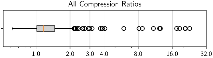
Figure 5. BoxPlot of compression ratios.

Figure 5(a) shows the compression ratios on datasets of different domains and data types. (1) The median compression ratio is 1.225 for single- and 1.202 for double-precision datasets. This result supports the study (Yang et al., 2015) that double-precision data are more challenging to compress. (2) Observation datasets (OBS) have the highest median compression ratio of $1.292$, followed by HPC, Time Series (TS), and Database (DB) datasets with those of $1.206$, $1.223$, and $1.080$. DB is the most difficult domain to compress.

(a) Data type and domains

(b) Prediction methods and hardware platforms

Figure 6. Compression ratios by data/methods groups.

Figure 5(b) shows the compression ratios of different groups of compression methods based on their predictors and hardware platforms. (1) Dictionary-based methods (bitshuffle::LZ4, bitshuffle+zstd, Chimp) achieve higher compression ratios than Lorenzo-based methods (fpzip, ndzip-CPU, ndzip-GPU) and Delta-based methods (Gorilla, GFC, and MPC). The median compression ratios for these three groups are 1.309, 1.219, and 1.116, respectively. (2) On the selected datasets, CPU-based methods exhibit higher compression ratios compared to GPU-based methods.

Analysis: color=blue!40]R1 W3(1) Except for BUFF, the selected algorithms compress either leading zeros or zero words. This is intuitive, as the exponents are more compressible. Double-precision data are less compressible due to their larger mantissa portion. (2) The OBS dataset achieves the best compression ratio as it consists of highly structured single-precision values. In contrast, the DB dataset is the most challenging to compress due to its lack of structural patterns. (3) Dictionary-based predictors outperform others because they search for patterns over a longer range. (4) CPU-based methods tend to use more dictionary-based predictors compared to GPU-based methods.

Takeaway: (1) Using single-precision for saving numeric values in databases is desirable. (2) Dictionary-based predictors perform better than delta- and Lorenzo-based predictors.

(a) Average compression ratios

(b) critical difference diagram on compression ratios

Figure 7. Compression ratios of different methods.

color=blue!40]R4 W5Table 6.1.1 shows the detailed CRs and Figure 6(a) shows their harmonic mean CRs. In Figure 6(b), we present the critical difference diagram, where the selected methods are ordered according to their average rankings (higher ranking is better) and cliques (a group of algorithms) are connected by a line representing the critical difference. We further observe: (1) The CD diagram shows no clear winner because bitshuffle+zstd is not significantly better than SPDP, although it has a significantly higher CR than ndzip-GPU. (2) GFC ranks the lowest but is not significantly lower than nvCOMP::bitcomp, gorilla, BUFF, and pFPC. (3) fpzip has the highest compression ratio on HPC datasets; nvCOMP::LZ4 works the best on Time series (TS); bitshuffle+zstd performs the best for Observation (OBS) datasets; Chimp performs the best on Database (DB) datasets. (4) CPU-based methods are more robust than GPU-based methods: $2.0\%$ of CPU experiments incurred runtime errors, while $7.3\%$ of the GPU experiments were killed by runtime errors.

Analysis: (1) Dictionary-based predictors not only help bitshuffle::zstd achieve the top rank in compression ratios (CRs), but they also assist Chimp128 in outperforming Gorilla. (2) Bit-level transpose operations can expose subtle patterns, such as identical i^th bits, benefiting both bitshuffle and MPC. (3) As described in §4.1, the less accurate predictor of GFC contributes to its lower ranking.

Takeaway: (1) Although the critical difference does not significantly distinguish bitshuffle::zstd from the rest in the group (including bitshuffle::Lz4, MPC, fpzip, nvCOMP::LZ4, Chimp128, and SPDP), it does highlight a direction for future research: exploring bit-level transposition and dictionary-based predictors to improve compression ratios. (2) For highly structured data from the HPC or OBS domains, delta- and Lorenzo-based compressors are comparable to, or even better than, dictionary-based compressors. (3) As numerical values in DB datasets lack structure, dictionary-based methods outperform delta- and Lorenzo-based methods.

Table 4. Compression ratios (i.e., $\text{original size}/\text{compressed size}$).

domain & name		pFPC	SPDP	fpzip	shf+ LZ4	shf+ zstd	ndzip -CPU	BUFF	Gorilla	Chimp	GFC	MPC	nv:: LZ4	nv:: btcmp	ndzip -GPU
HPC msg-bt	1.251	1.327	1.200	1.205	1.188	1.127	1.032	1.086	1.129	1.091	1.145	1.063	1.056	1.127
HPC num-brain	1.153	1.200	1.250	1.174	1.177	1.165	2.133	1.110	1.175	1.091	1.185	0.996	0.999	1.165
HPC num-control	1.036	1.011	1.120	1.114	1.117	1.109	2.207	0.980	1.057	1.013	1.108	1.013	1.009	1.109
HPC rsim	1.351	1.686	1.480	1.500	1.560	1.973	0.640	1.335	1.338	1.298	1.514	1.309	1.306	1.973
HPC astro-mhd	10.926	20.935	8.720	12.367	17.506	12.579	1.524	18.595	5.971	-	8.132	22.824	20.801	12.579
HPC astro-pt	1.285	1.398	1.200	1.202	1.214	1.423	2.000	1.032	1.223	-	1.224	0.996	0.999	1.423
HPC miranda3d	1.136	1.195	2.200	-	-	1.835	1.067	1.039	1.177	-	1.495	1.020	1.019	-
HPC turbulence	1.012	1.046	1.420	1.150	1.157	1.232	0.889	0.986	1.023	1.002	1.166	0.996	0.999	1.232
HPC wave	1.160	1.905	3.870	1.291	1.313	1.993	1.103	1.032	1.145	1.018	1.416	1.032	0.999	1.993
HPC hurricane	0.946	1.372	-	1.513	1.552	0.974	-	1.064	0.987	0.945	1.494	1.003	1.002	0.974
Domain-avg	1.229	1.381	1.601	1.447	1.468	1.450	1.149	1.161	1.232	1.059	1.399	1.167	1.131	1.420
TS citytemp	1.083	1.014	1.470	2.240	2.314	1.305	0.889	1.027	1.255	1.079	1.347	1.374	1.015	1.305
TS ts-gas	1.335	1.406	1.930	1.426	1.501	1.469	0.711	1.195	1.452	1.172	1.512	1.560	1.167	1.469
TS phone-gyro	1.031	1.083	1.060	1.199	1.243	1.000	1.939	0.971	1.384	1.023	1.190	1.808	0.999	1.000
TS wesad-chest	1.086	2.188	1.030	2.387	2.601	1.000	1.882	1.209	1.721	1.057	2.077	2.130	0.999	1.000
TS jane-street	1.034	1.000	1.080	1.066	1.032	1.087	1.600	0.968	1.025	-	1.093	1.042	0.999	1.087
TS nyc-taxi	1.196	1.174	1.070	1.419	1.577	1.000	1.231	0.976	1.838	-	1.098	1.836	1.004	1.000
TS gas-price	1.641	1.218	1.310	1.327	1.452	1.000	2.133	1.141	2.702	-	1.204	2.895	0.999	1.000
TS solar-wind	0.956	1.108	1.040	1.116	1.113	1.000	0.627	0.968	1.083	0.968	1.051	1.172	0.999	1.000
Domain-avg	1.148	1.235	1.163	1.334	1.387	1.061	1.176	1.051	1.457	1.050	1.252	1.603	1.020	1.061
OBS acs-wht	1.220	1.252	1.640	1.468	1.488	1.478	0.727	1.251	1.226	1.231	1.491	1.165	1.165	1.478
OBS hdr-night	1.049	2.008	1.400	2.974	3.137	1.092	0.681	1.407	1.257	1.052	2.583	1.404	1.134	1.092
OBS hdr-lalermo	1.106	2.079	1.840	3.846	4.071	1.337	1.000	1.467	1.386	-	3.713	1.418	1.359	1.337
OBS hst-wfc3-uvis	1.536	1.577	1.620	1.721	1.777	1.700	0.821	1.553	1.485	1.545	1.760	1.539	1.609	1.700
OBS hst-wfc3-ir	1.560	1.532	1.800	1.770	1.841	1.745	0.744	1.497	1.528	1.532	1.839	1.495	1.519	1.745
OBS spitzer-irac	1.186	1.229	1.320	1.359	1.379	1.304	0.821	1.196	1.178	1.191	1.346	1.234	1.235	1.304
OBS g24-78-usb	0.977	0.992	1.120	1.132	1.132	1.086	1.000	0.968	0.986	-	1.103	0.996	0.999	1.086
OBS jws-mirimage	1.151	1.051	1.340	1.289	1.312	1.255	0.615	1.013	1.116	1.068	1.332	0.997	0.999	1.255
Domain-avg	1.193	1.370	1.471	1.660	1.697	1.337	0.780	1.258	1.246	1.240	1.653	1.248	1.218	1.337
DB tpcH-order	1.025	1.016	1.170	1.305	1.299	1.105	1.333	1.083	1.575	1.072	1.122	1.502	0.999	1.105
DB tpcxBB-store	1.084	1.095	1.080	1.477	1.537	1.000	1.488	0.980	2.227	-	1.067	1.733	0.999	1.000
DB tpcxBB-web	1.081	1.098	1.090	1.458	1.477	1.000	1.455	0.982	2.169	-	1.067	1.692	0.999	1.000
DB tpcH-lineitem	1.018	1.017	1.090	1.309	1.446	1.000	0.711	0.983	1.616	-	1.010	1.510	0.999	1.000
DB tpcDS-catalog	0.982	0.998	1.090	1.106	1.117	1.000	0.727	0.970	1.027	0.976	1.034	1.058	0.999	1.000
DB tpcDS-store	0.988	0.990	1.070	1.096	1.129	1.000	0.744	0.973	1.049	0.990	1.033	1.134	0.999	1.000
DB tpcDS-web	0.987	0.998	1.100	-	-	1.000	0.727	0.970	1.026	0.976	1.034	1.057	0.999	1.000
Domain-avg	1.022	1.029	1.098	1.274	1.313	1.014	0.920	0.990	1.382	1.002	1.051	1.328	0.999	1.014
Overall-avg	1.154	1.256	1.329	1.430	1.466	1.219	0.984	1.116	1.309	1.089	1.322	1.296	1.094	1.206

6.1.2. Compression Throughput

The median of compression throughput for GPU- and CPU-based methods are 73.71 GB/s and 0.21 GB/s respectively. Figure 7(a) and Table 5 show the average compression throughputs of selected methods. We further observe that (1) Among our selection, nvCOMP::bitcomp and ndzip-CPU are the fastest GPU- and CPU-based method respectively. (2) nvCOMP::LZ4 is the slowest GPU-based methods. (3) Although serial methods such as Chimp, Gorilla, and fpzip are significantly slower, BUFF has a decent compression speed.

Analysis: (1) The LZ4 algorithm can cause significant branch divergence on GPUs, slowing down the compression process. Consequently, nvCOMP::LZ4 exhibits the lowest compression ratio (CR) compared to other GPU-based methods that utilize delta or Lorenzo predictors. (2) bitshuffle::zstd, bitshuffle::LZ4, and ndzip-CPU all leverage SIMD instructions and thread-level parallelism to enhance compression throughputs. This advantage helps them surpass pFPC, which relies solely on pthreads for parallel computation. (3) Among serial methods, BUFF stands out for its speed, attributable to the efficiency of the Rust language (rus, 2023; Bugden and Alahmar, 2022).

Takeaway: Dictionary-based methods are more prone to branch divergences, a significant challenge for GPU architectures. In addition, the high performance of the Rust language is noteworthy.

Table 5. Compression & decompression throughput (GB/s).

Metrics	pFPC	SPDP	fpzip	shf+LZ4	shf+zstd	ndzip-C	BUFF	Gorilla	Chimp	GFC	MPC	nv::LZ4	nv::btcomp	ndzip-G
avg. comp	0.564	0.181	0.079	0.923	1.407	2.192	0.202	0.047	0.034	87.778	29.595	2.716	240.280	142.635
avg. decomp	0.351	0.178	0.074	1.181	1.328	1.636	0.254	0.146	0.175	99.258	28.513	53.352	122.483	159.312

Table 6. End-to-end wall time (ms).

Metrics	pFPC	SPDP	fpzip	shf+LZ4	shf+zstd	ndzip-C	BUFF	Gorilla	Chimp	GFC	MPC	ndzip-G
avg. comp	1602	2985	7103	403	328	282	2876	13760	16030	157	296	636
avg. decomp	2104	2898	7368	365	347	334	2256	5498	3126	140	387	688

$*$We omit two nvcomp methods because the benchmark binary has no API to measure standalone walltime without I/O.

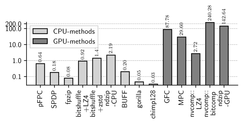
(a) Compression throughputs.

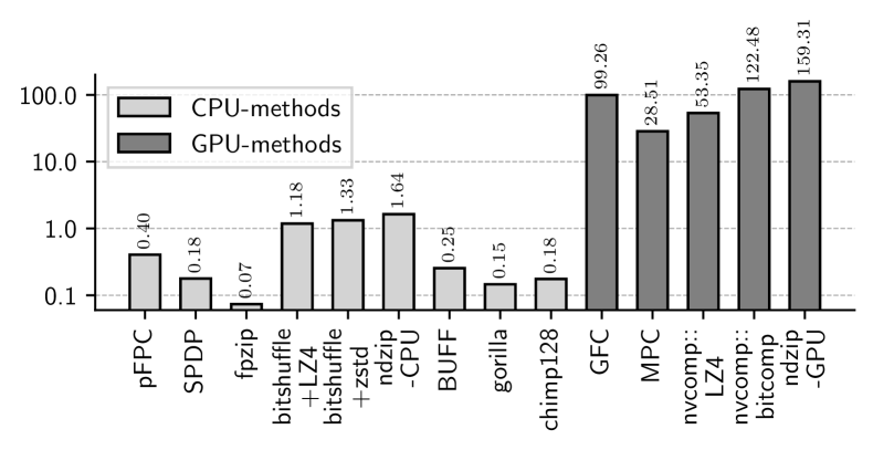
(b) Decompression throughputs.

Figure 8. (De)compression throughputs of different methods.

6.1.3. Decompression Throughput

Not surprisingly, Figure 7(b) shows that GPU-based methods have higher decompression throughput. A bit more interesting observation is shown in Figure 9 that decompression is faster than compression on average. We further observe that (1) ndzip-GPU and ndzip-CPU are the fastest GPU- and CPU-based method respectively, while fpzip has the lowest DT ($0.07$ GB/s). (2) Dictionary-based methods have higher decompression speed than their compression. For nvCOMP::LZ4 and Chimp128, DT are 18.64$\times$ and 4$\times$ of their CT. However, bitshuffle+zstd and bitshuffle::LZ4 have balanced CT and DT. (3) Delta and Lorenzo based methods have balanced compression and decompression speed.

Analysis: (1) Dictionary-based methods require significantly fewer computations during decoding, leading to LZ4 algorithm and Chim128 exhibiting higher decompression times (DT) than compression times (CT). (2) In contrast, delta and Lorenzo predictors perform more balanced operations for both compression and decompression. (3) bitshuffle::zstd and bitshuffle::LZ4 demonstrate balanced CT/DT, behaving more similarly to delta and Lorenzo-based methods. We will later show that they are memory-bound using the roofline model.

Takeaway: Dictionary-based methods do not cause many branch divergences during decompression. Their faster decompression speed is advantageous for query operations, as databases often decompress data multiple times.

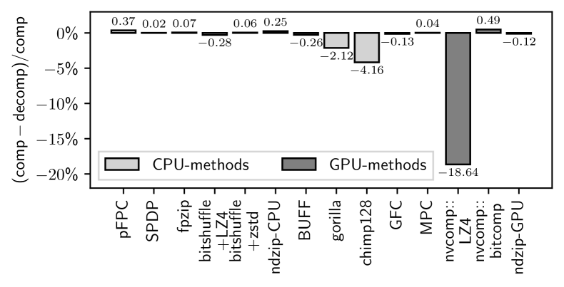
Figure 9. $r_{D}=\frac{CT-DT}{CT}$. Positive $r_{D}$ means compression is faster.

6.1.4. End-to-End Wall Time

Table 6.1.1 shows the wall time of the selected methods and includes the overhead of memory copy from hosts to GPU cards. In terms of end-to-end time, bitshuffle::LZ4 and bitshuffle::zstd are comparable with GFC and MPC, while ndzip-CPU is even faster than ndzip-GPU.

Takeaway: The overhead of host-to-device memory copy is nonnegligible. Bitshuffle::zstd has the best overall computation time plus its highest averaged CR in §6.1.1.

6.1.5. Effect of Dimension Information

Delta and Lorenzo-based methods require dimension information to improve prediction accuracy. In column-based databases, high-dimensional data are stored as 1-d columns. We try to compress the multi-dimensional datasets as 1-d arrays and employ Mann-Whitney U Test (Nachar et al., 2008) ($\alpha=0.05$) to test significant change of CRs. Table 6.1.6 compares the CRs with/without the dimension information. The Mann-Whitney U Test finds no significant difference.

Analysis: (1) Treating high-dimensional data as 1-D arrays causes the Lorenzo predictor to degrade to the delta predictor, which is capable of exposing data correlations. With the aid of bit-level transpose operations, the compression ratios (CRs) of MPC, ndzip-CPU, and ndzip-GPU do not exhibit significant changes. (2) The GFC predictor remains inaccurate, even with the correct dimension information because the residuals are computed from the current chunk and the last value in the previous chunk.

Takeaway: Column-based databases can effectively utilize delta- and Lorenzo-based compression methods as they scale the prediction errors uniformly. Additionally, a bit-level transpose operation can further reduce the impact of these prediction errors.

thread #	pFPC	Bitshfl+LZ4	Bitshfl+Zstd	ndzip-CPU
1
2
4
8
16
24
32
48

Table 7. Parallel compression throughputs.

thread #	pFPC	Bitshfl+LZ4	Bitshfl+Zstd	ndzip-CPU
1
2
4
8
16
24
32
48

Table 8. Parallel decompression throughputs.

6.1.6. Scalability of Parallel Compression

color=blue!40]R4 W2 We measure the scalability of the compressors that support parallel/multi-thread mode, noting that a data parallel design can effectively scale up with multiple threads. Table-8 shows that they can achieve 3$\sim$4$\times$ speedup with 16 to 24 threads compared to their single-thread performances. However, ndzip-CPU does not exhibit similar scalability, which may be due to its implementation issue.

Table 9. Dimension information’s influence on compression ratios.

											GFC	MPC	fpzip	ndzip-C	ndzip-G
	md	1d	md	1d	md	1d	md	1d	md	1d
harmonic mean	1.091	1.089	1.347	1.365	1.334	1.326	1.223	1.210	1.207	1.200
$p$-value ($\alpha=0.05$)	0.957		0.691		0.952		0.848		0.910

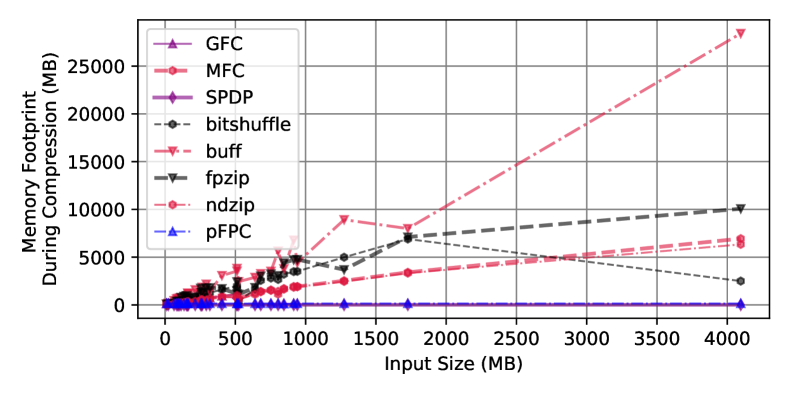
Figure 10. Memory footprints with different input data sizes.

6.1.7. Memory Footprint

color=blue!40]

W2 As shown in Figure 10, while most of the selected compressors use a memory footprint approximately twice the size of the input data, pFPC and SPDP have fixed sizes for their read and write buffers, resulting in a constant memory footprint across all datasets. In contrast, BUFF incurs a memory footprint that is 7$\times$ larger than the input data, rendering it less suitable for in-situ analysis.

6.2. Performance under Context of Databases

Following the micro-benchmarking approach in §5.1.2, we investigate the performance of selected compression methods with different block/chunk sizes in a simulated database system. The compressed data are initially stored in HDF5 files. They are read from the disk and decompressed into Pandas dataframes. Finally, we perform a table scan query.

6.2.1. Performance under Different Block Sizes

Table 10. Compression performance under different block sizes.

blocksize	metrics	pFPC	SPDP	shf+LZ4	shf+zstd	Gorilla	Chimp	nv::LZ4	nv::btcmp
4K	avg-CR	1.151	1.215	1.426	1.463	1.116	1.309	1.244	1.075
	avg-CT (GB/s)	0.018	0.142	1.342	1.271	0.092	0.081	4.953	108.983
	avg-DT (GB/s)	0.017	0.143	1.179	1.190	0.192	0.226	88.669	71.286
64K	avg-CR	1.156	1.239	1.430	1.466	1.095	1.315	1.296	1.094
	avg-CT (GB/s)	0.199	0.254	2.734	2.505	0.120	0.090	2.716	240.280
	avg-DT (GB/s)	0.129	0.250	2.849	3.463	0.332	0.260	53.352	122.483
8M	avg-CR	1.154	1.256	1.361	1.491	1.086	1.315	1.226	1.057
	avg-CT (GB/s)	0.640	0.181	1.384	1.807	0.158	0.104	10.402	68.033
	avg-DT (GB/s)	0.405	0.178	4.467	4.271	0.452	0.294	94.400	50.279

HDF5 datasets consist of multiple disk pages (chunks) (SQLite, 2023) similar to database page files. The default page size ranges from $4$KB to $8$KB. Note that compression algorithms utilizes larger block sizes from $64$KB to $8$MB.

Table 10 displays the average CR, CT, DT of 8 compression algorithms with $4$KB, $64$KB, and $8$MB as block sizes. The best combinations of (method, metric) are highlighted in bold. Seven out of eight compression algorithms yield improved CRs, and all algorithms exhibit higher throughts with $64$KB- and $8$MB- block sizes.

Takeaway: We suggest database designers to increase the default page sizes to improve the compression performances.

6.2.2. Query Performance on TPC Datasets

Table 11. Read and query time (in ms) from HDF5 files.

name

pFPC

SPDP

fpzip

shf+LZ4

shf+zstd

ndzip-C

Gorilla

Chimp

GFC

MPC

ndzip-G

query

tpcH-order

78+ 356

85+ 622

74+ 1577

66+ 94

66+ 72

74+ 60

75+1271

58+ 837

73+ 80

71+ 84

75+1232

190

tpcxBB-store

423+2032

491+3476

423+10162

311+657

299+623

463+712

472+5730

204+4531

-

430+549

462+2024

268

tpcxBB-web

549+2522

612+4643

539+12845

387+777

378+778

597+892

612+8799

266+5748

-

556+685

597+2224

292

tpcH-lineitem

565+2447

640+7463

525+14649

426+758

378+808

579+864

593+3102

339+6153

-

576+669

576+2196

885

tpcDS-catalog

109+ 499

121+1145

100+ 2910

96+135

97+149

106+168

110+1329

105+1131

108+115

103+119

108+1372

64

tpcDS-store

161+ 757

188+1735

150+ 4686

147+217

142+204

161+260

162+1558

151+1769

160+185

156+191

158+1405

106

tpcDS-web

65+ 272

67+ 580

60+ 1457

-

-

60+ 98

64+ 676

61+ 568

63+ 58

62+ 68

58+1231

43

arithmetic mean

1548

3162

7165

679

666

727

3508

3131

211

616

1960

264

To investigate query performance, we measure the running time of three primitive operations depicted in Figure 4: (1) file I/O time to retrieved compressed data from HDF5 files (Folk et al., 2011); (2) data decoding time; (3) full table scan query on the Pandas dataframes (Snider and Swedo, 2004). Table 6.2.2 presents the average reading and query time for selected compression algorithms on the TPC benchmark datasets. For each TPC dataset, the reading overhead varies due to different CRs and DTs based on the compression algorithms; while the query time remains consistent, as the retrieved Pandas dataframes are identical across all algorithms. For instance, pFPC spends $78$ ms to read the compressed chunks and $356$ ms to decompress the TPCH-order data. Subsequently, Pandas uses $190$ ms to query the dataframe.

The query performance aligns with the end-to-end wall time of each method. Despite of its fast query speed, we do not recommend GFC because of its limitation on input data sizes.

Takeaway: We highlight bitshuffle+zstd as the prime CPU-based compressor and MPC as the foremost GPU-based compressor.

6.3. Performance Analysis via Roofline Model

In this section, we examine the the runtime bottlenecks from the standpoint of compression developers. The roofline model (Williams et al., 2009) visualizes algorithms as dots under the roof, which is formed by the peak memory bandwidth and computations.

Figure 10(a) and 10(b) shows the performance of CPU- and GPU-based methods respectively. Each dot represents the most expensive function/loop that consumes greater than $40\%$ computation time of the corresponding methods. We further observe that (1) Most GPU-based methods are close to the memory bandwidth roof. (2) Some CPU-based methods are far below the roof.

Analysis: (1) Serial methods (BUFF, fpzip, SPDP) are not bound by memory or computation. The introduction of parallel techniques could potentially improve their throughputs. (2) The throughput of bitshuffle::LZ4 and bitshuffle::zstd could be enhanced by increasing the number of threads, as evidenced by the scalability test. (3) ndzip::CPU and ndzip::GPU are computation bound. Potential improvements should consider reducing branch divergence.

Takeaway: The roofline model is an effective tool for providing performance insights into the selected algorithms. For instance, it suggests that the throughputs of bitshuffle methods can be improved by utilizing more threads, circumventing the need for costly scalability tests.

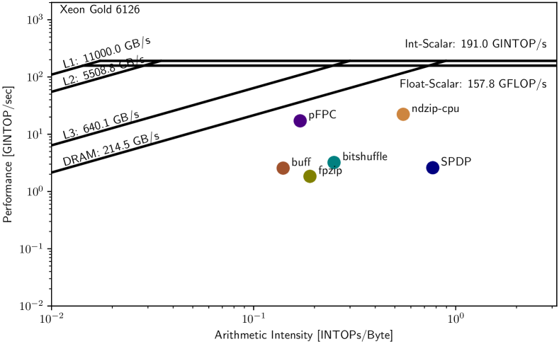
(a) CPU-based methods

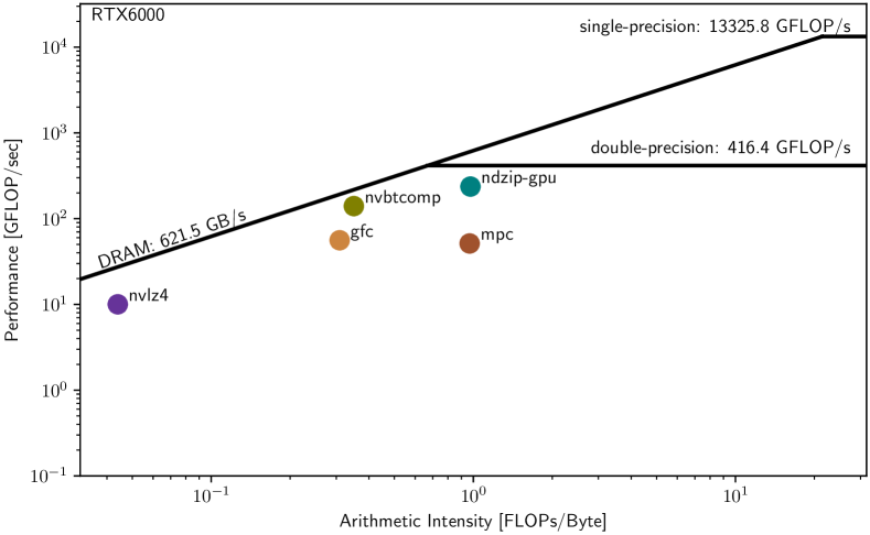
(b) GPU-based methods

Figure 11. Roofline analysis for different methods.

7. Summary

color=blue!40]

W4 In this section, we share the valuable insights from our study. We reflect on key lessons learned, highlight essential takeaways, and conclude with specific recommendations based on our evaluations.

7.1. Lessons Learned

First, understanding the characteristics of data is crucial as it allows us to use single-precision values to achieve higher compression ratios when feasible. Second, while GPU-based methods offer faster computation, the overheads associated with host-to-device data movement and branch divergence often become the bottlenecks.

7.2. Key Takeaways

color=blue!40]R3 W1 For compressor developers: color=blue!40]R1 W1color=blue!40]R3 W3The trade-off between ratio and throughput remains a crucial consideration. When data exhibit a structural layout, such as in scientific simulations and observational data, delta and Lorenzo-based predictors are effective in compression ratios and can easily employ data parallel designs. Conversely, when data display repeated patterns, such as in time series data and database transactions, dictionary-based methods are more effective, albeit at the cost of challenging GPU parallelism due to branch divergence. Ultimately, data transforms like bit and byte-level shuffling effectively improve compression ratios.

For database designers: Compression methods show promise in reducing disk storage, as many algorithms offer fast decompression speeds and can compress 1-D arrays for column-based databases without degrading compression ratio performance. To fully utilize these compression algorithms, it is advisable to set larger default database page sizes.

For system architects: Using the roofline model can reveal that increasing the number of threads and employing parallel computations can improve compression/decompression speeds without the need for expensive scalability tests.

7.3. Recommendations

For users focused on storage reduction: based on the rankings in §6.1.1, we recommend fpzip for HPC data, nvCOMP::LZ4 for time series data, bitshuffle::zstd for observational data, and Chimp for database data. For users needing fast speed: We suggest bitshuffle::LZ4, bitshuffle::zstd, MPC, and ndzip-CPU/GPU, as they demonstrate short end-to-end times in §6.1.4. For general users: We recommend bitshuffle::zstd and MPC due to their balanced performance in average compression ratio (CR), swift end-to-end wall time, and minimal retrieval overhead for queries. Overall, bitshuffle methods rank as the top choice due to their better robustness and lower cost of CPU hardware. .

8. Conclusion

In this study, we conducted a comprehensive examination of 13 lossless floating-point data compressors across 33 datasets from multiple domains. Our analysis delves into their performance, considering not only algorithmic aspects but also architectural considerations. By employing a combination of statistical testing, the roofline model, and a simulated in-memory database, we scrutinized the key designs of the selected compressors. Building on this analysis, we offer recommendations for both compressor researchers and database architecture designers. Additionally, we have created a map to assist users in selecting the most suitable compressors based on their specific requirements. These efforts represent our commitment to bridging the gap between independently developed compression methods in the HPC and database communities.

- (1)
- Lev (2011) 2011. Google LevelDB. https://opensource.googleblog.com/2011/07/leveldb-fast-persistent-key-value-store.html Online.
- hdf (2023) 2023. HDF5 Filters. https://docs.hdfgroup.org/hdf5/develop/_h5_d__u_g.html#subsubsec_dataset_transfer_filter Online.
- rus (2023) 2023. rust-lang. https://www.rust-lang.org/ Online.
- Bellard (2021) Fabrice Bellard. 2021. NNCP v2: Lossless Data Compression with Transformer. (2021).
- Blelloch (2001) Guy E Blelloch. 2001. Introduction to data compression. Computer Science Department, Carnegie Mellon University (2001), 54.
- Boral and Dewitt (1984) Haran Boral and David J Dewitt. 1984. A methodology for database system performance evaluation. ACM SIGMOD Record 14, 2 (1984), 176–185.
- Bugden and Alahmar (2022) William Bugden and Ayman Alahmar. 2022. Rust: The programming language for safety and performance. arXiv preprint arXiv:2206.05503 (2022).
- BURTSCHER (2009) MARTIN BURTSCHER. 2009. Scientific IEEE 754 32-Bit Double-Precision Floating-Point Datasets. https://userweb.cs.txstate.edu/~burtscher/research/datasets/FPdouble/ Online.
- Burtscher and Ratanaworabhan (2007) Martin Burtscher and Paruj Ratanaworabhan. 2007. High throughput compression of double-precision floating-point data. Data Compression Conference Proceedings (2007), 293–302. https://doi.org/10.1109/DCC.2007.44
- Burtscher and Ratanaworabhan (2009) Martin Burtscher and Paruj Ratanaworabhan. 2009. pFPC: A parallel compressor for floating-point data. Data Compression Conference Proceedings (2009), 43–52.
- Cayoglu et al. (2019) Ugur Cayoglu, Frank Tristram, Jörg Meyer, Jennifer Schröter, Tobias Kerzenmacher, Peter Braesicke, and Achim Streit. 2019. Data Encoding in Lossless Prediction-Based Compression Algorithms. In 2019 15th International Conference on eScience (eScience). IEEE, 226–234.
- Claggett et al. (2018) Steven Claggett, Sahar Azimi, and Martin Burtscher. 2018. SPDP: An automatically synthesized lossless compression algorithm for floating-point data. Data Compression Conference Proceedings 2018-March (2018), 335–344. https://doi.org/10.1109/DCC.2018.00042
- Council (2005) Transaction Processing Performance Council. 2005. Transaction processing performance council. Web Site, http://www. tpc. org (2005).
- Demšar (2006) Janez Demšar. 2006. Statistical comparisons of classifiers over multiple data sets. The Journal of Machine learning research 7 (2006), 1–30.
- Du and Ye (2009) Bing Du and ZhongFu Ye. 2009. A novel method of lossless compression for 2-D astronomical spectra images. Experimental Astronomy 27 (2009), 19–26.
- Folk et al. (2011) Mike Folk, Gerd Heber, Quincey Koziol, Elena Pourmal, and Dana Robinson. 2011. An overview of the HDF5 technology suite and its applications. In Proceedings of the EDBT/ICDT 2011 workshop on array databases. 36–47.
- Fonollosa et al. (2015) Jordi Fonollosa, Sadique Sheik, Ramón Huerta, and Santiago Marco. 2015. Reservoir computing compensates slow response of chemosensor arrays exposed to fast varying gas concentrations in continuous monitoring. Sensors and Actuators B: Chemical 215 (2015), 618–629.
- Fout and Ma (2012) Nathaniel Fout and Kwan-Liu Ma. 2012. An adaptive prediction-based approach to lossless compression of floating-point volume data. IEEE Transactions on Visualization and Computer Graphics 18, 12 (2012), 2295–2304.
- Freeman et al. (2021) Cynthia Freeman, Jonathan Merriman, Ian Beaver, and Abdullah Mueen. 2021. Experimental Comparison and Survey of Twelve Time Series Anomaly Detection Algorithms. Journal of Artificial Intelligence Research 72 (2021), 849–899.
- Goldberg (1991) David Goldberg. 1991. What every computer scientist should know about floating-point arithmetic. ACM computing surveys (CSUR) 23, 1 (1991), 5–48.
- Goyal et al. (2021) Mohit Goyal, Kedar Tatwawadi, Shubham Chandak, and Idoia Ochoa. 2021. DZip: Improved general-purpose loss less compression based on novel neural network modeling. Data Compression Conference Proceedings 2021-March (2021), 153–162. Issue Dcc. https://doi.org/10.1109/DCC50243.2021.00023
- Grosset and Ahrens (2021) Pascal Grosset and James Ahrens. 2021. Lightweight Interface for In Situ Analysis and Visualization of Particle Data. In ISAV’21: In Situ Infrastructures for Enabling Extreme-Scale Analysis and Visualization. 12–17.
- Habib et al. (2016) Salman Habib, Adrian Pope, Hal Finkel, Nicholas Frontiere, Katrin Heitmann, David Daniel, Patricia Fasel, Vitali Morozov, George Zagaris, Tom Peterka, et al. 2016. HACC: Simulating sky surveys on state-of-the-art supercomputing architectures. New Astronomy 42 (2016), 49–65.
- Haven (2018) Poly Haven. 2018. HDRIs / Preller Drive. https://hdrihaven.com/hdri/?c=night&h=preller_drive Online.
- Haven (2020) Poly Haven. 2020. HDRIs / Palermo Sidewalk. https://polyhaven.com/a/palermo_sidewalk Online.
- Holder et al. (2023) Christopher Holder, Matthew Middlehurst, and Anthony Bagnall. 2023. A review and evaluation of elastic distance functions for time series clustering. Knowledge and Information Systems (2023), 1–45.
- Huber et al. (2021) David Huber, Ralf Kissmann, and Olaf Reimer. 2021. Relativistic fluid modelling of gamma-ray binaries-II. Application to LS 5039. Astronomy & Astrophysics 649 (2021), A71.
- Ibarria et al. (2003) Lawrence Ibarria, Peter Lindstrom, Jarek Rossignac, and Andrzej Szymczak. 2003. Out-of-core compression and decompression of large n-dimensional scalar fields. In Computer Graphics Forum, Vol. 22. Wiley Online Library, 343–348.
- Intel (2023) Intel. 2023. Intel® Advisor. https://www.intel.com/content/www/us/en/developer/tools/oneapi/advisor.html Online.
- IRSA (2023) IRSA. 2023. Spitzer Documentation & Tools. https://irsa.ipac.caltech.edu/data/SPITZER/FLS/images/irac/ Online.
- Kaggle (2019) Kaggle. 2019. Climate Weather Surface of Brazil - Hourly — kaggle.com. https://www.kaggle.com/datasets/PROPPG-PPG/hourly-weather-surface-brazil-southeast-region Online.
- Kaggle (2021) Kaggle. 2021. NYC Yellow Taxi Trip Data — kaggle.com. https://www.kaggle.com/datasets/elemento/nyc-yellow-taxi-trip-data Online.
- Kaggle (2022a) Kaggle. 2022a. Daily Prices for Spanish Gas Stations (2007-2022) — kaggle.com. https://www.kaggle.com/datasets/mauriciy/daily-spanish-gas-prices Online.
- Kaggle (2022b) Kaggle. 2022b. Jane Street Market Prediction — kaggle.com. https://www.kaggle.com/competitions/jane-street-market-prediction/data Online.
- Kaggle (2022c) Kaggle. 2022c. MagNet NASA Dataset — kaggle.com. https://www.kaggle.com/datasets/kingabzpro/magnet-nasa?select=solar_wind.csv Online.
- Kahan (1996) William Kahan. 1996. IEEE standard 754 for binary floating-point arithmetic. Lecture Notes on the Status of IEEE 754, 94720-1776 (1996), 11.
- Keahey et al. (2020) Kate Keahey, Jason Anderson, Zhuo Zhen, Pierre Riteau, Paul Ruth, Dan Stanzione, Mert Cevik, Jacob Colleran, Haryadi S. Gunawi, Cody Hammock, Joe Mambretti, Alexander Barnes, François Halbach, Alex Rocha, and Joe Stubbs. 2020. Lessons Learned from the Chameleon Testbed. In Proceedings of the 2020 USENIX Annual Technical Conference (USENIX ATC ’20). USENIX Association.
- Kissmann et al. (2016) R Kissmann, K Reitberger, O Reimer, A Reimer, and E Grimaldo. 2016. Colliding-wind binaries with strong magnetic fields. The Astrophysical Journal 831, 2 (2016), 121.
- Klacansky (2009) Pavol Klacansky. 2009. open-scivis-datasets. https://klacansky.com/open-scivis-datasets/ Online.
- Knoll (2023) Byron Knoll. 2023. CMIX. https://github.com/byronknoll/cmix Online.
- Knorr et al. (2020) Fabian Knorr, Peter Thoman, and Thomas Fahringer. 2020. Datasets for Benchmarking Floating-Point Compressors. arXiv preprint arXiv:2011.02849 (2020).
- Knorr et al. (2021a) Fabian Knorr, Peter Thoman, and Thomas Fahringer. 2021a. Ndzip: A High-Throughput Parallel Lossless Compressor for Scientific Data. Data Compression Conference Proceedings 2021-March, 103–112. https://doi.org/10.1109/DCC50243.2021.00018
- Knorr et al. (2021b) Fabian Knorr, Peter Thoman, and Thomas Fahringer. 2021b. ndzip-gpu: efficient lossless compression of scientific floating-point data on GPUs. In Proceedings of the International Conference for High Performance Computing, Networking, Storage and Analysis. 1–14.
- Liakos et al. (2022) Panagiotis Liakos, Katia Papakonstantinopoulou, and Yannis Kotidis. 2022. Chimp: efficient lossless floating point compression for time series databases. Proceedings of the VLDB Endowment 15, 11 (2022), 3058–3070.
- Lindstrom (2017) Peter Lindstrom. 2017. Error distributions of lossy floating-point compressors. Technical Report. Lawrence Livermore National Lab.(LLNL), Livermore, CA (United States).
- Lindstrom and Isenburg (2006) Peter Lindstrom and Martin Isenburg. 2006. fpzip-Fast and efficient compression of floating-point data. IEEE Transactions on Visualization and Computer Graphics 12 (2006), 1245–1250. Issue 5. https://doi.org/10.1109/TVCG.2006.143
- Lissandrini et al. (2018) Matteo Lissandrini, Martin Brugnara, and Yannis Velegrakis. 2018. Beyond macrobenchmarks: microbenchmark-based graph database evaluation. Proceedings of the VLDB Endowment 12, 4 (2018), 390–403.
- Liu et al. (2021) Chunwei Liu, Hao Jiang, John Paparrizos, and Aaron J. Elmore. 2021. BUFF: Decomposed bounded floats for fast compression and queries. Proceedings of the VLDB Endowment 14 (2021), 2586–2598. Issue 11. https://doi.org/10.14778/3476249.3476305
- Martin (1979) G Nigel N Martin. 1979. Range encoding: an algorithm for removing redundancy from a digitised message. In Proc. Institution of Electronic and Radio Engineers International Conference on Video and Data Recording, Vol. 2.
- MAST (2023) MAST. 2023. MAST: Barbara A. Mikulski Archive for Space Telescopes. https://mast.stsci.edu/portal/Mashup/Clients/Mast/Portal.html Online.
- Masui et al. (2015) K. Masui, M. Amiri, L. Connor, M. Deng, M. Fandino, C. Höfer, M. Halpern, D. Hanna, A. D. Hincks, G. Hinshaw, J. M. Parra, L. B. Newburgh, J. R. Shaw, and K. Vanderlinde. 2015. A compression scheme for radio data in high performance computing. Astronomy and Computing 12 (2015), 181–190. https://doi.org/10.1016/j.ascom.2015.07.002
- Nachar et al. (2008) Nadim Nachar et al. 2008. The Mann-Whitney U: A test for assessing whether two independent samples come from the same distribution. Tutorials in quantitative Methods for Psychology 4, 1 (2008), 13–20.
- NVIDIA (2023) NVIDIA. 2023. nvCOMP. https://github.com/NVIDIA/nvcomp Online.
- Nvidia (2023) Nvidia. 2023. NVIDIA Nsight Compute. https://developer.nvidia.com/nsight-compute Online.
- O’Neil and Burtscher (2011) Molly A O’Neil and Martin Burtscher. 2011. Floating-point data compression at 75 Gb/s on a GPU. In Proceedings of the Fourth Workshop on General Purpose Processing on Graphics Processing Units. 1–7.
- Oseret and Timsit (2007) Emmanuel Oseret and Claude Timsit. 2007. Optimization of a lossless object-based compression embedded on GAIA, a next-generation space telescope. In Mathematics of Data/Image Pattern Recognition, Compression, Coding, and Encryption X, with Applications, Vol. 6700. SPIE, 24–35.
- Pelkonen et al. (2015) Tuomas Pelkonen, Scott Franklin, Justin Teller, Paul Cavallaro, Qi Huang, Justin Meza, and Kaushik Veeraraghavan. 2015. Gorilla: A fast, scalable, in-memory time series database. Proceedings of the VLDB Endowment 8 (2015), 1816–1827. Issue 12. https://doi.org/10.14778/2824032.2824078
- Ross et al. (2020) Robert B Ross, George Amvrosiadis, Philip Carns, Charles D Cranor, Matthieu Dorier, Kevin Harms, Greg Ganger, Garth Gibson, Samuel K Gutierrez, Robert Latham, et al. 2020. Mochi: Composing data services for high-performance computing environments. Journal of Computer Science and Technology 35, 1 (2020), 121–144.
- Roth and Van Horn (1993) Mark A Roth and Scott J Van Horn. 1993. Database compression. ACM Sigmod Record 22, 3 (1993), 31–39.
- Rubio-González et al. (2013) Cindy Rubio-González, Cuong Nguyen, Hong Diep Nguyen, James Demmel, William Kahan, Koushik Sen, David H Bailey, Costin Iancu, and David Hough. 2013. Precimonious: Tuning assistant for floating-point precision. In Proceedings of the international conference on high performance computing, networking, storage and analysis. 1–12.
- Saeedan and Eldawy (2022) Majid Saeedan and Ahmed Eldawy. 2022. Spatial parquet: a column file format for geospatial data lakes. In Proceedings of the 30th International Conference on Advances in Geographic Information Systems. 1–4.
- Sayood (2017) Khalid Sayood. 2017. Introduction to data compression. Morgan Kaufmann.
- Schmidt et al. (2018) Philip Schmidt, Attila Reiss, Robert Duerichen, Claus Marberger, and Kristof Van Laerhoven. 2018. Introducing wesad, a multimodal dataset for wearable stress and affect detection. In Proceedings of the 20th ACM international conference on multimodal interaction. 400–408.
- Snider and Swedo (2004) LA Snider and SE Swedo. 2004. PANDAS: current status and directions for research. Molecular psychiatry 9, 10 (2004), 900–907.
- Son et al. (2014) Seung Woo Son, Zhengzhang Chen, William Hendrix, Ankit Agrawal, Wei-keng Liao, and Alok Choudhary. 2014. Data compression for the exascale computing era-survey. Supercomputing frontiers and innovations 1, 2 (2014), 76–88.
- SQLite (2023) SQLite. 2023. The Default Page Size Change of SQLite 3.12.0. https://www.sqlite.org/pgszchng2016.html Online.
- Stisen et al. (2015) Allan Stisen, Henrik Blunck, Sourav Bhattacharya, Thor Siiger Prentow, Mikkel Baun Kjærgaard, Anind Dey, Tobias Sonne, and Mads Møller Jensen. 2015. Smart devices are different: Assessing and mitigatingmobile sensing heterogeneities for activity recognition. In Proceedings of the 13th ACM conference on embedded networked sensor systems. 127–140.
- Stockman (1999) HS Stockman. 1999. Data compression for the next-generation space telescope. In Proceedings DCC’99 Data Compression Conference (Cat. No. PR00096). IEEE, 542.
- Thoman et al. (2019) Peter Thoman, Philip Salzmann, Biagio Cosenza, and Thomas Fahringer. 2019. Celerity: High-level c++ for accelerator clusters. In Euro-Par 2019: Parallel Processing: 25th International Conference on Parallel and Distributed Computing, Göttingen, Germany, August 26–30, 2019, Proceedings 25. Springer, 291–303.
- Thoman et al. (2020) Peter Thoman, Markus Wippler, Robert Hranitzky, and Thomas Fahringer. 2020. RTX-RSim: Accelerated Vulkan room response simulation for time-of-flight imaging. In Proceedings of the International Workshop on OpenCL. 1–11.
- TPC (2023a) TPC. 2023a. TPC-DS Vesion 2 and Version 3. https://www.tpc.org/tpcds/default5.asp Online.
- TPC (2023b) TPC. 2023b. TPC-H Vesion 2 and Version 3. https://www.tpc.org/tpch/ Online.
- TPC (2023c) TPC. 2023c. TPCx-BB. https://www.tpc.org/tpcx-bb/default5.asp Online.
- Wang et al. (2017) Jianguo Wang, Chunbin Lin, Yannis Papakonstantinou, and Steven Swanson. 2017. An experimental study of bitmap compression vs. inverted list compression. In Proceedings of the 2017 ACM International Conference on Management of Data. 993–1008.
- Williams et al. (2009) Samuel Williams, Andrew Waterman, and David Patterson. 2009. Roofline: an insightful visual performance model for multicore architectures. Commun. ACM 52, 4 (2009), 65–76.
- Yang et al. (2015) Annie Yang, Hari Mukka, Farbod Hesaaraki, and Martin Burtscher. 2015. MPC: a massively parallel compression algorithm for scientific data. In 2015 IEEE International Conference on Cluster Computing. IEEE, 381–389.
- Zhao et al. (2020) Kai Zhao, Sheng Di, Xin Lian, Sihuan Li, Dingwen Tao, Julie Bessac, Zizhong Chen, and Franck Cappello. 2020. SDRBench: Scientific data reduction benchmark for lossy compressors. In 2020 IEEE International Conference on Big Data (Big Data). IEEE, 2716–2724.
- Ziv and Lempel (1977) Jacob Ziv and Abraham Lempel. 1977. A universal algorithm for sequential data compression. IEEE Transactions on information theory 23, 3 (1977), 337–343.