On a Generalization of Wasserstein Distance and the Beckmann Problem to Connection Graphs

Abstract.

The intersection of connection graphs and discrete optimal transport presents a novel paradigm for understanding complex graphs and node interactions. In this paper, we delve into this unexplored territory by focusing on the Beckmann problem within the context of connection graphs. Our study establishes feasibility conditions for the resulting convex optimization problem on connection graphs. Furthermore, we establish strong duality for the conventional Beckmann problem, and extend our analysis to encompass strong duality and duality correspondence for a quadratically regularized variant. To put our findings into practice, we implement the regularized problem using gradient descent, enabling a practical approach to solving this complex problem. We showcase optimal flows and solutions, providing valuable insights into the real-world implications of our theoretical framework.

1. Introduction and Related Work

Optimal transport involves defining and computing measures of discrepancy between probability distributions. These measures represent the cost of moving mass between distribution-modeled locations. Historically, optimal transport of probability measures started with the Monge formulation in 1781 [27] and later evolved to include the Kantorovich relaxation [21]. In recent times, the field of optimal transport has attracted considerable attention from computational researchers [30] for its wide variety of applications; including transportation network design [26], community detection [14, 23], supervised and unsupervised learning on point cloud valued data [28, 22, 12], and image processing and computer vision [29, 5] to name a few.

The subfield of discrete optimal transport [35, 18] pertains to the class of problems that involve discrete probability measures or transport between measures defined on discrete spaces. These problems have garnered particular interest due to their prevalence in the implementation of the various optimal transport problems and applications. The Beckmann problem, focusing on optimal transport between densities on graphs [30], leverages insights from geometric and dynamic optimal transport frameworks [32]. In turn, without directly dealing with the shortest path distances between all node pairs, the aforementioned approach capitalizes on the often sparse edge structure of a graph to enhance the scalability and manage the complexity of calculating the Wasserstein distance, i.e., the cost of optimal transport, as explained in [35].

In this paper we generalize the Beckmann problem to a class of graphs known as connection graphs, which can be understood in this case as undirected and weighted graphs equipped with a rotation structure on each edge. This class of graphs has received interest in recent years for a variety of applications, including angular synchronization problems [33], Cheeger constants [1], graph effective resistance and random walks [13], graph embedding algorithms [34], cryo-electron microscopy [3], graph neural network models [2], and solving jigsaw puzzles [20]. The focus of this paper is a generalization of the Beckmann problem from general graphs to connection graphs, and in turn from scalar to vector-valued probability densities defined on graphs. In fact, a $1$d connection graph with trivial signatures is just an undirected graph for which the Beckmann problem is already defined [35].

One of the key contributions of this paper is the guarantee that any connection graph is switching equivalent to another graph on which the Beckmann problem is always feasible (Theorem 2.3). It is worthwhile to highlight the fact that the proof of this result relies heavily on balance theory, which can be informally described as the study of how various properties and aspects of a connection graph depend and relate to how well-synchronized the rotations on the graph are. Balance theory has been studied in several contexts (e.g. [38], [7]). Therefore this paper represents a new and interesting facet of the balance theory of connection graphs.

Transport phenomena involving vector-valued densities on connection graphs have versatile applications, as exemplified by three scenarios. First, as established by Singer and Wu [34], when the nodes of graph $G$ are positioned on or near a $d$-dimensional Riemannian manifold within $\mathbb{R}^{n}$, the connection Laplacian can effectively model interactions occurring on the tangent bundle of this manifold. This implies that transport within the connection graph $G$ offers a discrete approach to simulating vector-valued mass transport on the tangent bundle of a Riemannian manifold. Secondly, building on insights from Lieb and Loss [24], if the nodes of the graph $G$ are situated within a magnetic field environment, the connectivity structure of the edges can be harnessed to represent rotational flux between two specific points. In this context, mass transport within the connection graph can be interpreted as the movement of mass influenced by rotational forces. Lastly, as introduced by Ryu et al. [31], when the nodes of the graph $G$ correspond to pixels in an image, irrespective of whether there is additional connection or rotation structure, vector-valued densities offer a potent tool for image modeling. Consequently, evaluating the transport cost between these densities can provide insights into what may be termed the color Earth mover’s distance [37] for understanding differences in color distribution in images. These three applications underscore the adaptability of utilizing transport between vector-valued densities on connection graphs for modeling various physical phenomena and systems.

1.1. Summary of Main Results

This paper contains three novel contributions. First, we propose an innovative approach to optimal transport between vector-valued densities on connection graphs, formulated as follows (see Section 1.4 for a detailed discussion):

(1) $$\mathcal{W}_{1}^{\sigma}(\alpha,\beta)=\inf_{J\in\ell_{2}(E^{\prime};\mathbb{R}^{d})}\left\{\sum_{e\in E^{\prime}}w(e)\|J(e)\|_{2}:\operatorname{div}(J)=\alpha-\beta\right\},$$

and we provide a detailed theoretical analysis of its feasibility. This is crucial due to the fact that, unlike conventional graphs, establishing a feasible “flow” $J$ as in Eq. 1 may not be attainable for two vector-valued probability densities. Second, we study the resulting duality theory and establish strong duality for the Beckmann problem on connection graphs. Third, we propose a quadratically regularized version of the problem in a manner similar to Solomon and Essid [35], and provide a detailed analysis of the resulting duality theory—particularly duality correspondence (see Theorem 2.4), which allows one to convert between solutions for the primal and dual versions of the problem. This is particularly helpful in Section 4 by enabling a scalable gradient descent-based approach to calculating the optimal cost and flow between any two densities.

1.2. Organization of this paper

In Section 1.3, we begin by introducing the relevant terminology and graph-theoretic preliminaries needed for our work.

In Section 1.4 we review the discrete optimal transport theory and the Beckmann problem on graphs. Additionally, we present a natural extension of the Beckmann problem to encompass connection graphs.

Then, in Section 2, we examine the feasibility of the problem, derive the Lagrangian dual and establish strong duality. In Section 3 we formulate a strictly convex version of the Beckmann problem by incorporating quadratic regularization and re-establish strong duality. We also elucidate the process of converting a dual problem solution (a potential function on the vertices) to a distinct solution of the primal problem (a flow along the edges). Finally, in Section 4 we solve the quadratically regularized problem in a variety of settings and provide visual intuition of the optimal flow on the underlying graph.

1.3. Graph theory preliminaries

We start by fixing a finite, connected, weighted, and undirected graph $G=(V,E,w)$. Here, for convention we assume $V=\{1,2,\dotsc,n\}$ for some $n\geq 2$, $E\subset{V\choose 2}$, and $|E|=m$ for some $m\geq 1$. The weights $w=(w_{ij})_{i,j\in V}$ are assumed to be symmetric nonnegative real numbers such that $w_{ij}>0$ if and only if $\{i,j\}\in E$. For each $i,j\in V$ we write $i\sim j$ if $\{i,j\}\in E$ and for each vertex $i\in V$ we define its degree:

(2) $$d_{i}=\sum_{j\sim i}w_{ij}.$$

A path is an ordered tuple of adjacent vertices $P=(i_{1},i_{2},\dotsc,i_{n})$ where $i_{\ell}\sim i_{\ell+1}$ for $1\leq\ell\leq n-1$. The length of a path is the number of (possibly non-unique) edges its entries contain. A cycle $C$ is a path where $i_{1}=i_{n}$. If $P$ is a path as before and $Q=(j_{1},j_{2},\dotsc,j_{n})$ is a second path satisfying $i_{n}\sim j_{1}$, then ${P}{Q}$ is defined to be the concatenated path

(3) $${P}{Q}=(i_{1},\dotsc,i_{n},j_{1},\dotsc,j_{n}).$$

Lastly we define $P^{-1}$ to be the path $P$ with reversed orientation, namely $P^{-1}=(i_{n},i_{n-1},\dotsc,i_{1})$.

For a fixed graph $G=(V,E,w)$ we define $E^{\prime}$ to be a canonically oriented edge set, namely

(4) $$E^{\prime}=\{(i,j):i<j,i\sim j\}.$$

The choice of orientation/enumeration used to construct $E^{\prime}$ has no impact on the subsequent results. This is done solely to have consistent definitions for incidence matrices and their induced operators.

For $d\geq 1$, the notation $\mathbb{O}(d)$ refers to the group of $d\times d$ orthogonal matrices; i.e., matrices $O\in\mathbb{R}^{d\times d}$ such that $O^{T}O=OO^{T}=I_{d}$.

Definition 1.1.

Let $E^{\prime\prime}=\{(i,j),(j,i):i,j\in V{\hskip 5.69046pt}i\sim j\}$. A connection is a map $\sigma:E^{\prime\prime}\rightarrow\mathbb{O}(d)$ for some $d\geq 1$ satisfying $\sigma((i,j)):=\sigma_{ij}=\sigma_{ji}^{-1}$ for each $(i,j)\in E^{\prime\prime}$. A pair $(G,\sigma)$ is called a connection graph.

Let $(G,\sigma)$ be a fixed connection graph. If $P=(i_{1},\dotsc,i_{n})$ is a path, we define

(5) $$\sigma_{P}=\prod_{\ell=1}^{n-1}\sigma_{i_{\ell},i_{\ell+1}}.$$

It is useful to observe that if $P,Q$ are paths in $G$ then $\sigma_{{P}{Q}}=\sigma_{P}\sigma_{Q}$ and $\sigma_{P^{-1}}=\sigma_{P}^{-1}$.

The connection incidence matrix $B\in\mathbb{R}^{nd\times md}$ is the block matrix defined by

(6) $$B=(B_{ie})_{i\in V,e\in E^{\prime}},{\hskip 5.69046pt}B_{ie}=\begin{cases}\sqrt{w_{e}}I_{d}&\text{ if }e=(i,\cdot)\\ -\sqrt{w_{e}}\sigma_{e}^{T}&\text{ if }e=(\cdot,i)\\ 0&\text{ otherwise}\end{cases}.$$

The connection Laplacian matrix $L\in\mathbb{R}^{nd\times nd}$ is defined by the equation $L=BB^{T}$, or blockwise by the equation

(7) $$L=(L_{ij})_{i,j\in V},{\hskip 5.69046pt}L_{ij}=\begin{cases}d_{i}I_{d}&\text{ if }i=j\\ -w_{ij}\sigma_{ij}&\text{ if }i\sim j\\ 0_{d\times d}&\text{ otherwise}\end{cases}$$

where $L_{ij}\in\mathbb{R}^{d\times d}$ for each $i,j\in V$. If $D=\text{diag}(d_{1},\dotsc,d_{n})$ and $A$ is the adjacency matrix of $G=(V,E)$, then $\Delta=D-A$ is the standard combinatorial Laplacian matrix of $G$. Both $L$ and $\Delta$ are symmetric and positive semi-definite and hence have nonnegative eigenvalues.

We use the notation $\ell_{2}(V;\mathbb{R}^{d})$ to denote the vector space of functions $f:V\rightarrow\mathbb{R}^{d}$, identified with their column vector representations

(8) $$f=\begin{bmatrix}f(1)\\ f(2)\\ \vdots\\ f(n)\end{bmatrix}\in\mathbb{R}^{nd\times 1}$$

and which we equip with the standard real $\ell_{2}$ inner product

(9) $$\langle f,g\rangle=f^{T}g$$

for each $f,g\in\ell_{2}(V;\mathbb{R}^{d})$. We similarly define $\ell_{2}(E^{\prime};\mathbb{R}^{d})$ in the obvious manner.

Definition 1.2.

The (connection) gradient operator $\nabla:\ell_{2}(V;\mathbb{R}^{d})\rightarrow\ell_{2}(E^{\prime};\mathbb{R}^{d})$ is defined by the action of $B^{T}$ on the vector representation of each $f\in\ell_{2}(V;\mathbb{R}^{d})$. Specifically, $\nabla f=B^{T}f$ where, for each $e\in E^{\prime}$,

(10) $$(\nabla f)_{e=(i,j)}=\sqrt{w_{ij}}(f(i)-\sigma_{ij}f(j)).$$

Similarly, the divergence operator $\operatorname{div}:\ell_{2}(E^{\prime};\mathbb{R}^{d})\rightarrow\ell_{2}(V;\mathbb{R}^{d})$ is defined by the action of $B$ on the vector representation of each $J\in\ell_{2}(E^{\prime};\mathbb{R}^{d})$. In particular, $\operatorname{div}J=BJ$ where, for each $i\in V$,

(11) $$(BJ)_{i}=\sum_{j:((i,j))\in E^{\prime}}\sqrt{w_{ij}}J(i,j)-\sum_{j:(j,i)\in E^{\prime}}\sqrt{w_{ji}}\sigma_{ij}J(j,i).$$

There is a natural duality between $\nabla$ and $\operatorname{div}$; i.e., we can write

(12) $$\langle\operatorname{div}J,f\rangle_{V}=\langle J,\nabla f\rangle_{E}.$$

This can be considered an analogue of the Green’s identity for functions on connection graphs.

Definition 1.3.

Let $(G,\sigma)$ be a connection graph. Then $G$ is called balanced if for any cycle $C=(i_{1},i_{2},\dotsc,i_{n},i_{n}=i_{1})$ where $i_{\ell}\sim i_{\ell+1}$ for each $1\leq\ell\leq n-1$, it holds that $\sigma_{C}=I_{d}$.

Definition 1.4.

Let $(G,\sigma)$ be a connection graph. If $\tau:V\rightarrow\mathbb{O}(d)$ is any function, then we define the $\tau$-switched signature $\sigma^{\tau}$ via the equation

(13) $$\sigma^{\tau}_{ij}=\tau(i)^{-1}\sigma_{ij}\tau(j).$$

Definition 1.5.

Two signatures $\rho$ and $\sigma$ on $G$ are called switching equivalent if there exists some $\tau$ for which $\rho=\sigma^{\tau}$.

We recall the following theorem from[9, Theorem 1]:

Theorem 1.1.

Let $(G,\sigma)$ be a connection graph. Then TFAE:

1. $G$ is balanced.

2. $L$ has kernel of dimension $d$; i.e., the multiplicity of the eigenvalue 0 in the spectrum of $L$ is $d$.

3. The eigenvalues of $L$ are exactly the eigenvalues of the combinatorial laplacian matrix $\Delta$ of $G$ each occuring with multiplicity $d$.

4. There exists a map $\tau:V\rightarrow\mathbb{O}(d)$ such that $\tau(i)=\sigma_{ij}\tau(j)$ for each $i,j\in V$.

5. $\sigma$ is switching equivalent to the trivial signature $\iota:(i,j)\mapsto I_{d}$.

1.4. Optimal transport on graphs

In this subsection we review optimal transport cost for probability densities on graphs via the Kantorovich problem. Generally speaking, optimal transport cost can be understood as the minimal amount of work, or cost, required to move a unit of mass in a “pile” modeled by the density $\alpha$ to a “ditch” modeled by a second density $\beta$. Alternatively, Wasserstein distance (a specific optimal transport formulation) can be thought of as the mean $\ell_{p}$ distance between points sampled from densities $\alpha,\beta$ in pairs according to an “optimal” probability distribution on the product $V\times V$ with marginals $\alpha,\beta$.

In this paper we consider two specific formulations: the Kantorovich and Beckmann optimal transport problems where the underlying space is a connection graph and the transportation cost reflects the presence of the signature. The Kantorovich optimal transport problem on a standard graph $G$ can be posed using the shortest path distances $\{d_{ij}\}_{i,j\in V}$, as follows:

(14) $$\mathcal{W}_{1}(\alpha,\beta)=\inf_{U\in\mathbb{R}^{n\times n}}\left\{\sum_{i,j=1}^{n}d_{ij}U_{ij}:U\geq 0,U1_{n}=\alpha,U^{T}1_{n}=\beta\right\}.$$

$\mathcal{W}_{1}(\alpha,\beta)$ is called the 1-Wasserstein metric or the Earth mover’s distance on the space of distributions $\mathcal{P}(G)=\{f\in\ell_{2}(V;\mathbb{R}):f\geq 0,\sum_{i\in V}f(i)=1\}$, and represents the optimal cost for transporting $\alpha$ to $\beta$ on $G$ [30, 17, 25]. The plan(s) $U$ achieving $\mathcal{W}_{1}(\alpha,\beta)$ are called optimal transportation plans and its entries $U_{ij}$, loosely speaking, encode how much mass from node $i$ is moved to node $j$.

Pursuant to work in [19] in the case of probability measures on $\mathbb{R}^{d}$ and detailed in [15] in the case of graphs, an alternative formulation to Eq. 14 based on a dynamic, or flow-based approach can be expressed in the Beckmann formulation of the optimal transport problem:

(15) $$\mathcal{W}_{1}(\alpha,\beta)=\inf_{J\in\ell_{2}(E^{\prime};\mathbb{R})}\left\{\sum_{e\in E^{\prime}}w(e)|J(e)|:\mathrm{div}J=\alpha-\beta\right\}.$$

Here $J$ represents a signed flow along each edge, and the constraint $\operatorname{div}(J)=\alpha-\beta$ ensures that the flow $J$ transports mass from $\alpha$ to $\beta$. The advantage of using this formulation lies in the fact that the graph $G$ inherently captures the local connectivity structure of the underlying metric space. Consequently, a full coupling $U$ contains redundant information, and thus its computation is unnecessary. Mass transport is naturally restricted to occur between adjacent vertices along edges, rather than involving teleportation between distant nodes. As a result, when dealing with a sparse graph $G$, optimizing over the flow $J$ reduces the complexity of the problem compared to the Earth Mover’s Distance equation (Eq. 14).

1.5. Vector-valued optimal transport on connection graphs

In this paper, we shift our focus from working with scalar-valued densities to considering vector-valued densities on the graph $G$. To wit:

Definition 1.6.

A vector-valued probability density on a graph $G$ is a function $\alpha\in\ell_{2}(V;\mathbb{R}^{d})$ which satisfies

1. $\alpha(i)_{\ell}\geq 0$ for each $i\in V$ and $1\leq\ell\leq d$.

2. $\sum_{i\in V}\alpha(i)_{\ell}=1_{d}$, where $1_{d}^{T}=[1,\ldots,1]$.

We use $\mathcal{P}_{d}(G)$ to refer to the set of all vector-valued probability densities on $G$ with target $\mathbb{R}^{d}$.

One of the reasons for this approach is motivated by the manifold setting. Let’s suppose that the graph $G$ is a discretization of a $d$-dimensional Riemannian manifold and let $i,j\in V$ be fixed. In this context, there exist a $d$-dimensional orthonormal basis of the tangent space at $i$. If there is an edge between nodes $i$ and $j$, the connection $\sigma_{ij}$ can be interpreted as an approximation of the parallel transport operator, responsible for transporting vectors from the tangent space at $i$ to the tangent space at $j$ on the manifold.

Under this setting, we interpret the masses $\alpha(i)$ and $\beta(i)$ as vectors residing in the $d$-dimensional orthonormal basis of the tangent spaces. The main objective is to find an optimal flow of masses on the tangent bundle, i.e. across the tangent spaces, which minimizes a cost function that takes into account not only the length of paths between nodes by incorporating weights $w_{ij}$ but also the compatibility of the transformations $\sigma_{ij}$ along these paths. To illustrate, the cost $d_{ij}$ can be seen as the vector diffusion distance, as described in [34]. This approach allows us to consider more complex and informative interactions between vector-valued densities on the graph.

In addition to the geometric perspective, one can also conceptualize vector-valued densities (specifically the case of $d=3$) as taking values in color channels in an image processing setting. Thus, if $G$ is equipped with an embedding that can facilitate image rendering (such is the case naturally if $G$ is a grid graph), transport cost between $\alpha$ and $\beta$ can be understood as a metric or distance function between images.

There have been many inroads investigating the theoretical properties and applications of transport between vector-valued densities in recent years [8, 31, 11]. The formulation we present below, and the subsequent duality result, are based on a recent approach introduced in [10], and the duality for the Beckmann problem discussed in [32, Problem 4.5].

Let $(G,\sigma)$ be a connection graph. We define the connection 1-Wasserstein distance $\mathcal{W}_{1}^{\sigma}(\alpha,\beta)$ for vector-valued measures $\alpha,\beta\in\mathcal{P}_{d}(G)$ by:

(16) $$\mathcal{W}_{1}^{\sigma}(\alpha,\beta)=\inf_{J\in\ell_{2}(E^{\prime};\mathbb{R}^{d})}\left\{\sum_{e\in E^{\prime}}w(e)\|J(e)\|_{2}:\operatorname{div}(J)=\alpha-\beta\right\}.$$

Each $J$ encodes a $d$-dimensional network flow, allowing mass to simultaneously transition between nodes in the graph as well as across dimensions. In the subsequent sections, we explore feasibility, duality, and regularization for this problem.

(17) $$\mathcal{W}_{1}^{\sigma}(\alpha,\beta)=\sup_{\phi\in\ell_{2}(V;\mathbb{R}^{d})}\left\{\langle\phi,\alpha-\beta\rangle:\|(\nabla\phi)_{e}\|_{2}\leq w(e)\right\}.$$

2. Feasibility and duality for the connection graph problem

In this section we focus on the problems outlined in Eq. 16 and Eq. 17. One important caveat is that the problem in Eq. 16 is not always feasible for a given connection graph $(G,\sigma)$ and each pair of vector-valued densities $\alpha,\beta\in\mathcal{P}_{d}(G)$ defined thereon; i.e. there need not exist $J\in\ell_{2}(E^{\prime};\mathbb{R}^{d})$ for which $\mathrm{div}(J)=\alpha-\beta$. For example, consider a graph $G=(V,E,w)$ with $V=\{1,2\}$, $E=\{\{1,2\}\}$ (thus $E^{\prime}=\{(1,2)\}$) and $w_{12}=w_{21}=w$ is a non-negative scalar. Let $\sigma_{12}=\sigma\in\mathbb{O}(d)$, then $J\in\ell_{2}(E^{\prime},\mathbb{R}^{d})\cong\mathbb{R}^{d}$,

(18) $$BJ=\begin{bmatrix}\sqrt{w}I_{d}\\ -\sqrt{w}\sigma^{T}\end{bmatrix}J=\begin{bmatrix}\sqrt{w}J\\ -\sqrt{w}\sigma^{T}J\end{bmatrix}.$$

Therefore, $BJ=\alpha-\beta$ if and only if $\sqrt{w}J=\alpha(1)-\beta(1)$ and $-\sqrt{w}\sigma^{T}J=\alpha(2)-\beta(2)$. As a result, the problem in Eq. 16 is feasible iff $\alpha(1)-\beta(1)=-\sigma(\alpha(2)-\beta(2))$. Since $\alpha(1)+\alpha(2)=\beta(1)+\beta(2)=1_{d}$ by Definition 1.6, the problem is not feasible whenever $\sigma\neq I_{d}$.

To further explore this limitation, we show that while feasibility fails in general, any given connection graph is switching equivalent to one where the problem is feasible (see Definition 1.5). In the above example, by defining $\tau:V\rightarrow\mathbb{O}(d)$ such that $\tau(1)=I_{d}$ and $\tau(2)=\sigma^{T}$, we observe that $\sigma$ is switching equivalent to the trivial signature, resulting in a feasible problem setup. To wit, we say that $(G,\sigma)$ is feasible if the problem in Eq. 16 is feasible for any $\alpha,\beta\in\mathcal{P}_{d}(G)$. We start by proving two lemmas leading up to the main argument.

Lemma 2.1.

Let $(G=(V,E,w),\sigma)$ be a connected connection graph. Let

(19) $$T^{\sigma}=\{\sigma_{C}:C\text{ is a cycle in }G\}\subset\mathbb{O}(d),$$

and define the linear subspace $V^{\sigma}\subset\mathbb{R}^{d}$ by

(20) $$V^{\sigma}=\{x\in\mathbb{R}^{d}:tx=x\text{ for each }t\in T^{\sigma}\}.$$

Let $B$ be the connection incidence matrix associated to $(G,\sigma)$. Then there is an isomorphism between linear spaces $\operatorname{ker}(B^{T})$ and $V^{\sigma}$, namely

(21) $$H:\operatorname{ker}(B^{T}) \rightarrow V^{\sigma}$$

(22) $$f \mapsto f(1).$$

Proof.

The proof consists of three parts: showing that (i) $f(1)\in V^{\sigma}$ for each $f\in\operatorname{ker}(B)$, (ii) $H$ is injective, and (iii) $H$ is surjective.

Part (i): Fix $f\in\operatorname{ker}(B)$ and a cycle $C=(i_{1},\dotsc,i_{n-1},i_{n}=i_{1})$. W.l.o.g. we may assume that $1\in C$ since if $1\notin C$, due to the connectedness of $G$, there exists a path $P_{i_{1},1}$ with initial vertex $i_{1}$ and terminal vertex $1$. Then by writing

(23) $$C^{\prime}=C+P+P^{-1}$$

it follows that

(24) $$\sigma_{C^{\prime}}f(1)=\sigma_{C}\sigma_{P}\sigma_{P}^{-1}f(1)=\sigma_{C}f(1)$$

and therefore that $\sigma_{C}f(1)=f(1)$ iff $\sigma_{C^{\prime}}f(1)=f(1)$. Next, observe that since $f\in\operatorname{ker}(B^{T})$ it follows from Eq. Equation 10 that for any adjacent vertices $i,j\in V$, one necessarily has $f(i)=\sigma_{ij}f(j)$. Moreover, if $k\sim j$, it follows once again that $f(i)=\sigma_{ij}\sigma_{jk}f(k)$. By extending the argument inductively, we have that for any path $P_{ij}$ between (not necessarily adjacent) vertices $i,j\in V$, it holds $f(i)=\sigma_{P_{ij}}f(j)$. Finally, using the fact that $1\in C$, we write $C=P_{i_{1},1}+P_{1,i_{1}}$ for some (possibly non-unique) paths connecting $i_{1}$ to $1$ and vice versa, respectively. Then

(25) $$f(1)=\sigma_{P_{1,i_{1}}}f(i_{1})=\sigma_{P_{1,i_{1}}}\sigma_{P_{i_{1},1}}f(1)=\sigma_{C}f(1),$$

from which it follows that $f(1)\in V^{\sigma}$.

Part (ii): The injectivity of the map $H$ follows from the previous observation as well, for if $f_{1},f_{2}\in\operatorname{ker}(B^{T})$ then $f_{\ell}(j)=\sigma_{P_{j,1}}f_{\ell}(1)$ for $\ell=1,2$ and any $j\in V$ where $P_{j,1}$ is some path connecting $j$ to $1$. Then, if $f_{1}(1)=f_{2}(1)$ it trivially follows that $f_{1}(j)=f_{2}(j)$ for all $j\in V$, thus $f_{1}=f_{2}$.

Part (iii): To show that $H$ is surjective, we fix any $x\in V^{\sigma}$ and construct $f$ by writing $f(1)=x$ and

(26) $$f(i)=\sigma_{P_{i,1}}x$$

for all $i\in V$ and any path $P_{i,1}$ with initial vertex $i$ and terminal vertex $1$. This is well defined, for if $P_{i,1}$ and $P_{i,1}^{\prime}$ are two distinct paths, then $C=P_{i,1}+{P^{\prime}}_{i,1}^{-1}$ is a cycle and therefore, by the definition of $V^{\sigma}$,

(27) $$\sigma_{C}x=\sigma_{P_{i,1}^{-1}}\sigma_{P^{\prime}_{i,1}}x=x,$$

which implies $\sigma_{P_{i,1}}x=\sigma_{P_{i,1}^{\prime}}x$. Then, for any fixed adjacent vertices $i,j\in V$ we have

(28) $$f(i)-\sigma_{ij}f(j)=\sigma_{P_{i,1}}x-\sigma_{ij}\sigma_{P_{j,1}}x=(\sigma_{P_{i,1}}-\sigma_{ij}\sigma_{P_{j,1}})x.$$

By defining a new path $P^{\prime}_{i,1}$ from $i$ to $1$, which first connects $i$ to $j$ and then follows the path $P_{j,1}$, we obtain $\sigma_{ij}P_{j,1}=\sigma_{P_{i,1}^{\prime}}$. Then, by the previous argument, we have $(\sigma_{P_{i,1}}-\sigma_{ij}\sigma_{P_{j,1}})x=0$ and in turn $f\in\operatorname{ker}(B^{T})$. ∎

Lemma 2.2.

Let $(G,\sigma)$, $T^{\sigma}$ and $V^{\sigma}$ be as in Lemma 2.1. Let $B^{\sigma}$ be the connection incidence matrix associated to $(G,\sigma)$. Finally, for any subset $A\subset\mathbb{R}^{d}$, let

(29) $$S(A)=\{f\in\ell_{2}(V):f(i)=a\text{ for each }i\in V\text{ and some }a\in A\}$$

be the linear subspace of functions whose vertex values are constant and equal to some element of $A$. Then there exists a switching function $\tau:V\rightarrow\mathbb{O}(d)$ such that with $\omega\coloneqq\sigma^{\tau}$, we have the following chain of inclusions:

(30) $$S(V^{\sigma})\subseteq S\left(V^{\omega}\right)=\operatorname{ker}(B^{\omega^{T}}).$$

In particular, $\operatorname{ker}(B^{\omega^{T}})$ consists only of constant functions.

Proof.

We are going to construct a switching function $\tau$ such that the resulting $\omega=\sigma^{\tau}$ will satisfy the above inclusions. We define $\tau(1)=I_{d}$ and for any $i\in V$,

(31) $$\tau(i)=\sigma_{P_{i,1}}$$

where $P_{i,1}$ is a fixed but otherwise arbitrary path with initial vertex $i$ and terminal vertex $1$. Then, for any adjacent vertices $i,j$,

(32) $$\omega_{ij}=\sigma^{\tau}_{ij}=\sigma_{P_{i,1}}^{-1}\sigma_{ij}\sigma_{P_{j,1}}.$$

Note that $\tau$ need not be unique (e.g. any spanning tree of $G$ yields a choice for $\tau$) but that $\omega$ is uniquely determined by a given $\tau$. A useful observation is that if $P=(i_{1},\dotsc,i_{n-1},i_{n})$ is any path, then we have

(33) $$\omega_{P} =\sigma_{P_{i_{1},1}}^{-1}\sigma_{i_{1}i_{2}}\sigma_{P_{i_{2},1}}\sigma_{P_{i_{2},1}}^{-1}\sigma_{i_{2},i_{3}}\dotsc\sigma_{i_{n-1},i_{n}}\sigma_{P_{i_{n},1}}$$

(34) $$=\sigma_{P_{i_{1},1}}^{-1}\sigma_{P}\sigma_{P_{i_{n},1}}=\sigma_{P_{i_{1},1}^{-1}}\sigma_{P}\sigma_{P_{i_{n},1}}.$$

Thus, $\omega_{P}=\sigma_{C}$ where $C=P_{i_{1},1}^{-1}+P+P_{i_{n},1}$ is some cycle in $G$. Consequently, all cycle products with signature $\omega$ occur as a subset of cycle products of $\sigma$. Therefore, from Eq. 19, $T^{\omega}\subseteq T^{\sigma}$, and as a result $V^{\sigma}\subseteq V^{\omega}$ which in turn implies that $S(V^{\sigma})\subseteq S(V^{\omega})$.

Now we show that $\operatorname{ker}(B^{\omega^{T}})\subseteq S\left(V^{\omega}\right)$; to wit, fix $f\in\operatorname{ker}(B^{\omega^{T}})$. From the proof of Lemma 2.1, in particular equation Eq. 26, we know that $f(1)=x$ for some specific $x\in V^{\omega}$, and that for each $i\in V$,

(35) $$f(i)=\omega_{P_{i,1}}x$$

where, recalling the discussion following equation Eq. 26, because $x$ is invariant under transformations $\omega_{C}$ for cycles $C$, the signature term used in the definition of $f(i)$ can be chosen to be along any path starting and ending at $i$ and $1$ respectively— so here we choose the fixed path $P_{i,1}$ as in the setup of $\tau$. But then by construction, we observe that $\omega$ is in fact equal to the identity on the specified paths $P_{i,1}$ for each $i\in V$ i.e.

(36) $$\omega_{P_{i,1}}x=\sigma_{P_{i,1}}^{\tau}x=\tau(i)^{-1}\sigma_{P_{i,1}}I_{d}\ x=\tau(i)^{-1}\tau(i)x=x.$$

In other words, $f(i)=x$ for each $i\in V$, thus $f\in S(V^{\omega})$.

Finally, the reverse inclusion $S\left(V^{\omega}\right)\subset\operatorname{ker}(B^{\omega^{T}})$ follows similarly, for if $x\in V^{\omega}$ then the constant function $f(i)=x$ for all $i\in V$, can be realized as $f\in\operatorname{ker}(B^{\omega^{T}})$ due to Eq. 36 and Lemma 2.1. ∎

A few remarks are in order:

Remark 2.1.

It appears that in general the reverse inclusion $V^{\sigma^{\tau}}\subseteq V^{\sigma}$ need not hold unless the paths $P_{i,1}$ for $i\in V$ are chosen in such a way that the signature products $\sigma_{P_{i,1}}$ commute with the cycle products $\sigma_{C}$ for each cycle $C$ in $G$. This commutation property ensures that $\sigma^{\tau}_{C}=\sigma_{C}$ for all cycles $C$ in $G$ (see Eq. 34), thereby making the reverse inclusion valid.

Remark 2.2.

This result suggests that each signature $\sigma$ can be thought to reside in an equivalence class via the notion of switching equivalence; and moreover, that to each spanning tree of $G$ we may associate a switching function so that the functions in the kernel of the associated connection Laplacian are constant.

Theorem 2.3.

Let $(G=(V,E,w),\sigma)$ be a connected connection graph. Then there exists a switching function $\tau:V\rightarrow\mathbb{O}(d)$ for which the $\tau$-switched connection graph $(G,\sigma^{\tau})$ is feasible.

Proof.

We first observe that

(37) $$\{\alpha-\beta:\alpha,\beta\in\mathcal{P}_{d}(G)\}\subset\left\{c\in\ell_{2}(V;\mathbb{R}^{d}):\sum_{i\in V}c(i)=0_{d}\right\}\eqqcolon W,$$

where $0_{d}=[0\hskip 2.84544pt0\cdots 0]^{T}$. Therefore, if the range of $\operatorname{div}:\ell_{2}(E;\mathbb{R}^{d})\rightarrow\ell_{2}(V;\mathbb{R}^{d})$ contains the set $W$ then $(G,\sigma)$ is feasible. If $B^{\sigma}$ is the connection incidence matrix of $(G,\sigma)$, then recall that

(38) $$\operatorname{Range}(\operatorname{div})=\operatorname{Range}(B^{\sigma})=\ker(B^{\sigma^{T}})^{\perp}.$$

Therefore, if $W\subset\ker(B^{\sigma^{T}})^{\perp}$ then $(G,\sigma)$ is feasible.

Now, by Lemma 2.2, there exists a switching function $\tau:V\rightarrow\mathbb{O}(d)$ such that, with $\omega\coloneqq\sigma^{\tau}$, the kernel of the corresponding connection incidence matrix satisfies $\ker(B^{\omega^{T}})=S(V^{\omega})$ where $V^{\omega}$ and $S(\cdot)$ are as in the statements of Lemma 2.1 and Lemma 2.2, respectively. As a result, if $f\in\ker(B^{\omega^{T}})$ then there exist $x\in V^{\omega}$ such that $f(i)=x$ for all $i\in V$. Finally, if $c\in W$, then

(39) $$\langle f,c\rangle_{\ell_{2}(V;\mathbb{R}^{d})}=\sum_{i\in V}\langle f(i),c(i)\rangle_{\mathbb{R}^{d}}=\left\langle x,0_{d}\right\rangle_{\mathbb{R}^{d}}=0.$$

Therefore $c\in\ker(B^{\omega^{T}})^{\perp}$, whence $W\subset\ker(B^{\omega^{T}})^{\perp}$ and thus $(G,\omega)$ is feasible. ∎

Remark 2.3.

Following Theorem 2.3, if the Beckmann problem for some pair of densities $\alpha,\beta$ is infeasible on a connection graph $(G,\sigma)$; the closest alternative approach would be to calculate a switched signature $\sigma^{\prime}$ and solve the problem on the switched graph $(G,\sigma^{\prime})$ instead. The connection Beckmann distance between $\alpha,\beta$ would, in this case, be feasible and finite- at the risk of modifying the underlying signature, although while remaining equivalent from the perspective of balance theory.

Theorem 2.4.

Let $(G=(V,E,w),\sigma)$ be a connected connection graph. Let $\alpha,\beta\in\mathcal{P}_{d}(G)$. Then strong duality holds for problems Eq. 16 and Eq. 17, in the sense that

(40) $$\mathcal{W}_{1}^{\sigma}(\alpha,\beta) =\inf_{J\in\ell_{2}(E^{\prime};\mathbb{R}^{d})}\left\{\sum_{e\in E^{\prime}}w(e)\|J(e)\|_{2}:\operatorname{div}(J)=\alpha-\beta\right\}$$

(41) $$=\sup_{\phi\in\ell_{2}(V;\mathbb{R}^{d})}\left\{\langle\phi,\alpha-\beta\rangle:\|(\nabla\phi)(e)\|_{2}\leq w(e)\hskip 2.84544pt\text{for all }e\in E^{\prime}\right\}$$

Proof.

The key observation here is that $J\mapsto\|J\|_{2,1}:=\sum_{e\in E^{\prime}}w(e)\|J(e)\|_{2}$ defines a norm on $\ell_{2}(E^{\prime})$, with which problem Eq. 16 admits the expression

(42) $$\mathcal{W}_{1}^{\sigma}(\alpha,\beta)=\inf_{J\in\ell_{2}(E^{\prime};\mathbb{R}^{d})}\left\{\|J\|_{2,1}:BJ=c\right\}$$

where $c=\alpha-\beta$. Then the Lagrangian is given by

(43) $$\mathcal{L}(J,\phi)=\|J\|_{2,1}+\langle\phi,BJ-c\rangle=\|J\|_{2,1}+\langle B^{T}\phi,J\rangle-\langle\phi,c\rangle.$$

Observe that if there exist $e\in E^{\prime}$ such that $\left\|(B^{T}\phi)(e)\right\|_{2}>w(e)$ then by taking $J(e)=-k\cdot B^{T}\phi(e)/\left\|(B^{T}\phi)(e)\right\|_{2}$, we obtain $\mathcal{L}(J,\phi)\rightarrow-\infty$ as $k\rightarrow\infty$. On the other hand, using the Cauchy-Schwarz inequality, we find that

(44) $$\mathcal{L}(J,\phi)\geq\sum_{e\in E^{\prime}}(w(e)-\left\|(B^{T}\phi)(e)\right\|_{2})\left\|J(e)\right\|_{2}-\langle\phi,c\rangle.$$

If $\left\|(B^{T}\phi)(e)\right\|_{2}\leq w(e)$ for all $e\in E^{\prime}$ then the minimum possible value of $\mathcal{L}(J,\phi)$ is $-\langle\phi,c\rangle$, which is attainable. Specifically, the minimizer $J$ must have $J(e)=0$ for edges $e\in E^{\prime}$ where the strict inequality $\left\|(B^{T}\phi)(e)\right\|_{2}<w(e)$ holds. In cases of equality, $\left\|(B^{T}\phi)(e)\right\|_{2}=w(e)$, the minimizing $J$ has two choices for $J(e)$: either zero or $-(B^{T}\phi)(e)$. With these considerations, the dual admits the formulation

(45) $$\sup_{\phi\in\ell_{2}(V;\mathbb{R}^{d})}\left\{\langle\phi,c\rangle:\|B^{T}\phi\|_{2,1^{\ast}}\leq 1\right\}.$$

where $\|\cdot\|_{2,1^{\ast}}$ is the dual norm to $\|\cdot\|_{2,1}$. A short argument vis-á-vis the suggestive notation confirms that for each $K\in\ell_{2}(E^{\prime};\mathbb{R}^{d})$,

(46) $$\|K\|_{2,1^{\ast}}=:\|K\|_{2,\infty}=\max_{e\in E^{\prime}}\frac{\|K(e)\|_{2}}{w(e)}.$$

Now, if the primal is feasible then the strong duality holds via Slater’s condition [6, Eq. (5.27)]. If the primal is not feasible there exist $\psi\in\ker(B^{T})$ such that $\psi\neq 0$ and $c=BJ+\psi$ for some $J\in\ell_{2}(E^{\prime};\mathbb{R}^{d})$. Set $\phi=k\psi$ where $k\in\mathbb{R}$. We observe that $B^{T}\phi=0$ and thus $\phi$ is dual feasible for all $k\in\mathbb{R}$. Moreover,

(47) $$\langle\phi,c\rangle=k\langle\psi,BJ+\psi\rangle=\langle B^{T}\psi,J\rangle+k\left\|\psi\right\|_{2}^{2}=k\left\|\psi\right\|_{2}^{2}\xrightarrow{k\rightarrow\infty}\infty.$$

Thus, the dual is feasible but unbounded. ∎

One key practial challenge in optimizing either the primal or dual formulation in Theorem 2.4 is the difficulty in parameterizing, and in turn implementing gradient descent, in either feasible region. This motivates formulating a regularized version of the problem, the dual to which is unconstrained.

Remark 2.4.

When the primal problem is feasible and the dual problem has been solved, it is not always possible to directly construct an optimal primal solution from the optimal dual solution without additional assumptions on $B$ or $c$. In such cases, we conjecture (based on [16]) that the optimal dual solution $\phi$ would occur as an extreme point of the unit ball in the Lipschitz-type space $(\ell_{2}(V;\mathbb{R}^{d}),\|\cdot\|_{2,\infty})$, which would imply that it satisfies $\left\|(B^{T}\phi)(e)\right\|_{2}=w(e)$. Since there are $2^{m}$ minimizers of the Lagrangian, a minimizer of the Lagrangian may not be primal feasible, thus may not be optimal primal. But the optimal primal always minimizes the Lagrangian. From the proof presented earlier, we can narrow down the possibilities for the optimal primal to $2^{m}$ choices. Among these choices, the ones that are primal feasible would correspond to the optimal primal solutions.

Remark 2.5.

The choice to use $\|\cdot\|_{2}$ in equation Eq. 40 when referring to $\|J(e)\|_{2}$ and $\|(\nabla f)(e)\|_{2}$ was preferential- it can be replaced by $\|\cdot\|_{p}$ and $\|\cdot\|_{q}$ resp. for $p>1$ and $\frac{1}{p}+\frac{1}{q}=1$, if in the proof of Theorem 2.4, Cauchy-Schwarz inequality is replaced by Hölder’s inequality.

Corollary 2.1.

The value $\mathcal{W}_{1}(\cdot,\cdot)$ defined in Theorem 2.4 defines a metric on $\mathcal{P}_{d}(G)$.

Proof.

The proof is straightforward: definiteness follows from the primal formulation in Eq. 40, the triangle inequality follows from the dual formulation in Eq. 40, and symmetry follows from either. ∎

3. Quadratically regularized connection graph problem

Regularized discrete optimal transport has been useful in a variety of applications and has witnessed a surge in interest in the last few years (see [36, 18, 4], for example). Importantly, regularized formulations are often well-posed and yield unique solutions, even when the classical optimal transport problem lacks a unique solution or is ill-posed [15]. As we highlight in Remark 2.4, constructing the optimal primal solution directly for the Beckmann problem on connection graphs from the optimal dual solution presents difficulties. However, our regularized formulation of the problem overcomes this challenge, allowing the derivation of the optimal primal solution using a closed-form expression that involves the optimal dual solution. This characteristic enhances the stability and practical applicability of the regularized version. The subsequent section presents the specific formulation of the quadratically regularized Beckmann problem.

Theorem 3.1.

Let $(G,\sigma)$ be a connected connection graph. Let $\alpha,\beta\in\mathcal{P}_{d}(G)$. Then strong duality holds for the following problems,

(48) $$\mathcal{W}_{1}^{\sigma,\lambda}(\alpha,\beta) =\inf_{J\in\ell_{2}(E^{\prime};\mathbb{R}^{d})}\left\{\sum_{e\in E^{\prime}}w(e)\|J(e)\|_{2}+\frac{\lambda}{2}\|J(e)\|_{2}^{2}:\operatorname{div}(J)=\alpha-\beta\right\}$$

(49) $$=\sup_{\phi\in\ell_{2}(V;\mathbb{R}^{d})}\left\{\langle\phi,c\rangle-\frac{1}{2\lambda}\sum_{e\in E^{\prime}}\chi_{e}(\phi)(\left\|(\nabla\phi)(e)\right\|_{2}-w(e))^{2}\right\}$$

where

(50) $$\chi_{e}(\phi):=\left\{\begin{matrix}1&\text{if }\left\|(\nabla\phi)(e)\right\|_{2}>w(e)\\ 0&\text{otherwise}\end{matrix}.\right.$$

Moreover, if the primal is feasible and $\phi^{\ast}$ maximizes the dual then the optimal primal $J_{\phi^{\ast}}$ is given by the formula

(51) $$J_{\phi^{\ast}}(e)=-\chi_{e}(\phi^{\ast})\left(\frac{\left\|(B^{T}{\phi^{\ast}})(e)\right\|_{2}-w(e)}{\lambda}\right)\frac{(B^{T}{\phi^{\ast}})(e)}{\left\|(B^{T}{\phi^{\ast}})(e)\right\|_{2}}.$$

Proof.

Recall $\operatorname{div}(J)=BJ$ and $\nabla\phi=B^{T}\phi$. For convenience, define $c\coloneqq\alpha-\beta$. Then, for $\phi\in\ell_{2}(V,\mathbb{R}^{d})$, the Lagrangian is given by

(52) $$\mathcal{L}(J,\phi) =\sum_{e\in E^{\prime}}w(e)\left\|J(e)\right\|_{2}+\frac{\lambda}{2}\left\|J(e)\right\|_{2}^{2}+\langle\phi,BJ-c\rangle$$

(53) $$=\sum_{e\in E^{\prime}}\underbrace{w(e)\left\|J(e)\right\|_{2}+\frac{\lambda}{2}\left\|J(e)\right\|_{2}^{2}+\langle(B^{T}\phi)(e),J(e)\rangle}_{\eqqcolon\widetilde{\mathcal{L}}(J(e),\phi)}-\langle\phi,c\rangle.$$

Also note that if $J(e)\neq 0$ then

(54) $$\frac{\partial\mathcal{L}(J,\phi)}{\partial J(e)}=\frac{\partial\widetilde{\mathcal{L}}(J(e),\phi)}{\partial J(e)}=w(e)\frac{J(e)}{\left\|J(e)\right\|_{2}}+\alpha J(e)+(B^{T}\phi)(e),$$

which equates to zero if and only if,

(55) $$J(e)=-\frac{-(B^{T}\phi)(e)\left\|J(e)\right\|_{2}}{w(e)+\alpha\left\|J(e)\right\|_{2}}.$$

Consequently, if $J(e)\neq 0$ and $\partial\mathcal{L}(J,\phi)/\partial J(e)=0$ then

(56) $$\left\|J(e)\right\|_{2}=\frac{\left\|(B^{T}\phi)(e)\right\|_{2}-w(e)}{\lambda}$$

and as a result

(57) $$J(e)=-\left(\frac{\left\|(B^{T}\phi)(e)\right\|_{2}-w(e)}{\lambda}\right)\frac{(B^{T}\phi)(e)}{\left\|(B^{T}\phi)(e)\right\|_{2}}.$$

In the following we compute the Lagrangian dual, $\min_{J}\mathcal{L}(J,\phi)$. Using the equation $\langle\phi,BJ\rangle=\langle B^{T}\phi,J\rangle$ and the Cauchy-Schwarz inequality, we obtain

(58) $$\widetilde{\mathcal{L}}(J(e),\phi)\geq(w(e)-\left\|(B^{T}\phi)(e)\right\|_{2})\left\|J(e)\right\|_{2}+\frac{\lambda}{2}\left\|J(e)\right\|_{2}^{2}.$$

The r.h.s is a quadratic in $\left\|J(e)\right\|_{2}$ and we are going to identify $J(e)$ that achieves the minimum. If $e\in E^{\prime}$ is such that $\left\|(B^{T}\phi)(e)\right\|_{2}\leq w(e)$, then $\widetilde{\mathcal{L}}(J(e),\phi)$ achieves a minimum of zero whenever $\left\|J(e)\right\|_{2}=0$ (equivalently, $J(e)=0$). In fact, $J(e)=0$ is the unique minimizer, for if $J(e)\neq 0$ then from Eq. 56, we arrive at $\left\|J(e)\right\|_{2}\leq 0$, a contradiction.

Similarly, if $e\in E^{\prime}$ is such that $\left\|(B^{T}\phi)(e)\right\|_{2}>w(e)$, then $\widetilde{\mathcal{L}}(J(e),\phi)$ achieves a minimum whenever

(59) $$\left\|J(e)\right\|_{2}=\frac{\left\|(B^{T}\phi)(e)\right\|_{2}-w(e)}{\lambda}>0.$$

Since $\left\|J(e)\right\|_{2}\neq 0$, we conclude that the minimizing $J(e)$ is uniquely obtained by Eq. 57. Combining the two cases, when $\phi$ is given, the unique minimizer $J_{\phi}$ of $\mathcal{L}(J,\phi)$ is determined by Eq. 51. By substituting the equation (the norm of $\left\|J_{\phi}(e)\right\|_{2}$) back into the Lagrangian $\mathcal{L}(J,\phi)$, the dual formulation follows.

At last, if the primal is feasible then the strong duality holds due to Slater’s condition [6, Eq. (5.27)]. Furthermore, when $\phi^{\ast}$ optimizes the dual problem, and $J_{\phi^{\ast}}$, as defined in Eq. Eq. 51, uniquely minimizes the Lagrangian $\mathcal{L}(J,\phi)$, it becomes the optimal primal solution due to complementary slackness [6, Section 5.5.2]. On the other hand, if the primal problem is not feasible, the dual problem becomes unbounded, following a similar argument as in the proof of Theorem 2.4. ∎

Note that for the special case when $d=1$, the above reduces to the same dual problem as in [15]. In this sense, our formulation is a generalization of the one in [15] but in higher dimensions.

4. Experiments

In this section, we address the Beckmann problem within the context of connection graphs over a square grid and a discretized curved torus. We specifically focus on acquiring solutions and generating visual representations of the optimal flow between vector-valued densities on these connection graphs. This is achieved by solving the dual of the quadratically regularized formulation, as detailed in Theorem 3.1. Furthermore, we demonstrate how the optimal flow $J$ undergoes changes with variations in the regularization parameter $\lambda$ and the signature $\sigma_{ij}$ along specific edges of the graph. Collectively, these experiments shed light on the dynamic interplay between graph structures and signature modifications, revealing how the optimal flow adapts to varying conditions and signatures. The outcomes provide a deeper understanding of the mechanisms underlying optimal transport on connection graphs and offer insights into the nature of the optimal flow in different scenarios.

We wish to recall that, following Remark 2.3, a general connection graph may not be feasible. Moreover, the suggested resolution for such a situation would be to work within the signature equivalence class on a distinct signature for which the corresponding Beckmann problem is feasible. Therefore, we focus our experimental results on graphs for which the problem is feasible automatically.

In our experiments, we employ two distinct types of graphs: a $48\times 48$ square grid and a discretized curved torus containing a total of $5010$ points. In both cases, each node is linked to its $8$ immediate neighbors, and the edges are assigned weights corresponding to the Euclidean distance between the nodes. These two graphs are denoted as $\mathcal{G}{s}$ and $\mathcal{G}{t}$, respectively. The specific connection structure of these graphs varies depending on the experiment.

Similar to the convention used in [15], we define the set of $\delta$-active edges due to a flow $J$ as

(60) $$\mathcal{A}(J;\delta)=\{e\in E^{\prime}:\left\|J(e)\right\|_{2}>\delta\}.$$

In particular, the set of active edges due to a flow $J$ are defined to be $\mathcal{A}(J;0)$. In all our experiments, we solve the dual of the regularized problem (Theorem 3.1) and calculate the optimal primal flow $J$ from the optimal dual. Having obtained the optimal flow $J$, we use the following coloring scheme for the edges to emphasize the distribution of mass being transported along a $\delta$-active edge: (a) we set the $l$th color channel of an edges $e\in\mathcal{A}(J;\delta)$ to a normalized value of $|J(e)_{l}|/\max_{l=1}^{d}|J(e)_{l}|$, where $1\leq l\leq 3$ corresponds to red, green, and blue color channels respectively; (b) we set the transparency of each edge $e$ proportionally to $\left\|J(e)\right\|_{2}$; and (c) if the edge $e\not\in\mathcal{A}(J;\delta)$ then it is not rendered.

4.1. Connection $1$-Wasserstein distance versus shortest path distance

The goal of this initial experiment is to benchmark connection Wasserstein distance between highly localized densities, in the case of trivial signature, alongside a well-understood ground metric (shortest path distance between nodes) between the centers of the densities being compared. First, we equip the graph $\mathcal{G}_{s}$ with a trivial $2$-dimensional connection ($d=2$), where each edge is assigned the identity matrix $I_{2}$. Following this, we establish a fixed source, which takes the form of a two-dimensional conic density placed at a specific node (Figure 1(a)). The radius of the cone radius is set at $0.025$, resulting in the density being concentrated on the selected node and its four immediate neighbors. Additionally, the conic density is the same across both channels and is represented as yellow in color. Subsequently, we proceed to calculate the regularized connection 1-Wasserstein distances ($\lambda=0.01\min_{e}w(e)$) between the fixed conic density and an identical conic density centered at each of the remaining nodes within $\mathcal{G}_{s}$. The resulting distances are visualized in the form of a heatmap, along with the shortest path distances, as illustrated in Figure 1(b, c). The optimal flow $J$ between a pair of source and destination densities is also visualized in Figure 1(a).

Figure 1. (a) A pair of source and destination conic densities along with the optimal flow of mass $J$ between them. The set of active edges $\mathcal{A}(J;0)$ are visualized. (b) A heatmap representing the connection $1$-Wasserstein distances between a fixed conic density near the center and the conic densities centered at each node within the graph. (c) A heatmap representing the shortest path distances between the centers of the fixed source and variable destination densities.

4.2. Transporting pseudo-Diracs on a chain connection graph

The following provides intuition on the nature of the optimal flows attained in the experiments in the next two subsections. The setup is as follows: suppose $G$ is a chain graph containing $n$ nodes with unit weighted edges $E^{\prime}=\{(i,i+1):i\in[1,n-1]\}$. Let $\sigma$ be a $d$-dimensional trivial connection on the graph. Let $\alpha$ be a pseudo-Dirac concentrated on the first channel of the first node i.e. the first channel has a unit mass concentrated on the first node while each of the remaining $d-1$ channels have a unit mass equally distributed across the nodes. Similarly, $\beta$ be a pseudo-Dirac concentrated on the last channel of the last node. Precisely,

(61) $$\alpha(i)_{l}=\begin{cases}1,&i=1,l=1\\ 0,&i\in[2,n],l=1\\ 1/n,&i\in[1,n],l\in[2,d]\end{cases}\text{ and }\beta(i)_{l}=\begin{cases}1,&i=n,l=d\\ 0,&i\in[1,n-1],l=d\\ 1/n,&i\in[1,n],l\in[1,d-1].\end{cases}$$

By writing out the equation $BJ=\alpha-\beta$, it follows that there is a single feasible flow which moves a mass of $1/n$ from the first channel to the last channel in one step. In particular, for $i\in[1,n-1]$ the feasible $J$ satisfies

(62) $$J((i,i+1))_{l}=\begin{cases}1-i/n,&l=1\\ 0&l\in[2,d-1]\\ (i+1)/n&l=d.\end{cases}$$

Overall, the optimal flow gradually moves the mass from the first channel to the last channel, leaving the other channels unaffected.

4.3. Optimal flow under varying regularization

In this experiment, we equip $\mathcal{G}_{s}$ with a three-dimensional signature ($d=3$). The signature is kept trivial so that the emphasis is on the transport of vector-valued densities devoid of any rotational component. The densities are rendered in the color channel of two objects: a blue cat and a red horse (Figure 2). To be consistent with Definition 1.6, we add a constant noise so that $\sum_{i\in V}\alpha(i)=\sum_{i\in V}\beta(i)=1_{d}$ (since they are concentrated in the blue and red color channels resp., and neither contains green). Subsequently, we compute the optimal flow between the cat and the horse by solving the Beckmann problem with different values of the regularization parameter $\lambda$ (Figure 2). We observe that (i) analogous to the chain graph in Section 4.2, the optimal flow exhibits a continuous shift of mass from the blue channel to the red channel as reflected in the transition of colors along the active edges from blue to magenta to red, (ii) lower values of $\lambda$ lead to a more focused flow from the cat to the horse and (iii) greater values of $\lambda$ result in a more diffused flow, which manifests in the greater number of active edges participating in the transportation process.

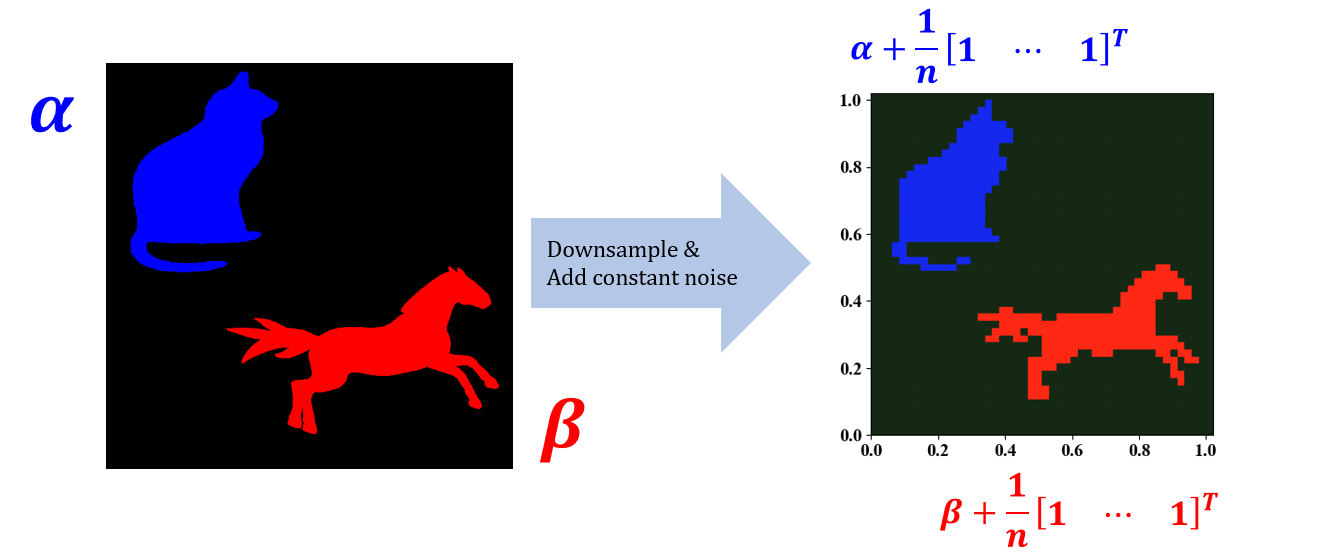
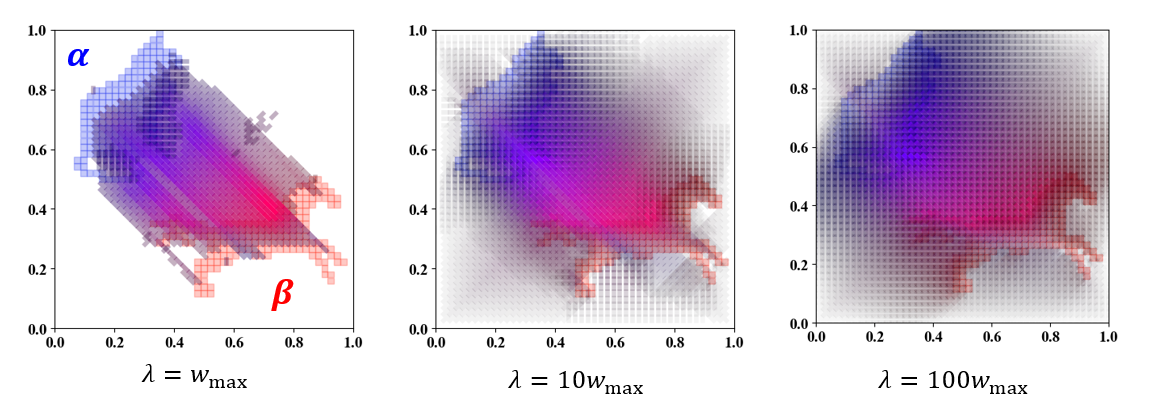
Figure 2. (Top row) images of a blue cat and red horse ($\alpha$ and $\beta$ resp.) are downsampled via nearest neighbors to $G$, which is embedded in the unit square. (Bottom row) the optimal flow of mass $J$ between the cat and the horse is visualized on $\delta$-active edges ($\delta=0.009$). The cat and horse are rendered below the optimal flow to improve the visualization. The flows for different values of $\lambda$ proportional to $w_{\mathrm{max}}:=\max_{e\in E^{\prime}}w(e)$ are shown. Note that as $\lambda$ increases, the flow becomes less localized near the input images. $\lambda<<w_{\mathrm{max}}$ leads to unstable results.

4.4. Transporting pseudo-conic densities

Here we analyze the the alterations in the optimal flow as we manipulate the signatures on specific edges within the graph. We begin with the graph $\mathcal{G}_{s}$ equipped with the $2$-dimensional trivial connection ($d=2$). Here we consider two-dimensional localized psuedo-conic densities that are represented as conic density in one channel and uniform density in the other (these can be viewed as a generalization of the pseudo-Diracs described in Section 4.2). In particular, we consider two pseudo-conics in the red and blue channels that are positioned near the diagonally opposite ends of the square with a radius of $0.1$ (Figure 3). As expected, the optimal flow continuously moves the mass from the red channel to the blue channel as reflected in the gradual transition of colors from red to magenta to blue on the active edges along the diagonal.

Following this, we focus on the horizontal edges along the green line (Figure 3). We alter the signature along these edges from identity to the reversal matrix $\begin{bmatrix}0&1\\ 1&0\end{bmatrix}$. In contrast to the trivial connection, the optimal flow now primarily transports mass within a single channel on either side of the dashed line. The transport unfolds as follows: the mass is first carried from the support of the red conic density along the red channel up to the dashed-line. At this juncture, the edges with the reversal matrix as the signature trigger a complete mass transition from the red to the blue channel. Subsequently, the flow guides the mass along the blue channel towards its intended destination.

Finally, we examine another modification of the trivial connection graph. This involves changing the signature on the edges located within a circular disk from the identity to the reversal matrix (Figure 3). The resulting optimal flow transfers the mass along the red channel up to the boundary of the disk. At the boundary, the mass undergoes an equal distribution across both channels, evident from the magenta coloring of the edges. This outcome aligns with the invariance of a constant vector to the reversal operator. Eventually, the entire mass is directed towards the blue channel as the flow moves beyond the boundary of the disk.

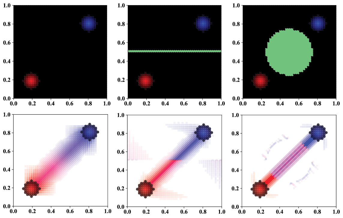
Figure 3. (Left column) the graph $\mathcal{G}_{s}$ is equipped with a trivial connection. (Middle column) the signature on the edges along the green horizontal line are set to the reversal matrix. (Right column) the signature on the edges in the green circular disk is set to the reversal matrix. (First row) The red and blue pseudo-conics represent the source and destination density, respectively. (Second row) the optimal flow of mass $J$ from source to destination densities is visualized on $\delta$-active edges ($\delta=2.5\times 10^{-4}$). The source and destination densities are also shown to improve visualization.

We repeat a similar set of experiments on the graph $\mathcal{G}_{t}$ on a torus. We examine the nature of the optimal flow between two localized conic densities, both in the context of the trivial connection graph and its alterations (Figure 4). We first obtain the optimal flow corresponding to the trivial connection where we observe a similar behavior as before: the mass transitioning from red to magenta and finally to blue along edges that trace shorter paths between the supports of the two densities. We further visualize the optimal flow on the intrinsic parameterization of the torus. This provides a contrast to the (expected) vertical-oriented optimal flow between conic densities on a square grid. Notably, the curvature inherent to this flow’s trajectory encapsulates the manifold’s intricate geometry. Subsequently, we introduce alterations to the trivial signature: first on the edges circumventing the tube via dashed loops, while the second pertains to edges within the tubular regions (Figure 4). In both cases, the signature on the edges are switched to the reversal matrix. We observe in both instances that the flow’s essential nature remains similar to that observed on a square grid.

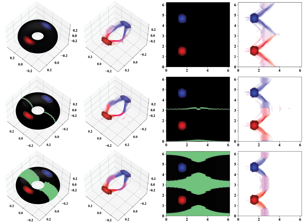
Figure 4. In each row, the third and fourth plots depict the first and second plots, respectively, adapted to the intrinsic parameterization of the torus. (Top row) the graph $\mathcal{G}_{t}$ is equipped with a trivial connection. (Middle row) the signature on the edges along the two green loops are switched from the identity to the reversal matrix. (Bottom row) the signature on the edges in the green tubular regions is set to the reversal matrix. (First column) The pseudo-conic source (red) and destination (blue) densities are visualized on the curved torus. (Second column) the optimal flow of mass $J$ between the two densities is visualized on $\delta$-active edges ($\delta=2.5\times 10^{-4}$). The source and destination densities are also shown to improve visualization.

4.5. Transporting conic densities

In the following experiments, instead of employing pseudo-conics, we will utilize conic densities in both channels, each centered at distinct locations (Figure 5 and Figure 6). Specifically, in the context of the square grid, the source density is represented by the four half-conics located near the boundary, while the destination density is characterized by the conics positioned along the central vertical line. In the case of the torus, the source density constitutes the two conics situated on the outer part of the surface, while the destination density is formed by those near the hole.

We once again explore three different configurations of the connection graph: (a) A trivial signature applied to all edges, (b) a reversal matrix assigned to the edges along the two vertical lines in the case of the square grid, and along the top and bottom circular loops in the case of the torus, and (c) a reversal matrix assigned to all edges within the green-colored regions.

In the context of the square grid with the trivial connection setup, the optimal flow essentially exhibits an independent transfer of mass along the two channels, rather than mixing the masses across the channels, as was the case with pseudo-conic densities. It appears that the curved geometry of the torus influences the optimal flow to some extent, leading to a redistribution of masses across the two channels. Moving on to the second connection graph, the incentive for shifting mass from one channel to the other is significant, resulting in a horizontal flow from the blue conics towards the red conics. Lastly, under the third configuration, mass tends to redistribute across the two channels as it flows over the bands of reversal matrices. However, unlike the scenario with pseudo-conic densities, this redistribution of mass is uneven across the two channels, resulting in a wave-like flow across the band instead of a uniform magenta flow.

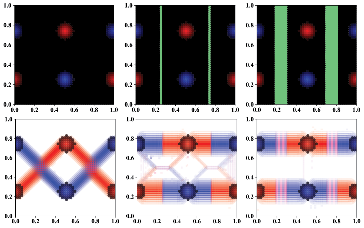
Figure 5. (Left column) the graph $\mathcal{G}_{s}$ is equipped with a trivial connection. (Middle column) the signature on the edges along the green vertical lines are set to the reversal matrix. (Right column) the signature on the edges in the green regions is set to the reversal matrix. (First row) The red and blue half-conics near the boundary of the square represent the source density. The two red and blue conics in the middle of the square represent the destination density. (Second row) the optimal flow of mass $J$ from source to destination densities is visualized on all the active edges. The source and destination densities are also shown to improve visualization.

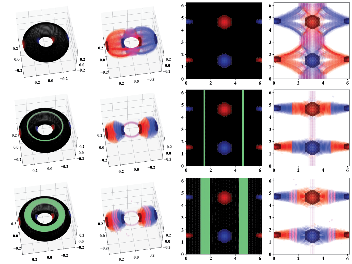
Figure 6. In each row, the third and fourth plots depict the first and second plots, respectively, adapted to the intrinsic parameterization of the torus. (Top row) the graph $\mathcal{G}_{t}$ is equipped with a trivial connection. (Middle row) the signature on the edges along the two circular loops are set to the reversal matrix. (Bottom row) the signature on the edges in the green regions is set to the reversal matrix. (First column) The red and blue conics on the outer surface of the torus represent the source density. Similarly, the conics on the inner surface represent the destination density. (Second column) the optimal flow of mass $J$ from source to destination densities is visualized on all the active edges. The source and destination densities are also shown to improve visualization.

References

- [1] A. S. Bandeira, A. Singer, and D. A. Spielman, A Cheeger inequality for the graph connection Laplacian, SIAM Journal on Matrix Analysis and Applications, 34 (2013), pp. 1611–1630.
- [2] F. Barbero, C. Bodnar, H. S. de Ocáriz Borde, M. Bronstein, P. Veličković, and P. Lio, Sheaf neural networks with connection Laplacians, in Topological, Algebraic and Geometric Learning Workshops 2022, PMLR, 2022, pp. 28–36.
- [3] T. Bhamre, T. Zhang, and A. Singer, Orthogonal matrix retrieval in cryo-electron microscopy, in 2015 IEEE 12th International Symposium on Biomedical Imaging (ISBI), IEEE, 2015, pp. 1048–1052.
- [4] J. Bigot, E. Cazelles, and N. Papadakis, Central limit theorems for entropy-regularized optimal transport on finite spaces and statistical applications, (2019).
- [5] N. Bonneel and J. Digne, A survey of optimal transport for computer graphics and computer vision, Computer Graphics Forum, 42 (2023), pp. 439–460.
- [6] S. P. Boyd and L. Vandenberghe, Convex optimization, Cambridge university press, 2004.
- [7] D. Cartwright and F. Harary, Structural balance: a generalization of Heider’s theory, Psychological review, 63 (1956), p. 277.
- [8] Y. Chen, T. T. Georgiou, and A. Tannenbaum, Vector-valued optimal mass transport, SIAM Journal on Applied Mathematics, 78 (2018), pp. 1682–1696.
- [9] F. Chung, W. Zhao, and M. Kempton, Ranking and sparsifying a connection graph, Internet Math., 10 (2014).
- [10] K. J. Ciosmak, Matrix Hölder’s inequality and divergence formulation of optimal transport of vector measures, SIAM J. Math. Anal., 53 (2021).
- [11] K. J. Ciosmak, Optimal transport of vector measures, Calculus of Variations and Partial Differential Equations, 60 (2021), p. 230.
- [12] A. Cloninger, K. Hamm, V. Khurana, and C. Moosmüller, Linearized Wasserstein dimensionality reduction with approximation guarantees, arXiv preprint arXiv:2302.07373, (2023).
- [13] A. Cloninger, G. Mishne, A. Oslandsbotn, S. J. Robertson, Z. Wan, and Y. Wang, Random walks, conductance, and resistance for the connection graph Laplacian, arXiv preprint arXiv:2308.09690, (2023).
- [14] A. Cloninger, B. Roy, C. Riley, and H. M. Krumholz, People mover’s distance: class level geometry using fast pairwise data adaptive transportation costs, Applied and Computational Harmonic Analysis, 47 (2019), pp. 248–257.
- [15] M. Essid and J. Solomon, Quadratically regularized optimal transport on graphs, SIAM J. Sci. Comput., 40 (2018).
- [16] J. D. Farmer, Extreme points of the unit ball of the space of Lipschitz functions, Proceedings of the American Mathematical Society, 121 (1994), pp. 807–813.
- [17] M. Feldman and R. McCann, Monge’s transport problem on a Riemannian manifold, Transactions of the American Mathematical Society, 354 (2002), pp. 1667–1697.
- [18] S. Ferradans, N. Papadakis, G. Peyré, and J.-F. Aujol, Regularized discrete optimal transport, SIAM Journal on Imaging Sciences, 7 (2014), pp. 1853–1882.
- [19] W. Gangbo and R. J. McCann, The geometry of optimal transportation, Acta Mathematica, 177 (1996), pp. 113–161.
- [20] V. Huroyan, G. Lerman, and H.-T. Wu, Solving jigsaw puzzles by the graph connection Laplacian, SIAM Journal on Imaging Sciences, 13 (2020), pp. 1717–1753.
- [21] L. V. Kantorovich, On the translocation of masses, in Dokl. Akad. Nauk. USSR (NS), vol. 37, 1942, pp. 199–201.
- [22] V. Khurana, H. Kannan, A. Cloninger, and C. Moosmüller, Supervised learning of sheared distributions using linearized optimal transport, Sampling Theory, Signal Processing, and Data Analysis, 21 (2023), p. 1.
- [23] D. Leite, D. Baptista, A. A. Ibrahim, E. Facca, and C. De Bacco, Community detection in networks by dynamical optimal transport formulation, Scientific Reports, 12 (2022), p. 16811.
- [24] E. H. Lieb and M. Loss, Fluxes, Laplacians, and Kasteleyn’s theorem, 2004.
- [25] H. Ling and K. Okada, An efficient earth mover’s distance algorithm for robust histogram comparison, IEEE transactions on pattern analysis and machine intelligence, 29 (2007), pp. 840–853.
- [26] A. Lonardi, M. Putti, and C. De Bacco, Multicommodity routing optimization for engineering networks, Scientific reports, 12 (2022), p. 7474.
- [27] G. Monge, Mémoire sur la théorie des déblais et des remblais, Mem. Math. Phys. Acad. Royale Sci., (1781), pp. 666–704.
- [28] C. Moosmüller and A. Cloninger, Linear optimal transport embedding: provable Wasserstein classification for certain rigid transformations and perturbations, Information and Inference: A Journal of the IMA, 12 (2023), pp. 363–389.
- [29] N. Papadakis, Optimal transport for image processing, PhD thesis, Université de Bordeaux, 2015.
- [30] G. Peyré and M. Cuturi, Computational optimal transport, Foundations and Trends in Machine Learning, 11 (2019), pp. 355–607.
- [31] E. K. Ryu, Y. Chen, W. Li, and S. Osher, Vector and matrix optimal mass transport: theory, algorithm, and applications, SIAM J. Sci. Comput., 40 (2018).
- [32] F. Santambrogio, Optimal transport for applied mathematicians, Birkäuser, NY, 55 (2015), p. 94.
- [33] A. Singer, Angular synchronization by eigenvectors and semidefinite programming, Applied and computational harmonic analysis, 30 (2011), pp. 20–36.
- [34] A. Singer and H.-T. Wu, Vector diffusion maps and the connection Laplacian, Communications on pure and applied mathematics, 65 (2012), pp. 1067–1144.
- [35] J. Solomon, Optimal transport on discrete domains, AMS Short Course on Discrete Differential Geometry, (2018).
- [36] J. Solomon, F. De Goes, G. Peyré, M. Cuturi, A. Butscher, A. Nguyen, T. Du, and L. Guibas, Convolutional Wasserstein distances: Efficient optimal transportation on geometric domains, ACM Transactions on Graphics (ToG), 34 (2015), pp. 1–11.
- [37] J. Solomon, R. Rustamov, L. Guibas, and A. Butscher, Earth mover’s distances on discrete surfaces, ACM Trans. Graph., 33 (2014).
- [38] Y. Tian and R. Lambiotte, Structural balance and random walks on complex networks with complex weights, arXiv preprint arXiv:2307.01813, (2023).