Abstract

Deep learning based methods for image reconstruction are state-of-the-art for a variety of imaging tasks. However, neural networks often perform worse if the training data differs significantly from the data they are applied to. For example, a network trained for accelerated magnetic resonance imaging (MRI) on one scanner performs worse on another scanner. In this work, we investigate the impact of the training data on the model’s performance and robustness for accelerated MRI. We find that models trained on the combination of various data distributions, such as those obtained from different MRI scanners and anatomies, exhibit robustness equal or superior to models trained on the best single distribution for a specific target distribution. Thus training on diverse data tends to improve robustness. Furthermore, training on diverse data does not compromise in-distribution performance, i.e., a model trained on diverse data yields in-distribution performance at least as good as models trained on the more narrow individual distributions. Our results suggest that training a model for imaging on a variety of distributions tends to yield a more effective and robust model than maintaining separate models for individual distributions.

1 Introduction

Deep learning models trained end-to-end for image reconstruction are fast and accurate and outperform traditional image reconstruction methods for a variety of imaging tasks ranging from denoising over super-resolution to accelerated MRI [Jin+17, Lia+21, Don+14, Muc+21].

Imaging accuracy is typically measured as in-distribution performance: A model trained on data from one source is applied to data from the same source. However, in practice a neural network for imaging is typically applied to slightly different data than it is trained on. For example, a neural network for accelerated magnetic resonance imaging trained on data from one hospital is applied in a different hospital.

Neural networks for imaging often perform significantly worse under such distribution shifts. For accelerated MRI, a network trained on knees performs worse on brains when compared to the same network trained on brains. Similar performance loss occurs for other natural distribution shifts [Kno+19, Joh+21, DCH21].

To date, much of research in deep learning for imaging has focused on developing better models and algorithms to improve in-distribution performance. Nevertheless, recent literature on computer vision models, in particular multi-modal models, suggest that a model’s robustness is largely impacted by the training data, and a key ingredient for robust models are large and diverse training sets [Fan+22, Ngu+22, Gad+23].

In this paper, we take a step towards a better understanding of the training data for learning robust deep networks for accelerated magnetic resonance imaging (MRI).

• First, we investigate whether deep networks for accelerated MRI compromise performance on individual distributions when trained on more than one distribution. We find for various pairs of distributions (different anatomies, image contrasts, and magnetic fields), that training a single model on two distributions yields the same performance as training two individual models.

• Second, we demonstrate for a variety of distribution shifts (anatomy shift, image contrast shift, and magnetic field shift) that the robustness of models, regardless of its architecture, is largely determined by the training set. A diverse set enhances robustness towards distribution shifts.

• Third, we consider a distribution shift from healthy to non-healthy subjects and find that models trained on a diverse set of healthy subjects can accurately reconstruct images with pathologies even if the model has never seen pathologies during training.

• Fourth, we empirically find for a variety of distribution shifts that distributional overfitting occurs: When training for long, in-distribution performance continues to improve slightly while out-of-distribution performance sharply drops. A related observation was made by [Wor+22] for fine-tuning of CLIP models. Therefore, early stopping can be helpful for training a robust model as it can yield a model with almost optimal in-distribution performance without losing robustness.

Taken together, those four findings suggest that training a single model on a diverse set of data distributions and incorporating early stopping yields a robust model. We test this hypothesis by training a model on a large and diverse pool of data significantly larger than the fastMRI dataset, the single largest dataset for accelerated MRI. We find that the resulting network is significantly more robust than a model trained on the fastMRI dataset, without compromising in-distribution performance.

Related Work.

A variety of influential papers have shown that machine learning methods for problems ranging from image classification to natural language processing perform worse under distribution shifts [Rec+19, Mil+20, Tao+20, Hen+21].

With regards to accelerated MRI, [Joh+21] evaluate the out-of-distribution robustness of the models submitted to the 2019 fastMRI challenge [Kno+20], and find that they are sensitive to distribution shifts. Furthermore, [DCH21] demonstrate that reconstruction methods for MRI, regardless of whether they are trained or only tuned on data, all exhibit similar performance loss under distribution shifts. Both works do not propose robustness enhancing strategies, such as training on a diverse dataset. Moreover, there are several works that characterise the severity of specific distribution-shifts and propose transfer learning as a mitigation strategy [Kno+19, Hua+22, Dar+20]. Those works fine-tune on data from the test distribution, whereas we study-out-of-distribution setup without access to the test distribution.

A potential solution to enhance robustness in accelerated MRI is test-time training to narrow the performance gap on out-of-distribution data [DLH22], albeit at high computational costs. In the context of ultrasound imaging, [KJ+23] demonstrate that diversifying simulated training data can improve robustness on real-world data. [Liu+21] propose a special network architecture to improve the performance of training on multiple anatomies simultaneously. [Ouy+23] proposes an approach that modifies natural images for training MRI reconstruction models.

Shifting to computer vision, OpenAI’s CLIP model [Rad+21] is robust under distribution shifts. [Fan+22] finds that the key contributor to CLIP’s robustness is the diversity of the training set. However, [Ngu+22] show that blindly combining data sources can weaken robustness compared to training on the best individual data source.

These studies underscore the pivotal role of dataset design, particularly data diversity, for a model’s performance and robustness. In light of concerns regarding the robustness of deep learning in medical imaging, we explore the impact of data diversity on models trained for accelerated MRI.

We also note that it is well known that increasing the training set size generally improves performance, and often this performance increase follows a power law, for language modelling [Kap+20], vision [Zha+22], and image reconstruction problems [KH23]. Contrary, in this paper we study out-of-distribution robustness improvements through diversity, as opposed to in-distribution improvements through data set size.

We finally note that in this paper we focus on out-of-distribution robustness, there are other robustness notions such as worst-case robustness [Ant+20, Duc+22, KSH23].

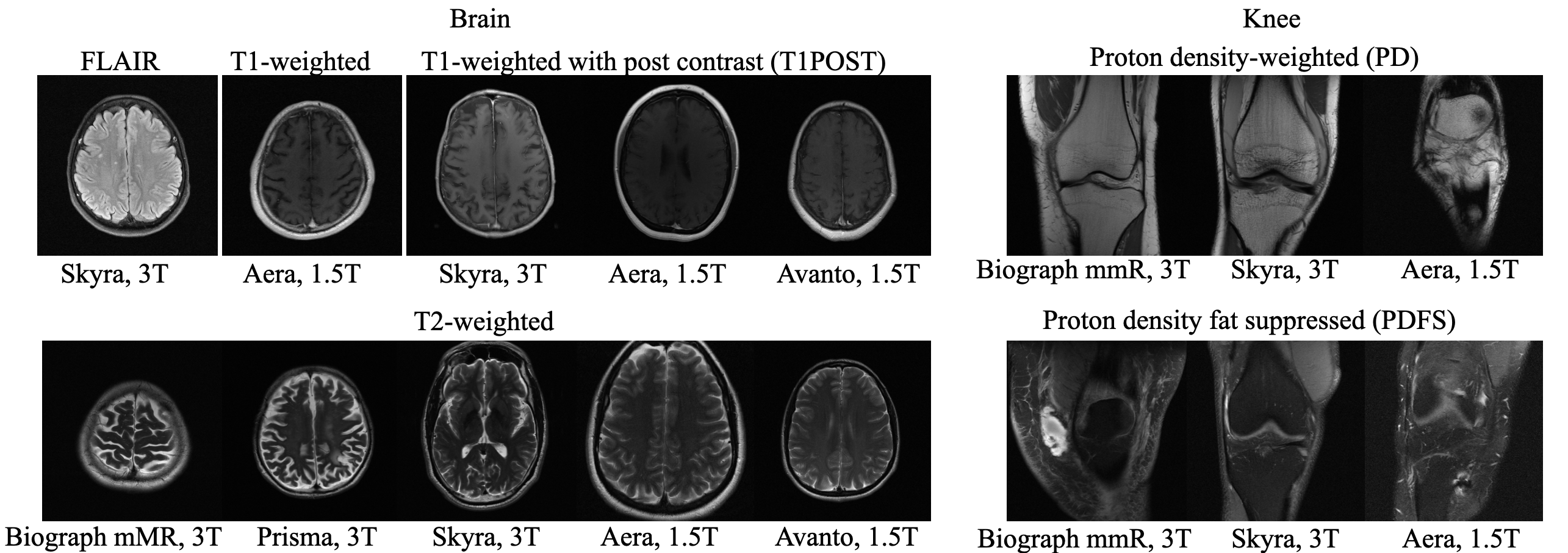
Figure 1: Example images for a selection of distributions from the fastMRI dataset [Zbo+19] we consider here. Axial view brain images are on the left, coronal view knee images are on the right. The caption above an image describes the image contrast, and the caption below is the name of the MRI scanner used.

2 Setup and background

Table 1: Fully-sampled k-space datasets used here. The percentages are the proportions of the data within a dataset. Scans containing multiple echoes or averages are separated as such and counted as separate volumes.

Dataset Anatomy View Image contrast Vendor Magnet Coils Vol./Subj. Slices fastMRI knee [Zbo+19] knee coronal PD (50%), PDFS (50%) Siemens 1.5T (45%), 3T (55%) 15 1.2k/1.2k 42k fastMRI brain [Zbo+19] brain axial T1 (11%), T1POST (21%), T2 (60%), FLAIR (8%) Siemens 1.5T (43%), 3T (67%) 4-20 6.4k/6.4k 100k fastMRI prostate [Tib+23] prostate axial T2 Siemens 3T 10-30 312/312 9.5k M4Raw [Lyu+23] brain axial T1 (37%), T2 (37%), FLAIR (26%) XGY 0.3T 4 1.4k/183 25k SKM-TEA, 3D [Des+21] knee sagittal qDESS GE 3T 8, 16 310/155 50k Stanford 3D [Epp13] knee axial PDFS GE 3T 8 19/19 6k Stanford 3D [Epp13] knee coronal PDFS GE 3T 8 19/19 6k Stanford 3D [Epp13] knee sagittal PDFS GE 3T 8 19/19 4.8k 7T database, 3D [Caa22] brain axial MP2RAGE-ME Philips 7T 32 385/77 112k 7T database, 3D [Caa22] brain coronal MP2RAGE-ME Philips 7T 32 385/77 112k 7T database, 3D [Caa22] brain sagittal MP2RAGE-ME Philips 7T 32 385/77 91k CC-359, 3D [Sou+18] brain axial GRE GE 3T 12 67/67 17k CC-359, 3D [Sou+18] brain coronal GRE GE 3T 12 67/67 14k CC-359, 3D [Sou+18] brain sagittal GRE GE 3T 12 67/67 11k Stanford 2D [Che18] various various various GE 3T 3-32 89/89 2k NYU data [Ham+18] knee various PD (40%), PDFS (20%), T2FS(40%) Siemens 3T 15 100/20 3.5k M4Raw GRE [Lyu+23] brain axial GRE XGY 0.3T 4 366/183 6.6k

We consider multi-coil accelerated MRI, where the goal is to reconstruct a complex-valued image $\mathbf{x}\in\mathbb{C}^{N}$ from the measurements of electromagnetic signals obtained through $C$ receiver coils according to

$$\mathbf{y}_{i}=\mathbf{M}\mathbf{F}\mathbf{S}_{i}\mathbf{x}+\mathbf{z}_{i}\in\mathbb{C}^{m},\quad i=1,\ldots,C.$$ (1)

Here, $\mathbf{S}_{i}$ is the sensitivity map of the $i$-th coil, $\mathbf{F}$ is the 2D discrete Fourier transform, $\mathbf{M}$ is an undersampling mask, and $\mathbf{z}_{i}$ models additive white Gaussian noise. The measurements $\mathbf{y}_{i}$ are often called k-space measurements.

In this work, we consider 4-fold accelerated (i.e., $m=N/4$) multi-coil 2D MRI reconstruction with 1D Cartesian undersampling. The central k-space region is fully sampled including 8% of all k-space lines, and the remaining lines are sampled equidistantly with a random offset from the start. We choose 4-fold acceleration as going beyond 4-fold acceleration, radiologists tend to reject the reconstructions by neural networks and other methods as not sufficiently good [Muc+21, Rad+22]. Equidistant sampling is chosen due to the ease of implementation on existing machines [Zbo+19].

Class of reconstruction methods.

We focus on deep learning models trained end-to-end for accelerated MRI, as this class of methods gives state-of-the-art performance in accuracy and speed [Ham+18, AMJ19, Sri+20, FTS22]. There are different approaches to image reconstruction with neural networks including un-trained neural networks [UVL20, HH19, DH21] and methods based on generative neural networks [Bor+17, Jal+21, ZKP23].

A neural network $f_{\bm{\theta}}$ with parameters ${\bm{\theta}}$ mapping a measurement $\mathbf{y}=\{\mathbf{y}_{1},\ldots,\mathbf{y}_{C}\}$ to an image is most commonly trained to reconstruct an image from the measurements $\mathbf{y}$ by minimizing the supervised loss $\mathcal{L}({\bm{\theta}})=\sum_{i=1}^{n}\text{loss}(f_{\bm{\theta}}(\mathbf{y}_{i}),\mathbf{x}_{i})$ over a training set consisting of target image and corresponding measurements $\{(\mathbf{x}_{1},\mathbf{y}_{1}),\ldots,(\mathbf{x}_{n},\mathbf{y}_{n})\}$. This dataset is typically constructed from fully-sampled k-space data (i.e., data where the undersampling mask $M$ is identity). From the fully-sampled k-space data, a target image $\mathbf{x}$ is estimated, and retrospectively undersampled measurements $\mathbf{y}$ are generated by applying the undersampling mask to the fully-sampled data.

Several choices of network architectures work well. A standard baseline is a U-net [RFB15] trained to reconstruct the image from a coarse least-squares reconstruction of the measurements [Zbo+19]. A vision transformer for image reconstruction applied in the same fashion as the U-net also works well [LH22]. The best-performing models are unrolled neural networks such as the variational network [Ham+18] and a deep cascade of convolutional neural networks [Sch+18]. The unrolled networks often use either the U-net as backbone, like the end-to-end VarNet [Sri+20], or a transformer based architecture [FTS22].

We expect our results in this paper to be model agnostic, and show that this is indeed the case for the U-net, ViT, and End-to-end VarNet.

Datasets.

We consider the fully-sampled MRI dataset with varying attributes listed in Table 1. The datasets include the largest publicly available fully-sampled MRI datasets.

Many of our experiments are based on splits of the fastMRI dataset [Zbo+19], the most commonly used dataset for MRI reconstruction research. Figure 1 depicts samples from the fastMRI dataset and shows that MRI data varies significantly in appearance across different anatomies and image contrasts (FLAIR, T1, PD, etc). The image distribution also varies across vendors and magnetic field strengths of scanners, as the strength of the magnet impacts the signal-to-noise ratio (SNR), with stronger magnets leading to higher SNRs.

The fastMRI dataset stands out for its diversity and size, making it particularly well-suited for exploring how different data distributions can affect the performance of deep learning models for accelerated MRI. In our experiments in Section 3, 4, 5, and 6 we split the fastMRI dataset according to different attributes of the data. In Section 7, we showcase the generalizability of our findings by training models on all the datasets listed in Table 1, excluding the last four rows, which are reserved for robustness evaluation.

3 Training a single model or separate models on different distributions

Figure 2: The orange and blue bars are the VarNet models trained exclusively on data from $P$ ( $\mathcal{D}_{P}$) and $Q$ ( $\mathcal{D}_{Q}$), respectively, and the teal bars are the models trained on both sets $\mathcal{D}_{P}\cup\mathcal{D}_{Q}$. As a reference point, the black bars are the performance of models trained on random samples of $\mathcal{D}_{P}\cup\mathcal{D}_{Q}$ of half the size. Below each bar is the total number of training images. We are in the high-data regime where increasing the dataset further gives only minor improvements. For all distributions, the joint model trained on $P$ and $Q$ performs as well on $P$ and $Q$ as the models trained individually for each of those distributions.

Figure 3: Training a single model on a slightly skewed dataset does not harm performance on the individual data distributions. The number below each bar is the number of training examples used. We report the mean $\pm$ two standard deviations from five runs, each with a different random seed for sampling training data from $P$ and model initialization. We note for training sets exceeding 3k images, there is next to no variation (see Figure 11), therefore we only have error bars for this experiment which includes training runs on small datasets.

We start with studying whether training a model on data from a diverse set of distributions compromises the performance on the individual distributions. In its simplest instance, the question is whether a model for image reconstruction trained on data from both distributions $P$ and $Q$ performs as well on distributions $P$ and $Q$ as a model trained on $P$ and applied on $P$ and a model trained on $Q$ and applied on $Q$.

In general, this depends on the distributions $P$ and $Q$, and on the estimator. For example, consider a simple toy denoising problem, where the data from distribution $P$ is generated as $\mathbf{y}=\mathbf{x}+\mathbf{e}$, with $\mathbf{x}$ is drawn i.i.d. from the unit sphere of a subspace, and $\mathbf{e}$ is drawn from a zero-mean Gaussian with co-variance matrix $\sigma_{P}\mathbf{I}$. Data for distribution $Q$ is generated equally, but the noise is drawn from a zero-mean distribution with different noise variance, i.e., $\mathbf{e}\sim\mathcal{N}(0,\sigma_{Q}^{2}\mathbf{I})$ with $\sigma_{P}^{2}\neq\sigma_{Q}^{2}$. Then the optimal linear estimator learned from data drawn from both distribution $P$ and $Q$ is sub-optimal for both distributions $P$ and $Q$. However, there exists a non-linear estimator that is as good as the optimal linear estimator on distribution $P$ and distribution $Q$.

In addition, conventional approaches to MRI such as $\ell_{1}$-regularized least-squares need to be tuned individually on different distributions to achieve best performance, as discussed in Appendix A.

Thus it is unclear whether it is preferable to train a neural network for MRI on diverse data from many distributions or to train several networks and use them for each individual distribution. For example, is it better to train a network specific for knees and another one for brains or to train a single network on knees and brains together? Here, we find that training a network on several distributions simultaneously does not compromise performance on the individual distribution relative to training one model for each distribution.

Experiments for training a joint or separate models.

We consider two distributions $P$ and $Q$, and train VarNets [Sri+20], U-nets [RFB15], and ViTs [LH22] on data $\mathcal{D}_{P}$ from distributions $P$ and on data $D_{Q}$ from distribution $Q$ separately. We also train a VarNet, U-net, and ViT on data from $P$ and $Q$, i.e., $\mathcal{D}_{P}\cup\mathcal{D}_{Q}$. We then evaluate on separate test sets from distribution $P$ and $Q$. We consider the VarNet because it is a state-of-the-art model for accelerated MRI, and consider the U-net and ViT as popular baseline models to demonstrate that our qualitative results are independent of the architecture. We consider the following choices of the datasets $\mathcal{D}_{P}$ and $\mathcal{D}_{Q}$, which are subsets of the fastMRI dataset specified in Figure 1:

• Anatomies. $P$ are knees scans collected with 6 different combinations of image contrasts and scanners and $Q$ are the brain scans collected with 10 different combinations of image contrasts and scanners.

• Contrasts. We select $P$ as PD-weighted knee images from 3 different scanners and $Q$ are PDFS-weighted knee images from the same 3 scanners.

• Magnetic field. Here, we pick $P$ to contain all 3.0T scanners and $Q$ to contain all 1.5T scanners regardless of anatomy or image contrast.

The results in Figure 3 for VarNet show that the models trained on both $P$ and $Q$ achieve essentially the same performance on both $P$ and $Q$ as the individual models. The model trained on both $P+Q$ uses more examples than the model trained on $P$ and $Q$ individually. To rule out the possibility that the joint model is only as good as the individual models since it is trained on more examples, we also trained a model on $P+Q$ with half the number of examples (obtained by randomly subsampling). Again, the model performs essentially equally well as the other models. We refer to Appendix B.1 and B.2 for details regarding the experiment setup.

The results for U-net and ViT are qualitatively the same as the results in Figure 3 for VarNet (see Appendix B.3), and indicate that our findings are independent of the architecture used.

Thus, separating datasets into data from individual distributions and training individual models does not yield benefits, unlike for $\ell_{1}$-regularized least squares or the toy-subspace example.

Experiments for training a joint or separate models on skewed data.

Next, we consider skewed data, i.e., the training set $\mathcal{D}_{P}$ is by a factor of about $10$ smaller than the training set $\mathcal{D}_{Q}$. The choices for distributions $P$ and $Q$ are as in the previous experiment. The results in Figure 3 show that even for data skewed by a factor 10, the performance on distributions $P$ and $Q$ of models (here U-net) trained on both distributions is comparable to the models trained on the individual distributions.

4 Data diversity enhances robustness towards distribution shifts

We now study how training on diverse data affects the out-of-distribution performance of a model. We find that training a model on diverse data improves a models out-of-distribution performance.

Figure 4: For a distribution-shift from distributions $P=\{P_{1},\ldots,P_{m}\}$ to distribution $Q$, we compare robustness of models trained on $P$ (orange) to baselines trained on the best single distribution $P_{\text{best}}$ (violet). As additional reference, we also report models trained on both $P$ and $Q$ to imitate ideally robust models (teal). For the three distribution shifts shown, training on the more diverse dataset $P$ is beneficial compared to training on $P_{\text{best}}$ alone.

Measuring robustness.

Our goal is to measure the expected robustness gain by training models on diverse data, and we would like this measure to be independent of the model itself that we train on. We therefore measure robustness with the notion of effective robustness by [Tao+20]. We evaluate models on a standard in-distribution test set (i.e., data from the same source that generated the training data) and on an out-of-distribution test set. We then plot the out-of-distribution performance of a variety of models as a function of the in-distribution performance, see Figure 4.

It can be seen that the in- and out-of-distribution performance of models trained on data from one distribution, (e.g., in-distribution data violet) is well described by a linear fit. Thus, a dataset yields more effective robustness if models trained on it lie above the violet line, since such models have higher out-of-distribution performance for fixed in-distribution performance.

Experiment.

We are given data from two distributions $P$ and $Q$, where distribution $P$ can be split up into $m$ sub-distributions $P_{1},\ldots,P_{m}$. We consider the following choices for the two distributions, all based on the knee and brain fastMRI datasets illustrated in Figure 1:

• Anatomy shift: $P_{1},\ldots,P_{6}$ is knee data collected with 6 different combinations of image contrasts and scanners, and $Q$ are the different brain datasets collected with 8 different combinations of image contrasts and scanners. To mitigate changes in the forward map (1) on this distribution shift, we excluded the brain data from the scanner Avanto as this data was collected with significantly fewer coils compared to the data from the knee distributions.

• Contrast shift: $P_{1},\ldots,P_{5}$ are FLAIR, T1POST, or T1-weighted brain images and $Q$ are T2-weighted brain data.

• Magnetic field shift: $P_{1},\ldots,P_{7}$ are brain and knee data collected with 1.5T scanners (Aera, Avanto) regardless of image contrast and $Q$ are brain and knee data collected with 3T scanners (Skyra, Prisma, Biograph mMR) regardless of image contrast.

For each of the distributions $P_{1},\ldots,P_{m}$ we construct a training set with 2048 images and a test set with 128 images. We then train U-nets on each of the distributions $P_{1},\ldots,P_{m}$ separately and select from these distributions the distribution $P_{\text{best}}$ that maximizes the performance of the U-net on a test set from the distribution $Q$.

Now, we train a variety of different model architectures including the U-net, End-to-End VarNet [Sri+20], and vision transformer (ViT) for image reconstruction [LH22] on data from the distribution $P_{\text{best}}$, data from the distribution $P$ (which contains $P_{\text{best}}$), and data from the distribution $P$ and $Q$. We also sample different models by early stopping and by decreasing the training set size by four. We plot the performance of the models evaluated on the distribution $Q$ as a function of their performance evaluated on the distribution $P_{\text{best}}$. The configurations of our models are the same as in Section 3.

From the results in Figure 4 we see that the models trained on $P$ are outperformed by the model trained on $P$ and $Q$ when evaluated on $Q$, as expected, since a model trained on $P$ and $Q$ is an ideal robust baseline (as it contains data from $Q$). The difference of the trained on $P$ and $Q$-line and the trained on $P_{\text{best}}$-line is a measure of the severity of the distribution shift, as it indicates the loss in performance when a model trained on $P_{\text{best}}$ is evaluated on $Q$. Comparing the difference between the line for the models trained on $P$ and the line for models trained on $P_{\text{best}}$ shows that out-of-distribution performance is improved by training on a diverse dataset, even when compared to the distribution $P_{\text{best}}$ which is the most beneficial distribution for performance on $Q$.

5 Reconstruction of pathologies using data from healthy subjects

Figure 5: Models trained on images without pathologies can reconstruct pathologies as effectively as models trained on images with pathologies. SSIM is calculated only for the pathology region ($\bm{A}$) for small pathologies (left) and for large pathologies (right).

Figure 6: Reconstructions given by the VarNet of images containing a small-sized (top) or a large-sized (bottom) pathology, when trained on images without pathologies ($P$), and on images without and with pathologies ($P+Q$).

In this section, we investigate the distribution shift from healthy to non-healthy subjects by measuring how well models reconstruct images containing a pathology if no pathologies are contained in the training set. We find that models trained on fastMRI data without pathologies reconstruct fastMRI data with pathologies equally well as the same models trained on fastMRI data with pathologies.

Experiment.

We rely on the fastMRI+ annotations [Zha+22a] to partition the fastMRI brain dataset into disjoints sets of images with and without pathologies. The fastMRI+ annotations [Zha+22a] are annotations of the fastMRI knee and brain datasets for different types of pathologies. We extract a set of volumes without pathologies by selecting all scans with the fastMRI+ label “Normal for age”, and we select images with pathologies by taking all images with slice-level annotations of a pathology. The training set contains 4.5k images without pathologies ($P$) and 2.5k images with pathologies ($Q$). We train U-nets, ViTs, and VarNets on $P$ and on $P+Q$, and sample different models by varying the training set size by factors of 2, 4 and 8, and by early stopping. While the training set from distribution $P$ does not contain images with pathologies, $P$ is a diverse distribution containing data from different scanners and with different image contrasts.

Figure 5 shows the performance of each model evaluated on $Q$ as a function of its performance evaluated on $P$. Reconstructions are evaluated only on the region containing the pathology, where we further distinguish between small pathologies that take up less than $1\%$ of the total image size and large pathologies that take up more than $1\%$ of the total image size.

We see that the models trained on $P$ show essentially the same performance (SSIM) as models trained on $P+Q$ regardless of pathology size. The results indicate that models trained on images without pathologies can reconstruct pathologies as accurately as models trained on images with pathologies. This is further illustrated in Figure 6 (and Figure 16), where we show reconstructions given by the VarNet of images with a pathology: the model recovers the pathology well even though no pathologies are in the training set. Figure 14 in the appendix provides a more nuanced evaluation of the SSIM values for VarNet.

Figure 7: For a distribution shift from distribution $P$ to distribution $Q$, the in- and out-of-distribution performance is plotted as a function of training epochs (1, 5, 15, 30, 45, 60). At the beginning of training, out-of-distribution performance increases together with in-distribution performance. Then, out-of-distribution performance starts to drop while in-distribution performance continues to marginally increase.

6 Distributional overfitting

We observed that when training for long, while in-distribution performance continues to improve slightly, out-of-distribution performance can deteriorate. We refer to this as distributional overfitting. Unlike conventional overfitting, where a model’s in-distribution performance declines after prolonged training, distributional overfitting involves a decline in out-of-distribution performance while in-distribution performance continues to improve (slightly).

A similar observation has been made in the context of weight-space ensemble fine-tuning of CLIP [Wor+22].

Figure 7 illustrates distributional overfitting on three distribution shifts. Each plot depicts the in and out-of-distribution ($P$ and $Q$) performance of an U-net as a function of trained epochs (1, 5, 15, 30, 45, 60). For example, in the left plot $P$ is fastMRI T2-weighted brain data (fm brain, T2) and $Q$ is fastMRI knee data (fm knee). We observe as training progresses, initially, the model in-distribution and out-of-distribution performance both improves. However, after epoch 15, out-of-distribution performance deteriorates, despite marginal improvements in in-distribution performance. This pattern consistently occurs across distribution shifts from the fastMRI brain/knee dataset to the M4Raw dataset and the fastMRI prostate dataset.

This finding indicates that early stopping, even before conventional overfitting sets in, can help to improve model robustness with minimal impact on in-distribution performance.

7 Robust models for accelerated MRI

Figure 8: Training on a diverse collection of datasets improves robustness under distribution shifts. A model trained on the diverse set of datasets $\mathcal{D}_{P}$ can significantly outperform models trained on fastMRI data when evaluated on out-of-distribution data $\mathcal{D}_{Q}$, while maintaining the same performance on fastMRI data.

Figure 9: Random selection of reconstructions for two out-of-distribution datasets given by the VarNet trained on fastMRI knee (fm-knee), fastMRI brain (fm-brain), and collection of datasets $\mathcal{D}_{P}$. The model trained on $\mathcal{D}_{P}$ provides better details and fewer artifacts.

The results from the previous sections based on the fastMRI dataset suggest that training a single model on a diverse dataset consisting of data from several data distributions is beneficial to out-of-distribution performance without sacrificing in-distribution performance on individual distributions.

We now move beyond the fastMRI dataset and demonstrate that this continues to hold on a large collection of datasets. We train a single large model for 4-fold accelerated 2D MRI reconstruction on the first 13 of the datasets in Table 1, which include the fastMRI brain and knee datasets, and use the remaining four datasets for out-of-distribution evaluation. The resulting model, when compared to models trained only on the fastMRI dataset, shows significant robustness improvements while maintaining its performance on the fastMRI dataset.

Experiment.

We train an U-net, ViT, and a VarNet on the first 13 datasets in Table 1. We denote this collection of datasets by $\mathcal{D}_{P}$. For the fastMRI knee and brain datasets, we exclude the fastMRI knee validation set and the fastMRI brain test set from the training set, as we use those for testing. For the other datasets, we convert the data to follow the convention of the fastMRI dataset and omit slices that contain pure noise. The total number of training slices after the data preparation is 413k. For each model family, we also train a model on fastMRI knee, and one on fastMRI brain as baselines. To mitigate the risk of distributional overfitting, we early stop training when the improvement on the fastMRI knee dataset becomes marginal. Further experimental details are in Appendix F.

The fastMRI knee validation and fastMRI brain test set are used to measure in-distribution performance. We measure out-of-distribution performance on the last four datasets in Table 1, i.e., CC-359 sagittal view, Stanford 2D, M4Raw GRE, and NYU data. These datasets constitute a distribution shift relative to the training data with respect to vendors, anatomic views, anatomies, time-frame of data collection, anatomical views, MRI sequences, contrasts and combinations thereof and therefore enable a broad robustness evaluation. As a further reference point we also train models on the out-of-distribution datasets to quantify the robustness gap.

The results in Figure 8 show that for all architectures considered, the model trained on the collection of datasets, $\mathcal{D}_{P}$ significantly outperforms the models trained on fastMRI data when evaluated on out-of-distribution data, without compromising performance on fastMRI data. For example, on the CC-359 sagittal view dataset, the VarNet trained on $\mathcal{D}_{P}$ almost closes closes the distribution shift performance gap (i.e., the gap to the model trained on the out-of-distribution data). This robustness gain is illustrated in Figure 9 with examples images: the out-of-distribution images reconstructed by the model trained on the diverse dataset $\mathcal{D}_{P}$ have higher quality and fewer artifacts.

The results in this section reinforce our earlier findings, affirming that large and diverse MRI training sets can significantly enhance robustness without compromising in-distribution performance.

8 Conclusion and limitations

While our research shows that diverse training sets significantly enhances out-of-distribution robustness for deep learning models for accelerated MRI, training a model on a diverse dataset often doesn’t close the distribution shift performance gap, i.e., the gap between the model and the same idealized model trained on the out-of-distribution data (see Figure 4 and 8). Nevertheless, as datasets grow in size and diversity, training networks on larger and even more diverse data might progressively narrow the distribution shift performance gap. However, in practice it might be difficult or expensive to collect diverse and large datasets.

Besides demonstrating the effect of diverse training data, our work shows that care must be taken when training models for long as this can yield to a less robust model due to distributional overfitting. This finding also emphasizes the importance of evaluating on out-of-distribution data.

Reproducibility statement

Our code is available at https://github.com/MLI-lab/mri_data_diversity. All datasets used in this work are referenced and publicly available. For the implementation of our experiments, we heavily rely on the code provided by the fastMRI GitHub repository https://github.com/facebookresearch/fastMRI/tree/main.

Acknowledgements

This work was supported by the Bavarian Ministry of Economic Affairs, Regional Development and Energy as part of the project “6G Future Lab Bavaria”. This work also received support by the Institute of Advanced Studies at the Technical University of Munich and the Deutsche Forschungsgemeinschaft (DFG, German Research Foundation) - 456465471, 464123524.

Appendix A $\ell_{1}$-regularized least squares requires different hyperparameters on different distributions

The traditional approach for accelerated MRI is $\ell_{1}$-regularized least-squares [LDP07]. While $\ell_{1}$-regularized least-squares is not considered data-driven, the regularization hyperparameter it typically chosen in a data-driven manner. For different distributions like different anatomies or contrasts, the regularization parameter takes on different values and thus the method needs to be tuned separately for different distributions. This can be seen for example from Table 4 of [Zbo+19].

To demonstrate this, we performed wavelet-based $\ell_{1}$-regularized least-squares on the single-coil knee version of the fastMRI dataset [Zbo+19] using 100 images from distribution $P$: PD Knee Skyra, 3.0T and 100 from distribution $Q$: PDFS Knee Aera, 1.5T. Using a regularization weight $\lambda=0.01$ on distribution $P$ gives a SSIM of $0.792$, while $\lambda=0.001$ yields subpar SSIM of $0.788$. Contrary, on distribution $Q$, $\lambda=0.01$ only yields $0.602$, while $\lambda=0.001$ yields SSIM $0.609$. Thus, using the same model (i.e., the same regularization parameter for both distributions) is suboptimal for $\ell_{1}$-regularized. least squares. We used the BART https://mrirecon.github.io/bart/ for running $\ell_{1}$-regularized least squares.

Appendix B Experimental details and additional results for Section 3

B.1 Data preparation

For each of the distributions in Figure 1, we randomly sample volumes from the fastMRI training set for training so that the total number of slices is around 2048, and we randomly sample from the validation set for testing so that the number of test slices is around 128. Training sets of combination of distributions are then constructed by aggregating the training data from the individual distributions. For example, if we consider distribution $P$ to contain all six knee distributions from Figure 1, then the corresponding training set has $6\cdot 2048$ training images. Likewise, if $Q$ is for example all T2-weighted brain images the corresponding training set has $5\cdot 2048$ training images.

B.2 Models, training, and evaluation

Our configuration of the End-to-end VarNet [Sri+20] contains 8 cascades, each containing an U-net with 4 pooling layers and 12 channels in the first pooling layer. The sensitivity-map U-net of the VarNet has 4 pooling layers and 9 channels in the first pooling layer. The code for the model is taken from fastMRI’s GitHub repository.

The U-nets used in the experiments have 4 pooling layers and 32 channels in the first pooling layer. The implementation of the model is taken from the fastMRI GitHub repository. Our configuration of the vision transformer (ViT) for image reconstruction is the ViT-S configuration from [LH22], and the code is taken from the paper’s GitHub repository. For the model input of the U-net and ViT, we first fill missing k-space values with zeros, then apply 2D-IFFT, followed by a root-sum-of-squares (RSS) reconstructions to combine all the coil images into one single image, and lastly normalize it to zero-mean and unit-variance. The mean and variance are added and multiplied back to the model output, respectively. This is a standard prepossessing step, see for example fastMRI’s GitHub repository. The models are trained end-to-end with the objective to maximize SSIM between output and ground-truth.

For any model and any choice of distributions $P$ or $Q$, the models are trained for a total of 60 epochs and we use the Adam optimizer with $\beta_{1}=0.9$ and $\beta_{2}=0.999$. The mini-batch size is set to 1. We use linear learning-rate warm-up until a learning-rate of 1e-3 is reached and linearly decay the learning rate to 4e-5. The warm up period amounts to 1% of the total number of gradient steps. Gradients are clipped at a global $\ell_{2}$-norm of 1. During training, we randomly sample a different undersampling mask for each mini-batch independently.

During evaluation, for each volume we generated an undersampling mask randomly, and this mask is then used for all slices within the volume.

The learning-rate for each model is tuned based on a grid search on the values {1.3e-3, 1e-3, 7e-4, 4e-4} and training on a random subset (2k slices) of the fastMRI dataset. We found negligible differences between learning rates {1.3e-3, 1e-3, 7e-4} and therefore keep the learning rate to 1e-3 for simplicity. We also performed the same grid search on fastMRI subsets for PD-weighted knee and PDFS knee scans and made the same observations.

ViT

  U-net

  U-net-small

Figure 10: The orange and blue bars are the ViT (Top) and U-net (Middle) trained exclusively on data from $P$ ( $\mathcal{D}_{P}$) and $Q$ ( $\mathcal{D}_{Q}$), respectively, and the teal bars are the models trained on both sets $\mathcal{D}_{P}\cup\mathcal{D}_{Q}$. As a reference point, the black bars are the performance of models trained on random samples of $\mathcal{D}_{P}\cup\mathcal{D}_{Q}$ of half the size. The number below each bar is the total number of training images. It can be seen that we are in the high-data regime where increasing the dataset further gives minor improvements. For all distributions, the joint model trained on $P$ and $Q$ performs as well on $P$ and $Q$ as the models trained individually for each of those distributions. Similar results can observed when decreasing the size of the U-net by a factor of 10 (U-net-small, 757k parameters, Bottom).

B.3 Results for U-net and ViT

In the main body we presented results for the VarNet, here we present results for the U-net and ViT. In Figure 10, we see that, like for the VarNet discussed in the main body, for the U-net and ViT training on two distributions gives the same performance as separate models trained on the individual distributions. Moreover, Figure 11 shows the same experiment for the U-net on smaller datasets, where the same observation can be made.

Figure 11: Also for smaller sized datasets, a single model performs at least as good as separate models. We report the mean $\pm$ two standard deviations from five runs with the U-net, each with a different random seed for sampling training data and model initialization. Note that when training on datasets with more than 3k images, there is next to no variation.

Table 2: A model trained on data with various acceleration factors (2, 4, 8, 16-fold) performs comparable as models trained individually for each acceleration factor. Additionally, the model trained on various acceleration factors can enhance performance for unseen acceleration factors (3-fold). Models were trained and evaluated on the fastMRI PDFS knee subset.

2-fold 4-fold 8-fold 16-fold 3-fold 2-fold 0.945 — — — 0.906 4-fold — 0.903 — — 0.899 8-fold — — 0.867 — 0.834 16-fold — — — 0.828 0.758 All of above 0.944 0.902 0.866 0.829 0.912 3-fold — — — — 0.921

Appendix C Distribution shifts induced by forward model changes

In the main body, we considered distribution shifts primarily related to the images, such as different contrast and anatomies. In this section, we consider two distribution shifts that are induced by changes of the forward model, i.e., the relation of measurements and object to be imaged. We consider shifts in the acceleration factor and a distribution shift related to the number of coils.

C.1 Results for training with multiple acceleration factors

In the main body, we presented reults for a single accelerated factor of 4.

We now train a (U-net) model simultaneously on data with 2-fold, 4-fold, 8-fold, and 16-fold acceleration factors, and analyze how the performance compares to U-net models trained for each acceleration separately. We train only on the fastMRI PDFS knee scans (see Figure 1). We report the performance in SSIM for each model and for each acceleration factor in Table 2. We also evaluate each model on 3-fold acceleration to see how combining different accelerations affects robustness towards a distribution-shifts related to the acceleration factor.

In Table 2, we see that the model trained on all four acceleration factors simultaneously (5th row) yields similar performance as the models trained individually on each acceleration factor (the differences in performance are within 0.001 SSIM, which is negligible).

For the out-of-distribution setup (i.e., evaluation on 3-fold acceleration), we observe that the model trained on all acceleration performs by 0.006 SSIM better relative to the best separately trained model (2-fold acceleration).

Taken together, these two observations suggest that training on combinations of different acceleration factors can increase the effective robustness of a model towards distribution-shifts related to changes to the acceleration factor slightly.

C.2 Distribution-shifts related to number of receive coils

We now consider a shift in the number of receive coils. For distribution $P$, we select all knees scans collected with the 6 different combinations of image contrasts and scanners (see Figure 1). All knee scans are collected with 15 coils. For distribution $Q$, we select the brain scans from the scanner Avanto since measurements from this scanner are collected with 4 coils.

For this distribution shift we noticed that models, in particular VarNet which estimates sensitivity maps, struggles to accurately predict the mean value of the images resulting in a noticeable drops in SSIM. However, this degradation was hardly noticeable when looking at the reconstructions. Given that radiologists routinely adjust the brightness and contrast of MRI images during inspection through a process known as windowing [Ish+84], we normalize the model output and target to have the same mean and variance during evaluation. The results are depicted in Figure 12, where we see that training on a diverse set $P$ increases effective robustness on this distribution shift.

Figure 12: Training on a diverse dataset ($P$) increases effective robustness under distribution-shifts related to the number of coils.

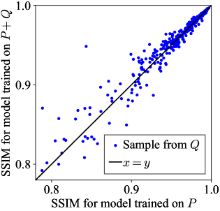
Figure 13: Reconstruction performance for each small pathology reconstructed with a VarNet trained only on data without pathologies (i.e., $P$) relative to the performance of a VarNet trained on data with and without pathologies ($P$ and $Q$). SSIM is measured only within the region containing the pathology. The majority of pathologies are reconstructed similarly well by both models, however in the regime where SSIM is low some images are reconstructed better by the P-model and others are reconstructed better by the $P+Q$-model.

Figure 14: Models trained only on images without pathologies and models trained on images with pathologies have similar global SSIM. Different models are sampled by varying the training set size by factors of 2, 4 and 8, and by early stopping.

Appendix D Additional results for Section 5

Figure 14 presents the reconstruction performance evaluated for individual images in the test set, focusing on small pathologies. The evaluation specifically targeted the pathology regions. Results are provided for VarNet trained solely on images without pathologies ($P$) and VarNet trained on images with and without pathologies ($P+Q$). Both models exhibit similar mean SSIM values for test images without pathology (approximately 0.957 SSIM) and also similar SSIM values for test images with small pathologies (approximately 0.948 SSIM).

Both models perform well for the majority of samples, indicated by high SSIM scores. In the low-SSIM regime where the SSIM is low for both models, some samples are better reconstructed by the model trained on $P+Q$ and some are better reconstructed by the model trained solely on $P$.

In Figure 14, we show reconstruction performance when SSIM is calculated across the entire image and not just for the pathology region as in the main body. It can be seen that even when evaluated globally, models trained on data without pathologies perform as well as models trained on data with and without pathologies.

In Figure 16 we provide a selection of reconstruction examples for images with small pathologies, obtained by a VarNet trained on data without pathologies and a VarNet trained on data with and without pathologies. It can be seen that the reconstructions by the two models are essentially indistinguishable.

Figure 15: Distributional overfitting for ViT and VarNet. Models are trained on data from distribution $P$, and evaluated at different training epochs (1, 5, 15, 30, 45, 60) on $P$ and $Q$.

Figure 16: Random selection of reconstructions of small pathologies, given by the VarNet when trained on images without pathologies ($P$), and on images without and with pathologies ($P+Q$).

Appendix E Distributional overfitting for ViT and End-to-end VarNet

In Section 6, we discussed distributional overfitting for the U-net; here we demonstrate that distributional overfitting happens equally for the ViT and VarNet. Figure 15 demonstrates for a distribution-shift from fastMRI T2-weighted brain to fastMRI knee that ViT and VarNet also suffer from distributional overfitting.

Appendix F Experiment details and additional results for Section 7

We now discuss the experimental details for the results in section 7 on training a robust model for accelerated MRI on diverse data and provide additional analysis.

F.1 Preparation of datasets

We convert all the dataset listed in Table 1 to follow the convention of the fastMRI knee and brain datasets, where the anatomies in images are vertically flipped, targets are RSS reconstructions, and the k-space is oriented such that the horizontal axis corresponds to the phase-encoding direction and the vertical axis corresponds to the read-out direction.

If predefined train and test splits are not already provided with a dataset, we randomly select 85% of the volumes as training set and the remaining volumes as test set. If a dataset has a designated validation set that is separate from the test set, then we include the validation set in the training set. For 3D MRI volumes, we synthesize 2D k-spaces by taking the 1D IFFT in the 3D k-space along either x, y or z dimension to create 2D volumes of different anatomical views (axial, sagittal and coronal). However, for the SKM-TEA dataset, we only consider the sagittal view. Depending on the dataset, the first and last 15-70 slices of the synthesized 2D volumes are omitted as we mostly observe pure noise measurements:

• CC-359, sagittal view: First 15 and last 15 slices are omitted.

• CC-359, axial view: First 50 slices are omitted.

• CC-359, coronal view: First 25 and 15 slices are omitted.

• Stanford 3D, axial view: First 5 and last 5 slices are omitted.

• Stanford 3D, coronal view: First 40 and last 40 slices are omitted.

• Stanford 3D, sagittal view: First 30 and last 30 slices are omitted.

• 7T database, axial view: First 70 and last 70 slices are omitted.

• 7T database, coronal view: First 30 and last 30 slices are omitted.

• 7T database, sagittal view: First 30 and last 30 slices are omitted.

For the other datasets that are not mentioned above, all slices are used. Moreover, each of the volumes of the SKM-TEA dataset contains originally two echos due to the use of the qDESS sequence. We separate the two echos and count them as separate volumes.

fastMRI prostate T2.

Originally, each volume of the fastMRI prostate T2 dataset contains three averages [Tib+23]: two averages sampling the odd k-space lines and one average sampling the even k-space lines. Then, for each average the authors estimate the missing k-space lines with GRAPPA [Gri+02] and perform SENSE [Pru+99] reconstruction. The final ground truth image is then obtained by taking the mean across the three averages (see code in the paper’s GitHub repository). However, we convert the data as follows: we take the raw k-space and average the two averages corresponding to the odd k-space lines and then fill the missing even k-space lines with the average corresponding to the even k-space lines. This k-space serves as our k-space data. We then take this k-space and apply a 2D-IFFT and finally perform a RSS reconstruction and use this image as ground truth.

F.2 Models, training, and evaluation

The U-net used has 124M parameter with 4 pooling layers and 128 channels in the first pooling layer. The maximal learning rate is set to 4e-4. The ViT has 127M parameters, where we use a patch-size of 10, an embedding dimension of 1024, 16 attention heads, and a depth of 10. The maximal learning rate is set to 2e-4. The VarNet contains 8 cascades, each containing an U-net with 4 pooling layers and 12 channels in the first pooling layer. We use linear learning rate decay and gradients are clipped at a global $\ell_{2}$-norm of 1. For U-net and ViT, training is set for 40 epochs but we early stopped the models at epoch 24, and we use a mini-batch size of 8. The VarNet is trained for 40 epochs and we use a mini-batch size of 4. Since slice dimensions can vary across different volumes, the images within a mini-batch are chosen randomly from the same volume without replacement. Training was carried out on two NVIDIA RTX A6000 GPUs. Training the U-net took 384 GPU hours, the ViT took 480 GPU hours, and the VarNet took 960 GPU hours.

Figure 17: Shown are two reconstructions by a VarNet trained on fastMRI knee dataset and applied to a sample of the Stanford 3D sagittal view dataset. A mismatch in image size between training and test time can lead to artifacts (left). Adjusting the size of the input k-space mitigates these artifacts (middle).

Resolution mismatch.

The U-net and ViT are trained on center-cropped zero-filled reconstructions, the VarNet is trained on the entire k-space and therefore on the full-sized image. For example, the average image size of fastMRI knee dataset is 640 $\times$ 360. Now, if we consider for example a distributions-shift from the fastMRI knee dataset to the Stanford 3D dataset which contains images of approximately half the size, we additionally introduce an artificial distribution-shift by having a mismatch between the image size from training to evaluation.

To mitigate this artificial distribution-shift we implement the following steps during inference: given the undersampled k-space and mask, we first repeat the undersampled k-space one time in an interleaved fashion in horizontal direction and another time in vertical direction, and adjust the undersampling mask accordingly. The repeated k-space and mask serve as input to the VarNet and the output is center-cropped to the original image size. As can be seen in Figure 17, these processing steps heavily reduces artifacts of the VarNets trained on the fastMRI datasets when evaluated on the Stanford 2D, CC-359 sagittal view, and M4Raw GRE dataset.

Output normalization.

Similar to Appendix C.2, we observed significant drops in SSIM on out-of-distribution evaluations due to hardly visible mismatches in terms of mean or variance between model output and target. Hence, we normalize the output of the models to have the same mean and variance as the target during evaluation. This normalization reduces the SSIM score’s sensitivity to variations in brightness and contrast, enabling it to better reflect structural differences.

Figure 18: Fine-tuning reduces out-of-distribution robustness. $P_{Qi}$ indicates the model obtained by fine-tuning the model trained on $\mathcal{D}_{P}$ (orange bar) indicated by $P$, on one of the distributions $Q_{1}$, $Q_{2}$, $Q_{3}$ or $Q_{4}$. It can be seen that while the models perform better on the date they are fine-tuned on (gray bar), the fine-tuned models perform worse on our-of-distribution data than the model $P$.

F.3 Finetuning reduces out-of-distribution robustness

Our results indicate that training a model on a diverse dataset enhances its robustness towards natural distribution-shifts. In this section we demonstrate that fine-tuning an already diversely trained model on a new dataset reduces its overall robustness.

For this experiment, we take the models from Section 7 that were trained on $\mathcal{D}_{P}$ and fine-tune them on one of the four out-of-distribution datasets $\mathcal{D}_{Qi}$ (see last four rows in Table 1). We denote the model fine-tuned on $Q_{i}$ by $P_{Qi}$. As depicted in Figure 18, the fine-tuned model $P_{Qi}$ exhibits improved performance on the specific distribution $Q_{i}$ it is fine-tuned on, as expected. However, the model under-performs on all other datasets in comparison to the model trained on $\mathcal{D}_{P}$ (i.e., prior to fine-tuning).

References

- [AMJ19] Hemant K. Aggarwal, Merry P. Mani and Mathews Jacob “MoDL: Model-Based Deep Learning Architecture for Inverse Problems” In IEEE Transactions on Medical Imaging, 2019
- [Ant+20] Vegard Antun, Francesco Renna, Clarice Poon, Ben Adcock and Anders C. Hansen “On Instabilities of Deep Learning in Image Reconstruction and the Potential Costs of AI” In Proceedings of the National Academy of Sciences, 2020
- [Bor+17] Ashish Bora, Ajil Jalal, Eric Price and Alexandros G. Dimakis “Compressed Sensing Using Generative Models” In International Conference on Machine Learning, 2017
- [Caa22] Matthan Caan “Quantitative Motion-Corrected 7T Sub-Millimeter Raw MRI Database of the Adult Lifespan”, https://doi.org/10.34894/IHZGQM, 2022
- [Che18] Joseph Y. Cheng “Stanford 2D FSE”, http://mridata.org/list?project=Stanford 2D FSE, 2018
- [Dar+20] Salman Ul Hassan Dar, Muzaffer Özbey, Ahmet Burak Çatlı and Tolga Çukur “A Transfer-Learning Approach for Accelerated MRI Using Deep Neural Networks” In Magnetic Resonance in Medicine, 2020
- [DCH21] Mohammad Zalbagi Darestani, Akshay S. Chaudhari and Reinhard Heckel “Measuring Robustness in Deep Learning Based Compressive Sensing” In International Conference on Machine Learning, 2021
- [DH21] Mohammad Zalbagi Darestani and Reinhard Heckel “Accelerated MRI With Un-Trained Neural Networks” In IEEE Transactions on Computational Imaging, 2021
- [DLH22] Mohammad Zalbagi Darestani, Jiayu Liu and Reinhard Heckel “Test-Time Training Can Close the Natural Distribution Shift Performance Gap in Deep Learning Based Compressed Sensing” In International Conference on Machine Learning, 2022
- [Des+21] Arjun D. Desai et al. “SKM-TEA: A Dataset for Accelerated MRI Reconstruction with Dense Image Labels for Quantitative Clinical Evaluation” In Neural Information Processing Systems Datasets and Benchmarks Track, 2021
- [Don+14] Chao Dong, Chen Change Loy, Kaiming He and Xiaoou Tang “Learning a Deep Convolutional Network for Image Super-Resolution” In European Conference on Computer Vision, 2014
- [Duc+22] Stanislas Ducotterd, Alexis Goujon, Pakshal Bohra, Dimitris Perdios, Sebastian Neumayer and Michael Unser “Improving Lipschitz-Constrained Neural Networks by Learning Activation Functions”, 2022 arXiv:2210.16222
- [Epp13] Kevin Epperson “Creation of Fully Sampled Mr Data Repository for Compressed Sensing of the Knee.” In SMRT Annual Meeting, 2013
- [FTS22] Zalan Fabian, Berk Tinaz and Mahdi Soltanolkotabi “HUMUS-Net: Hybrid Unrolled Multi-scale Network Architecture for Accelerated MRI Reconstruction” In Advances in Neural Information Processing Systems, 2022
- [Fan+22] Alex Fang, Gabriel Ilharco, Mitchell Wortsman, Yuhao Wan, Vaishaal Shankar, Achal Dave and Ludwig Schmidt “Data Determines Distributional Robustness in Contrastive Language Image Pre-training (CLIP)” In International Conference on Machine Learning, 2022
- [Gad+23] Samir Yitzhak Gadre et al. “DataComp: In Search of the next Generation of Multimodal Datasets”, 2023 arXiv:2304.14108
- [Gri+02] Mark A. Griswold, Peter M. Jakob, Robin M. Heidemann, Mathias Nittka, Vladimir Jellus, Jianmin Wang, Berthold Kiefer and Axel Haase “Generalized Autocalibrating Partially Parallel Acquisitions (GRAPPA)” In Magnetic Resonance in Medicine, 2002
- [Ham+18] Kerstin Hammernik, Teresa Klatzer, Erich Kobler, Michael P Recht, Daniel K Sodickson, Thomas Pock and Florian Knoll “Learning a Variational Network for Reconstruction of Accelerated MRI Data” In Magnetic resonance in medicine, 2018
- [HH19] Reinhard Heckel and Paul Hand “Deep Decoder: Concise Image Representations from Untrained Non-convolutional Networks” In International Conference on Learning Representations, 2019
- [Hen+21] Dan Hendrycks et al. “The Many Faces of Robustness: A Critical Analysis of Out-of-Distribution Generalization” In IEEE International Conference on Computer Vision, 2021
- [Hua+22] Jinhong Huang, Shoushi Wang, Genjiao Zhou, Wenyu Hu and Gaohang Yu “Evaluation on the Generalization of a Learned Convolutional Neural Network for MRI Reconstruction” In Magnetic Resonance Imaging, 2022
- [Ish+84] M. Ishida, K. Doi, L. N. Loo, C. E. Metz and J. L. Lehr “Digital Image Processing: Effect on Detectability of Simulated Low-Contrast Radiographic Patterns” In Radiology, 1984
- [Jal+21] Ajil Jalal, Marius Arvinte, Giannis Daras, Eric Price, Alexandros G Dimakis and Jon Tamir “Robust Compressed Sensing MRI with Deep Generative Priors” In Advances in Neural Information Processing Systems, 2021
- [Jin+17] Kyong Hwan Jin, Michael T. McCann, Emmanuel Froustey and Michael Unser “Deep Convolutional Neural Network for Inverse Problems in Imaging” In IEEE Transactions on Image Processing, 2017
- [Joh+21] Patricia M. Johnson et al. “Evaluation of the Robustness of Learned MR Image Reconstruction to Systematic Deviations Between Training and Test Data for the Models from the fastMRI Challenge” In Machine Learning for Medical Image Reconstruction, 2021
- [Kap+20] Jared Kaplan, Sam McCandlish, Tom Henighan, Tom B. Brown, Benjamin Chess, Rewon Child, Scott Gray, Alec Radford, Jeffrey Wu and Dario Amodei “Scaling Laws for Neural Language Models”, 2020 arXiv:2001.08361
- [KJ+23] Farnaz Khun Jush, Markus Biele, Peter M. Dueppenbecker and Andreas Maier “Deep Learning for Ultrasound Speed-of-Sound Reconstruction: Impacts of Training Data Diversity on Stability and Robustness” In Machine Learning for Biomedical Imaging, 2023
- [KH23] Tobit Klug and Reinhard Heckel “Scaling Laws For Deep Learning Based Image Reconstruction” In International Conference on Learning Representations, 2023
- [Kno+19] Florian Knoll, Kerstin Hammernik, Erich Kobler, Thomas Pock, Michael P. Recht and Daniel K. Sodickson “Assessment of the Generalization of Learned Image Reconstruction and the Potential for Transfer Learning” In Magnetic Resonance in Medicine, 2019
- [Kno+20] Florian Knoll et al. “Advancing Machine Learning for MR Image Reconstruction with an Open Competition: Overview of the 2019 fastMRI Challenge” In Magnetic Resonance in Medicine, 2020
- [KSH23] Anselm Krainovic, Mahdi Soltanolkotabi and Reinhard Heckel “Learning Provably Robust Estimators for Inverse Problems via Jittering” In Neural Information Processing Systems, 2023
- [Lia+21] Jingyun Liang, Jiezhang Cao, Guolei Sun, Kai Zhang, Luc Van Gool and Radu Timofte “SwinIR: Image Restoration Using Swin Transformer” In IEEE/CVF International Conference on Computer Vision Workshopskshops, 2021
- [LH22] Kang Lin and Reinhard Heckel “Vision Transformers Enable Fast and Robust Accelerated MRI” In International Conference on Medical Imaging with Deep Learning, 2022
- [Liu+21] Xinwen Liu, Jing Wang, Feng Liu and S. Kevin Zhou “Universal Undersampled MRI Reconstruction” In Medical Image Computing and Computer Assisted Intervention, 2021
- [LDP07] Michael Lustig, David Donoho and John M. Pauly “Sparse MRI: The Application of Compressed Sensing for Rapid MR Imaging” In Magnetic Resonance in Medicine, 2007
- [Lyu+23] Mengye Lyu, Lifeng Mei, Shoujin Huang, Sixing Liu, Yi Li, Kexin Yang, Yilong Liu, Yu Dong, Linzheng Dong and Ed X. Wu “M4Raw: A Multi-Contrast, Multi-Repetition, Multi-Channel MRI k-Space Dataset for Low-Field MRI Research” In Scientific Data, 2023
- [Mil+20] John Miller, Karl Krauth, Benjamin Recht and Ludwig Schmidt “The Effect of Natural Distribution Shift on Question Answering Models” In International Conference on Machine Learning, 2020
- [Muc+21] Matthew J. Muckley et al. “Results of the 2020 fastMRI Challenge for Machine Learning MR Image Reconstruction” In IEEE Transactions on Medical Imaging, 2021
- [Ngu+22] Thao Nguyen, Gabriel Ilharco, Mitchell Wortsman, Sewoong Oh and Ludwig Schmidt “Quality Not Quantity: On the Interaction between Dataset Design and Robustness of CLIP” In Advances in Neural Information Processing Systems, 2022
- [Ouy+23] Cheng Ouyang, Jo Schlemper, Carlo Biffi, Gavin Seegoolam, Jose Caballero, Anthony N. Price, Joseph V. Hajnal and Daniel Rueckert “Generalizing Deep Learning MRI Reconstruction across Different Domains”, 2023 arXiv:1902.10815
- [Pru+99] K. P. Pruessmann, M. Weiger, M. B. Scheidegger and P. Boesiger “SENSE: Sensitivity Encoding for Fast MRI” In Magnetic Resonance in Medicine, 1999
- [Rad+21] Alec Radford et al. “Learning Transferable Visual Models From Natural Language Supervision” In International Conference on Machine Learning, 2021
- [Rad+22] Alireza Radmanesh, Matthew J. Muckley, Tullie Murrell, Emma Lindsey, Anuroop Sriram, Florian Knoll, Daniel K. Sodickson and Yvonne W. Lui “Exploring the Acceleration Limits of Deep Learning Variational Network-based Two-dimensional Brain MRI” In Radiology. Artificial Intelligence, 2022
- [Rec+19] Benjamin Recht, Rebecca Roelofs, Ludwig Schmidt and Vaishaal Shankar “Do ImageNet Classifiers Generalize to ImageNet?” In International Conference on Machine Learning, 2019
- [RFB15] Olaf Ronneberger, Philipp Fischer and Thomas Brox “U-Net: Convolutional Networks for Biomedical Image Segmentation” In Medical Image Computing and Computer-Assisted Intervention, 2015
- [Sch+18] Jo Schlemper, Jose Caballero, Joseph V. Hajnal, Anthony N. Price and Daniel Rueckert “A Deep Cascade of Convolutional Neural Networks for Dynamic MR Image Reconstruction” In IEEE Transactions on Medical Imaging, 2018
- [Sou+18] Roberto Souza, Oeslle Lucena, Julia Garrafa, David Gobbi, Marina Saluzzi, Simone Appenzeller, Letícia Rittner, Richard Frayne and Roberto Lotufo “An Open, Multi-Vendor, Multi-Field-Strength Brain MR Dataset and Analysis of Publicly Available Skull Stripping Methods Agreement” In NeuroImage, 2018
- [Sri+20] Anuroop Sriram, Jure Zbontar, Tullie Murrell, Aaron Defazio, C. Lawrence Zitnick, Nafissa Yakubova, Florian Knoll and Patricia Johnson “End-to-End Variational Networks for Accelerated MRI Reconstruction” In Medical Image Computing and Computer Assisted Intervention, 2020
- [Tao+20] Rohan Taori, Achal Dave, Vaishaal Shankar, Nicholas Carlini, Benjamin Recht and Ludwig Schmidt “Measuring Robustness to Natural Distribution Shifts in Image Classification” In Advances in Neural Information Processing Systems, 2020
- [Tib+23] Radhika Tibrewala et al. “FastMRI Prostate: A Publicly Available, Biparametric MRI Dataset to Advance Machine Learning for Prostate Cancer Imaging”, 2023 arXiv:2304.09254
- [UVL20] Dmitry Ulyanov, Andrea Vedaldi and Victor Lempitsky “Deep Image Prior” In International Journal of Computer Vision, 2020
- [Wor+22] Mitchell Wortsman et al. “Robust Fine-Tuning of Zero-Shot Models” In IEEE/CVF Conference on Computer Vision and Pattern Recognition, 2022
- [ZKP23] Martin Zach, Florian Knoll and Thomas Pock “Stable Deep MRI Reconstruction Using Generative Priors” In IEEE Transactions on Medical Imaging, 2023 arXiv:2210.13834
- [Zbo+19] Jure Zbontar et al. “fastMRI: An Open Dataset and Benchmarks for Accelerated MRI”, 2019 arXiv:1811.08839
- [Zha+22] Xiaohua Zhai, Alexander Kolesnikov, Neil Houlsby and Lucas Beyer “Scaling Vision Transformers” In Proceedings of the IEEE/CVF Conference on Computer Vision and Pattern Recognition, 2022
- [Zha+22a] Ruiyang Zhao, Burhaneddin Yaman, Yuxin Zhang, Russell Stewart, Austin Dixon, Florian Knoll, Zhengnan Huang, Yvonne W. Lui, Michael S. Hansen and Matthew P. Lungren “fastMRI+, Clinical Pathology Annotations for Knee and Brain Fully Sampled Magnetic Resonance Imaging Data” In Scientific Data, 2022