QR-based Parallel Set-Valued Approximation with Rational Functions

Abstract

In this article a fast and parallelizable algorithm for rational approximation is presented. The method, called (P)QR-AAA, is a set valued variant of the Adaptive Antoulas Anderson (AAA) algorithm. It builds on the Set-Valued AAA framework from [16], accelerating it by using an approximate orthogonal basis obtained from a truncated QR decomposition. We demonstrate both theoretically and numerically this method’s robustness. We show how it can be parallelized while maintaining the desired accuracy, with minimal communication cost.

1 Introduction

Set-valued rational approximation, also called vector-valued rational approximation, is a recent, powerful tool for the approximation of matrix-valued functions and large sets of functions simultanueously (see e.g. [14],[19], [11] and [16]). The underlying approach to rational approximation is typically a greedy iterative scheme called Adaptive Antoulas-Anderson (AAA) representing the rational functions in barycentric form (see [2],[17]). The central idea in Set-valued rational approximation is to maximally exploit structure present in a matrix function $s\mapsto M(s)$ or more generally a collection of functions $\{f_{1}(s),\ldots,f_{N}(s)\}$, by constructing a joint rational approximation, that is, a rational set-valued function, which by its very nature uses a shared set of poles to approximate all functions in the collection. We will make this idea precise in Section 2. Even if the final approximation obtained through set-valued rational approximation is larger in degree than any individual approximation, because the functions are correlated, the total information needed to describe and evaluate the collection of approximate functions using this approach can be much smaller. As an additional benefit, this approach can enable one to adaptively select functions that contribute more to a pre-determined cost function for approximation. This means one can approximate those functions more finely, and other functions more coarsely.
In Section 2, we introduce the AAA algorithm and its set-valued variant. In Section 3, we report two novel theoretical insights on set-valued AAA approximation and its link to interpolative decompositions. Subsequently, in Section 4, we apply these results to build our algorithm, and we analyse its complexity. The resulting method is applied to some well-known reference problems. In addition, its effectiveness is shown for the problem of Boundary Element Method (BEM, see [18]) near-field wavenumber dependence approximation (see e.g. [6], where the far-field case was examined).

2 Set-Valued AAA

In this section we outline an interpolatory rational approximation scheme known as Adaptive Antoulas-Anderson (AAA, see [17], based on [2]), as well as its sel-valued extension, called Set-Valued AAA (see [16]).
The AAA method is a greedy adaptive (scalar) rational approximation scheme. It is practical, robust and easy-to-use; given a sufficiently fine discretization $Z$ for the approximation domain of a function $f$, AAA can basically be treated as a black-box method. Its stability and well-conditioning rest on the barycentric form of the rational approximant, i.e. the degree $(m-1,m-1)$ rational interpolant obtained after $m$ iterations of the AAA algorithm is given in the form

$$f(z)\approx r_{m}(z)=n_{m}(z)\Big{/}d_{m}(z)=\left(\sum_{\nu=1}^{m}\frac{w_{\nu}f(z_{\nu})}{z-z_{\nu}}\middle/\sum_{\nu=1}^{m}\frac{w_{\nu}}{z-z_{\nu}}\right)$$

with (pairwise distinct) support points $Z_{m}=\{z_{1},\ldots,z_{m}\}\subset\mathbb{C}$ and nonzero complex barycentric weights $w_{k}$, subject to $\sum_{\nu}w_{\nu}^{2}=1$. Note that, with

$$\ell_{m}(z):=\prod_{\nu=1}^{m}(z-z_{\nu})$$ (1)

the node polynomial of $Z_{m}$, writing $n_{m}/d_{m}=(\ell_{m}n_{m})/(\ell_{m}d_{m})=p_{m-1}/q_{m-1}$ shows that $r_{m}$ is indeed a degree $(m-1,m-1)$ rational function. The expression for $r_{m}$ is understood to be taken in the ‘Hôpital limit’ as $z\to Z_{m}$. The greedy aspect of the AAA algorithm lies in its choice of the support point $z_{m}$ at iteration $m$. Setting $Z\subset\mathbb{C}$ as the (discrete) set of possible support points, the $m$th AAA approximant to $f$, given $r_{m-1}$ is the $(m-1)$th one, is defined by

• $z_{m}:=\arg\max_{Z\backslash Z_{m-1}}\left|f(z)-r_{m-1}(z)\right|$,

• $\|d_{m}f-n_{m}\|_{2}$ is minimal over $Z\backslash Z_{m}$,

where we again impose $\sum_{\nu}w_{\nu}^{2}=1$. To ensure the minimization property, a least-squares system must be solved at each iteration. Setting $Z\backslash Z_{m}=\{\zeta_{1},\ldots,\zeta_{|Z|-m}\}$, this is achieved by computing the compact Singular Value Decomposition of the Loewner matrix

$$L^{(m)}:=\begin{bmatrix}\frac{f(\zeta_{1})-f(z_{1})}{\zeta_{1}-z_{1}}&\cdots&\frac{f(\zeta_{1})-f(z_{m})}{\zeta_{1}-z_{m}}\\ \vdots&\ddots&\vdots\\ \frac{f(\zeta_{|Z|-m})-f(z_{1})}{\zeta_{|Z|-m}-z_{1}}&\cdots&\frac{f(\zeta_{|Z|-m})-f(z_{m})}{\zeta_{|Z|-m}-z_{m}}\end{bmatrix}\in\mathbb{C}^{(|Z|-m)\times m}$$

and subsequently setting the weight vector $\mathbf{w}:=[w_{1},\ldots,w_{m}]^{T}$ to be the singular vector associated with the smallest (not necessarily unique) singular value of $L^{(m)}$. This weight update step can be done in $\mathcal{O}(m^{2}(|Z|-m))$ FLOP, for a total of $\mathcal{O}(m^{3}|Z|)$ FLOP over AAAs run up to iteration $m$. The AAA algorithm provides a remarkably robust, flexible and stable framework for approximation (see e.g. [15], [10], [16] and [7]).
Taking this idea one step further, this paper concerns the approximation of set-valued functions

$$\mathbf{f}:\mathbb{C}\to\mathbb{C}^{N}:z\mapsto\mathbf{f}(z)$$

by set-valued rational functions of type $(m-1,m-1)$ given in barycentric form, i.e.

$$\forall z\in\mathbb{C}:\mathbf{f}(z)\approx\mathbf{r}_{m}(z)=\mathbf{n}_{m}(z)\Big{/}\mathbf{d}_{m}(z)=\left(\sum_{\nu=1}^{m}\frac{w_{\nu}\mathbf{f}(z_{\nu})}{z-z_{\nu}}\middle/\sum_{\nu=1}^{m}\frac{w_{\nu}}{z-z_{\nu}}\right),$$ (2)

as in [16]. The components of $\mathbf{f}$ will be written as $\mathbf{f}(z):=[f_{1}(z),\ldots,f_{N}(z)]$, and similarly we write $\mathbf{r}_{m}(z)=[r_{m,1}(z),\ldots,r_{m,N}(z)]$. Note that Equation (2) implies that the final degree $(m-1,m-1)$ rational approximations $\hat{f}_{1},\ldots,\hat{f}_{N}$ to $f_{1},\ldots,f_{N}$ share support points and weights, and hence also poles. As in the case of regular AAA, the SV-AAA algorithm takes as an input some routine for $\mathbf{f}$ and a candidate set $Z:=\{z_{1},\ldots,z_{|Z|}\}\subset\mathbb{C}$, and greedily selects at every iteration $m$ a new support point $z_{m}$ from $Z$, in the same manner as scalar AAA i.e.

$$z_{m}:=\arg\max_{Z\backslash Z_{m-1}}\|\mathbf{f}(z)-\mathbf{r}_{m-1}(z)\|_{p}$$

for some $\|\cdot\|_{p}$-norm. Subsequently it determines from its current supports the corresponding weights that minimize the linearized residual $\|\mathbf{d}_{m}\mathbf{f}-\mathbf{n}_{m}\|_{2}$ over $Z\backslash Z_{m}$. The two natural choices of the $\|\cdot\|_{p}$-norm are $p=2$ and $p=\infty$. To find the weights, again the singular vector associated with the smallest singular value of a block Loewner matrix must be computed, which is of the form

$$L^{(m)}:=\begin{bmatrix}\frac{f_{1}(\zeta_{1})-f_{1}(z_{1})}{\zeta_{1}-z_{1}}&\cdots&\frac{f_{1}(\zeta_{1})-f_{1}(z_{m})}{\zeta_{1}-z_{m}}\\ \vdots&\ddots&\vdots\\ \frac{f_{1}(\zeta_{|Z|-m})-f_{1}(z_{1})}{\zeta_{|Z|-m}-z_{1}}&\cdots&\frac{f_{1}(\zeta_{|Z|-m})-f_{1}(z_{m})}{\zeta_{|Z|-m}-z_{m}}\\ &&&\\ \frac{f_{2}(\zeta_{1})-f_{2}(z_{1})}{\zeta_{1}-z_{1}}&\cdots&\frac{f_{2}(\zeta_{1})-f_{2}(z_{m})}{\zeta_{1}-z_{m}}\\ \vdots&\ddots&\vdots\\ \frac{f_{2}(\zeta_{|Z|-m})-f_{2}(z_{1})}{\zeta_{|Z|-m}-z_{1}}&\cdots&\frac{f_{2}(\zeta_{|Z|-m})-f_{2}(z_{m})}{\zeta_{|Z|-m}-z_{m}}\\ &&&\\ \vdots&\vdots&\vdots\\ &&&\\ \frac{f_{N}(\zeta_{1})-f_{N}(z_{1})}{\zeta_{1}-z_{1}}&\cdots&\frac{f_{N}(\zeta_{1})-f_{N}(z_{m})}{\zeta_{1}-z_{m}}\\ \vdots&\ddots&\vdots\\ \frac{f_{N}(\zeta_{|Z|-m})-f_{N}(z_{1})}{\zeta_{|Z|-m}-z_{1}}&\cdots&\frac{f_{N}(\zeta_{|Z|-m})-f_{N}(z_{m})}{\zeta_{|Z|-m}-z_{m}}\end{bmatrix}\in\mathbb{C}^{N(|Z|-m)\times m}.$$

Computing the Singular Value Decomposition of $L^{(m)}$ naively would result in an $\mathcal{O}(m^{2}N(|Z|-m))$ cost at every iteration. However, in [16], a strategic updated SVD scheme for the Loewner matrix is used, reducing the cost for the weight update step at each AAA iteration to $\mathcal{O}(m^{2}N+m^{3})$ FLOP. Since in typical applications $m\ll|Z|$, this can greatly reduce the overal computation time. The implementation in [16] of SV-AAA results in a cost at iteration $m$ of $\mathcal{O}(m^{3}+m^{2}N+m|Z|N)$, with modest prefactors. This shows that the main disadvantage of set-valued AAA is that very large collections of functions to be approximated result in a prohibitively high computational cost. This is for instance the case whenever $\mathbf{f}$ represents a matrix-valued function (e.g. in wave-number dependent BEM matrices, nonlinear eigenvalue problems,…) or in big-data applications (e.g. RGB image processing, sensor data analysis, digital twins,…). We close this introductory section with a useful definition that helps us reframe SV-AAA approximation as a matrix approximation problem.

Definition 2.1.

Suppose a set-valued function $\mathbf{f}:\mathbb{C}\to\mathbb{C}^{N}:z\mapsto\mathbf{f}(z)$ is given, and a set-valued AAA approximant $\mathbf{r}_{m}(z)$ is constructed, with a given discrete support set $Z=\{z_{1},\ldots,z_{|Z|}\}\subset\mathbb{C}$. We define the matrix $F(Z):=F\in\mathbb{C}^{Z\times N}$ by

$$F(i,j):=(\mathbf{f}(z_{i}))(j)$$ (3)

and its AAA approximant $\tilde{F}_{m}\in\mathbb{C}^{Z\times N}$ by

$$\tilde{F}_{m}(i,j):=(\mathbf{r}_{m}(z_{i}))(j)$$ (4)

or even by $\tilde{F}$ whenever the degree is clear from context or unimportant.

It is assumed in the remainder of this article that the matrix $F$ obtained as in Definition 2.1 is non-zero.

3 Theoretical observations

In this section we outline a number of theoretical obvservations concerning set-valued AAA. We link SV-AAA to interpolative decompositions and show that, even for varying user-specified error criteria, SV-AAA can be adapted to an even more efficient scheme that satisfactorily approximates set-valued functions. We start off by investigating the implication of the assumption that $\mathbf{f}$ can be well-approximated by a low-degree rational set-valued function at all. We will not comment on the validity of this assumption, which to the best of our knowledge is an open problem.

Definition 3.1.

In this article, a slightly altered definition of the classical $\|\cdot\|_{p,\infty}$-norm is used. Given some $A\in\mathbb{C}^{m\times n}$, rather than setting $\|A\|_{p,\infty}$ to be the $\|\cdot\|_{\infty}$-norm of the vector $[\|A(:,1)\|_{2}\cdots\|A(:,m)\|_{2}]^{T}$, we take it to be

$$\|A\|_{p,\infty}:=\left\|\,[\|A(1,:)\|_{p}\cdots\|A(n,:)\|_{p}]^{T}\right\|_{\infty}.$$

For $p=\infty$, the $\|\cdot\|_{p,\infty}$-norm coincides with the $\|\cdot\|_{\max}$-norm

Theorem 3.2.

Suppose $\mathbf{f}:\mathbb{C}\to\mathbb{C}^{N}$ can be approximated on a set $Z\subset\mathbb{C}$ as in Equation (2), such that for some $\epsilon>0$

$$\textbf{res}_{m}:=\sup_{Z}\|\mathbf{f}(z)-\mathbf{r}_{m}(z)\|_{p}<\epsilon.$$ (5)

Then, using Definition 2.1, the matrix $F$ is of approximate rank at most $m$ with respect to the $\|\cdot\|_{p,\infty}$-norm, by which we mean

$$\|F-\tilde{F}\|_{p,\infty}<\epsilon$$

and $rank(\tilde{F})\leq m$.

Proof.

Clearly, $\tilde{F}$ can be written as

$$F=\sum_{\nu=1}^{m}\mathbf{h}_{\nu}\mathbf{f}(z_{\nu})^{T}$$

with $\mathbf{h}_{\nu}\in\mathbb{C}^{Z}$ defined by $\mathbf{h}_{\nu}(i):=\left.\frac{w_{\nu}}{z_{i}-z_{\nu}}\middle/\left(\sum_{\nu=1}^{m}\frac{w_{\nu}}{z_{i}-z_{\nu}}\right)\right.$, again evaluated as a limit for $z_{i}\to Z$. The statement about the norm now easily follows from equation (5) and the definition of the $\|\cdot\|_{p,\infty}$-norm together with definition 2.1. ∎

Remark 3.3.

If $\mathbf{f}(z)$ is a matrix-valued function in split form, i.e.

$$\mathbf{f}(z)\cong\sum_{\nu=1}^{R}f_{\nu}(z)A_{\nu}$$

with $\{f_{\nu}\}_{\nu=1}^{R}$ scalar functions and $\{A_{\nu}\}_{\nu=0}^{R}$ all matrices of conforming size, then we have that $F$ is trivially of (exact) rank at most $R$. Typical examples (see Section 6) of split form matrix functions are the frequency dependent matrices arising from mechanical systems with nonlinear damping.

Remark 3.4.

Since the AAA support points $\{z_{i}\}$ are chosen in $Z$, the low-rank approximation $\tilde{F}_{m}$ from Theorem 3.2 actually corresponds to an approximate row-interpolative decomposition of $F$, where the selected row pivots correspond to the SV-AAA support points in $Z$. However, since we restrict SV-AAA to be interpolative, greedily selected and rational, the rank $m$ found by SV-AAA will in general not be the numerical rank of $F$, even in the case where the exact rank $R$ of $F$ as in remark 3.3 is known.

We mention in passing that the $\|\cdot\|_{2,\infty}$-norm and the more usual $\|\cdot\|_{2}$-norm and Frobenius norm are equivalent i.e. any $X\in\mathbb{C}^{Z\times N}$ satisfies

$$\|X\|_{2,\infty} \leq\|X\|_{2}\leq\sqrt{|Z|}\|X\|_{2,\infty}$$

$$\|X\|_{2,\infty} \leq\|X\|_{F}\leq\sqrt{|Z|}\|X\|_{2,\infty}$$

and so, if $p=2$ in equation (5) in theorem 3.2 it also holds that

$$\|F-\tilde{F}\|_{2} <\sqrt{|Z|}\,\epsilon$$ (6)

$$\|F-\tilde{F}\|_{F} <\sqrt{|Z|}\,\epsilon.$$ (7)

Furthermore, it holds that $\|F-\tilde{F}\|_{p,\infty}<\epsilon$ also implies that

$$\forall j\in\{1,\ldots,N\}:\quad\|F(:,j)-\tilde{F}(:,j)\|_{\infty}<\epsilon.$$ (8)

Arguably, the error criterion in Equation (8) is the most natural, as it implies, for sufficiently fine grids $Z$, that the individual functions $f_{1},\ldots,f_{N}$ are well-approximated in the $\|\cdot\|_{\infty}$-norm.
Theorem 3.2 is more of theoretical than practical interest, since it does nothing to alleviate the issue of rising cost as $N$ and $|Z|$ increase. However, Theorem 3.5 below provides an important result to obtain a faster SV-AAA scheme. The central observation is that we can leverage the approximate low-rank structure of $F$ to obtain a cheaper SV-AAA scheme, by applying SV-AAA on a column basis of $F$, rather than on $F$ itself. The simplest consequence of this observation is captured in Theorem 3.5.

Theorem 3.5.

Let $Z=\{z_{1},\ldots,z_{|Z|}\}$ be a given support set of support points in $\mathbb{C}$, and let $F=F(Z)$ be as in Definition 2.1. Suppose $Q$ is an orthonormal basis of dimension $k$ for the column space of $F$, meaning

$$F=QC$$

with $C\in\mathbb{C}^{k\times N}$ and $Q\in\mathbb{C}^{|Z|\times k}$ such that $Q^{*}Q=\mathds{1}$. Let

$$\mathfrak{q}:Z\subset\mathbb{C}\to\mathbb{C}^{k}:z_{i}\mapsto Q(i,:).$$

Suppose a degree $m-1$ set-valued AAA approximation of precision $\epsilon/\sqrt{|Z|}$ on $Z$ of $\mathfrak{q}$ is defined by support points and weights $\{(z_{\nu},w_{\nu})\}_{\nu\in I}$ i.e.

$$\mathfrak{q}(z)\approx\left(\sum_{\nu\in I}\frac{w_{\nu}\mathfrak{q}(z_{\nu})}{z-z_{\nu}}\middle/\sum_{\nu\in I}\frac{w_{\nu}}{z-z_{\nu}}\right).$$ (9)

Then an SV-AAA approximation of $F$ with the same support nodes and weights has the same (relative) $\|\cdot\|_{2}$ and $\|\cdot\|_{F}$ accuracy.

Proof.

As in the proof of theorem 3.2 we set

$$Q\approx\hat{Q}:=\sum_{\nu=1}^{m}\mathbf{h}_{\nu}\mathfrak{q}(z_{\nu})^{T}.$$

With $\hat{F}:=\hat{Q}C$, we have

$$\hat{F}=\sum_{\nu=1}^{m}\mathbf{h}_{\nu}\hat{\mathfrak{q}}(z_{\nu})^{T}C=\sum_{\nu=1}^{m}\mathbf{h}_{\nu}\hat{\mathbf{f}}(z_{\nu})^{T}$$ (10)

where $\{z_{\nu}\}_{\nu=1}^{m}$ is the set of support points as selected by SV-AAA applied to $Q$. Suppose $\|Q-\hat{Q}\|_{2,\infty}<\epsilon/\sqrt{|Z|}$. By equation (6) and (7) it holds that

$$\|Q-\hat{Q}\|_{2} <\epsilon$$

$$\|Q-\hat{Q}\|_{F} <\epsilon.$$

Then we have that $\|F-\hat{F}\|_{2}=\|QC-\hat{Q}C\|_{2}\leq\|Q-\hat{Q}\|_{2}\|C\|_{2}$, and similarly for the Frobenius norm. Note that, since $F=QC$ and $Q$ is orthogonal, $\|F\|_{2}=\|C\|_{2}$, and so

$$\frac{\|F-\hat{F}\|_{2}}{\|F\|_{2}}<\epsilon.$$ (11)

Similarly, $\|F\|_{F}^{2}=\text{trace}(F^{*}F)=\text{trace}((QC)^{*}(QC))=\text{trace}(C^{*}C)=\|C\|_{F}^{2}$ from which it follows that

$$\frac{\|F-\hat{F}\|_{F}}{\|F\|_{F}}<\epsilon$$ (12)

∎

We have carefully used the notation $\hat{F}$ rather than $\tilde{F}$ here because, while both refer to set-valued rational approximations to $F$ in barycentric form, they are not obtained in the same way. The notation $\hat{F}$ is reserved for a barycentric rational approximation obtained by applying SV-AAA on an approximate orthogonal basis $Q$ for the column space of $F$. The result of Theorem 3.5 is interesting, but whenever $\mathbf{f}(z)$ has large variation, equations (11) and (12) do not provide good error measures. We want to obtain a similar result for the more natural error criterion of Equation (8). In addition, Theorem 3.5 suggests approximating each column of $Q$ equally well, which might not be computationally advantageous. Indeed, if $F$ has rapidly decaying singular values, which is one of the typical cases we are interested in, it can be expected that some basis vectors in $Q$ are more important to approximate than others. In addition, the ‘unimportant’ vectors may correlate to numerical noise, meaning approximating them requires a high degree approximation. These observations are captured in Theorem 3.6. We use the same notation as above, but we will also make the following assumption:

$$F\text{ is scaled such that }\forall j:\|F(:,j)\|_{\infty}=1$$

which can always be achieved by applying a diagonal scaling to $F$, and possibly discarding zero columns. This means we do not have to construct a relative version of the error criterion in Equation (8), which simplifies the upcoming derivations considerably.

Theorem 3.6.

Suppose $Q\in\mathbb{C}^{|Z|\times k}$ is an orthonormal basis for the column space of $F$ i.e. $F=QC$, $C=[\mathbf{c}_{1},\ldots,\mathbf{c}_{N}]$. Let $\hat{Q}$ be the SV-AAA approximation of $Q$ on $Z$ as before, and $\hat{F}:=\hat{Q}C$. Define $\Gamma=\textnormal{diag}(\gamma_{1},\ldots,\gamma_{k})\in\mathbb{R}^{k\times k}$ to be the diagonal matrix such that $\gamma_{\nu}=\max_{j}|C(\nu,j)|$. Then the inequality

$$\|(Q-\hat{Q})\Gamma\|_{p,\infty}<\frac{\epsilon}{k}$$

implies

$$\forall j\in\{1,\ldots,N\}:\|F(:,j)-\hat{F}(:,j)\|_{\infty}<\epsilon$$

Proof.

We have that

$$\|F(:,j)-\hat{F}(:,j)\|_{\infty} =\|(Q-\hat{Q})\mathbf{c}_{j}\|_{\infty}$$

$$=\max_{z\in Z}|(\mathfrak{q}(z)-\hat{\mathfrak{q}}(z))^{T}\mathbf{c}_{j}|$$

$$\leq\sum_{\nu=1}^{k}\frac{|\mathbf{c}_{j}(\nu)|\epsilon}{k\gamma_{\nu}}$$

$$\leq\sum_{\nu=1}^{k}\frac{\epsilon}{k}$$

$$=\epsilon$$

where we have used $\|(\mathfrak{q}(z)-\hat{\mathfrak{q}}(z))\Gamma\|_{\infty}\leq\|(\mathfrak{q}(z)-\hat{\mathfrak{q}}(z))\Gamma\|_{p}$. ∎

The interpretation of Theorem 3.6 is that if we set $\Gamma$ to be a diagonal matrix such that $\Gamma_{\nu\nu}$ is the maximal absolute value of the $\nu$th row of $C$, and then apply set-valued AAA on $Q\Gamma$ (i.e. weighted SV-AAA) with tolerance $\epsilon/m$, we are guaranteed a column-wise relative uniform error $\epsilon$ on the corresponding approximation for $F$. This follows from equation (10). What also follows from equation (10) is that storing the support points and weights obtained by applying SV-AAA on $Q$ is enough to obtain a SV-AAA approximation for $F$. The matrices $Q$ and $R$ can hence be discarded.
To close this section we note that, provided the (approximate) decomposition of $F$ satisfies

$$\|F-QC\|_{2}<\epsilon,$$

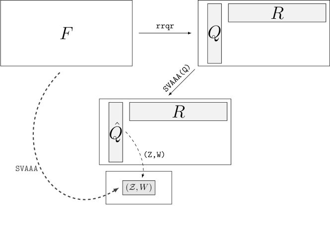
what we have shown in this section can be summarized in the diagram shown in Figure 1. We formalize this in theorem 3.7.

Figure 1: Diagram of the different approximations outlined in Section 3.

Theorem 3.7.

Suppose $Q$ is an orthogonal matrix and $\|F-QC\|_{2}<\epsilon$. Suppose in addition that $F$ can be approximated by $\tilde{F}$ such that $\|F-\tilde{F}\|_{p,\infty}<\epsilon$. With the notation from theorem 3.2, if $\hat{Q}$ is constructed as in theorem 3.6 we have that

$$\forall j\in\{1,\ldots,N\}:\|F(:,j)-\hat{F}(:,j)\|_{\infty}<2\epsilon$$

and

$$\forall j\in\{1,\ldots,N\}:\|\tilde{F}(:,j)-\hat{F}(:,j)\|_{\infty}<3\epsilon.$$

Proof.

Supposing that $\|F-QC\|_{2}<\epsilon$, we have, for any $j\in\{1,\ldots,N\}$

$$\|\tilde{F}(:,j)-\hat{F}(:,j)\|_{\infty} \leq\|F(:,j)-\tilde{F}(:,j)\|_{\infty}+\|F(:,j)-QR(:,j)\|_{\infty}+\|QR(:,j)-\hat{F}(:,j)\|_{\infty}$$

$$<\|F(:,j)-\tilde{F}(:,j)\|_{\infty}+2\epsilon$$

$$<3\epsilon$$

by theorem 3.6 (and by assumption). This in fact proves both statements. ∎

Remark 3.8.

It is simple to see that all of the above results, with slight modifications, still hold in the case of a permuted decomposition, i.e.

$$F\Pi\approx QC.$$

4 QR-based set valued AAA

In this section we outline the ingredients for a single-threaded implementation of ‘QR-AAA’, our set-valued AAA algorithm based on the observations from Section 3. The algorithm is in fact just a simple pivoted rank-revealing $QR$-factorization, followed by a weighted set-valued AAA approximation. In Section 5 we will build on this algorithm and outline a parallel set-valued AAA algorithm.

4.1 QR-AAA

In Theorems 3.5 and 3.6 we wrote the low-rank approximation to $F$ as $QC$, with $Q$ orthogonal, with no constraints on the structure of $C$. There is, of course, a natural candidate for the decomposition $F\approx QC$ and that is the rank-revealing QR decomposition (RRQR). In our implementation, this is based on column pivoted Householder QR (see [9, Chapter 5]). For completeness we include a simple version of colum-pivoted Householder RRQR here, in algorithm 1. Given a matrix $F$, it returns factors $(Q,R)$ and a permutation matrix $\Pi$ such that

$$F\Pi=QR.$$

In addition, we have the following properties, which we include without proof:

Lemma 4.1.

At iteration $k$ of algorithm 1 it holds that

$$|R(1,1)|\geq|R(2,2)|\geq\cdots\geq|R(k,k)|$$

and

$$|R(i,i)|>|R(i,j)|$$

for $1\leq i\leq k$ and $i\leq j\leq N$.

In [9, Chapter 5] it is shown that column-pivoted Householder RRQR can be run in $\mathcal{O}(|Z|Nm+m^{3})$.

Input : Matrix $F\in\mathbb{R}^{Z\times N}$

Output : Orthogonal matrix $Q\in\mathbb{R}^{Z\times m}$, upper triangular matrix $R\in\mathbb{R}^{m\times N}$, permutation $\Pi$ of $\{1,\ldots,N\}$

1 $\Pi\leftarrow\emptyset$;

2 $\mathbf{r}\leftarrow(\|F(:,j)\|_{2}^{2})_{j=1}^{N}$;

3 $K\leftarrow\{1,\ldots,N\}$;

4 for $j=1$ to $N$ do

5       $k_{j}=\arg\max_{k\in K}\mathbf{r}(k)$;

6       $r=\mathbf{r}(k_{j})$;

7       if $r<\text{tol}$ then

8             $m\leftarrow j$ ;

9             break;

10            

11       end if

12      $K=K\backslash\{k_{j}\}$;

13       $\Pi\leftarrow[\Pi,k_{j}]$;

14       Compute Householder reflector $H_{j}$ for column $k_{j}$ of $R$;

15       $R\leftarrow H_{j}R$;

16       $\mathbf{r}\leftarrow\mathbf{r}-(|R(j,:)|^{2})_{j=1}^{N}$;

17      

18 end for

19Accumulate $Q\leftarrow H_{1}\cdots H_{m}$;

Algorithm 1 Simple Rank Revealing QR with Householder Reflectors

input : $F\in\mathbb{C}^{Z\times N}$, convergence tolerance tol

output : $(Z,W)\in Z^{m}\times\mathbb{C}^{m}$, supports and weights of sv-aaa,

$R\in\mathbb{C}^{m(m-1)/2}$ representing factor $R$ (optionally: can be omitted)

init : $\mathbf{d}:=\mathbf{0}\in\mathbb{C}^{N}$, $K:=\{1,\ldots,N\}$,

$G:=0\in\mathbb{C}^{S\times N}$, $B:=0\in\mathbb{C}^{S\times N}$

/* Part 1: scale F */

1 for $j=1,\ldots,N$ do

2       $\mathbf{d}(j)\leftarrow\|F(:,j)\|_{\infty}$;

3       if $\mathbf{d}(j)>0$ then

4             $G(:,j)\leftarrow F(:,j)/\|F(:,j)\|_{\infty};$

5       end if

6      

7 end for

/* Part 2: Construct $Q$ and $R$ */

8 $[Q,R]\leftarrow\textbf{RRQR}(G,\text{tol})$;

/* Part 3: Construct $(\hat{Q},Z,W)$ */

9 $\Gamma\leftarrow diag(R)$;

$(\hat{Q},Z,W)\leftarrow\textbf{SV-AAA}(Q\Gamma,\text{tol})$;

Algorithm 2 QR-based sv-aaa (QR-AAA)

The properties in lemma 4.1 enable us to construct and easily interpret a QR-AAA approximation.

Definition 4.2.

Let $\mathbf{f}:\mathbb{C}\to\mathbb{C}^{N}$ be a set-valued function to be approximated by SV-AAA on the grid $Z$. Let $F\in\mathbb{C}^{Z\times N}$ be the corresponding matrix representation as in Definition 2.1. If the column-pivoted rank-revealing QR decomposition of F, with tolerance $\epsilon$, is given as $F\Pi\approx QR$, we say that the QR-AAA approximation of $F$, at precision $\epsilon$, is $\hat{Q}R$, where $\hat{Q}$ is obtained by weighted SV-AAA, with $\Gamma:=\text{diag}(\{R(k,k)\}_{k})$ (see  3.6 and the subsequent remarks).

Figure 2 shows a simple diagram illustrating QR-AAA.

Figure 2: Diagram showing the principle of QR-AAA

In Section 6 we report the remarkable speed-ups attained by QR-AAA.

Remark 4.3.

The idea of using a QR decomposition in approximation algorithms is not new. Typically, the orthogonal bases obtained by the QR decomposition provide additional stability, as in the RBF-QR method (see e.g. [8] and [23]). In fact, it is standard practice to orthogonalize bases of discretized functions using e.g. Gram-Schmidt or the QR decomposition. Nevertheless, our results on the accuracy of set-valued approximation using the truncated QR decomposition (or in fact the more general orthogonal decomposition $F\Pi\approx QC$) seem new, as is the observation of its computational benefits in the context of set-valued approximation.

5 Parallel QR-AAA

While QR-AAA already performs significantly better than SV-AAA for many problems, it is conceivable that for extremely large problems i.e. when $F$ does not fit in memory or the Loewner matrix vectors associated to the set-valued approximation of $Q$ do not fit in cache, the QR-AAA method can still be infeasible. In that case, we can look for methods to exploit today’s increasing parallel computing power. Below, one such method for parallel QR-AAA, which we call PQR-AAA is outlined. The proposed approach is simple. We start by distributing $F=[F_{1},\ldots,F_{p}]$ over $p$ processors. The first two steps each processor $\mu$ takes are obvious:

• Processor $\mu$ computes $F_{\mu}=Q_{\mu}C_{\mu}$.

• Processor $\mu$ constructs $\hat{Q}_{\mu}$, by computing supports and weights $(Z_{\mu},W_{\mu})$.

At this point we have a piece-wise set-valued rational approximant, consisting of $[\hat{Q}_{1}\cdots\hat{Q}_{p}]$. In principle, if data-compactness is our only goal, we could stop here. However, for various applications, such as Compact Rational Krylov (CORK) methods (see [21]), it is important to obtain an overall rational approximation. The next goal therefore is to ‘glue’ these approximations together. Of course, we do not want to re-approximate $[\hat{Q}_{1}\cdots\hat{Q}_{p}]$ over all of $Z$ again. That would be like never having done parallel QR at all! Without loss of generality we will assume for the rest of this section that the degree of rational approximation of each $\hat{Q}_{\mu}$ is $m-1$. Naively, we can take the union $\cup_{\mu}Z_{\mu}$ of selected support points and interpolate/approximate a rational function on this set. This approach suffers from two fundamental problems:

• even in the case of rational interpolation, the set $\cup_{\mu}Z_{\mu}$ has to be extended with some set $Z^{\textnormal{e}}\subset Z$, otherwise the rational interpolation problem is underdetermined

• in the more desirable case of rational approximation, we must very carefully choose such an extension set, since this process may be very ill-conditioned.

This last claim can be clarified as follows. Given some rational function $f$ on $Z$, it is perfectly possible that its rational interpolant or approximant $\hat{f}$ on $Z_{m}^{+}:=(\cup_{\mu}Z_{\mu}\cup Z^{\textnormal{e}})$ satisfies

$$\|f-\hat{f}\|_{Z_{m}^{+},\infty}<\epsilon$$

while $\|f-\hat{f}\|_{Z,\infty}$ can be ‘exponentially large’, i.e. bound only by $C^{m}\epsilon$ for some large $C$. Currently, no theory to solve this problem for general $Z\subset\mathbb{C}$ exists. However, for the important case of $Z$ a finely sampled equispaced set of points in an interval $[-1,1]$ (which can be adapted to $[a,b]$ and even $\imath[a,b]$) we observe in our experiments that simply adding points sampled uniformly at random from $Z\,\backslash(\cup_{\mu}Z_{\mu})$ results in a satisfactory final accuracy. In essence, the points added can be viewed as a validation set for the final rational approximation.
It is possible to be more deliberate in the selection of $Z^{e}$. We use the theory from [1] for bounded polynomial growth. First we fix some definitions.

Definition 5.1.

Given set-valued AAA approximations $\{\hat{Q}_{\mu}\}_{\mu=1}^{p}$ defined by support points and weights $\{(Z_{\mu},W_{\mu})\}_{\mu=1}^{p}$, we set

$$m^{+}:=2\left|\cup_{\mu=1}^{p}Z_{\mu}\right|-2.$$

Furthermore, for any (ordered) distribution of points $Z^{\textnormal{e}}=\{z_{i}\}_{i=1}^{M}$ in $[-1,1]$, define

$$\zeta(Z^{\textnormal{e}}):=\max_{i}\int_{z_{i}}^{z_{i+1}}\frac{1}{\sqrt{1-x^{2}}}\mathop{}\!\mathrm{d}x.$$

We say that $Z^{\textnormal{e}}\subset Z$ is a good extension set for degree $m^{+}$ if $m^{+}\zeta(Z^{\textnormal{e}})=\gamma$ with $0<\gamma<1$ sufficiently small. Additionally, if we set

$$Z^{+}_{m}:=\left(\cup_{\mu}Z_{\mu}\right)\cup Z^{\textnormal{e}}$$ (13)

we define

$$Q_{1}\uplus\cdots\uplus Q_{p}:=[Q_{1}(Z^{+}_{m},:)\cdots Q_{p}(Z^{+}_{m},:)]$$

where the dependence of $Z^{+}_{m}$ on $Z^{\textnormal{e}}$ is assumed known from context.

As shown in [1], if $\gamma<1$ we have that

$$B(Z^{\textnormal{e}},m^{+}):=\sup_{p\in\mathbb{P}_{m^{+}}}\{\|p\|_{\infty,[-1,1]}\,|\,\|p\|_{\infty,Z^{\textnormal{e}}}\leq 1\}$$ (14)

is bound by

$$B(Z^{\textnormal{e}},m^{+})<\frac{1}{1-\gamma}.$$

Example 5.2.

Given an equispaced grid $Z$ in $[-1,1]$, the mock Chebyshev points (see [5]) of cardinality $M$, denoted by $Z_{\text{cheb},M}$ are the $M$ points in $Z$ closest to the Chebyshev nodes of order $M$. For $|Z|=\mathcal{O}(M^{2})$ (see [1]), the mock Chebyshev points achieve $\zeta\approx\frac{\pi}{M}$. In fact, we can use this to characterize what we mean by a ‘sufficiently fine’ equispaced grid. We can say that $Z$ is ‘sufficiently fine’ with respect to $M$ if the mock Chebyshev points in $Z$ achieve $\zeta(Z_{\text{cheb},M})=\frac{\pi}{M}(1+\delta)$, with $0<\delta<1$ sufficently small. In that case we have, if $M=\lceil 3\pi m^{+}\rceil$, that

$$\frac{1}{1-\gamma}<\frac{1}{1-\frac{1+\delta}{3}}=\frac{3}{2-\delta}<3$$

from which

$$B(Z_{\text{cheb},M},m^{+})<3$$

follows.

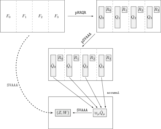
With equation (14) in mind we now have Theorem 5.3, which guarantees satisfactory approximation of the final PQR-AAA step, which we call the accumulate step:

• each node $\mu$ extends its approximation to $\cup_{\mu}Z_{\mu}$

• a final SV-AAA step on $\uplus_{\mu}Q_{\mu}$ is applied.

Theorem 5.3.

We use the notation from Definition 5.1. Suppose $f:=n/d=p/q$ is a rational function on $[-1,1]$ of degree $m-1$, defined by support points and weights $(Z_{m},W_{m})$. Then if $Z_{m}^{+}=Z_{m}\cup Z^{\textnormal{e}}$, we have that any AAA approximant $\hat{f}=\hat{n}/\hat{d}=\hat{p}/\hat{q}$ of degree at most $m-1$ such that

$$\|\hat{d}f-\hat{n}\|_{Z_{m}^{+},\infty}<\epsilon$$ (15)

satisfies

$$\|p\hat{q}-\hat{p}q\|_{\infty,[-1,1]}<\|q\|_{[1,-1],\infty}\|\hat{\ell}\|_{[1,-1],\infty}B(Z^{\textnormal{e}},m^{+})\epsilon$$

where $\hat{\ell}$, as in Equation (1), is the node polynomial for $\hat{f}$.

Proof.

Clearly $p\hat{q}-\hat{p}q$ is a polynomial of degree at most $m^{+}$. It holds that

$$\|p\hat{q}-\hat{p}q\|_{Z_{m}^{+},\infty} =\|q\hat{\ell}(f\hat{d}-\hat{n})\|_{Z_{m}^{+},\infty}$$

$$<\|q\hat{\ell}\|_{\infty,Z_{m}^{+}}\epsilon$$

from which

$$\|p\hat{q}-\hat{p}q\|_{\infty,[-1,1]}<\|q\|_{\infty,Z_{m}^{+}}\|\hat{\ell}\|_{\infty,Z_{m}^{+}}B(Z^{\textnormal{e}},m^{+})\epsilon$$

follows by definition of $B(Z^{\textnormal{e}},m^{+})$ and $Z_{m}^{+}$. ∎

Remark 5.4.

The factor $\|q\|_{\infty,Z_{m}^{+}}<\|q\|_{\infty,[-1,1]}$ serves to make the error relative, since we can arbitrarily rescale the numerator and denominator of $f$ by a common factor. The factor $\|\hat{\ell}\|_{\infty,Z^{+}_{m}}$ is more difficult to analyze. It expresses the maximal size of the node polynomial for the denominator of $\hat{f}$. In principle, it is bounded only by $2^{k}$, for $k-1\leq m-1$ the degree of $\hat{f}$. In practice this growth is rarely observed. In fact, it is possible to explicitely compute $\|\hat{l}\|_{\infty,Z^{+}_{m}}$ in $\mathcal{O}(|Z^{+}_{M}|)$ FLOP at each iteration and incorporating this factor into the convergence criterion for the approximation of $f$ by $\hat{f}$. It should also be noted that the linearized error $\|p\hat{q}-\hat{p}q\|_{\infty,[-1,1]}$ is often a good indicator of the actual error $\|f-\hat{f}\|_{\infty,[-1,1]}$, even though this theoretically only holds if $f$ and $\hat{f}$ have no poles close to, or clustering towards $[-1,1]$. For these cases, a more refined analysis is needed.

A schematic overview of PQR-AAA is given in Figure 3. The attentive reader will have spotted that there is still an all-to-all communication step involved in the accumulation step. While currently we do not know if an all-to-all communication step for the construction of $\cup_{\mu}Z_{\mu}$ (which involves the all-to-all communication of indices) can be avoided, it is possible to avoid the more costly all-to-all communication of blocks $Q(Z_{m}^{+},:)$, by e.g. accumulating the computational nodes two-by-two, as shown in Figure 4.

Figure 3: Illustration of the parallel QR based set-valued AAA approach.

Figure 4: Diagram illustrating the PQR-AAA pairwise accumulation stage. At each stage the ‘$\uplus$’ sum $\hat{Q}_{\mu_{1}}\uplus\hat{Q}_{\mu_{2}}$ of the approximations in two nodes is constructed, after which SV-AAA$(\hat{Q}_{\mu_{1}}\uplus\hat{Q}_{\mu_{2}})$ is computed.

6 Experiments

In this section we demonstrate the effectiveness of QR-AAA and PQR-AAA for some standard matrix functions, as well as on a discontinuous Galerkin BEM system. We illustrate its convergence properties and complexity.

6.1 NLEVP problems

In [3] and [13], a class of reference Non-Linear Eigenvalue Problems (NLEVPs) was introduced, that can serve as a rich source of matrix functions. The matrix functions in the NLEVP benchmark set, available at see [4] are all in split form, meaning

$$F(z)=\sum_{\ell=1}^{L}g(z)M_{\ell}$$

for some set of (typically sparse) matrices $\{M_{i}\}_{\ell=1}^{L}$, and scalar functions $\{g_{i}\}_{\ell=1}^{L}$.
We briefly introduce the NLEVPs we use to test our method, after which we report the performace of QR-AAA. We will not go into too much detail about the structure and properties of the systems. More detailed information about sparsity, eigenvalue distributions, positive (semi-)definiteness of the factors etc. can be found in the NLEVP repository (see [4]).

6.1.1 Problem 1: A Clamped Sandwich Beam

One typical class of NLEVPs come from mechanical systems with nonlinear damping i.e.

$$F(s)=s^{2}M+g(s)D+K$$

with $s\in\imath\mathbb{R}$ the Laplace variable, and $M,D,K$ the Mass, Damping and Stiffness matrices from a FEM discretization of mechanical system, and $g(s)$ some rational function, usually obtained directly in the Laplace domain. We are interested in the case $s\in\imath\mathbb{R}$, as it leads to transfer function approximation. The example of this class we chose is that of the clamped sandwich beam (see [20]). In this problem, the systems are obtained by a FEM discretization of a composite beam with a viscoelastic core, which provides nonlinear damping. The resulting system in the Laplace domain is given by

$$F(s)=\left(K+\frac{G_{0}+(s\tau)^{p}G_{\infty}}{1+(s\tau)^{p}}D+s^{2}M\right)$$

with a fractional parameter $p=.675$, and constants $G_{0},G_{\infty},\tau\in\mathbb{R}$ equal to $350.4\,$kPa, $3.062\,$MPa and $8.230\,$ns respectively. These values are determined experimentally.
We discretize this problem with an equispaced grid $Z\subset[200\imath,30000\imath]$ of size $|Z|=1000$. We run SV-AAA and QR-AAA with the $p=\infty$ error criterion and tolerance $10^{\smin 8}$.

6.1.2 Problem 2: Photonic Crystals

The second problem we consider originates from a 2D Helmholtz problem for Transversely Polarized EM waves on photonic crystals in a medium with frequency-dependent relative permittivity. Discontinuous Galerkin FEM discretization of the differential form of the Helmholtz equation is applied. This results in a rational eigenvalue problem with system

$$F(s)=G+s^{2}(\epsilon_{0}M_{0}+\epsilon_{1}(s)M_{1})$$

where $\epsilon_{0}\in\mathbb{R}$ and

$$\epsilon_{1}(s)=c+\sum_{\ell=1}^{L}\frac{\lambda_{P,\ell}^{2}}{s^{2}+\gamma s+\lambda_{0,\ell}^{2}}$$

with parameters $\gamma,c,\{\lambda_{P,\ell},\lambda_{0,\ell}\}_{\ell}$ in $\mathbb{R}$. Typically, the number of terms $L$ is relatively small. The default value for $L$ in the NLEVP problem set is $2$. Again we are interested in the case $s\in\imath\mathbb{R}$, though in this case this is because it then corresponds to $s=\imath\kappa$, with $\kappa$ the wave number.
We discretize this problem with an equispaced grid $Z\subset[0,10\imath]$ of size $|Z|=1000$. We run SV-AAA and QR-AAA with the $p=\infty$ error criterion and tolerance $10^{\smin 8}$.

6.1.3 Problem 3: Schrödinger’s Equation in a Canyon Well

Our third example comes from the Schrödinger equation for a particle in a canyon-shaped potential well. The particle’s mass has a default value of $0.2\,$me, but can be changed by the user. The measurements of the potential well can be changed as well, but we use the default parameters of the NLEVP benchmark set. The Schrödinger equation is then discretized on a nanometer scale grid, which we will study at various refinements. A more detailed description can be found in [22]. The resulting system has the form

$$F(\lambda)=H-\lambda\mathds{1}-\sum_{\ell=1}^{L}e^{\imath\sqrt{m(\lambda-a_{\ell}})}S_{\ell}$$

where for each $\ell$, the matrix $S_{\ell}$ is sparse and of rank 2. We have switched from the Laplace variable $s$ to a real variable $\lambda$ here. The values $\{a_{\ell}\}_{\ell}$ are branch points on the real axis. The number of terms $L$ for the nonlinear part is quite large, compared to the previous two examples: it is equal to $81$ by default!
We discretize this problem with an equispaced grid $Z\subset[p_{1},p_{2}]$ of size $|Z|=1000$. We run SV-AAA and QR-AAA with the $p=\infty$ error criterion and tolerance $10^{\smin 8}$.

6.1.4 Problem 4: Time Delay Systems with random delays

The Laplace transform of a time delay system has the form

$$F(s)=s\mathds{1}-\sum_{\ell=1}^{L}A_{\ell}e^{-s\tau_{\ell}}$$

with $\{A_{\ell}\}_{\ell}$ typically dense matrices representing the gain at delay $\tau_{\ell}\in\mathbb{R}^{+}$. We take a sequence of delays $1,2,\ldots,L$ and randomly generated $A_{\ell}$ matrices, of linearly increasing $\|\cdot\|_{\infty}$-norm (here, $\|A_{\ell}\|_{\infty}=10^{\ell/2}$). We set $L=20$. This way, problem $4$ provides an intermediate between the relatively low split degree systems of problem 1 and 2, and the rather high degree system of problem 4. Since the matrices $\{A_{\ell}\}_{\ell}$ are generated randomly, and because of the oscillatory nature of the exponential functions, this is a particulary tough problem for standard rational approximation.
We discretize this problem with an equispaced grid $Z\subset[-10\imath,10\imath]$ of size $|Z|=1000$. We run SV-AAA and QR-AAA with the $p=\infty$ error criterion and tolerance $10^{\smin 4}$. The approximation is run at a lower tolerance because for higher tolerances the memory requirements and computation time become exceedingly large.

6.1.5 Numerical results

In this subsection we present the numerical performance of QR-AAA. We ran our experiments on an 8 core (16 virtual) AMD Ryzen 7 PRO 5850U x86_64 CPU and report the timings and convergence behavior of both QR-AAA and SV-AAA. Each of the $4$ NLEVP problem $F$ matrices is approximated with the specifics stated.
The time (in seconds) needed for the QR approximation of $F$ is denoted by t_QR, while the time for the set-valued AAA approximations for the $Q$ factor and the $F$ matrix are denoted by t_AAA_Q and t_AAA_F respectively. The timings were averaged over 10 experiments each, except for t_AAA_F for the largest instance (at $N=98442$) for problem $4$.
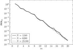
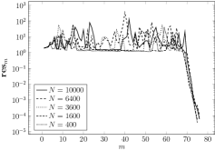
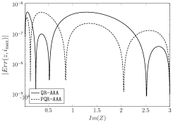
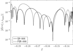
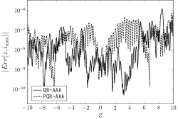
We report the values of the absolute timings for t_QR, t_AAA_Q, t_AAA_F in the tables in Figure 7. When compared to the timings for SV-AAA, the timings for QR-AAA are almost negligible. Only at very large scales, basically when a single column of $Q$ no longer fits in cache, do we even register any cost for the QR decomposition at all. The only exception to this is problem $4$. We clearly see that t_AAA_Q does not increase with increasing $N$, in fact, it often decreases. From the convergence plots in figures 5 and 6, we see why this is; the timings for the set-valued part of QR-AAA depend on the degree of approximation $m$, and the rank of $Q$, but not on $N$. The time t_QR however does increase linearly with $N$, as expected, but since the QR factorization is fundamentally less computationally expensive as the SVD of the large Loewner matrices arising in the direct application of SV-AAA on $F$, we have that $\texttt{t\_QR}\ll\texttt{t\_AAA\_F}$.
Finally, we can also see from figures 5 and 6 that the SV-AAA approximation and the QR-AAA approximation are essentially identical. This backs up Theorem 3.6 and 3.7 numerically, and shows that QR-AAA is equivalent to SV-AAA, only much faster.

(a) Problem 1: SV-AAA

(b) Problem 1: QR-AAA

(c) Problem 2: SV-AAA

(d) Problem 2: QR-AAA

Figure 5: Residue $\textbf{res}_{m}$ for SV-AAA (left) and QR-AAA (right) over the rational approximation degree $m$, for the first two selected problems from the NLEVP benchmark set.

(a) Problem 3: SV-AAA

(b) Problem 3: QR-AAA

(c) Problem 4: SV-AAA

(d) Problem 4: QR-AAA

Figure 6: Residue $\textbf{res}_{m}$ for SV-AAA (left) and QR-AAA (right) over the rational approximation degree $m$, for the second two selected problems from the NLEVP benchmark set.

$N$	t_QR	t_AAA_Q	t_AAA_F
$1240$	$0.025$	$4.02\mathrm{e}{-3}$	$1.93$
$6280$	$0.124$	$2.24\mathrm{e}{-3}$	$6.04$
$25180$	$0.470$	$1.63\mathrm{e}{-3}$	$20.41$

(a) Problem 1

$N$	t_QR	t_AAA_Q	t_AAA_F
$5546$	$0.108$	$5.56\mathrm{e}{-3}$	$2.61122$
$29034$	$0.527$	$1.26\mathrm{e}{-3}$	$13.7263$
$98442$	$1.756$	$1.14\mathrm{e}{-3}$	$54.847$

(b) Problem 2

$N$	t_QR	t_AAA_Q	t_AAA_F
$5971$	$0.278$	$8.351\mathrm{e}{-2}$	$70.4021$
$7432$	$0.381$	$8.39\mathrm{e}{-2}$	$86.9885$
$10157$	$0.447$	$8.32\mathrm{e}{-2}$	$119.217$
$15121$	$0.683$	$8.38\mathrm{e}{-2}$	$177.209$

(c) Problem 3

$N$	t_QR	t_AAA_Q	t_AAA_F
$400$	$0.010$	$9.21$	$232.38$
$1600$	$0.091$	$9.41$	$1033.47$
$3600$	$0.241$	$9.51$	$2285.06$
$6400$	$0.440$	$9.67$	$4431.65$
$10000$	$0.701$	$9.41$	$6370.27$

(d) Problem 4

Figure 7: Tables of absolute timings for SV-AAA and QR-AAA, for the four NLEVP problems. All timings are reported in seconds.

Figure 8: Error plots over the matrix parameter of QR-AAA (full) and PQR-AAA (dashed)

7 BEM near-field compression using PQR-AAA

In the discontinuous Galerkin boundary element method for the Helmholtz equation (see e.g. [18]), boundary integral operators are discretized using finite-dimensional ansatz spaces and testspaces. The simplest such boundary integral operator, the single layer boundary operator, is defined by

$$\mathcal{S}:H^{-1/2}(\partial\Omega)\to H^{1/2}(\partial\Omega):u\mapsto\mathcal{S}u$$

where

$$(\mathcal{S}u)(\mathbf{x})=\lim_{\mathbf{x}\to\partial\Omega}\int_{\partial\Omega}G(\mathbf{x},\mathbf{y};\kappa)u(\mathbf{y})dS_{\mathbf{y}}$$

with $G(\mathbf{x},\mathbf{y};\kappa)$ the Green’s kernel for the Helmholtz equation at wave number $\kappa$.
Using a triangular mesh $\Gamma\approx\partial\Omega$ consisting of $N_{t}$ triangles and the space of piecewise discontinuous linear functions

$$V^{1,{-}1}_{\Gamma}=\text{span}\{\phi_{i}^{\ell}\,|\,(i,\ell)\in\{1,\ldots,N_{t}\}\times\{1,2,3\}\}$$

spanned by the piecewise linear degrees-of-freedom defined on the mesh triangles of $\Gamma$, the operator equation

$$\mathcal{S}u=g$$

is discretized to

$$S^{1,{-}1}\mathbf{u}=\mathbf{g}$$

where $\mathbf{u},\mathbf{g}\in\mathbb{C}^{3N_{t}}$. and

$$S^{1,{-}1}(i,\ell_{1};j,\ell_{2})=\langle\mathcal{S}\varphi_{i}^{\ell_{1}},\varphi_{j}^{\ell_{2}}\rangle$$ (16)

These integrals become (weakly) singular when mesh triangles touch or overlap. More generally, the near-field of $S^{1,{-}1}$ consists, roughly speaking, of the blocks of $S^{1,{-}1}$ which correspond to small clusters of $\Gamma$ that are considered close to each other. See [12] for more details. In the nearfield, often specialized singular quadrature schemes must be used in the case of triangles with common vertices (see [18]) or tensor quadrature of high degree must be used to ensure a sufficient accuracy for the case of mesh triangles that are close together.
To demonstrate the power of the PQR-AAA approach we apply it to the compression of the near-field of $S^{1,{-}1}$ as it varies over the wave number. This is an important task, as approximation the wavenumber dependence then allows us to avoid the costly evaluation of the $4D$ singular integrals arising in the numerical evaluation of equation (16). The matrix $F$ from Definition 2.1 in this case has columns corresponding to $S^{1,\smin 1}(i,\ell_{1};j,\ell_{2};Z)$, where $(i,\ell_{1};j,\ell_{2})$ ranges over the near-field DOFs, and $Z\subset[\kappa_{\min},\kappa_{\max}]$ is a discrete, sufficiently fine subset of the selected frequency range. For our experiment, we set $\Gamma$ to be a spherical grid obtained from a $6$-fold spherical refinement of an octahedral mesh. We collect the near-field varying over the wave-number in $F$ and apply PQR-AAA to it (after proper re-scaling of the columns of $F$). We ran our experiment over 28 cores. The total number of functions to be approximated is $1000000$, which are distributed (roughly) equally among the 28 cores. The required tolerance was set to $10^{\smin 6}$. The (dimensionless) wavenumber range was set to $[1.,80.]$, and discretized into $500$ equispaced points. The timings are split up into three constituents:

• t_F: the maximal time needed to assemble the matrix $F_{mu}$, over the processors $\mu\in\{1,\ldots,28\}$,

• t_QR: maximal time needed to compute the approximate pivoted Householder QR decomposition $F_{\mu}\approx Q_{\mu}R_{\mu}$ over the processors $\mu\in\{1,\ldots,28\}$,

• t_AAA_Q: the maximal time needed to compute the SV-AAA approximation of $Q_{\mu}$ over the processors $\mu\in\{1,\ldots,28\}$.

• t_fin: the time needed to compute the final SV-AAA for $\uplus_{\mu}Q_{\mu}$

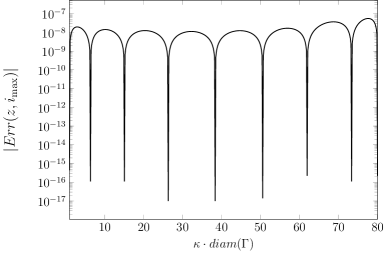
These timings, as well as the supremum norm error over $F$, are reported for our set-up in table 1. The error over the wavenumber of the final approximation is reported in Figure 9. As can be seen from this figure, the final degree of rational approximation is $12$. The maximum error of the final approximant is well below the requested tolerance. Recall that, because of the scaling of the columns in $F$, this error is relative.

t_F	t_QR	t_AAA_Q	t_fin	$\textbf{Err}_{\infty}(F)$
$343.213$	$.926$	$.019$	$.259$	$6.64897\cdot 10^{-8}$

Table 1: Supremum norm error and components of the PQR-AAA timings (in s) for the the near-field of $S^{1,\smin 1}_{\mathcal{H}}$ defined on the sphere $S^{2}$.

Figure 9: Error near-field

References

- [1] Adcock, B., Platte, R. B., and Shadrin, A. Optimal sampling rates for approximating analytic functions from pointwise samples. IMA J. Numer. Anal. 39, 3 (2018), 1360–1390.
- [2] Antoulas, A. C., and Anderson, B. D. Q. On the scalar rational interpolation problem. IMA J. Math. Contr. Inf. 3, 2 (1986), 61–88.
- [3] Betcke, T., Higham, N. J., Mehrmann, V., Schröder, C., and Tisseur, F. NLEVP: A collection of nonlinear eigenvalue problems. ACM Trans. Math. Softw. 39, 2 (2013), 1–28.
- [4] Betcke, T., Higham, N. J., Mehrmann, V., Schröder, C., and Tisseur, F. NLEVP: A collection of nonlinear eigenvalue problems. https://www.github.com/ftisseur/nlevp, 2013.
- [5] Boyd, J. P., and Xu, F. Divergence (Runge phenomenon) for least-squares polynomial approximation on an equispaced grid and mock Chebyshev subset interpolation. Appl. Math. Comput. 210, 1 (2009), 158–168.
- [6] Dirckx, S., Huybrechs, D., and Meerbergen, K. Frequency extraction for BEM matrices arising from the 3D scalar Helmholtz equation. SIAM J. Sci. Comput. 44, 5 (2022), B1282–B1311.
- [7] El-Guide, M., Miȩdlar, A., and Saad, Y. A rational approximation method for solving acoustic nonlinear eigenvalue problems. Eng Anal Bound Elem 111 (2020), 44–54.
- [8] Fornberg, B., Larsson, E., and Flyer, N. Stable computations with Gaussian radial basis functions. SIAM Journal on Scientific Computing 33, 2 (2011), 869–892.
- [9] Golub, G. H., and van Loan, C. F. Matrix Computations, Fourth ed. JHU Press, 2013.
- [10] Güttel, S., Negri Porzio, G. M., and Tisseur, F. Robust rational approximations of nonlinear eigenvalue problems. SIAM J. Sci. Comput. 44, 4 (2022), A2439–A2463.
- [11] Güttel, S., Van Beeumen, R., Meerbergen, K., and Michiels, W. NLEIGS: A class of fully rational Krylov methods for nonlinear eigenvalue problems. SIAM J. Sci. Comput. 36 (2014), A2842–A2864.
- [12] Hackbusch, W. Hierarchical Matrices: Algorithms and Analysis. Springer Series in Computational Mathematics. Springer-Verlag, Berlin-Heidelberg, 2010.
- [13] Higham, N. J., Porzio, G. M. N., and Tisseur, F. An updated set of nonlinear eigenvalue problems. Available at https://api.semanticscholar.org/CorpusID:164833102, 2019.
- [14] Hochman, A. FastAAA: A fast rational-function fitter. In 2017 IEEE 26th Conference on Electrical Performance of Electronic Packaging and Systems (EPEPS) (2017), pp. 1–3.
- [15] Huybrechs, D., and Trefethen, L. N. AAA interpolation of equispaced data. BIT 63 (2023), 1–19.
- [16] Lietaert, P., Meerbergen, K., Pérez, J., and Vandereycken, B. Automatic rational approximation and linearization of nonlinear eigenvalue problems. IMA J. Numer. Anal. 42, 2 (2022), 1087–1115.
- [17] Nakatsukasa, Y., Sète, O., and Trefethen, L. N. The AAA algorithm for rational approximation. SIAM J. Sci. Comput. 40, 3 (2018), A1494–A1522.
- [18] Sauter, S., and Schwab, C. Boundary Element Methods, vol. 39 of Springer Series in Computational Mathematics. Springer, Berlin, 2011.
- [19] Su, Y., and Bai, Z. Solving rational eigenvalue problems via linearization. SIAM J. Matrix Anal. Appl. 32, 1 (2011), 201–216.
- [20] Van Beeumen, R., Meerbergen, K., and Michiels, W. A rational Krylov method based on Hermite interpolation for nonlinear eigenvalue problems. SIAM J. Sci. Comput. 35, 1 (2013), A327–A350.
- [21] Van Beeumen, R., Meerbergen, K., and Michiels, W. Compact rational Krylov methods for nonlinear eigenvalue problems. SIAM J. Matrix Anal. Appl. 36 (2015), 820–838.
- [22] Vandenberghe, W., Fischetti, M., Van Beeumen, R., Meerbergen, K., Michiels, W., and Effenberger, C. Determining bound states in a semiconductor device with contacts using a nonlinear eigenvalue solver. J. Comput. Electron. 13 (07 2014), 753–762.
- [23] Wright, G. B., and Fornberg, B. Stable computations with flat radial basis functions using vector-valued rational approximations. JCP 331 (2017), 137–156.