The Physics-Informed Neural Network Gravity Model Generation III

Abstract

Scientific machine learning and the advent of the Physics-Informed Neural Network (PINN) show considerable potential in their capacity to identify solutions to complex differential equations. Over the past two years, much work has gone into the development of PINNs capable of solving the gravity field modeling problem — i.e. learning a differentiable form of the gravitational potential from position and acceleration estimates. While the past PINN gravity models (PINN-GMs) have demonstrated advantages in model compactness, robustness to noise, and sample efficiency; there remain key modeling challenges which this paper aims to address. Specifically, this paper introduces the third generation of the Physics-Informed Neural Network Gravity Model (PINN-GM-III) which solves the problems of extrapolation error, bias towards low-altitude samples, numerical instability at high-altitudes, and compliant boundary conditions through numerous modifications to the model’s design. The PINN-GM-III is tested by modeling a known heterogeneous density asteroid, and its performance is evaluated using seven core metrics which showcases its strengths against its predecessors and other analytic and numerical gravity models.

1 Introduction

Nearly all problems in astrodynamics involve the force of gravity. Be it in celestial mechanics, trajectory optimization, spacecraft rendezvous, space situational awareness, or other problems, gravity often plays a significant — if not dominant — role in the system dynamics. The mere ubiquity of this force is a testament to its significance, yet despite this, there exist surprisingly few ways to represent this force to high accuracy. The construction of high-fidelity gravity models is henceforth referred to as the gravity modeling problem, and currently there exists no universal solution. Some gravity models perform well for large planetary bodies, but break down when modeling objects with exotic shapes like asteroids and comets. Other models can handle irregular geometries but require assumptions and come with high computational cost. At its core, all current gravity models come with unique pitfalls that prevent standardization across the community. Consequently, researchers are exploring alternative strategies to solve the gravity modeling problem in the hopes of finding a universal model. One encouraging vein of research explores the use of neural networks and scientific machine learning to circumvent many of these past difficulties.

Figure 1: PINN-GMs offer high-accuracy, low-cost gravity solutions to be deployed across a variety of use cases and applications.

Scientific machine learning proposes the use of neural networks to learn high-fidelity models of, and solutions to, complex differential equations cuomoScientificMachineLearning2022 ; karniadakisPhysicsinformedMachineLearning2021 . Physics-informed neural networks (PINNs) are one class of model available to solve such problems. PINNs are neural networks specifically trained to represent a solution to a differential equation in a way that respects relevant differential and physics-based constraints. This compliance, or “physics-informing”, is achieved by augmenting the network cost function with these differential constraints, such that the learned model is penalized for violating any of the underlying physics. Through this design change, PINNs have been shown to achieve higher accuracy with less data than their traditional neural network counterparts raissiPhysicsinformedNeuralNetworks2019 .

Recently, researchers have begun to explore the use of PINNs to solve the gravity modeling problem martinEarthAndMoon2022 ; martinSmallBodies2022 . These models, referred to as PINN gravity models (PINN-GMs), have demonstrated considerable promise in their ability to learn high-fidelity gravity models from sparse and noisy data in both large and small-body settings. Despite their preliminary success, these models have also demonstrated a number of shortcomings which this paper aims to address. Specifically, this paper introduces the third generation of the PINN-GM (PINN-GM-III) which solves the problems of extrapolation error, numerical instability, bias towards low-altitude samples, and compliant boundary conditions through numerous modifications to the model’s design.

2 Background

There exist two families of gravity models: analytic and numerical. Analytic models are derived from first principles like Laplace’s equation, whereas numerical models are constructed in a data-driven manner. Each model has its own set of advantages and drawbacks, and the choice of which model to use is often dictated by the application. The following section details the available gravity models and their respective pros and cons.

2.1 Spherical Harmonics Model

Early in the 1900s, it was proposed that spherical harmonic basis functions could be superimposed to produce a high-fidelity estimate of the gravitational potential brillouinEquationsAuxDerivees1933 :

$$U(r)=\frac{\mu}{r}\sum_{l=0}^{l}\sum_{m=0}^{l}\bigg{(}\frac{R}{r}\bigg{)}^{l}P_{l,m}\left(\sin\phi\right)\big{[}C_{l,m}\cos(m\lambda)+S_{l,m}\sin(m\lambda)\big{]}$$ (1)

Equation (1) is referred to as the spherical harmonic gravity model where $r$ is the distance to the field point, $\mu$ is the gravitational parameter of the body, $R$ is the circumscribing radius of the body, $l$ is the degree of the model, $m$ is the order of the model, $C_{l,m}$ and $S_{l,m}$ are the Stokes coefficients, $\lambda$ is the longitude, $\phi$ is the latitude, and $P_{l,m}$ are the associated Legendre polynomials kaulaTheorySatelliteGeodesy1966 .

The spherical harmonic gravity model is the primary model of choice to represent the gravity fields of large planetary bodies like the Earth pavlisPreliminaryGravitationalModel2005 , Moon goossensGlobalDegreeOrder2016 , and Mars genovaSeasonalStaticGravity2016a . One of the most compelling advantages of the spherical harmonic gravity model is how it can compactly capture one of the largest gravitational perturbations: planetary oblateness. Because the Earth and these other large bodies rotate about their axes, a centrifugal acceleration is produced which flattens the body from a sphere into an oblate ellipsoid gravityEarthGravitationalField2016 . This flattening or excess of mass near the equator is referred to as planetary oblateness, and its presence has sizable effects on spacecraft trajectories. It is therefore important that this perturbation is accurately captured in a gravity model. The spherical harmonic gravity model makes this simple, needing only one harmonic in the expansion to capture this oblateness ($C_{2,0}$, or its alternative form $J_{2}=-C_{2,0}$).

While spherical harmonics are effective at representing planetary oblateness, they struggle to model the remaining and more discrete gravitational perturbations like mountain ranges, tectonic plate boundaries, and craters. Discontinuities are notoriously difficult to represent using periodic basis functions, often requiring hundreds of thousands of harmonics being superimposed to overcome the 3D equivalent of Gibbs phenomena hewittGibbsWilbrahamPhenomenonEpisode1979 . Not only must these harmonics be superimposed, they must be regressed, and the high-frequency signals become increasingly difficult to detect due to their fading observability from the $(R/r)^{l}$ term in Equation (1). Taken together, these conditions results in large, memory inefficient models that become challenging to keep on-board spacecraft. In addition, these high-fidelity models can carry a hefty computational cost, as all associated Legendre polynomials must be reevaluated at each field point. These calculations are recursive and therefore cannot be parallelized, leading to an unavoidable $\mathcal{O}(n^{2})$ computational complexity which can severely limit both ground-based simulation and algorithms flown on-board martinGPGPUImplementationPines2020 .

Beyond the computational inefficiencies, spherical harmonics also has operational limits. The derivation of this model requires that all mass elements exist within a sphere of fixed radius (the Brillouin radius). If dynamicists require a potential or acceleration estimate within this sphere, the model risks diverging from the $(R/r)^{l}$ term in the expansion. While such effects are negligible for near-spherical planets or moons, they can become problematic in small-body settings. For asteroids or comets that exhibit highly non-spherical geometries like Eros or Itokawa, these effects can lead to large errors in the predicted accelerations and potentially risk the safety of spacecraft wernerExteriorGravitationPolyhedron1997 .

2.2 Polyhedral Gravity Model

The polyhedral gravity model provides an alternative to the spherical harmonic model in these settings, offering a solution that maintains validity down to the surface of any body regardless of shape. This stability makes the polyhedral model especially popular for exploration about small-bodies such as asteroids and comets. If a shape model of the body is available — a collection of triangular facets and vertices which captures the geometry of the object — then the associated gravitational potential of that geometry can be computed under the assumption of constant density through:

$$\nabla U=-G\sigma\sum_{e\in\text{edges}}\mathbf{E}_{e}\cdot\mathbf{r}_{e}\cdot L_{e}+G\sigma\sum_{f\in\text{facets}}\mathbf{F}_{f}\cdot\mathbf{r}_{f}\cdot\omega_{f}$$ (2)

where $G$ is the gravitational constant, $\sigma$ is the density of the body, $\mathbf{E}_{e}$ is an edge dyad, $\mathbf{r}_{e}$ is the position vector between the center of the edge and the field point, $L_{e}$ is an analog to the potential contribution by the edge, $\mathbf{F}_{f}$ is the face normal dyad, $\mathbf{r}_{f}$ is the distance between the face normal and the field point, and $\omega_{f}$ is an analog to the potential contribution by the face wernerExteriorGravitationPolyhedron1997 .

While the polyhedral gravity model circumvents the numerical divergence within the Brillouin sphere, it comes with its own unique disadvantages. Foremost, this gravity model can be computationally expensive. High-resolution shape models have hundreds of thousands of facets and vertices which must be individually looped over to compute the acceleration at a single field point. When computing many accelerations or propagating trajectories, this computational burden can lead to excessively long runtimes. While this model can take advantage of parallelization more easily than spherical harmonics, such computational capabilities are not available on-board spacecraft — intrinsically limiting this model to ground-based simulation.

Another disadvantage of the polyhedral gravity model comes in the form of its assumptions. The model assumes that researchers know a density profile for the body in question. Most commonly the density is assumed to be constant, but literature shows that such assumption is not necessarily valid scheeresEstimatingAsteroidDensity2000 ; scheeresHeterogeneousMassDistribution2020 . In addition, the polyhedral gravity model assumes that shape model of the body already exists. While these models can be acquired in-situ, the process is non-trivial and time-consuming in practice zuberShape433Eros2000 ; shepardRevisedShapeModel2018 ; millerDeterminationShapeGravity2002 .

2.3 Other Analytic Models

Additional analytic models have been proposed which attempt to bypass some of the challenges faced by the popular spherical harmonic and polyhedral models. The ellipsoidal harmonic model follows a similar approach to that of spherical harmonics but uses ellipsoidal harmonic basis functions instead romainEllipsoidalHarmonicExpansions2001 . This choice allows for a tighter bounding ellipsoid about the body than spherical harmonics, minimizing the region in which the model could potentially diverge. Despite this, the divergence remains a possibility inside the bounding ellipsoid and the model still suffers from the same challenges in representing discontinuity with periodic basis functions.

Alternatively, the interior spherical harmonic model inverts the classical spherical harmonic formulation and can model a local region whose boundary intersects only one point on the surface of the body takahashiSurfaceGravityFields2013 . This model maintains stability down to that single point making it valuable for precise landing operations; however, the solution becomes invalid on any other point on the surface and outside of the corresponding local sphere. The interior spherical Bessel gravity model expands on this theme, using bessel functions rather than spherical harmonics, and is able to achieve a wider region of validity. However, this comes at the expense of cumbersome analytics and retains some of the challenges of using harmonic basis functions to capture discontinuity takahashiSmallBodySurface2014 .

In contrast to harmonic models, mascon gravity models distribute a set of point mass elements within a body whose sum can form a global representation of the gravity field mullerMasconsLunarMass1968 . Unfortunately, the accelerations can grow inaccurate at field points near the individual mascons tardivelLimitsMasconsApproximation2016 . Hybrid mascon models offer a slightly more robust alternative to the pure mascon approach by representing each mascon with a low fidelity spherical harmonic model, but this incorporates additional complexity in regression and remains prone to both challenges of the mascon and spherical harmonic models wittickMixedmodelGravityRepresentations2019 .

2.4 Traditional Machine Learning Models

As an alternative to the analytic models, recent efforts explore the use of machine learning to learn representations of complex gravity fields in a data-driven manner. In principle, machine learning models can learn high-accuracy gravity fields without making any intrinsic assumptions about the body in question, while maintaining low computational cost.

Model	Parameters	Training Data	Avg. Error [%]	Valid Globally
GP gaoEfficientGravityField2019	12,960,000	3,600	1.5%	✗
NNs chengRealtimeControlFueloptimal2019	1,575,936	800,000	0.35%	✗
ELMsfurfaroModelingIrregularSmall2020	100,000	768,000	1-10%	✗
GeodesyNet izzoGeodesyIrregularSmall2022	91,125	500,000	0.36%	✗
PINN-GM-III	2,211	4,096	0.30%	✓

Table 1: Machine Learning Gravity Model Statistics – See Appendix C

Gaussian Processes

The first proposed effort to use machine learning for the gravity modeling problem was introduced in 2019 and leveraged Gaussian processes to learn a mapping between position and acceleration from a set of training data gaoEfficientGravityField2019 . Gaussian processes are fit by specifying a prior distribution over functions, and updating that prior based on observed data. This requires the user to specify some kernel function which provides a metric of similarity between data, and computing a covariance matrix between all data points using that function. Once the covariance matrix is computed, it can be inverted and used evaluate the mean and covariance of the learned function at a test point.

Using Gaussian processes for gravity modeling is advantageous because it provides a probabilistic estimate of the uncertainty in the model’s prediction; however the model does not scale well to large data sets. Specifically, the Gaussian process is characterized by a covariance matrix built from the training data. This covariance matrix scales as $\mathcal{O}(n^{2})$ where $n$ is the size of the training data. This scaling makes it computationally challenging for Gaussian processes to leverage large quantities of data, as the size of the covariance matrix and complexity of corresponding inversion grows rapidly with small sets of training data. As an example, in Reference 26, a Gaussian process is regressed over a mere 3,600 data points resulting in a model covariance matrix of over 12,960,000 parameters. Because this model size grows rapidly, researchers must carefully select which training data to leverage, and inevitably are unable to model the entire testing domain highlighting an intrinsic limitation of these models. Aside from this fact, the study does demonstrate that these models, once fit, can achieve fast evaluation times and relatively high-accuracy predictions near the training data.

Extreme Learning Machines

Alternatively, extreme learning machines (ELMs) are single layer neural networks which are fit by randomly initializing the weights from the inputs to the hidden layer, and then solving for the weights to the output layer using a least squares approach to minimize some quadratic cost function such as:

$$L(\theta)=\frac{1}{N}\sum_{i=0}^{N}|\hat{\bm{y}}_{i}(\bm{x}_{i}|\theta)-\bm{y}_{i}|^{2}$$ (3)

where $\hat{y}_{i}(\bm{x_{i}}|\theta)$ is the machine learning model prediction at input $\bm{x}_{i}$ with trainable model parameters $\theta$ huangExtremeLearningMachine2006 . The ELM is advantageous over other methods because it can be trained in a single iteration using least squares as opposed to neural networks which require many iterations of stochastic gradient descent and backpropagation. ELMs have been used to learn a mapping between position and acceleration for the asteroid Itokawa and again demonstrate fast evaluation speeds with relatively high accuracy furfaroModelingIrregularSmall2020 . That said, the models require large training datasets ($>$750,000 data), long training times (approximately 40 hours), and its performance is not assessed at high altitudes.

Neural Networks

As an alternative to ELMs, neural networks have also been proposed to learn a gravity model from position and acceleration data chengRealtimeOptimalControl2020 . These models are also trained to minimize a cost function, but do so using some flavor of stochastic gradient descent — iteratively updating the network weights with optimization algorithms like ADAM kingmaAdamMethodStochastic2014 , NADAM dozatIncorporatingNesterovMomentum , LBFGS nocedalNumericalOptimization2006 , etc. The advantages of using a neural network come in their ability to represent highly non-linear functions, but they are traditionally over-parameterized leading to large models that would be challenging to fly directly on-board. Similar to the ELM, the models trained in Reference 31 required a large set of training data ($>$1,000,000 data) and their performance is not assessed at high altitudes.

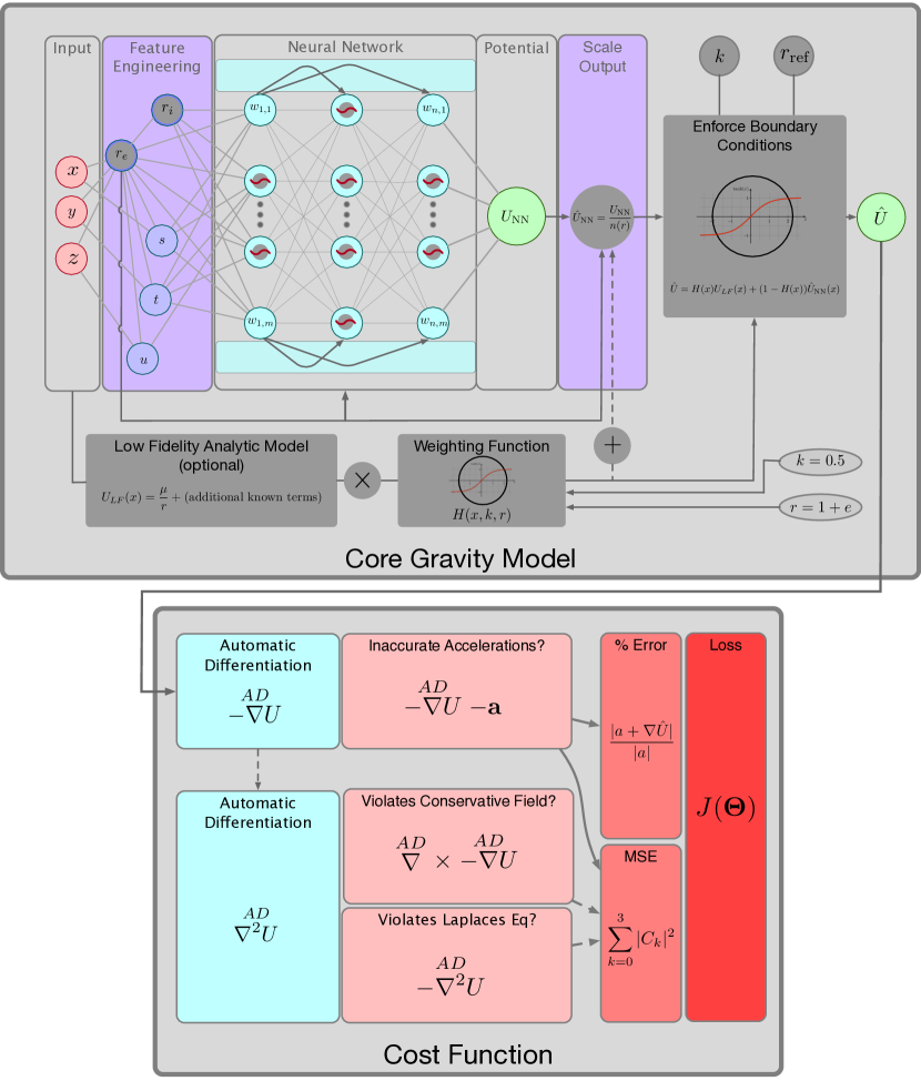
Figure 2: PINN-GM Generation III with new modifications contained in dark gray boxes

GeodesyNet

In 2021, Reference 29 proposed the use of neural density fields to learn density maps for small bodies. This research takes inspiration from recent machine learning developments in Neural Radiance Fields (NeRFs) which are used to construct 3D scenes from relatively sparse image data mildenhallNeRFRepresentingScenes2022 . Once trained, the density predictions can be integrated numerically to produce corresponding gravitational potentials and accelerations. This work demonstrated promising results – achieving competitive acceleration accuracies and the ability to account for heterogeneous densities; however, the models are relatively large (in excess of 90,000 parameters), the numerical integration necessary to compute accelerations is computationally expensive, and the models continued to require large training datasets.

2.5 Physics-Informed Neural Network Gravity Model

As discussed previously, Physics-Informed Neural Networks (PINNs) are a relatively new class of machine learning algorithms which explicitly incorporate known differential constraints into their cost function raissiPhysicsinformedNeuralNetworks2019 . By penalizing violations of these constraints during training, the networks are forced to learn solutions which are naturally compliant with the underlying physics.

In 2022, Reference 4 proposed the Physics-Informed Neural Network Gravity Model (PINN-GM) as a candidate solution to the gravity modeling problem. Rather than training traditional neural networks with a cost function like what is shown in Equation (3), the PINN-GM used a cost function of which leverages the known differential equation $-\nabla U=\bm{a}$ through

$$L(\theta)=\frac{1}{N}\sum_{i=0}^{N}|-\nabla\hat{U}(x_{i}|\theta)-\bm{a}_{i}|^{2}$$ (4)

where $\nabla\hat{U}$ is taken via automatic differentiation of the neural network baydinAutomaticDifferentiationMachine2018 .

Reference 4 explores the utility of this modeling approach as an alternative to spherical harmonics for the cases of the Earth and Moon. The results demonstrate that in some altitude regimes, the PINN-GM can produce acceleration of comparable accuracy to high-fidelity spherical harmonic models using nearly an order of magnitude fewer parameters. Later this work was extended to small-body settings, and additional design modifications were introduced including additional physics constraints, a modified network architecture, and feature engineering to achieve high-fidelity gravity models using order of magnitude smaller sets of data than of past approaches martinSmallBodies2022 .

Despite the promising developments for the PINN gravity model, this work highlights previously unnoticed pitfalls of these models and proposes design changes to address them. Explicitly, this paper introduces the third generation PINN gravity model (PINN-GM-III) which includes multiple design changes aimed at address problems in numerical instability, deteriorating performance at high altitudes, extrapolation error, and more.

3 PINN-GM-III

The third generation PINN gravity model (PINN-GM-III) introduces a collection of new design choices to address various failure points of past generations, while also increasing model accuracy and robustness. An architectural glance of these changes are shown in dark gray in Figure 2. All design modifications are detailed in the subsections below.

Algorithm 1 PINN-GM-III algorithm

1:Collect training data ($\bm{x},\bm{a}$) from:
(a) a pre-existing model
(b) online state estimates martinPINNFilter2022

2:Non-dimensionalize the training data $\ignorespaces\triangleright$ Sec. 3.1

3:Convert to non-singular spherical coordinates ($r_{i}$, $r_{e}$, $s,t,u$) $\ignorespaces\triangleright$ Sec. 3.1

4:Propagate through the neural network

5:Output proxy potential $U_{\text{NN}}$ $\ignorespaces\triangleright$ Sec. 3.3

6:Scale proxy potential into true potential $\hat{U}_{\text{NN}}$ $\ignorespaces\triangleright$ Sec. 3.3

7:(Optional) Fuse with weighted low-fidelity potential $\hat{U}_{\text{LF}}$

8:Enforce boundary conditions on the network potential $\hat{U}$ $\ignorespaces\triangleright$ Sec. 3.4

9:Autodifferentiate (AD) potential to produce acceleration $\hat{\bm{a}}$

10:if Training then

11:    Sum acceleration percent error and RMS to form loss $\ignorespaces\triangleright$ Sec. 3.2

12:    (Optional) Compute jacobian for $\hat{\bm{a}}$ via AD

13:    Compute gradients of loss function

14:    Update network parameters

15:end if

3.1 Preprocessing and Feature Engineering

Thoughtful preprocessing of training data for neural networks can improve learning outcomes goodfellowDeepLearning2016 . Among the most common practices is normalizing the data to exist within the bounds $[-1,1]$ as many activation functions exhibit their greatest non-linearity in this regime. Non-linearities are what provides neural networks their powerful approximation capabilities, and if the inputs saturate the activation functions then the network’s modeling capacity is reduced. In addition, normalization also improves numerical stability during training, and decreases the risk of ill-conditioned numerical operations if the training values are too large or small.

Traditionally, training data are normalized in a manner agnostic of one another, e.g. if the inputs are $x$ and the outputs are $y$ then normalization yields $[x_{\text{min}},x_{\text{max}}]\rightarrow[-1,1]$ and $[y_{\text{min}},y_{\text{max}}]\rightarrow[-1,1]$. For PINNs, however, the data may share units, and this decoupled normalization can produce non-compliant physics. For the gravity field modeling problem, it is therefore important to normalize the inputs and outputs in a dimensionally-informed manner. In PINN-GM-III this is accomplished by normalizing the position and potential by the characteristic length $x^{\star}$ equal to the planet radius $R$ and maximum potential value in the training data $U^{\star}$ respectively. Using these characteristic scalars, a time constant can be computed and used in conjunction with $x^{\star}$ to non-dimensionalize the accelerations. Explicitly this manifests through:

$$x=\frac{\bar{x}}{x^{\star}},\quad U=\frac{\bar{U}}{U^{\star}},\quad a=\frac{\bar{a}}{a^{\star}}$$ (5)

where $x^{\star}$, $U^{\star}$, and $a^{\star}$ are the non-dimensionalization constants defined as:

$$x^{\star}=R,\quad U^{\star}=\max_{i}(\bar{U}_{i}-\bar{U}_{\text{LF},i}),\quad a^{\star}=\frac{x^{\star}}{{t^{\star}}^{2}}$$ (6)

where $R$ is the maximum radius of the celestial body, $\bar{U}_{i}$ is the true gravitational potential at the training datum at $\bm{x}_{i}$, and $U_{\text{LF}}$ is any low-fidelity potential contributions already accounted for within the PINN-GM (discussed in Section 3.5), and

$$\quad t^{\star}=\sqrt{\frac{{x^{\star}}^{2}}{U^{\star}}}$$ (7)

Beyond data preprocessing, careful feature engineering of the network inputs can improve numerical stability and network convergence. For PINN-GM-III, the non-dimensionalized Cartesian position coordinates are converted into a 5D spherical coordinate description of $(r_{i},r_{e},s,t,u)$ where $r_{e}$ and $r_{i}$ are two proxies of the field point radius, $r$, defined as

$$r_{i}=\begin{cases}r&\quad r\in[0,R]\\ 1&\quad r\in[R,\infty)\end{cases}\quad\text{and}\quad r_{e}=\begin{cases}1&\quad r\in[0,R]\\ \frac{1}{r}&\quad r\in[R,\infty)\end{cases}$$ (8)

As shown in Figure 3, these proxy variables for distance ensure that network inputs at values of $r\rightarrow 0$ or $r\rightarrow\infty$ never jeopardize the numerical stability of the network. Similarly, $s$, $t$, and $u$ are the sine of the angle between the field point and each Cartesian axes defined as $x/r$, $y/r$, and $z/r$ pinesUniformRepresentationGravitational1973 . These conversions ensures that all input features exist in the numerically desirable range of $[-1,1]$ regardless of field point location.

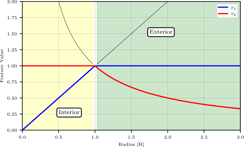
Figure 3: Visualization of $r_{i}$ and $r_{e}$ features.

3.2 Modified Loss Function to Account for high altitude Samples

The loss function for the original PINN-GM is a root mean squared (RMS) error metric:

$$\mathcal{L}_{\text{RMS}}(\mathbf{\theta})=\frac{1}{N}\sum^{N}_{i=0}\sqrt{\left|-\nabla\hat{U}(\bm{x}_{i}|\mathbf{\theta})-\bm{a}_{i}\right|^{2}}$$ (9)

This loss function is common in machine learning regression problems, as it minimizes the most flagrant residuals between the true and predicted values. For the PINN-GM, this means minimizing the difference between the differentiated network potential, $\nabla\hat{U}(\bm{x}_{i}|\theta)$, and the true acceleration, $\bm{a}_{i}$, to satisfy the differential equation $-\nabla U=\bm{a}$. Despite its popularity, this loss function comes with an unexpected disadvantage when applied to the gravity modeling problem.

Gravitational accelerations produced closer to a celestial body have much larger magnitudes than the accelerations produced at high altitudes. As a consequence, even small relative errors in low-altitude predictions will appear disproportionately large compared to any high altitude errors. This means gravity models trained with the RMS cost function will always prioritize accurate modeling in low-altitude regimes at the expense of high-altitude regimes, even if the high-altitude predictions are more erroneous in a relative sense.

To combat this challenge, PINN-GM-III augments the original RMS loss function with an additional mean percent error term through:

$$\mathcal{L}_{\text{RMS+\%}}(\mathbf{\theta})=\frac{1}{N}\sum^{N}_{i=0}\left(\sqrt{\left|-\nabla\hat{U}(\bm{x}_{i}|\mathbf{\theta})-\bm{a}_{i}\right|^{2}}+\frac{|-\nabla\hat{U}(\bm{x}_{i}|\mathbf{\theta})-\bm{a}_{i}|}{|\bm{a}_{i}|}\right)$$ (10)

By incorporating a percent error loss, the PINN-GM-III is no longer exclusively biased by the absolute magnitudes of the acceleration vectors, but instead also minimizes relative errors. This design change ensures that all samples, regardless of altitude, are contributing meaningfully to the loss function and are prioritized by the network during training.

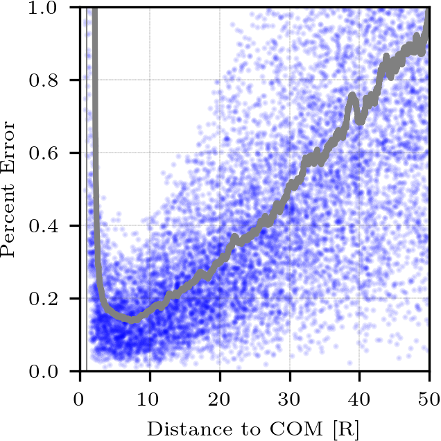
(a) $\mathcal{L}_{\text{RMS}}$ Loss Function

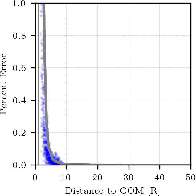
(b) $\mathcal{L}_{\text{RMS}+\%}$ Loss Function

Figure 4: Different loss function change network performance at high and low altitudes. Blue points are the individual errors of the test data, and the gray line is the average test error within a sliding window of 250 points.

To illustrate the effect of the new loss function on model performance, a test is proposed which trains two PINN-GMs on 1,000 position / acceleration training data pairs distributed from 0-50 radii above the asteroid Eros’s surface. One PINN-GM is trained using the original RMS loss function and the other is trained on with the augmented loss function. Once trained, each network is evaluated on a set of 10,000 randomly distributed test points from 0-50R, and the percent error of their acceleration vectors are reported as a function of altitude in Figure 4. Figure 4(a) confirms that the networks trained with the RMS loss function disproportionally favor low-altitude field points ($<5$R) at the expense high-altitude field points ($>$5R) despite being trained across the entire 0-50R domain. In contrast, the PINN-GM model trained with the augmented loss function (Figure 4(b)) prioritizes accurate modeling across all altitudes.

3.3 Improve Numerics by Learning a Proxy to the Potential

All gravitational potentials decay at high altitudes according to an inverse power law of $1/r$. This decay poses numerical challenges when operating PINN-GM models at high altitude. Consider that the largest gravitational potential represented by the network is non-dimensionalized to one from Equations (5) and (6). For field points at a sufficiently high altitude, the neural network will need to compute potentials which decay to values to less than or equal to machine precision (i.e. $U(r\rightarrow r_{\text{crit}})\leq\epsilon_{\text{machine}}$). Representing these vastly different numerical scales with the same neural network is undesirable and can lead to numerical instability during training and inference, and unnecessarily capping the maximum altitude for which the model is viable.

PINN-GM-III addresses this phenomenon by learning a more numerically favorable proxy to the potential that can be later transformed into the correct order of magnitude. Explicitly, PINN-GM-III learns a proxy to the potential referred to as $U_{\text{NN}}$ defined as

$$U_{\text{NN}}=U*n(r)\mathchar 24635\relax\;\quad n(r)=\begin{cases}1\quad r<R\\ r\quad r>R\\ \end{cases}$$ (11)

where $U$ is the true potential and $n(r)$ is a scaling function. By introducing this scaling function, the direct output of the neural network, $U_{\text{NN}}$, always remains bounded and centered about a non-dimensionalized value of $\mu$. This centering lowers the risk of numerical error and avoids prematurely capping the accuracy of the model at high altitudes. After the network produces its value of the proxy potential, it is then explicitly transformed into the true potential distribution / correct order of magnitude by dividing by the prescribed scaling function through

$$\hat{U}_{\text{NN}}=\frac{U_{\text{NN}}}{n(r)}$$ (12)

The effect of this change is illustrated in Figure 5 which shows the true potential and the proxy potential for the asteroid Eros between 0-10R. Rather than learning a distribution that continuously decays at high altitudes, the network instead learns a distribution centered and bounded about the true, non-dimensionalized value of $\mu$. As the altitude increases, the point mass approximation becomes increasingly representative of the true system, allowing the distribution to converge on the true value of $\mu$.

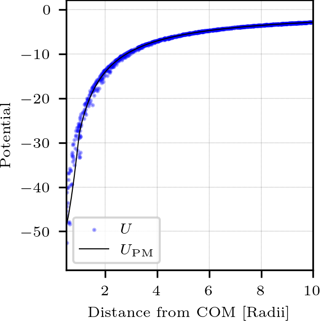
(a) True potential $U$

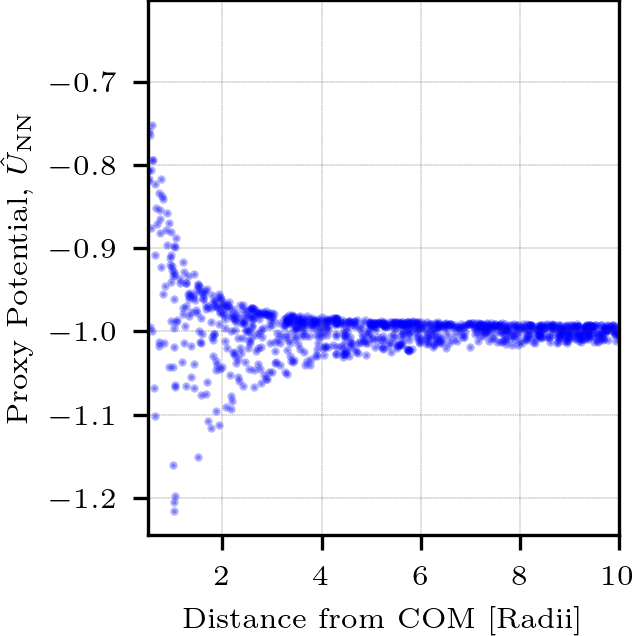
(b) Proxy potential, $U_{\text{NN}}$

Figure 5: The true potential $U$ (left) quickly decays to numerically unfavorable values whereas versus the proxy potential $U_{\text{NN}}$ (right) remains centered and bounded about the non-dimensionalized value of $\mu$.

3.4 Enforcing Boundary Conditions through Model Design to Avoid Extrapolation Error

While PINNs are most commonly designed to satisfy physics through their cost function, there are also other ways to enforce compliance through the design of the machine learning model itself. Reference 40 shows how machine learning models can be designed to seamlessly blend between a network solution and known analytic boundary conditions through the use of Heaviside-like functions.

To achieve a similar effect, PINN-GM-III proposes the following design modification to enforce relevant boundary constraints:

$$\hat{U}(r) =w_{\text{NN}}(r)\hat{U}_{\text{NN}}(r)+w_{\text{BC}}(r)U_{\text{BC}}(r)$$ (13)

where $\hat{U}_{\text{NN}}$ is the predicted gravitational potential, $U_{\text{BC}}$ is the potential at the boundary condition, and $w_{\text{NN}}$ and $w_{\text{BC}}$ are the altitude dependent weights for each defined as:

$$w_{\text{BC}}(r,k,r_{\text{ref}}) =H(r,k,r_{\text{ref}})$$ (14)

$$w_{\text{NN}}(r,k,r_{\text{ref}}) =1-H(r,k,r_{\text{ref}})$$ (15)

where $H(r)$ is a Heaviside-inspired function defined as

$$H(r,k,r_{\text{ref}})=\frac{1+\tanh(k(r-r_{\text{ref}}))}{2}$$ (16)

where $r$ is the radius of the field point, $r_{\text{ref}}$ is a reference radius, and $k$ is a smoothing parameter to control for a more continuous or discrete transition. $r_{\text{ref}}$ is typically chosen to be the maximum altitude of the training bounds and the recommended value of $k$ is 2. This heuristic choice balances assurance that the model will quickly transition to the analytic model outside the training data without applying the transition too rapidly that it changes gradient of the potential and introduces error into the acceleration predictions. A visualization of these evolving weights are shown in Figure 6.

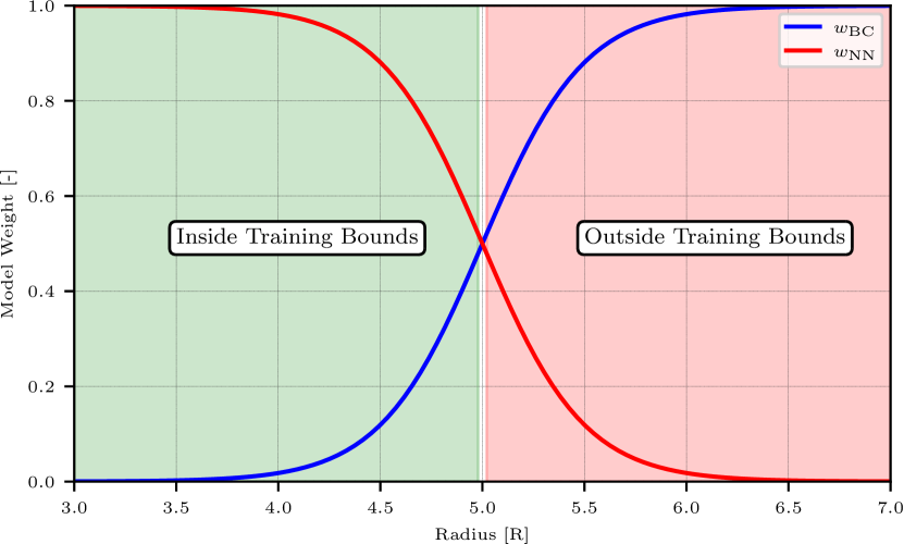
Figure 6: Visualization of the relative weights of the analytic and neural network models as determined by $H(r,k,r_{\text{ref}})$.

Equation (16) enforces that the PINN-GM must smoothly transition into a known boundary condition past the reference altitude $r_{\text{ref}}$. In this way, the machine learning model can leverage the modeling flexibility of the neural network to represent complex regions of the gravity field near the body for which the boundary condition is irrelevant, but then smoothly decrease the network’s responsibility in the limit as the model approaches the boundary.

For the gravity modeling problem, there exists multiple ways in which this design choice can manifest. In the limit of $r\rightarrow\infty$, the potential decays to zero as discussed in Section 3.3. However, setting $U_{\text{BC}}=0$ and $r_{\text{ref}}=\infty$ in Equation (13) is not practical as it demands the neural network must learn a model of the potential for the entire domain $r\in[0,\infty)$. A more useful choice is to leverage insights from the spherical harmonic gravity model and recognize that high frequency components of the gravitational potential decay to zero more quickly than the point mass contribution at high altitudes. i.e.

$$U_{\text{BC}}(r)=U_{\text{LF}}=\frac{\mu}{r}+\cancelto{0}{\sum_{l=0}^{n}\sum_{m=0}^{l}\frac{\mu}{r}\left(\frac{R}{r}\right)^{l}(\ldots)}$$ (17)

as $r\rightarrow\infty$.

This observation implies that $U_{\text{BC}}(r)$ can be set to $\frac{\mu}{r}$ assuming $r\gg R$. As such, the PINN-GM-III sets $U_{\text{BC}}=\frac{\mu}{r}+f(r)$ in Equation (13), where $f(r)$ are any higher order terms in the spherical harmonic gravity model that the user knows a priori and wishes to leave as part of the boundary condition.

3.5 Leveraging Preexisting Gravity Information into PINN-GM Solution

In addition to enforcing the boundary condition through the model design, another design choice enabled by the PINN-GM-III is the ability to fuse prior gravity models with the neural network solution. For example, most large celestial bodies exhibit planetary oblateness which is succinctly captured with the $C_{2,0}$ spherical harmonic coefficient as discussed in Section 2. Rather than requiring the network to relearn this prominent and easily observable perturbation, this information can be directly combined with the network model. In this way, the PINN-GM-III can predict accelerations by leveraging a low-fidelity, first-order analytic model with a network responsible for capturing high-order perturbations through:

$$\hat{U}(r)=w_{\text{NN}}\big{(}U_{\text{LF}}(r)+\hat{U}_{\text{NN}}(r)\big{)}+w_{\text{BC}}\big{(}U_{\text{LF}}(r)\big{)}$$ (18)

where $U_{\text{LF}}$ refers to the known, low-fidelity analytic model such as $U_{\text{LF}}=\frac{\mu}{r}+U_{J_{2}}$.

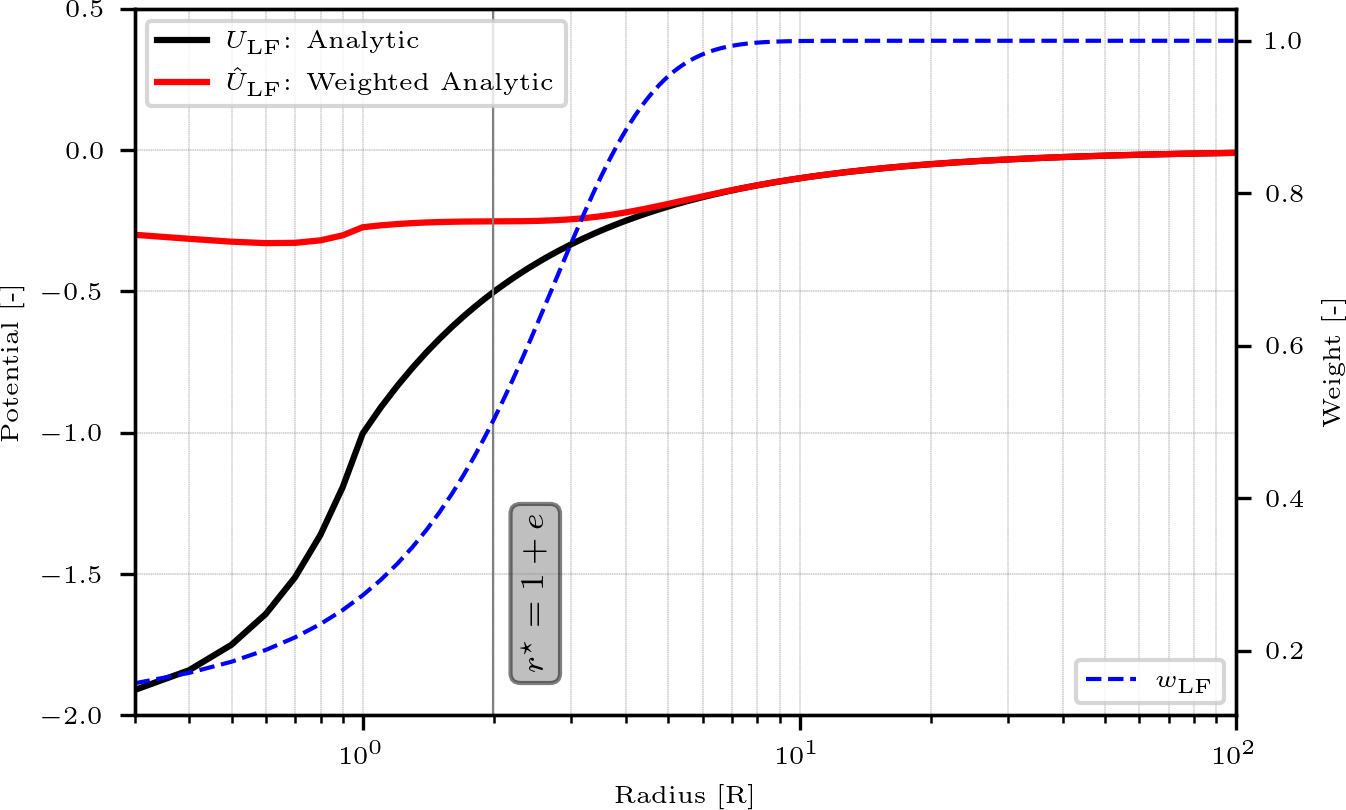
Figure 7: The low-fidelity potential $U_{\text{LF}}$ is downweighted at low-altitudes to become $\hat{U}_{\text{LF}}$ before getting fusing with $\hat{U}_{\text{NN}}$.

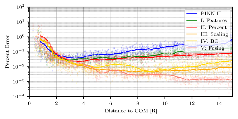
(a) Error inside the training bounds

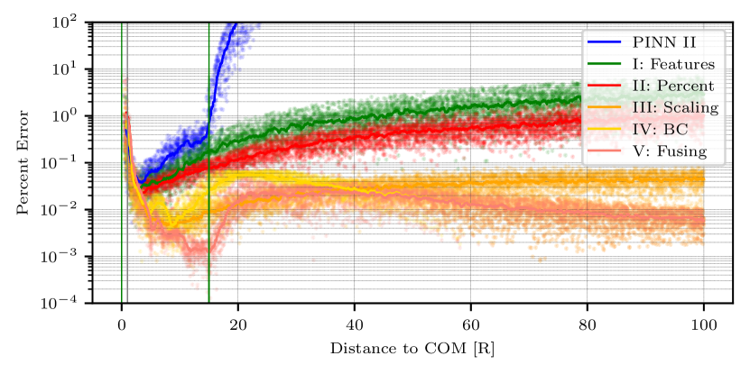
(b) Error outside the training bounds

Figure 8: Acceleration percent error as a function of altitude after sequentially applying each of the proposed PINN III modifications.

In the case of small-body gravity modeling, where the geometries may vastly differ from a point mass or low-fidelity spherical harmonic approximation, the incorporation of past analytic models should be performed carefully, as the analytic models are often only valid at high-altitudes. To ensure that these analytic models are only used where appropriate, the hyperbolic tangent fusing function, $H(x,r,k)$, is reused. Specifically, for small bodies, PINN-GM-III uses

$$\hat{U}_{\text{LF}}(r)=w_{\text{LF}}U_{\text{LF}}(r)$$ (19)

as the low fidelity analytic contribution to the model where $w_{\text{LF}}=H(r,R^{*},k^{*})$, $R^{*}=1+e$, and $k=0.5$, where $e$ is the eccentricity of the body computed via $e=\sqrt{1-b^{2}/a^{2}}$. This ensures that at high altitude, where the analytic approximation is most accurate, it fully contributes to the final learned solution, but at lower altitudes, the analytic contribution has a reduced weight to the final solution. A visualization of this weighted low-fidelity analytic model is shown in Figure 7, and shows how the low fidelity point mass approximation is downweighted at low altitudes, but contributing fully at higher altitudes.

3.6 Analysis of PINN-GM-III Modifications on Model Accuracy

To visualize how the proposed changes affect model accuracy, five PINN-GM are trained, sequentially adding each of the modification listed above. Each of the PINN-GM are trained with the same 5,000 point training data set uniformly distributed between the surface of the asteroid Eros to an altitude of 15$R$. The corresponding acceleration error is reported within the training distribution in Figure 8(a), and outside the training distribution in Figure 8(b).

Figure 8(b) highlights how the former PINN-GM-II is unable to accurately model high altitude samples, and quickly diverges when tested outside of the bounds of the training data. Applying the new radial features (I) reduces this extrapolation error considerably; however the error at high altitudes still monotonically increases and peaks, on average, at 3% at 100R. Incorporating the percent error into the loss function (II) further reduces these errors—from 3% to approximately 1% — by decreasing the sensitivity to the low-altitude field points. The proxy potential feature (III) drops the error down nearly two orders-of-magnitude — from 1% to 0.03% — albeit the error plateaus after approximately 40R. When the boundary condition is added (IV), transitioning the neural network solution into the analytic point mass approximation, and the error in the limit reduces to 0.007%. Incorporating the boundary condition does come with a slight performance penalty at the transition point near 15R, as the transition function introduces an unwanted change in the gradient of the potential. Finally, superimposing the analytic potential with the neural network potential further reduces the error within the bounds of the training data, and returns to the minimum error of 0.007% at the high altitude limit. Note that there exists a numerical floor in the percent error at approximately 0.001% where the differences between model prediction and the ground truth are functionally identical.

4 Case Study: Heterogeneous Density Asteroid

To further illustrate the modeling capabilities of the PINN-GM-III, a case study is performed in which the PINN-GM-III is trained to represent the gravity field of a heterogeneous density asteroid modeled after 433-Eros. Heterogeneous asteroids provide an especially challenging scenario for gravity models, as their internal density distributions are not directly observable. Often assumptions of constant density are made, particularly in the case of the polyhedral model, but recent findings suggest this assumption is not always valid scheeresHeterogeneousMassDistribution2020 . Some asteroids may contain over and under dense regions within their interior, or may have been formed by two asteroids merging together, each with different densities. To capture these inhomogeneities, dynamicists currently make informed assumptions about these distributions based on the asteroid’s gravity field and shape and compare the measured spherical harmonic coefficients against those that would be generated by their assumed profile takahashiMorphologyDrivenDensity2014 . At best, this process leaves researchers with heuristic assessments of the body’s density profile which can be used in heterogeneous forms of the polyhedral model. More often, however, it remains common practice to simply proceed with a constant density assumption. This section explores the ramifications of this choice and highlights how the PINN-GM can bypass many of the consequences of this practice.

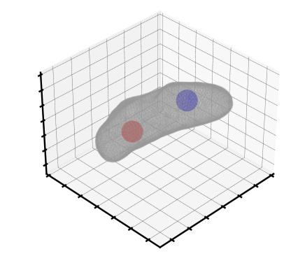
Figure 9: Asteroid with imposed mass heterogeneities

4.1 Problem Setup

For this experiment, two small mass heterogeneities are introduced to the asteroid 433-Eros. In one hemisphere, a mass element is added to the interior of the body, and in the other hemisphere, a mass element is removed. Each mass element contains 10% of the total mass of the asteroid, and they are symmetrically displaced along the x-axis by 0.5R (see Figure 9). The gravitational contributions of these mass elements are superimposed onto the gravity field of a constant density polyhedral model. This emulates the gravity field of a single body formed by two merged asteroids of different characteristic densities. The choice to make each mass element $\pm 10$% of the total mass is motivated based on literature with similar candidate density distributions kanamaruEstimationInteriorDensity2019 .

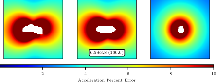
Figure 10: Constant density polyhedral error expressed as $e_{a_{\mu}}\pm e_{a_{\sigma}}(e_{a_{\text{Max}}}$).

These small mass heterogeneities can have large consequences on the corresponding gravity field of the asteroid. If dynamicists continue to model the body under the assumption of constant density, spacecraft trajectories will quickly deviate from their reference and may risk their safety over longer timespans or during mission critical operations. This error is best illustrated through Figure 10 which shows the relative acceleration error of a constant density polyhedral model on the XY, XZ, and YZ planes out to 3$R$ and reports the average, standard deviation, and maximum errors. At higher altitudes, the constant density assumption induces relatively small errors, averaging approximately 4% error. However, at lower altitudes, the constant density assumption grows increasingly unreliable. Within 2 radii of the center of mass, the average error surpasses 10% and rises to errors as large as 160% near the surface.

These errors show why alternative gravity models are needed. Despite the constant density polyhedral model offering the most compelling framework to capture the effect of irregular body geometries on a gravity field, it is not sufficient for modeling density heterogeneities. Moreover, the shape model required over 200,700 facets to represent the full geometry to high levels of fidelity. Even if the polyhedral model was better suited to capture heterogeneities, it would still remain a costly option due to its large memory and computational footprint. The PINN-GM provides a candidate solution to this problem, with the ability to regress a field in a manner agnostic of the body geometry and density profile using considerably fewer parameters.

To illustrate this, a PINN-GM-II and a PINN-GM-III are trained from a set of position and acceleration data to regress a model of this complex field. This is accomplished using a network architecture of six hidden layers with 32 nodes per layer (approximately 6,500 parameters), and regressed under ideal data conditions. The training dataset includes 90,000 data points distributed uniformly between 0-10R, as well as 200,000 samples distributed directly on the surface of the asteroid. These optimistic data conditions are used to establish an approximate upper bound on performance for the PINN-GMs at this parametric capacity. Suboptimal and sparse data conditions are investigated later in Section 5.

4.2 Metrics

The performance of the PINN-GM-II and III are compared to that of the constant density polyhedral model through a comprehensive suite of metrics outlined in the following subsection. These metrics explore the performance of the model within and beyond the bounds of the training data, as well as characterize additional properties of interest such as execution time and accumulated trajectory error.

Planes Metric

The first metric assesses the mean acceleration percent error of the learned gravity model along the three cartesian planes (XY, XZ, YZ) extended between [-5R, 5R] where R is the radius of the asteroid. The field is evaluated on a 200x200 grid of points along each plane, and the average percent error is computed as

$$P=\frac{1}{N}\sum_{i=1}^{N}\frac{|\bm{a}_{\text{true}}-\bm{a}_{\text{PINN}}|}{|\bm{a}_{\text{true}}|}\times 100$$ (20)

This metric is intended to provide a high-level measure of model performance across a wide range of operational regimes.

Generalization Metrics

The second, third, and fourth metrics investigate the generalization of the model across a range of altitudes both within and beyond the training bounds. Explicitly, the mean acceleration error is evaluated as a function of altitude, and divided into three testing regimes: interior, exterior, and extrapolation. The interior metric assesses error within the bounding sphere of radius R. The exterior metric investigates the error between R and the maximum altitude of the training dataset at 10R. Finally, the extrapolation metric measures the error for altitudes beyond the training dataset ranging from 10R to 100R. Note that for every unit of radius, 500 samples are distributed uniformly in altitude to produce the test set.

Surface Metric

The fifth metric evaluates the mean acceleration error across all facets on the surface of the high-resolution shape model. For the heterogeneous density model of 433-Eros used in this experiment, 200,700 facets are used to compute the mean. This metric is used to characterize model performance at the most complex and dynamically significant region of the field.

Trajectory Metrics

The sixth metric evaluates the accumulated trajectory propagation error over one day of simulation time for a spacecraft in a low altitude polar orbit about a rotating asteroid:

$$\mathcal{S}=\int_{t=0}^{T}\Delta\bm{X}_{i}(t)\text{d}t\approx\sum_{j=0}^{N}|\Delta\bm{X}_{i}(t_{j})|$$ (21)

where the orbit is defined used is defined as $\{a,e,i,\omega,\Omega,M\}=\{32\text{ km},0.1,90^{\circ},0^{\circ},0^{\circ},0^{\circ}\}$, and the asteroid is rotating at $\omega_{0}=0.00073$ degrees per second along the z-axis. The accumulated position error serves as a practitioner’s metric to determine how much error trajectory designers can expect when using these models. Finally, the seventh metric evaluates the total time needed to propagate the orbit.

4.3 PINN-GM-III Performance

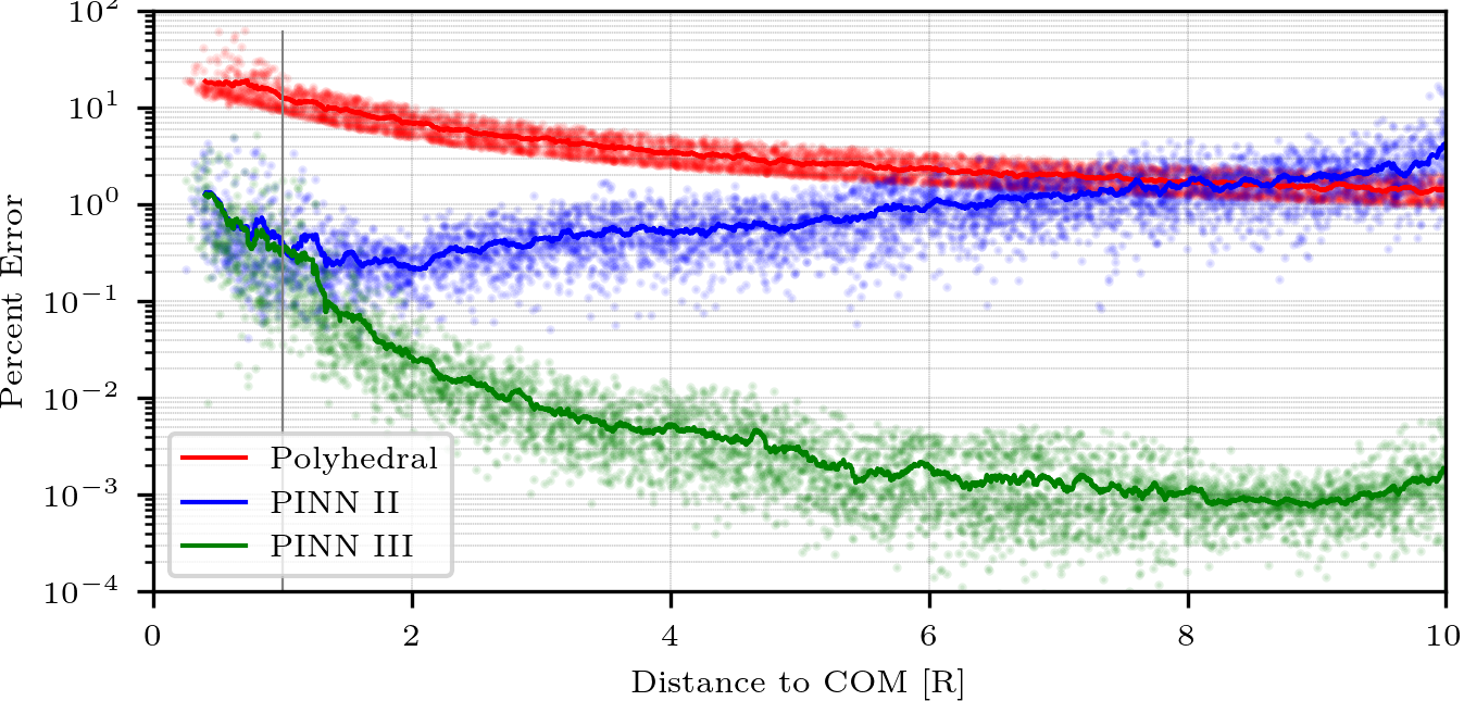
Generalization

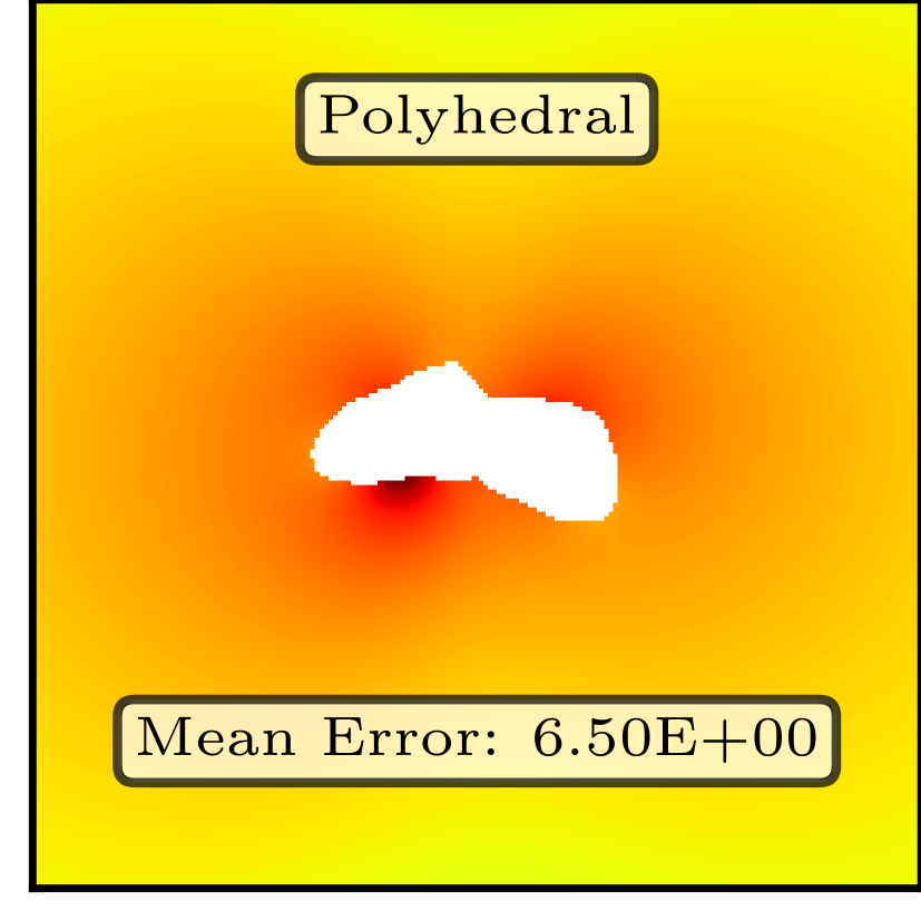
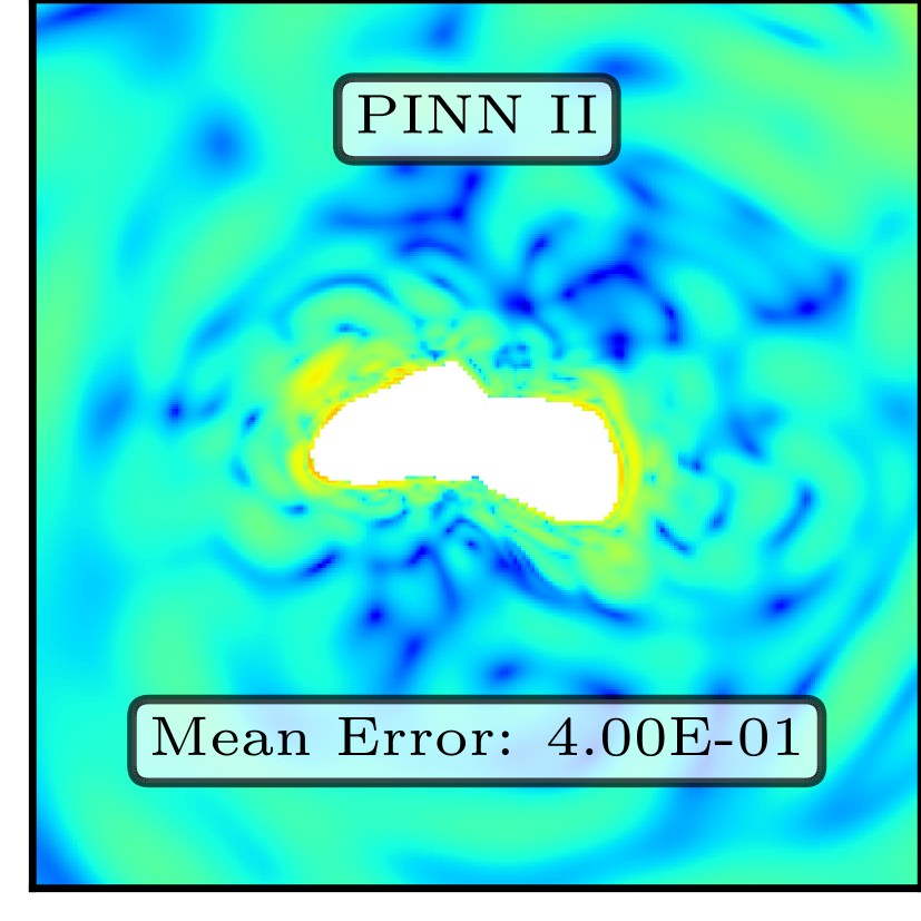
Planes

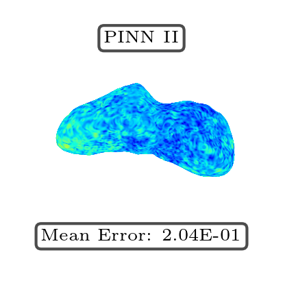
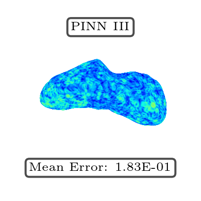
Surface

Trajectory

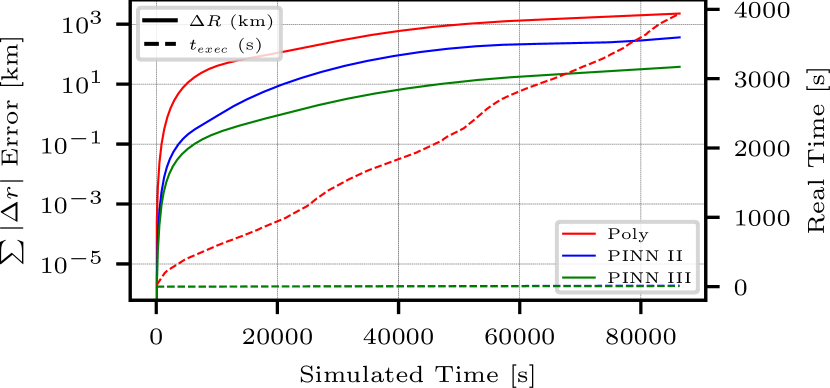
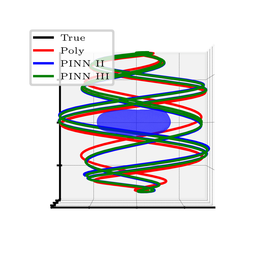
Figure 11: All proposed metrics evaluated for the constant density polyhedral model, the PINN-GM-II, and the PINN-GM-III.

These seven metrics are used to evaluate the performance of three gravity models: the high-resolution constant density polyhedral gravity model, a PINN-GM-II, and a PINN-GM-III. The polyhedral model contains 200,700 facets, and the PINN-GM models contain six hidden layers of 32 nodes each, corresponding to a model size of approximately 6,500 parameters. The polyhedral model is precomputed agnostic to the training data, and PINNs are trained using the distribution described above and using the default hyperparameters determined in Appendix B. The corresponding results are shown in Figure 11.

Beginning with the generalization experiment, the top of Figure 11 demonstrates that the constant density polyhedral model produces the highest error within the test domain. The PINN-GM-II performs considerably better near the surface, but accuracy deteriorates at high altitudes as a result of the faulty RMS loss function. In contrast, the PINN-GM-III produces errors between one and three orders of magnitude lower than the constant density polyhedral model, offering superior performance at both low and high altitudes. The planes and surface metrics further this narrative as shown in the middle rows of Figure 11. Here the polyhedral gravity model produced an average acceleration error of 6.5% on the planes metric, and the PINN-III reduces this by nearly two orders of magnitude. On the surface, a similar effect is shown with the polyhedral model averaging 23% error, and the PINN-III reducing this to 0.18%.

The bottom of row of Figure 11 shows the trajectory propagation experiment and demonstrates the PINN-IIIs considerably faster propagation speed and lower propagation error. Placing the spacecraft in the polar orbit about a rotating asteroid for one simulated day of flight requires over one hour of compute time with the polyhedral model, and accumulates over 2000 kilometers of error. In contrast, the PINN-III requires only 8 seconds to propagate and accumulates 38 km of error. Note that the more intuitive instantaneous position error at the end of the orbit is 4.6km for the polyhedral model and 0.1km for PINN-III. The accumulated error is chosen for plotting as it provides a monotonically increasing measure of trajectory propagation error.

Taken together, the PINN-III provides consistently superior performance to both its analytic and numerical predecessors, offering significant improvements in modeling accuracies across a wide range of metrics while using a considerably smaller parametric footprint. Notably, the PINN-GM performance can improve with higher capacity models and additional training data. While these performance measures are encouraging, they are only representative of ideal modeling conditions for which perfect position and acceleration data exists and can be used for training. The next section explores what happens under less ideal data conditions and extends the study to investigate the PINN-IIIs performance against additional analytic and numerical models.

5 Comparative Study

In this section, a comparative study is performed to evaluate the accuracy of the PINN-GM-III against other popular gravity models. Explicitly, a point mass (PM), spherical harmonic (SH), mascon, polyhedral, extreme learning machine (ELM), traditional neural network (TNN), PINN-GM-I, and PINN-GM-II model are each fit on various data conditions and then evaluated using the aforementioned metrics.

Each model is fit four times, permuting the data quantity and the parametric capacity of each model. Explicitly, each model is fit once with 500 data points, and once with 50,000 data points to illustrate model sensitivity to data quantity. In both cases, the data is uniformly distributed between 0-10R using the same heterogeneous density asteroid from Section 4. In addition, each model is tested at “small” and “large” parametric capacity. These labels correspond to the total number of parameters, $p$, contained within the model (e.g. Stokes coefficients for a spherical harmonic model, facets and vertices in a shape model, or total weights and biases in a neural network). Each small model contains approximately 250 parameters, whereas the large models have approximately 30,000 parameters. Together, these varying data and parametric conditions provide insight into which models are capable of maintaining competitive performance under data-sparse and low-memory conditions. Note that each model has slightly different regression procedures and model size calculations which are detailed in Appendix D.

	Planes	Generalization			Surface	Trajectory		Auxillary
	Error[%]	Extrapol. Error[%]	Exterior Error[%]	Interior Error[%]	Error[%]	Position Error[km]	Propagation Time[s]	Params	Regression Time[s]
PM	52.8	53.4	53.5	44.6	69.6	1.2e5	0.0	1.0	0.7
SH	D	0.3	5.0	D	D	4.4e3	0.1	240.0	4.3
Poly.	6.2	0.3	3.3	15.9	23.3	1.9e3	1.6	204.0	NA
Mascons	3.1	2.7	2.8	4.4	41.4	8.2e3	0.6	220.0	4.9
ELM	D	D	D	D	D	2.0e9	6.8	280.0	2.2
TNN	D	D	D	D	D	5.8e5	149.9	257.0	726.1
PINN I	14.4	D	37.6	8.3	31.1	2.5e4	114.5	256.0	800.2
PINN II	0.6	D	0.6	1.7	12.7	273.1	22.4	200.0	971.6
PINN III	0.4	0.1	0.1	2.6	17.7	56.5	22.4	227.0	862.0
N = 50000 Samples;  Model Size = ’Small’
PM	NA	NA	NA	NA	NA	NA	NA	NA	NA
SH	D	0.3	5.0	D	D	4.4e3	0.4	3.1e4	8.2e3
Poly.	6.5	0.4	3.5	16.5	23.3	2.3e3	132.3	3.0e4	NA
Mascons	0.0	0.0	0.0	0.1	32.8	2.7e3	6.2	3.0e4	471.7
ELM	D	D	D	D	D	5.1e7	33.5	3.6e4	262.3
TNN	D	D	D	D	D	6.4e5	62.2	2.9e4	973.3
PINN I	10.4	D	8.3	4.2	8.8	1.1e4	35.1	2.9e4	995.3
PINN II	0.0	D	0.0	0.1	2.8	9.6	15.3	3.0e4	1.7e3
PINN III	0.0	1.1	0.0	0.1	3.3	8.4	18.5	3.0e4	1.6e3
N = 50000 Samples;  Model Size = ’Large’
PM	49.9	50.3	50.5	43.2	69.6	1.2e5	0.0	1.0	0.6
SH	25.7	0.3	5.0	D	D	4.4e3	0.1	240.0	2.7
Poly.	6.2	0.3	3.3	15.9	23.3	1.9e3	1.6	204.0	NA
Mascons	2.7	1.8	1.9	12.3	D	6.4e3	0.5	220.0	2.1
ELM	74.2	D	D	98.0	99.3	6.6e4	0.9	280.0	0.0
TNN	D	D	D	D	D	4.5e5	75.7	257.0	154.9
PINN I	38.3	D	75.2	23.8	42.0	4.7e4	84.0	256.0	129.0
PINN II	2.5	D	2.9	8.2	30.4	3.0e3	23.9	200.0	133.2
PINN III	1.5	0.3	0.4	8.6	31.3	1.1e3	14.0	227.0	128.7
N = 500 Samples;  Model Size = ’Small’
PM	NA	NA	NA	NA	NA	NA	NA	NA	NA
SH	D	0.3	5.0	D	D	4.4e3	0.3	3.1e4	97.7
Poly.	6.5	0.4	3.5	16.5	23.3	2.3e3	132.3	3.0e4	NA
Mascons	0.7	0.0	0.0	10.9	D	2.7e3	6.9	3.0e4	138.6
ELM	75.8	D	D	97.3	99.1	6.5e4	1.1	3.6e4	4.3
TNN	D	D	D	D	D	7.8e5	162.7	2.9e4	145.2
PINN I	49.3	D	D	37.8	37.7	5.5e4	51.0	2.9e4	150.3
PINN II	0.7	D	0.2	5.5	25.9	196.5	15.4	3.0e4	177.6
PINN III	1.6	0.4	0.2	17.3	51.0	406.6	20.8	3.0e4	173.9
N = 500 Samples;  Model Size = ’Large’

Table 2: Gravity metrics evaluated after regression on noiseless training data.

Regression with Perfect Data

The experiment begins with perfect position and acceleration training data with no error. The metrics associated with each regressed model are provided in Table 2. Across both data-rich and data-sparse conditions, and using large and small parametric models, the PINN-GM-III’s performance across the seven metrics remains competitive, if not superior, to all past analytic and numerical models. Explicitly, under data-rich conditions where $N=50,000$, the PINN-III is typically the best performing model in the both the large and small parametric configurations. As demonstrated by the first two sub-tables in Table 2, the PINN-III is only outperformed by an analytic model in the total trajectory propagation time; however, the lower propagation time of these models comes at the cost of higher total accumulated trajectory error. Across the percent error metrics, the PINN-III is usurped by the PINN-II only at the surface and by a small margin. Moreover there is one occasion in which the mascon model does have a lower error in the regions outside the training data; however this is to be expected given that the PINN-III transitions into the low fidelity point mass approximation beyond the bounds of the training data as described in Section 3.4.

In the data sparse conditions where only $N=500$ data exist between 0-10R, all models’ performance deteriorates as expected; however, the PINN-III remains the most robust option. As shown by the bottom two sub-tables in Table 2, the PINN-III is the only model besides the polyhedral solution that never diverges — where diverging is defined as errors $>$100% and denoted by “D” in the table. While the PINN-II has a slightly lower error near the surface, and the mascon model has lower error at high altitudes, both of these models diverge in other regions whereas the PINN-III does not. Moreover, the PINN-III remains relatively agnostic to overfitting even when the parametric capacity is increased to $p\approx 30,000$.

Notably, despite the PINN-III performance being the most accurate option in data-rich conditions, and the most robust in data-sparse conditions, it should be noted that these gains come at the expense of longer regression times. All results generated in Table 2 are trained on a 2 core processor with access to an A100 GPU. In this configuration, the PINN-GMs consistently take the longest to train, ranging between 120 seconds for the small models with the small data sets to over 30 minutes for the largest models with the most data.

While regression times presented for the analytic models are consistently faster, it should be noted this may not always be the case. All of the analytic models tested in this experiment are regressed sequentially in small batches to avoid the large amounts of memory and compute time that would be necessary to perform a full least-squares matrix inversion. This choice sacrifices some performance in the analytic models, but these models would otherwise be infeasible to regress given the available compute resources. Conversely, the PINN-GMs training times could be significantly reduced if larger mini-batch sizes are used. While the A100 GPUs used have sufficient memory to accommodate these larger batch sizes, it does come at the expense of slightly less accurate models as shown in ablation studies of Appendix B. The results presented in Table 2 are an attempt to balance these factors, but it should be stressed that users can effectively trade regression time with accuracy for both the analytic and numerical models.

	Planes	Generalization			Surface	Trajectory		Auxillary
	Error[%]	Extrapol. Error[%]	Exterior Error[%]	Interior Error[%]	Error[%]	Position Error[km]	Propagation Time[s]	Params	Regression Time[s]
PM	52.8	53.3	53.4	44.6	69.6	1.2e5	0.0	1.0	0.7
SH	D	0.3	5.0	D	D	4.4e3	0.1	240.0	5.5
Poly.	NA	NA	NA	NA	NA	NA	NA	NA	NA
Mascons	3.3	3.0	3.0	4.6	41.6	9.0e3	0.5	220.0	5.6
ELM	D	D	D	D	D	1.9e9	7.8	280.0	2.5
TNN	D	D	D	D	D	7.6e5	91.6	257.0	232.5
PINN I	16.3	D	38.4	10.1	33.3	4.8e3	132.9	256.0	683.3
PINN II	2.1	D	2.9	3.2	15.1	1.4e3	29.7	200.0	141.4
PINN III	3.9	0.3	2.0	8.3	35.0	3.0e3	15.8	227.0	37.8
N = 50000 Samples;  Model Size = ’Small’
PM	NA	NA	NA	NA	NA	NA	NA	NA	NA
SH	D	0.3	5.0	D	D	4.4e3	0.4	3.1e4	8.0e3
Poly.	NA	NA	NA	NA	NA	NA	NA	NA	NA
Mascons	1.3	0.1	0.2	9.3	D	2.4e3	6.2	3.0e4	471.9
ELM	D	D	D	D	D	4.7e7	22.4	3.6e4	255.7
TNN	D	D	D	D	D	8.0e5	29.0	2.9e4	59.8
PINN I	13.8	D	29.9	6.1	17.0	1.3e4	28.8	2.9e4	77.8
PINN II	1.4	D	2.2	2.7	8.9	799.9	15.3	3.0e4	81.3
PINN III	3.4	0.3	2.0	3.7	12.7	6.3e3	20.2	3.0e4	66.9
N = 50000 Samples;  Model Size = ’Large’
PM	50.1	50.6	50.7	43.3	69.6	1.2e5	0.0	1.0	0.7
SH	25.1	0.3	5.0	D	D	4.4e3	0.1	240.0	1.5
Poly.	NA	NA	NA	NA	NA	NA	NA	NA	NA
Mascons	34.1	28.4	28.7	98.4	D	5.6e4	0.3	220.0	2.5
ELM	75.6	D	D	97.9	99.3	6.6e4	0.7	280.0	0.0
TNN	D	D	D	D	D	6.4e5	19.8	257.0	27.2
PINN I	32.8	D	70.3	19.4	36.6	3.6e4	86.0	256.0	127.0
PINN II	5.8	D	6.6	12.0	31.9	2.5e3	22.3	200.0	18.0
PINN III	10.7	0.3	3.4	58.0	82.4	2.2e4	14.6	227.0	12.9
N = 500 Samples;  Model Size = ’Small’
PM	NA	NA	NA	NA	NA	NA	NA	NA	NA
SH	D	0.3	5.0	D	D	4.4e3	0.3	3.1e4	91.9
Poly.	NA	NA	NA	NA	NA	NA	NA	NA	NA
Mascons	D	0.6	D	D	D	NA	NA	3.0e4	157.5
ELM	77.6	D	D	97.2	99.0	6.5e4	1.0	3.6e4	4.4
TNN	D	D	D	D	D	5.0e5	20.8	2.9e4	18.0
PINN I	30.5	D	48.8	17.4	33.2	3.2e4	40.8	2.9e4	17.9
PINN II	5.9	D	5.0	13.4	32.3	7.1e3	16.0	3.0e4	22.4
PINN III	6.1	0.4	3.0	27.1	49.5	6.4e3	20.8	3.0e4	19.8
N = 500 Samples;  Model Size = ’Large’

Table 3: Gravity metrics evaluated after regression on noisy (10%) training data.

Regression with Noisy Data

The past experiment demonstrates how the analytic and numerical gravity models perform under the assumption of perfectly measured training data. This experiment explores how the models fare under more challenging conditions where the training data may be noisy. To accomplish this, the same regressions are performed, but every acceleration vector in the training data is perturbed in a random direction by 10% of the original acceleration magnitude. This error is chosen as an exaggerated test case to determine which of these models remain reliable under more stressful data conditions. The polyhedral model is purposefully excluded from this experiment as there is no straightforward way to incorporate the uncertainty of the acceleration vectors onto the resultant shape model. The results of this experiment are provided in Table 3.

Similar conclusions can be drawn from the noisy regression as from the noiseless regression. The PINN-III remains the only robust option that never diverges in both data-rich and data-sparse conditions, as well as for large and small parametric model sizes. Notably, the mascon gravity model offers compelling and occasionally superior performance in the data-rich conditions, but it is prone to diverging at low-altitudes unlike the PINN-III. Importantly, none of the gravity models perform especially well at low-altitudes under data-sparse conditions. While the PINN-III never officially diverges, it can produce errors in excess of 50% inside the bounding sphere, and $>$80% at the surface. While this is better than the other available analytic models, it is advisable to avoid operating in these low-altitude regimes until additional data can be collected, at which performance can reach $<$10% error in the interior regime as shown in the data-rich conditions. At high-altitudes, the PINN-III offers far more satisfying performance with errors less than 3% for all altitudes above $1$R.

In addition to the core performance metrics, the total regression time required to fit the PINN models is far more competitive under the noisy data conditions than under the perfectly measured conditions. This is a result of an early stopping criteria used during training. Explicitly, the training process is prematurely halted if the validation loss does not continue to decrease for a finite set of epochs. This helps prevent overfitting to erroneous data and consequently produces far faster regression times. Under the perfect data conditions, this stopping criteria is never triggered, hence the considerably longer training times.

6 Conclusions

Scientific machine learning and physics informed neural networks (PINNs) offer a new and compelling way to solve the gravity field modeling problem. Rather than using prescriptive analytic gravity models which come with various limitations and pitfalls, PINNs can learn convenient representations of the gravitational potential while maintaining desirable physics properties and small model sizes. While past generations of the PINN-GM have offered early glimpses into the potential advantages of this class of machine learning gravity model, there remained multiple challenges left to be addressed and further opportunities for development. This paper introduces the third generation PINN gravity model, PINN-GM-III, which is specifically designed to overcome these past challenges.

Explicitly, past PINN-GM generations struggle to incorporate high altitude data into their regression, inadvertently prioritizing low-altitude samples as a result of a biased cost function. These former models also suffer from numerical instability at high altitudes, are prone to extrapolation error, and lack a way to incorporate prior models into their regression. The PINN-GM-III proposes key design changes such as using a more robust loss function, learning proxy potentials, incorporating known boundary conditions, and leveraging multi-fidelity models to alleviate these and other challenges.

Together, these design modifications produce more accurate and robust machine learning gravity models than past generations. When modeling heterogeneous density asteroids, the PINN-GM-III consistently achieves competitive, if not superior, performance over past generations and competing analytic models on a variety of metrics. At best, the PINN-GM-III demonstrates orders of magnitude improvements in accuracy over constant density polyhedral models, at a fraction of the model size, granting faster propagation times with lower accumulated error. Moreover, these models maintain competitive modeling accuracy at both large and small model sizes, and under both data-rich and data-sparse conditions. Future work will continue to investigate design modifications that can improve model performance, particularly returning to large celestial bodies and investigating ways in which the high-frequency components can be learned and represented more efficiently given sparse data.

7 Statements and Declarations

On behalf of all authors, the corresponding author states that there is no conflict of interest.

8 Acknowledgements

This work utilized the Alpine high performance computing resource at the University of Colorado Boulder. Alpine is jointly funded by the University of Colorado Boulder, the University of Colorado Anschutz, Colorado State University, and the National Science Foundation (award 2201538).

Appendix A PINN-GM-III Training Details

Like the PINN-GM-II, the PINN-GM-III is built around a core network which shares similarities to a transformer architecture. The network itself is composed of a feed-forward multilayer perception, preceded by an embedding layer. Skip connections are attached between the embedding layer and each of the hidden layers, and the final layer uses linear activation functions to produce the network’s prediction of the proxy potential.

Unlike the PINN-GM-II, all of the experiments tested in this paper do not make use of the multi-constraint loss function. Specifically, in the PINN-GM-II implementation, the loss function included penalties for $\nabla^{2}U=0$ and $\nabla\times\nabla U=0$ in addition to $-\nabla U-\bm{a}=0$. While the multi-objective loss function has offered value when training networks on noisy data in the past, it is shown to no longer be necessary in the ablation studies shown in Appendix B. The default hyperparameters used to train PINN-GM-III are listed in Table 4.

Hyperparameter	Value
learning_rate	$2^{-8}$
batch_size	$2^{11}$
num_epochs	$2^{13}$
optimizer	Adam kingmaAdamMethodStochastic2014
activation_function	GELU hendrycksGaussianErrorLinear2020

Hyperparameter	Value
lr_scheduler	plateau
lr_patience	1,500
decay_rate	0.5
min_delta	0.001
min_lr	1e-6

Table 4: Default Set of Hyperparameters for Neural Network Training

Appendix B Ablation Studies

Neural networks can be sensitive to various hyperparameters, so this section aims to characterize the sensitivity of the PINN-GM to a set of core hyperparameters, as well as determine the effect of different network sizes and quantity / quality of training data. Explicitly, network depth, width, batch size, learning rate, epochs, and loss function are varied, as well as the total amount data and its quality. As before, the heterogeneous density asteroid Eros detailed in Section 5 is used to provide training data. 32,768 training data are produced uniformly between 0-3R, and the network performance is evaluated using a mean percent error averaged across 4,096 separate validation samples.

B.1 Network Size

The first test investigates the PINN-GM’s sensitivity to network size, varying both network depth and width. The network depth is varied between ${2,4,6,8}$ hidden layers, and the width is varied between ${8,16,32,64}$ nodes per hidden layer. The remaining hyperparameters are kept fixed at the defaults provided in Table 4. The mean percent error of the models are reported in Figure 12(a) with the corresponding model size, or total trainable parameters, overlaid on the bars.

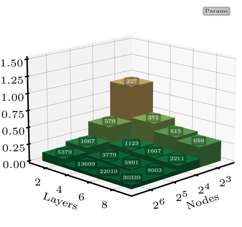
(a) Depth vs width

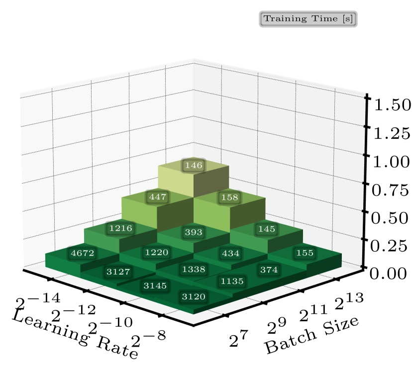
(b) Batch vs Learning Rate

Figure 12: Core Hyperparameters

Figure 12(a) demonstrates that PINN-GM-III performs well across a variety of different network sizes. The smallest networks will perform less well than the largest networks given their considerably smaller parametric capacity, yet despite this, all models remain well below 1.5% error. The smallest model, of 227 trainable parameters, averages at 0.9% error, whereas the largest model with 30,339 parameters achieves 0.3% error. This figure illustrates that optimal models require a minimum of 16 nodes with four hidden layers. Additional layers and nodes will continue to marginally improve performance, but introduces considerable growth model size. Therefore, there comes a point of diminishing return where the model sizes increases as $\mathcal{O}(n^{2})$ despite the average error not experiencing a proprotional reduction. If the compute resources are available, then there is no immediate harm in choosing a higher capacity model, but if optimizing for the best value (smallest model for maximum performance), then it is recommended to use a model of 6 hidden layers and 16 nodes per layer (1667 parameters) or 6 hidden layers and 32 nodes (5891 parameters). In compute constrained environments, such as on-board spacecraft, the smallest model of 227 parameters remains an entirely viable option with its average 0.9% error. The equivalent spherical harmonic model would be a degree and order 15 spherical model which would be inviable for surface or proximity options as discussed in Section 2.

B.2 Batch Size and Learning Rate

After investigating the network size, the next experiment studies the effect of batch size and learning rate on the PINN-GM. Explicitly, the network size is kept fixed at 6 hidden layers and 32 nodes per layer, but the batch size is varied between $\{2^{7},2^{9},2^{11},2^{13}\}$ and the learning rate is varied between $\{2^{-14},2^{-12},2^{-10},2^{-8}\}$. Again the mean percent error of 4,096 samples are evaluated and shown in Figure 12(b), however instead of total model parameters, the total training time is overlaid on the bars.

Figure 12(b) demonstrates that there are a variety of learning rates and batch sizes that remain viable for the PINN-GM. In general, smaller batch sizes do produce more accurate models, albeit this comes with considerably longer training times. Explicitly the training time scales linearly, such that if the batch sizes is decreased by a factor of four, the total training time is approximately four times longer.

For the learning rate, larger is better. This is likely a byproduct of the chosen learning rate scheduler. Typically high learning rates can prevent the networks from converging to their local minimum; however, learning rate schedulers mitigate this risk by continuously decreasing the learning rate such the solution can settle into its local minimum. For these experiments, the learning rate is decreased by a factor of 0.5 every 1,500 epochs that the validation loss does not improve. Given this learning rate scheduler configuration, a learning rate of at least $2^{-8}$ is recommended for most applications.

B.3 Data Quantity and Epochs

From these two initial experiments, a final set of optimized hyperparameters and model architectures are chosen for further experimentation. Specifically, a learning rate of $2^{-8}$ and a batch size of $2^{11}$ are prescribed for two PINN-GM-III sizes: PINN-Small and PINN-Large. PINN-Small uses the 2 layer, 8 nodes per layer network configuration (227 parameters), whereas PINN-Large uses the 8 layer, 64 node configuration (30,339 parameters). Using these two networks with fixed hyperparameters, an additional experiment is performed which investigates the sensitivity of these models to quantity of training data and length of training time. Explicitly, both PINN-Small and PINN-Large are trained with increasing amounts of training data ranging from $\{2^{9},2^{11},2^{13},2^{15}\}$ samples and increasing the total number of training epochs from $\{2^{9},2^{11},2^{13},2^{15}\}$. As before, the mean percent error is evaluated and presented with the length of training time in Figures 13(a) and 13(b).

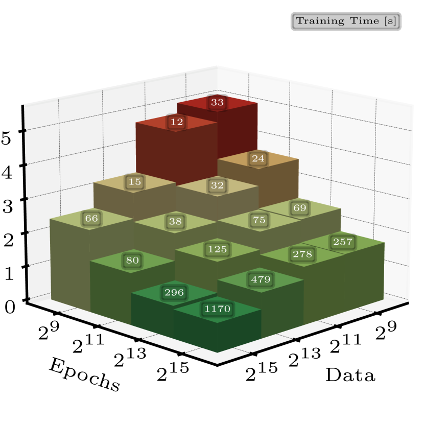
(a) Small Network

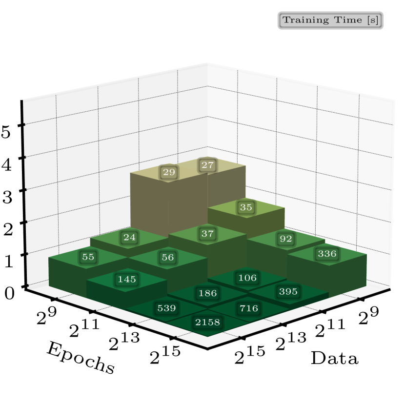
(b) Large Network

Figure 13: Data vs Epochs

Figures 13(a) demonstrates that even despite being a small model, the PINN-Small is capable of achieving errors as low as 1% given sufficient training data and training time. Even in the most data sparse conditions, the model remains able to converge to solutions with of than 5% error, and improve to values less than 1% given sufficient training time and data. Similarly, Figure 13(b) demonstrates that PINN-Large consistently benefits from additional training data and epochs, with the most accurate models reaching 0.04% error. Unlike the PINN-Small, the PINN-Large models always remained below 3% error even in the low data and epoch regimes. Taken together, the results of the large and small networks suggest that for optimal performance, the PINN-GM-III should be trained for at minimum 8,192 epochs but can still benefit from more if computing resources allow.

B.4 Data Quality and Physics Constraints

The final experiment investigates how the training data quality and physics constraints impact performance. This experiment begins by taking every acceleration vector and adding 10% of their magnitude in some random direction to the truth vector. This non-gaussian distribution is intended to stress these models and determine how well they converge on a true solution despite the error in the data. The experiment proceeds by training both the PINN-Small and PINN-Large on increasing amounts of training data ranging from $\{2^{9},2^{11},2^{13},2^{15}\}$. The experiment is performed once with the original augmented RMS / percent error loss function (PINN A)

$$\mathcal{L}_{\text{PINN A}}=\frac{1}{N}\sum^{N}_{i=0}\left(\sqrt{\left|-\nabla\hat{U}(\bm{x}_{i}|\mathbf{\theta})-\bm{a}_{i}\right|^{2}}+\frac{|-\nabla\hat{U}(\bm{x}_{i}|\mathbf{\theta})-\bm{a}_{i}|}{|\bm{a}_{i}|}\right)$$ (22)

and again with the Laplacian term added (PINN AL) or

$$\mathcal{L}_{\text{PINN AL}}=\frac{1}{N}\sum^{N}_{i=0}\left(\sqrt{\left|-\nabla\hat{U}(\bm{x}_{i}|\mathbf{\theta})-\bm{a}_{i}\right|^{2}}+\frac{|-\nabla\hat{U}(\bm{x}_{i}|\mathbf{\theta})-\bm{a}_{i}|}{|\bm{a}_{i}|}+\left|\nabla^{2}U(\bm{x}_{i})\right|\right)$$ (23)

Previously with the PINN-GM-II, adding the Laplacian constraint improved model performance when trained on noisy data martinSmallBodies2022 . This added considerable computational overhead the loss function, hence this experiment seeks to determine if this term remains necessary. Note that the batch size for this experiment is increased to $2^{15}$ to complete the test in a reasonable amount of training time, and the performance of the PINN-Large and PINN-Small models as a function of training data are provided in Figure 14.

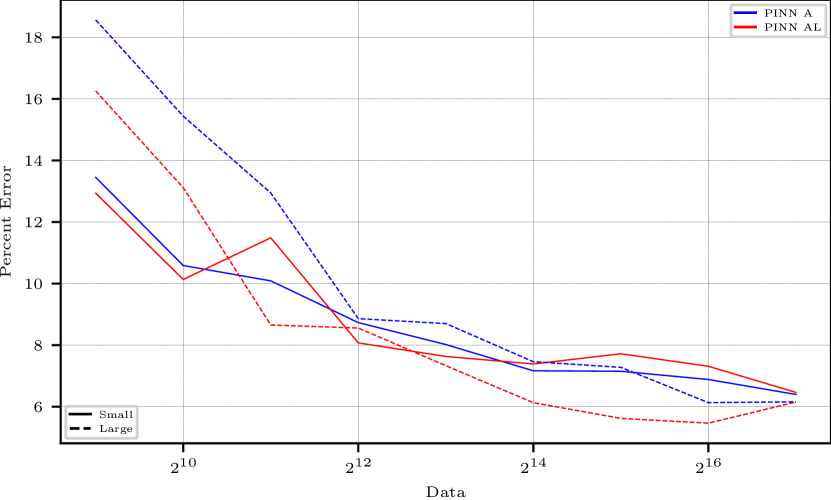
Figure 14: Error as a function of training data and loss function

Figure 14 shows that the noise in the training data does inevitably deteriorate model performance; however even with low quantities of training data, the PINN-GM Small is able to achieve errors as low as 13%, just slightly above the noise floor. As the amount of training data increases, the PINN-Small model reduces to approximately 7% error. The fact that these models are capable of regressing solutions beneath the noise floor is a testament to the physics-informed nature of these models. By leveraging the known dynamics of the system, the models can better ignore parts of the training data that are fundamentally inconsistent with the physics.

The PINN-Large is more susceptible to error in the low data regimes, reaching as high as 19% error in the 512 data point case. This is likely a manifestation of overfitting onto the limited training data given the model’s considerably higher parametric capacity than the PINN-Small model. In the PINN-Large model, the additional Laplacian component to the loss function (PINN AL) does improve the performance slightly, helping to regularize the model and minimizing its overfitting tendencies; however, in the small model the advantage is considerably less apparent. Given that the additional Laplacian constraint is far more computationally expensive than the simple PINN A constraint, it is generally advised to simply remain with the A constraint if in compute constrained settings.

Appendix C Comments on Past Machine Learning Performance

Table 1 highlights the general performance of past and present machine learning gravity models. All values are taken from their corresponding reference, but further context is warranted as each model assessed accuracy in different ways and on different asteroids. This section aims to provide relevant details regarding these metrics for completeness.

For the Gaussian process gravity model reported in Reference 26, the number of model parameters are not explicitly reported, but can be deduced. Gaussian processes are defined by their covariance matrix and kernel function. The covariance matrix scales as $\mathcal{O}(N^{2})$ and the maximum number of data points used were $N=3,600$. This suggests that the minimum number of parameters used in the model is 12,960,000. The accuracy for these models are also reported at fixed radii from the center of mass for each asteroid rather than across the full domain, so the values can be considered upper-bounds. Moreover, the model is shown to diverge at high altitudes hence is not valid globally.

For the extreme learning machine gravity model reported in Reference 28, the model size is determined by the fact that there are 50,000 hidden nodes in the ELM. The first 50,000 parameters constitute the random weights connecting the inputs to the hidden layer, and the second 50,000 parameters are the learned weights from the hidden layer to the output layer, totalling to 100,000 total model parameters. The asteroid modeled is 25143 Itokawa. The error in the Reference 28 is reported in terms of absolute terms rather than relative terms, however using Figure 9 it can be approximated that the relative error varies between 1% and 10%.

In Reference 31, the neural network gravity model is reported to use 512 nodes per hidden layer for 6 hidden layers ($512^{2}*6=1,572,864$ parameters). The paper reports 1,000,000 training data were generated and divided into an 8:2 ratio between training and testing data, totalling to 800,000 training data. The asteroid investigated is also 433-Eros and the average relative error of the test set is reported as 0.35% in their Table 3.

For GeodesyNets izzoGeodesyIrregularSmall2022 , SIRENs of 9 hidden layers with 100 nodes each are used (9*$100^{2}$ = 90,000). Four asteroids are studied: Bennu, Churyumov-Gerasimenko, Eros, and Itokawa. In their supplementary materials (Table S4), the relative error about Eros is reported at three characteristic altitudes. At their lowest altitude, the average error is 0.571% and their highest altitude is 0.146%. In attempts to quantify error across the entire high and low altitude regime, these values are averaged for the reported value of 0.359%.

Finally for the PINN-GM-III, the average error reported for a network trained with 8 hidden layers with 16 nodes per layer. The model was trained on 4,096 data points distributed between 0-10R using the same hyperparameters specified in Appendix B, and achieved an average error on the validation set of 0.3%.

Appendix D Regression Details

In Section 5, multiple gravity models are regressed and tested on a variety of data conditions. The regression procedure for the neural networks is consistent with prior explanations; however, the remaining models require further context. This section aims to provide that context, explaining how each of the remaining gravity models are regressed on the data discussed in Section 5.

D.1 Spherical Harmonics

Spherical harmonic gravity model are regressed by solving a linear system for their Stokes coefficients. This system takes the following form:

$$\bm{a} =H\bm{c}$$ (24)

$$H^{T}\bm{a} =H^{T}H\bm{c}$$ (25)

$$(H^{T}H)^{-1}H^{T}\bm{a} =\bm{c}$$ (26)

where $\bm{c}$ are the vector of spherical harmonic coefficients $C_{lm}$ and $S_{lm}$, $\bm{a}$ are the vector of accelerations, and $H$ is the jacobian $\frac{\partial\bm{a}}{\partial\bm{c}}|_{\bm{r}}$, and $\bm{r}$ is the position vector for each field point. Direct least square solutions may be appropriate for small systems, but as the size of the spherical harmonic model grows and the amount of data increases, this process quickly becomes computationally infeasible. Moreover, high-degree spherical harmonic models pose numerical instabilities as the observability of the harmonics decays rapidly as $(R/r)^{l}$, often making $H^{T}H$ ill-conditioned.

Multiple strategies exist to mitigate these concerns. One of the most popular is the use of Kaula’s rule, a form of ridge regression that can be used to regularize the spherical harmonic coefficients and assist in the ill-conditioned nature of the high-degree regression. Explicitly, rather than seeking to minimize the mean squared error solution

$$L(\bm{c})=|\bm{a}-H\bm{c}|^{2}$$ (27)

instead add a penalty term to ensure the coefficients decay in magnitude for higher degree harmonics through

$$L(\bm{c})=|\bm{a}-H\bm{c}|^{2}+|\Gamma\bm{c}|^{2}$$ (28)

where $\Gamma$ are the regularization matrix defined through Kaula’s rule

$$\Gamma_{ll}=\begin{cases}\frac{\alpha}{l^{2}}&l>0\\ 1&l=0\end{cases}$$ (29)

where $\alpha$ is a user specified constant typically chosen through cross validation. The corresponding solution to the ridge regression then becomes

$$(H^{T}H+\Gamma)^{-1}H^{T}\bm{a}=\bm{c}\\$$ (30)

which yields a solution with increasingly small spherical harmonic coefficients at high-degree. This simultaneously removes the ill-posed nature of the original regression and also provides a framework for supporting low-data regression.

While using Kaula’s rule mitigates the ill-posedness of the original regression, it remains computationally expensive to invert $(H^{T}H+\Gamma)$ for large datasets. This is solved with two strategies: 1) recursive least squares and 2) iterative coefficient regression. Recursive least square sequentially feeds in small batches of data to maintain computational tractability, while iterative coefficient regression regresses the low-degree harmonics separately from high-degree harmonics.

The recursive least squares is performed in batches of 100 position / acceleration pairs using the following recursion relationships

$$K_{i+1}^{-1} =K_{i}^{-1}-K_{i}^{-1}H_{k}^{T}(I+H_{k}K_{i}^{-1}H_{k}^{T})^{-1}H_{k}K_{i}^{-1}$$ (31)

$$\bm{c}_{k+1} =\bm{c}_{k}+K_{i+1}^{-1}H_{k}^{T}(\bm{a}_{k}-H_{k}\bm{c}_{k})$$ (32)

where $K_{0}^{-1}=(H_{0}^{T}H_{0}+\Gamma)^{-1}$, and the iterative coefficient regression is performed by only regressing 5,000 coefficients at a time.

The final note related to regressing the spherical harmonic model for the comparison study is that samples beneath the Brillouin surface $r<R$ are purposefully omitted from the regression due to the $(R/r)^{l}$ scaling in the harmonic model. For very high degree models, this term diverges when evaluated on sub-Brillouin samples, which breaks the regression.

D.2 Mascons

Like spherical harmonics, mascons regression is also a form of least squares regression. Specifically, a set of $N$ mascons are uniformly distributed through the volume of the shape model, and their corresponding masses are regressed. Ideally, the mascon regression should also include a non-linear constraint applied to all mass elements that ensures they always have a value greater than zero to ensure compliance with physics — i.e. there are no such things as negative masses. This physical compliance, however, often comes at a major loss of modeling accuracy. Therefore, Section 5 allows for negative masses to be regressed to give the model the strongest cases against the PINN-GM.

In addition to allowing negative masses, the mascon regression also requires iterative fitting when the model sizes are large and there exists much data. To do this, the mascons are distributed and fit in batches of 500 using all available data. After each batch is fit, their contribution to the acceleration vectors are removed, the next batch is randomly distributed throughout the volume, and the model fits to the acceleration residuals. This process is repeated until the total mass elements are reached.

D.3 Extreme Learning Machines

Extreme learning machines regression also closely resembles that of the spherical harmonic regression in that it also uses ridge regression and recursive least squares optimization. Explicitly, the ELM models are regressed by applying a fixed ridge regression matrix $\Gamma_{\text{ELM}}=\alpha\mathbb{I}$ and breaking the dataset into batches to be applied recursively using Eqs. 32. Notably, the ELM also relies on a random non-linear projection into a higher-dimensional space before the linear regression as described in detail in furfaroModelingIrregularSmall2020 . For the comparison study in this paper, all input and output data are preprocessed using a min-max transformation to $[0,1]$ and applying a sigmoid activation function at the hidden nodes.

References

- \bibcommenthead
- (1) Cuomo, S., di Cola, V.S., Giampaolo, F., Rozza, G., Raissi, M., Piccialli, F.: Scientific Machine Learning through Physics-Informed Neural Networks: Where We Are and What’s Next. arXiv (2022)
- (2) Karniadakis, G.E., Kevrekidis, I.G., Lu, L., Perdikaris, P., Wang, S., Yang, L.: Physics-informed machine learning. Nature Reviews Physics 3(6), 422–440 (2021). https://doi.org/10.1038/s42254-021-00314-5
- (3) Raissi, M., Perdikaris, P., Karniadakis, G.E.: Physics-informed neural networks: A deep learning framework for solving forward and inverse problems involving nonlinear partial differential equations. Journal of Computational Physics 378, 686–707 (2019). https://doi.org/10.1016/j.jcp.2018.10.045
- (4) Martin, J., Schaub, H.: Physics-informed neural networks for gravity field modeling of the Earth and Moon. Celestial Mechanics and Dynamical Astronomy 134(2) (2022). https://doi.org/10.1007/s10569-022-10069-5
- (5) Martin, J., Schaub, H.: Physics-Informed Neural Networks for Gravity Field Modeling of Small Bodies. Celestial Mechanics and Dynamical Astronomy, 28 (2022)
- (6) Brillouin, M.: équations aux dérivées partielles du 2e ordre. Domaines à connexion multiple. Fonctions sphériques non antipodes 4, 173–206 (1933)
- (7) Kaula, W.M.: Theory of Satellite Geodesy: Applications of Satellites to Geodesy. Blaisdell Publishing Co, Waltham, Mass. (1966)
- (8) Pavlis, N.K., Holmes, S.A., Kenyon, S.C., Schmidt, D., Trimmer, R.: A Preliminary Gravitational Model to Degree 2160. In: Gravity, Geoid and Space Missions vol. 129, pp. 18–23. Springer-Verlag, Berlin/Heidelberg (2005). https://doi.org/10.1007/3-540-26932-0_4
- (9) Goossens, S., Lemoine, F.~., Sabaka, T.~., Nicholas, J.~., Mazarico, E., Rowlands, D.~., Loomis, B.~., Chinn, D.~., Neumann, G.~., Smith, D.~., Zuber, M.~.: A Global Degree and Order 1200 Model of the Lunar Gravity Field Using GRAIL Mission Data. In: 47th Annual Lunar and Planetary Science Conference. Lunar and Planetary Science Conference, pp. 1484–1484 (2016)
- (10) Genova, A., Goossens, S., Lemoine, F.G., Mazarico, E., Neumann, G.A., Smith, D.E., Zuber, M.T.: Seasonal and static gravity field of Mars from MGS, Mars Odyssey and MRO radio science. Icarus 272, 228–245 (2016). https://doi.org/10.1016/j.icarus.2016.02.050
- (11) Gravity, G.: The Earth’s Gravitational Field 2.1 vol. 1, p. 64 (2016). https://doi.org/10.1002/14651858.CD000031.pub4.www.cochranelibrary.com
- (12) Hewitt, E., Hewitt, R.E.: The Gibbs-Wilbraham phenomenon: An episode in fourier analysis. Archive for History of Exact Sciences 21(2), 129–160 (1979). https://doi.org/10.1007/BF00330404
- (13) Martin, J.R., Schaub, H.: GPGPU Implementation of Pines’ Spherical Harmonic Gravity Model. In: Wilson, R.S., Shan, J., Howell, K.C., Hoots, F.R. (eds.) AAS/AIAA Astrodynamics Specialist Conference. Univelt Inc., Virtual Event (2020)
- (14) Werner, R., Scheeres, D.: Exterior gravitation of a polyhedron derived and compared with harmonic and mascon gravitation representations of asteroid 4769 Castalia. Celestial Mechanics and Dynamical Astronomy 65(3), 313–344 (1997). https://doi.org/10.1007/BF00053511
- (15) Scheeres, D.J., Khushalani, B., Werner, R.A.: Estimating asteroid density distributions from shape and gravity information. Planetary and Space Science 48(10), 965–971 (2000). https://doi.org/10.1016/s0032-0633(00)00064-7
- (16) Scheeres, D.J., French, A.S., Tricarico, P., Chesley, S.R., Takahashi, Y., Farnocchia, D., McMahon, J.W., Brack, D.N., Davis, A.B., Ballouz, R.L., Jawin, E.R., Rozitis, B., Emery, J.P., Ryan, A.J., Park, R.S., Rush, B.P., Mastrodemos, N., Kennedy, B.M., Bellerose, J., Lubey, D.P., Velez, D., Vaughan, A.T., Leonard, J.M., Geeraert, J., Page, B., Antreasian, P., Mazarico, E., Getzandanner, K., Rowlands, D., Moreau, M.C., Small, J., Highsmith, D.E., Goossens, S., Palmer, E.E., Weirich, J.R., Gaskell, R.W., Barnouin, O.S., Daly, M.G., Seabrook, J.A., Al Asad, M.M., Philpott, L.C., Johnson, C.L., Hartzell, C.M., Hamilton, V.E., Michel, P., Walsh, K.J., Nolan, M.C., Lauretta, D.S.: Heterogeneous mass distribution of the rubble-pile asteroid (101955) Bennu. Science Advances 6(41) (2020). https://doi.org/10.1126/sciadv.abc3350
- (17) Zuber, M.T., Smith, D.E., Cheng, A.F., Garvin, J.B., Aharonson, O., Cole, T.D., Dunn, P.J., Guo, Y., Lemoine, F.G., Neumann, G.A., Rowlands, D.D., Torrence, M.H.: The shape of 433 Eros from the NEAR-Shoemaker Laser Rangefinder. Science 289(5487), 2097–2101 (2000). https://doi.org/10.1126/science.289.5487.2097
- (18) Shepard, M.K., Timerson, B., Scheeres, D.J., Benner, L.A.M., Giorgini, J.D., Howell, E.S., Magri, C., Nolan, M.C., Springmann, A., Taylor, P.A., Virkki, A.: A revised shape model of asteroid (216) Kleopatra. Icarus 311, 197–209 (2018). https://doi.org/10.1016/j.icarus.2018.04.002
- (19) Miller, J.K., Konopliv, A.S., Antreasian, P.G., Bordi, J.J., Chesley, S., Helfrich, C.E., Owen, W.M., Wang, T.C., Williams, B.G., Yeomans, D.K., Scheeres, D.J.: Determination of shape, gravity, and rotational state of asteroid 433 Eros. Icarus 155(1), 3–17 (2002). https://doi.org/10.1006/icar.2001.6753
- (20) Romain, G., Jean-Pierre, B.: Ellipsoidal harmonic expansions of the gravitational potential: Theory and application. Celestial Mechanics and Dynamical Astronomy 79(4), 235–275 (2001). https://doi.org/10.1023/A:1017555515763
- (21) Takahashi, Y., Scheeres, D.J., Werner, R.A.: Surface gravity fields for asteroids and comets. Journal of Guidance, Control, and Dynamics 36(2), 362–374 (2013). https://doi.org/10.2514/1.59144
- (22) Takahashi, Y., Scheeres, D.J.: Small body surface gravity fields via spherical harmonic expansions. Celestial Mechanics and Dynamical Astronomy 119(2), 169–206 (2014). https://doi.org/10.1007/s10569-014-9552-9
- (23) Muller, A.P.M., Sjogren, W.L.: Mascons : Lunar Mass Concentrations 161(3842), 680–684 (1968)
- (24) Tardivel, S.: The Limits of the Mascons Approximation of the Homogeneous Polyhedron. In: AIAA/AAS Astrodynamics Specialist Conference, pp. 1–13. American Institute of Aeronautics and Astronautics, Reston, Virginia (2016). https://doi.org/10.2514/6.2016-5261
- (25) Wittick, P.T., Russell, R.P.: Mixed-model gravity representations for small celestial bodies using mascons and spherical harmonics. Celestial Mechanics and Dynamical Astronomy 131(7), 31–31 (2019). https://doi.org/10.1007/s10569-019-9904-6
- (26) Gao, A., Liao, W.: Efficient gravity field modeling method for small bodies based on Gaussian process regression. Acta Astronautica 157(December 2018), 73–91 (2019). https://doi.org/10.1016/j.actaastro.2018.12.020
- (27) Cheng, L., Wang, Z., Jiang, F.: Real-time control for fuel-optimal Moon landing based on an interactive deep reinforcement learning algorithm. Astrodynamics 3(4), 375–386 (2019). https://doi.org/10.1007/s42064-018-0052-2
- (28) Furfaro, R., Barocco, R., Linares, R., Topputo, F., Reddy, V., Simo, J., Le Corre, L.: Modeling irregular small bodies gravity field via extreme learning machines and Bayesian optimization. Advances in Space Research (June) (2020). https://doi.org/10.1016/j.asr.2020.06.021
- (29) Izzo, D., Gómez, P.: Geodesy of irregular small bodies via neural density fields. Communications Engineering 1(1), 48 (2022). https://doi.org/10.1038/s44172-022-00050-3
- (30) Huang, G.-B., Zhu, Q.-Y., Siew, C.-K.: Extreme learning machine: Theory and applications. Neurocomputing 70(1-3), 489–501 (2006). https://doi.org/10.1016/j.neucom.2005.12.126
- (31) Cheng, L., Wang, Z., Song, Y., Jiang, F.: Real-time optimal control for irregular asteroid landings using deep neural networks. Acta Astronautica 170(January 2019), 66–79 (2020). https://doi.org/10.1016/j.actaastro.2019.11.039
- (32) Kingma, D.P., Ba, J.: Adam: A Method for Stochastic Optimization. 3rd International Conference on Learning Representations, ICLR 2015 - Conference Track Proceedings, 1–15 (2014)
- (33) Dozat, T.: Incorporating Nesterov Momentum into Adam
- (34) Nocedal, J., Wright, S.J.: Numerical Optimization, 2nd ed edn. Springer Series in Operations Research. Springer, New York (2006)
- (35) Mildenhall, B., Srinivasan, P.P., Tancik, M., Barron, J.T., Ramamoorthi, R., Ng, R.: NeRF: Representing scenes as neural radiance fields for view synthesis. Communications of the ACM 65(1), 99–106 (2022). https://doi.org/10.1145/3503250
- (36) Baydin, A.G., Pearlmutter, B.A., Siskind, J.M.: Automatic Differentiation in Machine Learning: A Survey. Journal of Machine Learning Research 18, 1–43 (2018)
- (37) Martin, J.R., Schaub, H.: Preliminary Analysis of Small-Body Gravity Field Estimation using Physics-Informed Neural Networks and Kalman Filters. th International Astronautical Congress, 10 (2022)
- (38) Goodfellow, I., Bengio, Y., Courville, A.: Deep Learning. MIT Press, ??? (2016)
- (39) Pines, S.: Uniform Representation of the Gravitational Potential and its Derivatives. AIAA Journal 11(11), 1508–1511 (1973). https://doi.org/10.2514/3.50619
- (40) Zhu, Q., Liu, Z., Yan, J.: Machine Learning for Metal Additive Manufacturing: Predicting Temperature and Melt Pool Fluid Dynamics Using Physics-Informed Neural Networks. arXiv (2020)
- (41) Takahashi, Y., Scheeres, D.J.: Morphology driven density distribution estimation for small bodies. Icarus 233, 179–193 (2014). https://doi.org/10.1016/j.icarus.2014.02.004
- (42) KANAMARU, M., SASAKI, S.: Estimation of Interior Density Distribution for Small Bodies: The Case of Asteroid Itokawa. Transactions of the Japan Society for Aeronautical and Space Sciences, Aerospace Technology Japan 17(3), 270–275 (2019). https://doi.org/10.2322/tastj.17.270
- (43) Hendrycks, D., Gimpel, K.: Gaussian Error Linear Units (GELUs). arXiv (2020)