On selecting a fraction of leaves with disjoint neighborhoods in a plane tree

Abstract

We present a generalization of a combinatorial result by Aggarwal, Guibas, Saxe and Shor [Discrete & Computational Geometry, 1989] on a linear-time algorithm that selects a constant fraction of leaves, with pairwise disjoint neighborhoods, from a binary tree embedded in the plane. This result of Aggarwal et al. is essential to the linear-time framework, which they also introduced, that computes certain Voronoi diagrams of points with a tree structure in linear time. An example is the diagram computed while updating the Voronoi diagram of points after deletion of one site. Our generalization allows that only a fraction of the tree leaves is considered, and it is motivated by linear-time Voronoi constructions for non-point sites. We are given a plane tree $T$ of $n$ leaves, $m$ of which have been marked, and each marked leaf is associated with a neighborhood (a subtree of $T$) such that any two topologically consecutive marked leaves have disjoint neighborhoods. We show how to select in linear time a constant fraction of the marked leaves having pairwise disjoint neighborhoods.

1 Introduction

In 1987, Aggarwal, Guibas, Saxe and Shor [1] introduced a linear-time technique to compute the Voronoi diagram of points in convex position, which can also be used to compute other Voronoi diagrams of point-sites with a tree structure such as: (1) updating a nearest-neighbor Voronoi diagram of points after deletion of one site; (2) computing the farthest-point Voronoi diagram, after the convex hull of the points is known; (3) computing an order-$k$ Voronoi diagram of points, given its order-($k\textup{-}1$) counterpart. Since then, this framework has been used (and extended) in various ways to tackle various linear-time Voronoi constructions, including the medial axis of a simple polygon by Chin et al. [4], the Hamiltonian abstract Voronoi diagram by Klein and Lingas [8], and some forest-like abstract Voronoi diagrams by Bohler et al. [2]. The linear-time construction for problem (3) improves by a logarithmic factor the standard iterative construction by Lee [9] to compute the order-k Voronoi diagram of point-sites, which is in turn used in different scenarios; for example, algorithms for coverage problems in wireless networks by So and Ye [10]. A much simpler randomized linear-time approach for problems (1)-(3) was introduced by Chew [3].

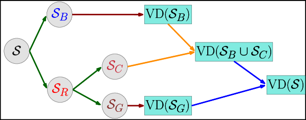
Figure 1: The divide & conquer algorithm of [1]. ($\longrightarrow$) indicates the two different divide phases; ($\longrightarrow$) indicates the recursive constructions; ($\longrightarrow$) indicates site insertion; ($\longrightarrow$) indicates merging.

The linear-time technique of Aggarwal et al. [1] is a doubly-recursive divide-and-conquer scheme operating on an ordered set of points $S$ whose Voronoi diagram is a tree with connected Voronoi regions. At a high level it can be described as follows, see Figure 1. In an initial divide phase, the set $S$ is split in two sets $\mathcal{S}_{R}$ (red) and $\mathcal{S}_{B}$ (blue) of roughly equal size, with the property that every two consecutive red sites in $\mathcal{S}_{R}$ have disjoint Voronoi regions. In a second divide phase, the set $\mathcal{S}_{R}$ is split further in sets $\mathcal{S}_{C}$ (crimson) and $\mathcal{S}_{G}$ (garnet), so that any two sites in $\mathcal{S}_{C}$ have pairwise disjoint regions in the Voronoi diagram of $\mathcal{S}_{B}\cup\mathcal{S}_{C}$, and the cardinality of $\mathcal{S}_{C}$ is a constant fraction of the cardinality of $\mathcal{S}_{R}$. In the merge phase, the sites of $\mathcal{S}_{C}$ are inserted one by one in the recursively computed Voronoi diagram of $\mathcal{S}_{B}$, deriving the Voronoi diagram of $\mathcal{S}_{C}\cup\mathcal{S}_{B}$, and the result is merged with the recursively computed diagram of $\mathcal{S}_{G}$.

The key factor in obtaining the linear-time complexity is that the cardinality of the set $\mathcal{S}_{C}$ is a constant fraction of $\mathcal{S}_{R}$, which is $\Theta(\mathcal{|S|})$, and that $\mathcal{S}_{C}$ can be obtained in linear time. This is possible due to the following combinatorial result of [1] on a geometric binary tree embedded in the plane. This result is, thus, inherently used by any algorithm that is based on the linear-time framework of Aggarwal et al. A binary tree that contains no nodes of degree 2 is called proper.

Theorem 1 ([1]).

Let $\mathcal{T}$ be an unrooted (proper) binary tree embedded in the plane. Each leaf of $\mathcal{T}$ is associated with a neighborhood, which is a (proper) subtree of $\mathcal{T}$ rooted at that leaf; consecutive leaves in the topological ordering of $\mathcal{T}$ have disjoint neighborhoods. Then, there exists a fixed fraction of the leaves whose neighborhoods are pairwise disjoint, they have a constant size, and no tree edge has its endpoints in two different neighborhoods. Such a set of leaves can be found in linear time.

Overall, the time complexity of the algorithm is described by the following recursive equation and can be proved to be $\Theta(n)$, where $n=|\mathcal{S}|$.

$$T(n)= \ T(|\mathcal{S}_{B}|)+T(|\mathcal{S}_{G}|)+\Theta(|\mathcal{S}_{R}|)+|\mathcal{S}_{C}|\cdot\Theta(1)+\Theta(n)$$

$$= \ T(|\mathcal{S}_{B}|)+T(|\mathcal{S}_{G}|)+\Theta(n)$$

$$= \ \Theta(n) |\mathcal{S}_{C}|=\Theta(n)$$ (Because )

It is worth understanding what Theorem 1 represents, in order to have a spherical perspective of its connection to Voronoi diagrams. An embedded tree corresponds to the graph structure of a Voronoi diagram, and leaves are the endpoints of unbounded Voronoi edges ”at infinity”; see Figure 2(a). The neighborhood of a leaf corresponds to the part of the diagram (of $\mathcal{S}_{B}$) that gets deleted if a point-site is inserted there; see Figure 2(b). Hence, Theorem 1 aims to select leaves with pairwise disjoint neighborhoods ($\mathcal{S}_{C}$), as they can easily, and independently from one another, be inserted in the diagram.

(a) The Voronoi diagram of 5 points ($\sqbullet$); the neighborhood of $\ell_{2}$ is shaded.

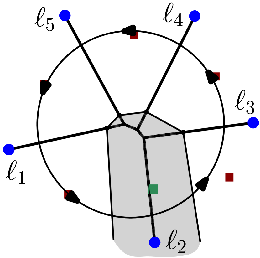
(b) The dashed part of the diagram will get deleted if point ($\sqbullet$) is inserted.

(c) The topological ordering of the leaves in $\mathcal{T}$.

Figure 2: An embedded binary tree $\mathcal{T}$ in the setting of Aggarwal et al. [1].

For generalized sites, other than points in the plane, or for abstract Voronoi diagrams, deterministic linear-time algorithms for the counterparts of problems (1)-(3) have not been known so far. This includes the diagrams of very simple geometric sites such as line segments and circles in the Euclidean plane. A major complication over points is that the underlying diagrams have disconnected Voronoi regions. Recently Papadopoulou et al. [6, 7] presented a randomized linear-time technique for these problems, based on a relaxed Voronoi structure, called a Voronoi-like diagram [6, 7]. Whether this structure can be used within the framework of Aggarwal et al., leading to deterministic linear-time constructions, remains still an open problem. Towards resolving this problem we need a generalized version of Theorem 1.

The problem is formulated as follows. We have an unrooted binary tree $\mathcal{T}$ embedded in the plane, which corresponds to a Voronoi-like structure. Not all leaves of $\mathcal{T}$ are eligible for inclusion in the set ${S_{C}}$ of the linear-time framework. As in the original problem, each of the eligible leaves is associated with a neighborhood, which is a subtree of $\mathcal{T}$ rooted at that leaf, and adjacent leaves in the topological ordering of $\mathcal{T}$ have disjoint neighborhoods. In linear time, we need to compute a constant fraction of the eligible leaves such that their neighborhoods are pairwise disjoint. The non-eligible leaves spread arbitrarily along the topological ordering of the tree leaves. This paper addresses this problem by proving the following generalization of Theorem 1.

Theorem 2.

Let $\mathcal{T}$ be an unrooted (proper) binary tree embedded in the plane having $n$ leaves, $m$ of which have been marked. Each marked leaf of $\mathcal{T}$ is associated with a neighborhood, which is a proper subtree of $\mathcal{T}$ rooted at this leaf, and any two consecutive marked leaves in the topological ordering of $\mathcal{T}$ have disjoint neighborhoods. Then, there exist at least $\frac{1}{10}m$ marked leaves whose neighborhoods are pairwise disjoint and no tree edge has its endpoints in two of these neighborhoods. Further, we can select at least a fraction $p$ of these $\frac{1}{10}m$ marked leaves in time $O(\frac{1}{1-p}n)$, for any $p\in(0,1)$.

The algorithm of Theorem 2 allows for a trade-off between the number of the returned marked leaves and its time complexity, using a parameter $p\in(0,1)$. If $p$ is constant then the algorithm returns a constant fraction of the marked leaves in $O(n)$ time. Theorem 2 is a combinatorial result on an embedded tree, and thus, we expect it to find applications in different contexts as well.

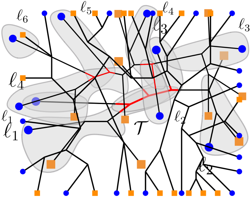
(a) Neighborhoods of the marked leaves are shown shaded. The intersection of neighborhoods is highlighted with red.

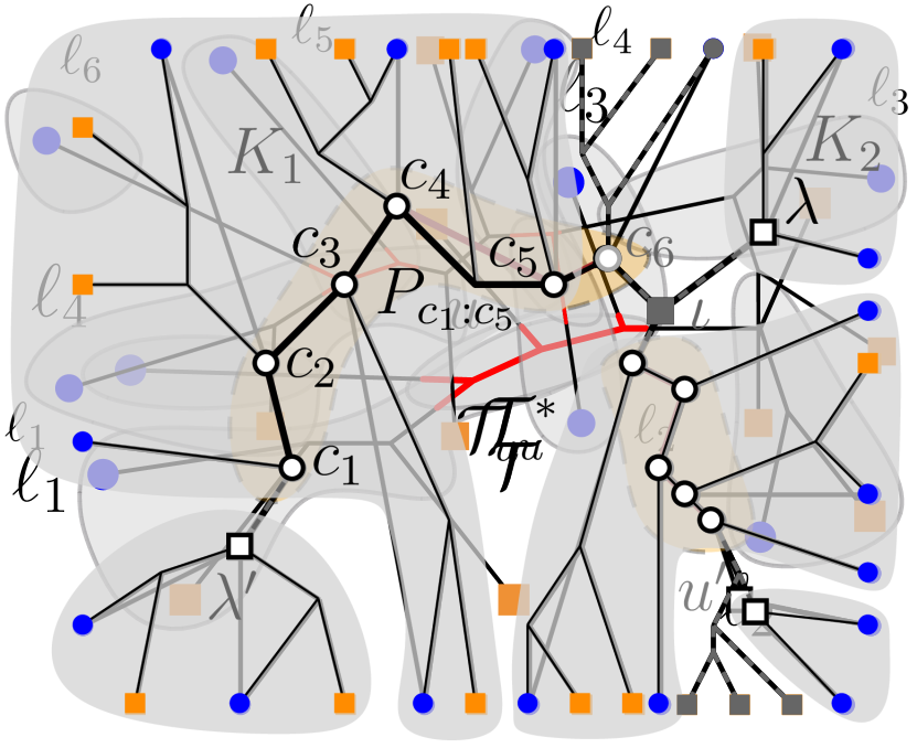
(b) A marked tree $\mathcal{T}$, which serves as an example instance for illustrating the notions of Section 2.

Figure 3: Two marked trees, where marked leaves are shown with ($\bullet$) and unmarked leaves are shown with ($\sqbullet$).

2 Preliminaries

Throughout this work, we consider an unrooted binary tree $\mathcal{T}$ of $n$ leaves that is embedded in the plane. The tree $\mathcal{T}$ contains no nodes of degree 2 and has the following additional properties:

1. $m$ out of the $n$ leaves of $\mathcal{T}$ have been marked, and the remaining $r=n{-}m$ leaves are unmarked (see Figure 3(b)).

2. Every marked leaf $\ell$ is associated with a neighborhood, denoted $nh(\ell)$, which is a subtree of $\mathcal{T}$ rooted at $\ell$ (see Figure 3(a)).

3. Every two consecutive marked leaves in the topological ordering of $\mathcal{T}$ have disjoint neighborhoods (see Figure 3(a)).

We call a binary tree $\mathcal{T}$ that follows these properties, a marked tree. Given a marked tree $\mathcal{T}$, let $\mathcal{T}_{u}$ denote the unmarked tree obtained by deleting all the unmarked leaves of $\mathcal{T}$ and contracting the resulting degree-$2$ nodes, see Figure 4(a). We apply to $\mathcal{T}_{u}$ the following definition, which is extracted from the proof of Theorem 1 in [1], see Figure 4.

Definition 1.

Let $T$ be a proper binary tree and let $T^{*}$ be the tree obtained from $T$ after deleting all its leaves. A node $u$ in $T^{*}$ is called:

1. Leaf or $L$-node if $deg(u)=1$ in $T^{*}$, i.e., $u$ neighbors two leaves in $T$.

2. Comb or $C$-node if $deg(u)=2$ in $T^{*}$, i.e., $u$ neighbors one leaf in $T$.

3. Junction or $J$-node if $deg(u)=3$ in $T^{*}$, i.e., $u$ neighbors no leaves in $T$.

A spine is a maximal sequence of consecutive $C$-nodes, which is delimited by $J$- or $L$-nodes. Each spine has two sides and marked leaves may lie in either side of a spine.

(a) Tree $\mathcal{T}_{u}$.

(b) Tree $\mathcal{T}_{u}^{*}$: $L$-nodes are shown with ($\square$), $C$-nodes with ($\circ$), $J$-nodes with ($\sqbullet$), and spines are highlighted.

Figure 4: Illustration of Definition 1 applied to the tree $\mathcal{T}$ of Figure 3(b).

Let $\mathcal{T}_{u}^{*}$, be the tree obtained by applying Definition 1 to the unmarked tree $\mathcal{T}_{u}$. The nodes $\mathcal{T}_{u}^{*}$ are labeled as $L$-, $C$- and $J$-nodes, see, e.g., Figure 4(b). The labeling of nodes in $\mathcal{T}_{u}^{*}$ is then carried back to their corresponding nodes in the original marked tree $\mathcal{T}$ obtaining a marked tree $\mathcal{T}$ with labels, see Figure 6. Some nodes in $\mathcal{T}$ remain unlabeled, see, e.g., node $u$ in Figure 6.

Definition 2.

Given a marked tree $\mathcal{T}$ with labels we define the following two types of components:

1. $L$-component: an $L$-node $\lambda$ defines an $L$-component that consists of $\lambda$ union the two subtrees of $\mathcal{T}$ that are incident to $\lambda$ and contain no labeled node, see, e.g., $K_{2}$ in Figure 6. The $L$-component contains exactly the two marked leaves that labeled $\lambda$.

2. $5$-component: a group of five successive $C$-nodes $c_{i},\dots,c_{i+4}$ on a spine defines a $5$-component that consists of the path $P_{c_{i}:c_{i+4}}$ from $c_{i}$ to $c_{i+4}$ (which may contain unlabeled nodes) union the subtrees of $\mathcal{T}$, which are incident to the nodes of $P_{c_{i}:c_{i+4}}$ and contain no labeled node, see, e.g., $K_{1}$ in Figure 6. Nodes $c_{i}$ and $c_{i+4}$ are referred to as the extreme nodes of $K$. The $5$-component contains exactly the five marked leaves, which labeled the five $C$-nodes.

Each spine is partitioned into consecutive groups of $5$-components and at most four remaining ungrouped $C$-nodes.

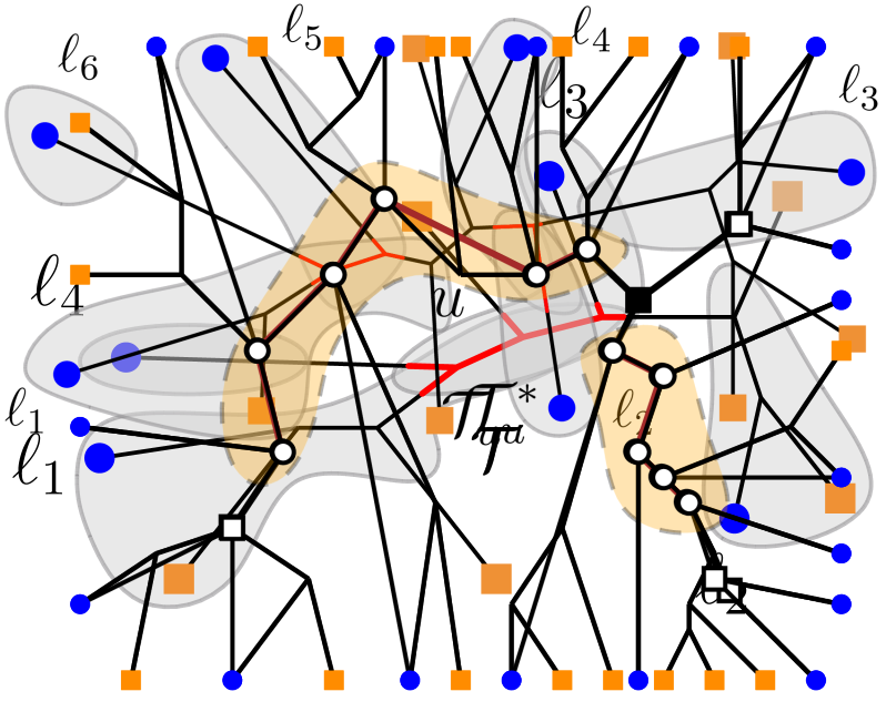
Figure 5: The marked tree $\mathcal{T}$ of Figure 3(b) with labels ($\circ$, $\square$, $\sqbullet$). Node $u$ is not labeled.

Figure 6: The components of $\mathcal{T}$ shown shaded. The dashed parts do not belong to any component.

Figure 6 and Figure 6 illustrates these definitions. The tree $\mathcal{T}$ has three $L$-components and two $5$-components which are indicated shaded in Figure 6. The $5$-component $K_{1}$ contains the path $P_{c_{1}:c_{5}}$ from $c_{1}$ to $c_{5}$, which is shown in thick black lines, and contains one unlabeled node. Node $c_{6}$ is an ungrouped $C$-node. Figure 6 also illustrates a spine consisting of the $C$-nodes $c_{1},c_{2},c_{3},c_{4},c_{5},c_{6}$. The spine is delimited by the $L$-node $\lambda^{\prime}$ and the $J$-node $\iota$; it has five marked leaves from one side and one marked leaf from the other.

Observation 1.

The components of $\mathcal{T}$ are pairwise vertex disjoint. Every $L$-component contains exactly two marked leaves and every $5$-component contains exactly five marked leaves.

Among the components of $\mathcal{T}$ there may be subtrees of $\mathcal{T}$ consisting of unlabeled nodes and unmarked leaves that may be arbitrarily large. These subtrees hang off any unlabeled nodes and ungrouped $C$-nodes. For example, in Figure 6, node $u^{\prime}$ is unlabeled and the gray dotted subtree incident to it consists solely of unmarked leaves and unlabeled nodes that do not belong to any component.

3 Existence of leaves with pairwise disjoint neighborhoods

Aggarwal et al. [1] showed that for every eight ungrouped $C$-nodes in $\mathcal{T}_{u}$ there exists at least one $L$-node. Their argument holds for the marked tree $\mathcal{T}$ as well, which is described in the following lemma for completeness.

Lemma 1.

For every eight ungrouped $C$-nodes in $\mathcal{T}$ there exists at least one $L$-component.

Proof.

We count the $L$-nodes of $\mathcal{T}$ using the tree $\mathcal{T}_{u}^{*}$ following the argument of [1]. Let $k$ be the number of leaves in $\mathcal{T}_{u}^{*}$, which also equals the number of $L$-nodes in $\mathcal{T}$. Contracting all degree-2 vertices in $\mathcal{T}_{u}^{*}$ yields a binary tree $\mathcal{T}_{b}^{*}$, which has the same leaves as $\mathcal{T}_{u}^{*}$. Since $\mathcal{T}_{b}^{*}$ is an unrooted binary tree with $k$ leaves, it has $2k-2$ nodes and $2k-3$ edges. Every edge in $\mathcal{T}_{b}^{*}$ corresponds to at most one spine in $\mathcal{T}_{u}^{*}$ and in every spine there are at most four ungrouped $C$-nodes. Thus,

$$|\text{ungrouped }C\text{-nodes}|\leq 4|\text{spines}|\leq 4\cdot(2k-3)<8|L\text{-nodes}|,$$

where $|\cdot|$ denotes cardinality. So, there exists at least one $L$-node for every eight ungrouped $C$-nodes, and an $L$-node corresponds to exactly one $L$-component. ∎

The following lemmata establish that there exists a constant fraction of the marked leaves, which have pairwise disjoint neighborhoods. The counting arguments follow those in [1] while they are further enhanced to account for the unmarked leaves, which are arbitrarily distributed among the marked leaves. We say that the neighborhood $nh(\ell)$ of a marked leaf $\ell$ is confined to a component $K$ if it is a subtree of $K$.

(a) An $L$-component

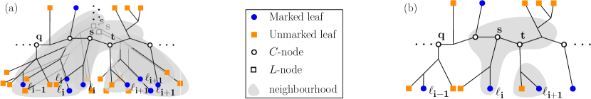
(b) A $5$-component

Figure 7: Marked leaves with their neighborhoods shaded. The neighborhood ${nh}(\ell_{i})$ is confined to the component in both cases.

Lemma 2.

In every component $K$, there exists a marked leaf $\ell\in K$ whose neighborhood is confined to $K$. This neighborhood may contain no $L$-node and no extreme $C$-node.

Proof.

Let $K$ be an $L$-component and let $s$ be the $L$-node that defines $K$. Let $\ell_{i}$ and $\ell_{i+1}$ be the two marked leaves of $K$. Since the neighborhoods $nh(\ell_{i})$ and $nh(\ell_{i+1})$ are disjoint, at least one of them cannot contain $s$. This neighborhood is, thus, entirely contained in the relevant subtree rooted at $s$, see Figure 7(a), and contains no labeled node.

Let $K$ be a $5$-component. Since a $5$-component has two sides, at least three out of the five marked leaves of the component must lie on the same side of $K$, call them $\ell_{i-1},\ell_{i}$ and $\ell_{i+1}$. Let $q,s$, and $t$ be their corresponding $C$-nodes, i.e., the first $C$-nodes in $K$ reachable from $\ell_{i-1},\ell_{i}$, and $\ell_{i+1}$, respectively, see Figure 7(b). There are three cases. If $t\in nh(\ell_{i})$, then $t\notin nh(\ell_{i+1})$ (since the two neighborhoods are disjoint), and thus, $nh(\ell_{i+1})$ is confined to the subtree of $t$ that contains $\ell_{i+1}$. Similarly, if $q\in nh(\ell_{i})$, then $q\notin nh(\ell_{i-1})$, so $nh(\ell_{i-1})$ is confined to the subtree of $q$ containing $\ell_{i-1}$. If neither $q$ nor $t$ are in $nh(\ell_{i})$, then clearly $nh(\ell_{i})$ is confined to $K$. In all cases the confined neighborhood cannot contain neither $q$ nor $t$. So, at least one of the five marked leaves must have a neighborhood confined to $K$ and this neighborhood cannot contain the extreme $C$-nodes in $K$. ∎

Lemma 3.

Let $\mathcal{T}$ be a marked tree with $m$ marked leaves. At least $\frac{1}{10}m$ marked leaves must have pairwise disjoint neighborhoods such that no tree edge may have its endpoints in two different neighborhoods.

Proof.

Every spine of $\mathcal{T}$ has up to four ungrouped $C$-nodes. By Lemma 1, there exists at least one $L$-component for every eight ungrouped $C$-nodes. By Lemma 2, every component of $\mathcal{T}$ has at least one marked leaf whose neighborhood is confined to the component. So, overall, at least $\frac{1}{5}$ of the marked leaves from each $5$-component and at least $\frac{1}{10}$ marked leaves of the remaining nodes, which label ungrouped $C$-nodes or $L$-nodes, have a confined neighborhood. The components are pairwise disjoint, so at least $\frac{1}{10}$ marked leaves have pairwise disjoint neighborhoods. Furthermore, confined neighborhoods do not contain any $L$-node or extreme $C$-node, as shown in Lemma 2. Thus, no tree edge may have its endpoints in two different neighborhoods. ∎

We remark that the neighborhoods implied by Lemma 3 may not contain any $L$-node nor any extreme $C$-node. We also remark that these neighborhoods need not be of constant complexity as their counterparts in [1] are. These neighborhoods may have complexity $\Theta(r)$, where $r=n-m$ is the number of unmarked leaves. Since $r$ may be $\Theta(n)$, this poses a challenge on how we can select these leaves efficiently.

4 Selecting leaves with pairwise disjoint neighborhoods

Given a marked tree $\mathcal{T}$ with $m$ marked leaves, we have already established the existence of $\frac{1}{10}m$ marked leaves that have pairwise disjoint neighborhoods. In this section, we present an algorithm to select a fraction $p$ of these leaves, i.e., $\frac{p}{10}m$ marked leaves with pairwise disjoint neighborhoods, in time $O(\frac{1}{1-p}n)$, where $0<p<1$.

The main challenge over the algorithm of [1] is that the $r$ unmarked leaves are arbitrarily distributed among the $m$ marked leaves, and thus, the components of $\mathcal{T}$ and the neighborhoods of the marked leaves may have complexity $\Theta(r)$. If for each component we spend time proportional to its size, then the time complexity of the algorithm will be $\Theta(mr)$, i.e., $\Theta(n^{2})$ if $r,m\in\Theta(n)$.

To keep the complexity of the algorithm linear, we spend time up to a predefined number of steps in each component depending on the ratio $c=\left\lceil\frac{r}{m}\right\rceil$ and the trade-off parameter $p\in(0,1)$. Our algorithm guarantees to find at least a fraction $p$ of the possible $\frac{1}{10}m$ marked leaves in time $O(\frac{1}{1-p}n)$. We first present a series of results necessary to establish the correctness of the approach and then describe the algorithm.

Let $\ell_{1},\dots,\ell_{m}$ be the marked leaves in $\mathcal{T}$ ordered in a counterclockwise topological ordering. Let the interval $(\ell_{i},\ell_{i+1})$ denote the set of unmarked leaves between $\ell_{i}$ and $\ell_{i+1}$ in the same order. The interval tree of $(\ell_{i},\ell_{i+1})$, denoted $T_{(\ell_{i},\ell_{i+1})}$, is the minimal subtree of $\mathcal{T}$ that contains the marked leaves $\ell_{i}$ and $\ell_{i+1}$, including the unmarked leaves in $(\ell_{i},\ell_{i+1})$, see Figure 8(b). We show the following pigeonhole lemma involving unmarked leaves and intervals.

Lemma 4.

Suppose that $r$ items (unmarked leaves) are distributed in $k\geq m$ containers (intervals), and let $c=\left\lceil\frac{r}{m}\right\rceil$. For any natural number $x\leq r$, let $k_{x}$ denote the number of containers that contain more than $x$ items. Then $k_{x}\leq\displaystyle\frac{cm}{x+1}$.

Proof.

Each of the $k_{x}$ containers contains at least $x+1$ items. Thus,

$$k_{x}(x+1)\leq r\ \Rightarrow\ k_{x}\ \leq\ \frac{r}{x+1}.$$ (1)

$$c\ =\ \displaystyle\left\lceil\frac{r}{m}\right\rceil\ \Rightarrow\ c\geq\ \frac{r}{m}\ \Rightarrow\ r\ \leq\ cm$$ (2)

$$(\ref{eq1})\stackrel{{\scriptstyle(\ref{eq2})}}{{\Longrightarrow}}\ k_{x}\ \leq\ \frac{cm}{x+1}$$ (3)

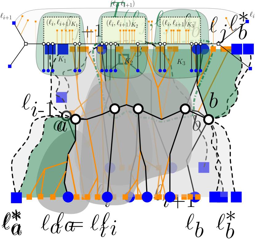
(a) An $L$-component.

(b)  A $5$-component with $\ell_{i}=\ell_{a}$. The interval tree $T_{(\ell_{j},\ell_{j+1})}$ is highlighted.

(c) A $5$-component with $\ell_{i}\notin\{\ell_{a},\ell_{b}\}$. The interval trees $T_{(\ell_{a},\ell_{a}^{*})}$ and $T_{(\ell_{b},\ell_{b}^{*})}$ are highlighted

Figure 8: Illustration of a component $K$ in different settings for the proof of Lemma 5. The neighborhood $nh(\ell_{i})$ is shaded gray. Marked leaves of $K$ are indicated with ($\bullet$) and the other marked leaves with ($\sqbullet$).

For a component $K$, let $\delta_{K}$ denote the maximum number of topologically consecutive unmarked leaves in $K$. The unmarked leaves counted in $\delta_{K}$ belong to some interval $(\ell_{i},\ell_{i+1})$.

Lemma 5.

Let $K$ be a component of $\mathcal{T}$ and let $\ell_{i}$ be a marked leaf whose neighborhood $nh(\ell_{i})$ is confined to $K$.

1. If $K$ is an $L$-component, then $nh(\ell_{i})$ has at most $4\delta_{K}$ nodes.

2. If $K$ is a $5$-component, then $nh(\ell_{i})$ has at most $10\delta_{K}$ nodes.

Proof.

Let $K$ be an $L$-component whose $L$-node is $s$, see Figure 8(a). Since $nh(\ell_{i})$ is confined to $K$ then $s\notin nh(\ell_{i})$. Thus, $s$ disconnects $nh(\ell_{i})$ from the rest of $\mathcal{T}$, making $nh(\ell_{i})$ disjoint from any interval tree, other than $T_{(\ell_{i-1},\ell_{i})}$ and $T_{(\ell_{i},\ell_{i+1})}$. Hence, $nh(\ell_{i})$ contains at most $2\delta_{K}+1$ leaves, and since it is a proper binary tree, it can have at most $4\delta_{K}$ nodes in total.

Suppose $K$ is a $5$-component. Since $K$ contains exacly five marked leaves, there can be at most seven interval trees that may share a node with $K$. Let $a$ and $b$ be the two extreme $C$-nodes of $K$ and let $\ell_{a}$ and $\ell_{b}$ be their corresponding marked leaves, which labeled $a$ and $b$ as $C$-nodes. Let $\ell_{a}^{*}$ (resp. $\ell_{b}^{*})$ be the neighboring marked leaf of $\ell_{a}$ (resp. $\ell_{b})$ in the topological ordering of the marked leaves, which does not belong to $K$. Refer to Figure 8(b) and Figure 8(c). Neighborhood $nh(\ell_{i})$ is confined to $K$, thus, $a,b\notin nh(\ell_{i})$. If $\ell_{i}=\ell_{a}$ (resp. $\ell_{i}=\ell_{b}$) the $C$-node $a$ (resp. $b$), disconnects $nh(\ell_{i})$ from the rest of $\mathcal{T}$. Thus, $nh(\ell_{i})$ has a node in common with only two interval trees, $T_{(\ell_{i-1},\ell_{i})}$ and $T_{(\ell_{i},\ell_{i+1})}$, see Figure 8(b). If $\ell_{i}\notin\{\ell_{a},\ell_{b}\}$, then nodes $a$ and $b$ disconnect $nh(\ell_{i})$ from the rest of $\mathcal{T}$, thus, $nh(\ell_{i})$ is disjoint from both $T_{(\ell_{a},\ell_{a}^{*})}$ and $T_{(\ell_{b},\ell_{b}^{*})}$, see Figure 8(c). Then $nh(\ell_{i})$ may have a node in common with at most five out of the seven interval trees that could be related to $K$. Concluding, $nh(\ell_{i})$ has at most $5\delta_{K}+1$ leaves, and since it is a proper binary tree, it has at most $10\delta_{K}$ nodes overall. ∎

For each component $K$ we define a so-called representative leaf and at most two delimiting nodes. These are used by our algorithm to identify a confined neighborhood within the component.

Definition 3.

For a component $K$, we define its representative leaf and delimiting nodes as follows:

1. If $K$ is an $L$-component, there is one delimiting node, which is its $L$-node. The representative leaf is the first marked leaf of $K$ in the topological ordering of leaves. In Figure 7(a), $\ell_{i}$ is the representative leaf and $s$ is the delimiting node.

2. If $K$ is a $5$-component, consider the side of $K$ containing at least three marked leaves. The representative leaf is the second leaf among these three leaves in the topological ordering. The delimiting nodes are the $C$-nodes defined by the other two leaves in the same side. In Figure 7(b), $\ell_{i}$ is the representative leaf and $q,t$ are the delimiting nodes.

Our algorithm takes as input a marked tree $\mathcal{T}$ and a parameter $p\in(0,1)$, and returns $\frac{p}{10}m$ marked leaves that have pairwise disjoint neighborhoods. A pseudocode description is given in LABEL:algorithm. The algorithm iterates over all the components of $\mathcal{T}$, and selects at most one marked leaf for each component.

For each component $K$, the algorithm first identifies its representative leaf and delimiting nodes (lines 6,13), and then traverses the neighborhood of the representative leaf performing a depth-first-search in the component up to a predefined number of steps (lines 7,14). If, while traversing the neighborhood, a delimiting node is detected (lines 8,15,17), then a marked leaf is selected (lines 9,16,18), following the case analysis of Lemma 2. If the entire neighborhood is traversed within the allowed number of steps without detecting a delimiting node (lines 10,19), then the representative leaf is selected (lines 11,20). Otherwise, $K$ is abandoned and the algorithm proceeds to the next component.

Input : A marked tree $\mathcal{T}$ with $n=r+m$ leaves and a parameter $p\in(0,1)$.

Output : A set sol of marked leaves.

1 Obtain the labeling of $\mathcal{T}$;

2 Partition $\mathcal{T}$ into components as indicated in Definition 2;

3 $sol$ $\leftarrow$ $\emptyset$;     $c\leftarrow\left\lceil\displaystyle\frac{r}{m}\displaystyle\right\rceil$;     $z\leftarrow\left\lceil\frac{10c}{1-p}\right\rceil-1$;

4 for each component $K$ of $\mathcal{T}$ do

5       if $K$ is an $L$-component then

6             $\ell_{i}\leftarrow$ representative leaf;     $s\leftarrow$ delimiting node;

7             for at most $4z$ steps traverse $\textnormal{{$nh$}}(\ell_{i})$

8                   if $s$ is visited then

9                         $sol$ $\leftarrow$ $sol\ \cup\ \{\ell_{i+1}\}$;     break ;

10                        

11            if $\textnormal{{$nh$}}(\ell_{i})$ is traversed and $s$ is not visited then

12                   $sol$ $\leftarrow$ $sol\ \cup\ \{\ell_{i}\}$;

13                  

14      else if $K$ is a $5$-component then

15             $\ell_{i}\leftarrow$ representative leaf,     $q,t\leftarrow$ delimiting nodes;

16             for at most $10z$ steps traverse $\textnormal{{$nh$}}(\ell_{i})$

17                   if $q$ is visited then

18                         $sol$ $\leftarrow$ $sol\ \cup\ \{\ell_{i-1}\}$;     break ;

19                        

20                  if $t$ is visited then

21                         $sol$ $\leftarrow$ $sol\ \cup\ \{\ell_{i+1}\}$;     break ;

22                        

23            if $\textnormal{{$nh$}}(\ell_{i})$ is traversed and $q,t$ are not visited then

24                   $sol$ $\leftarrow$ $sol\ \cup\ \{\ell_{i}\}$;

25                  

26return $sol$;

algo]algorithm

Algorithm 1 Selecting leaves with pairwise disjoint neighborhoods.

Lemma 6.

LABEL:algorithm returns at least $\frac{p}{10}m$ marked leaves with pairwise disjoint neighborhoods such that no tree edge has its endpoints in two different neighborhoods.

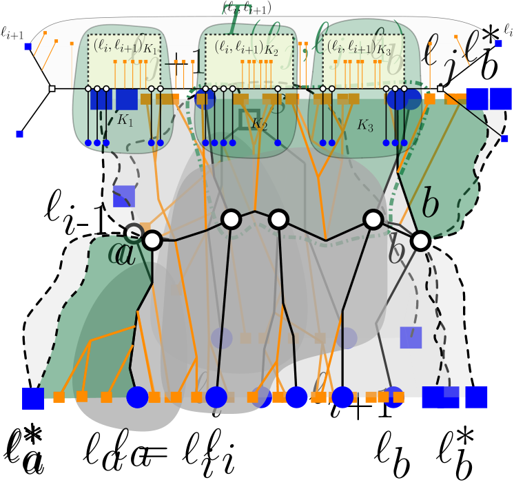
Figure 9: An interval $(\ell_{i},\ell_{i+1})$ related to three components $K_{1}$,$K_{2}$ and $K_{3}$. Interval $(\ell_{i},\ell_{i+1})$ is further subdivided into three intervals $(\ell_{i},\ell_{i+1})_{K_{1}}$,$(\ell_{i},\ell_{i+1})_{K_{2}}$ and $(\ell_{i},\ell_{i+1})_{K_{3}}$.

Proof.

Let $K$ be a component. The algorithm traverses the neighborhood of the representative leaf $\ell_{i}$ and takes a decision after at most $4z$, or $10z$, steps. In Lemma 5, we proved that if $\textnormal{{$nh$}}(\ell_{i})$ is confined, $\textnormal{{$nh$}}(\ell_{i})$ has at most $4\delta_{K}$, or $10\delta_{K}$, nodes. Hence, if $\delta_{K}\leq z$, the algorithm will succeed to select a marked leaf from $K$, because either $\textnormal{{$nh$}}(\ell_{i})$ is confined to $K$, and thus, the entire $\textnormal{{$nh$}}(\ell_{i})$ is traversed (lines 10-11,19-20), or else a delimiting node gets visited, and thus, the corresponding marked leaf is selected (lines 8-9,15-18). In all cases, we follow the proof of Lemma 2 and the neighborhood of the selected leaf is confined to $K$. Thus the selected leaf is among those counted in Lemma 3.

If on the other hand $\delta_{k}>z$, then the algorithm may fail to identify a marked leaf of $K$. We use the pigeonhole Lemma 4 to bound the number of these components. To this aim, we consider the set $I$ of all intervals induced by the marked leaves and the component of $\mathcal{T}$. For an interval $(\ell_{i},\ell_{i+1})$, which is not disjoint from $K$, let $(\ell_{i},\ell_{i+1})_{K}:=(\ell_{i},\ell_{i+1})\cap K$ denote its sub-interval of unmarked leaves that belong to$K$, see an example in Figure 9. Let $I_{z}$ be the intervals in $I$ that contain more than $z$ unmarked leaves. Then the algorithm may fail in at most $|{I_{z}}|$ components.

To bound $|{I_{z}}|$, we use Lemma 4 for $x=z=\left\lceil\frac{10c}{1-p}\right\rceil-1$. Then,

$$|I_{z}|\ \stackrel{{\scriptstyle(\ref{eq3})}}{{\leq}}\ \frac{cm}{z+1}\ =\ \frac{cm}{\left\lceil\frac{10c}{1-p}\right\rceil-1+1}\ \leq\ \displaystyle\frac{cm}{\frac{10c}{1-p}}\ =\ \frac{1-p}{10}m$$ (4)

Thus, the algorithm may fail for at most $\frac{1-p}{10}m$ components. By Lemma 1, there exist at least $\frac{1}{10}m$ components in $\mathcal{T}$, thus, the algorithm will succeed in selecting a marked leaf from at least

$$\frac{1}{10}m-|{I}_{z}|\ \stackrel{{\scriptstyle(\ref{eq4})}}{{\geq}}\ \frac{1}{10}m-\frac{1-p}{10}m\ =\ m\frac{p}{10}$$ (5)

components, concluding the proof. ∎

Lemma 7.

LABEL:algorithm has time complexity $O(\frac{1}{1-p}n)$.

Proof.

Labeling and partitioning the tree $\mathcal{T}$ into components can be done in $\Theta(n)$ time. Then, for each component the algorithm traverses a neighborhood performing at most $10z=\Theta(\frac{c}{1-p})$ steps. There are $\Theta(m)$ components, so we have $O(\frac{c}{1-p}\cdot m)$ time complexity. Recall that $c=\left\lceil\frac{r}{m}\right\rceil$. If $m=\Theta(n)$, then $c=\Theta(1)$, so $cm=\Theta(n)$. Else if $m=o(n)$, then $cm=\Theta(r)=\Theta(n)$. In all cases, the time complexity of the algorithm is $O(\frac{1}{1-p}n)$. ∎

By combining Lemmas 3, 6 and 7 we establish (and re-state) Theorem 2.

Theorem 2.

Let $\mathcal{T}$ be a marked tree of $n$ total leaves and $m$ marked leaves. Then there exist at least $\frac{1}{10}m$ leaves in $\mathcal{T}$ with pairwise disjoint neighborhoods such that no tree edge has its endpoints in two different neighborhoods. We can select at least a fraction $p$ of these $\frac{1}{10}m$ marked leaves in time $O(\frac{1}{1-p}n)$, for any $p\in(0,1)$.

If the parameter $p\in(0,1)$ is a constant, then the algorithm returns a constant fraction of the marked leaves and the time complexity of the algorithm is $O(n)$.

References

- [1] A. Aggarwal, L. Guibas, J. Saxe, and P. Shor. A linear-time algorithm for computing the Voronoi diagram of a convex polygon. Discrete & Computational Geometry, 4:591–604, 1989.
- [2] C. Bohler, R. Klein, A. Lingas, and C.-H. Liu. Forest-like abstract Voronoi diagrams in linear time. Computational Geometry, 68:134–145, 2018.
- [3] L. P. Chew. Building Voronoi diagrams for convex polygons in linear expected time. Technical report, Dartmouth College, Hanover, USA, 1990.
- [4] F. Chin, J. Snoeyink, and C. A. Wang. Finding the medial axis of a simple polygon in linear time. Discrete & Computational Geometry, 21(3):405–420, 1999.
- [5] K. Junginger, I. Mantas, and E. Papadopoulou. On selecting a fraction of leaves with disjoint neighborhoods in a plane tree. Discrete Applied Mathematics, 319:141–148, 2022.
- [6] K. Junginger and E. Papadopoulou. Deletion in abstract Voronoi diagrams in expected linear time and related problems. arXiv preprint arXiv:1803.05372, 2018.
- [7] E. Khramtcova and E. Papadopoulou. An expected linear-time algorithm for the farthest-segment Voronoi diagram. arXiv preprint arXiv:1411.2816, 2017.
- [8] R. Klein and A. Lingas. Hamiltonian abstract Voronoi diagrams in linear time. In Proceedings of the 5th International Symposium on Algorithms and Computation (ISAAC 1994), pages 11–19. Springer, 1994.
- [9] D.-T. Lee. On k-nearest neighbor Voronoi diagrams in the plane. IEEE transactions on computers, 100(6):478–487, 1982.
- [10] A. M.-C. So and Y. Ye. On solving coverage problems in a wireless sensor network using Voronoi diagrams. In Proceedings of the 1st Workshop on Internet and Network Economics (WINE 2005), pages 584–593. Springer, 2005.