11email: {fhinder,vvaquet,bhammer}@techfak.uni-bielefeld.de
A Remark on Concept Drift for Dependent Data††thanks: Funding in the frame of the ERC Synergy Grant “Water-Futures” No. 951424 is gratefully acknowledged.
Abstract
Concept drift, i.e., the change of the data generating distribution, can render machine learning models inaccurate. Several works address the phenomenon of concept drift in the streaming context usually assuming that consecutive data points are independent of each other. To generalize to dependent data, many authors link the notion of concept drift to time series. In this work, we show that the temporal dependencies are strongly influencing the sampling process. Thus, the used definitions need major modifications. In particular, we show that the notion of stationarity is not suited for this setup and discuss alternatives. We demonstrate that these alternative formal notions describe the observable learning behavior in numerical experiments.
Keywords:
Concept Drift Dependent Data Concept Drift Detection.1 Introduction
The world surrounding us is subject to constant change, which affects the increasing amount of data collected over time. As those changes, referred to as concept drift or drift for shorthand [gama2014survey], constitute a major issue in many applications, considerable research is focusing on this phenomenon. While in some applications, the goal is keeping an accurate model in the presence of drifts (stream or online leaning) [DBLP:journals/cim/DitzlerRAP15], in monitoring setups the goal is detecting and gathering information about the drift to inform appropriate reactions [OneOrTwoThings].
Frequently, the general assumption is that independent observations are collected over time even if they arrive in direct succession [DBLP:journals/cim/DitzlerRAP15, OneOrTwoThings]. However, in many real-world scenarios, temporal dependencies in the data have to be expected. This is for example the case when considering time series [lim2021time, aminikhanghahi2017survey, shalev2014understanding]. In this setting, the absence of change across multiple time series is described by the concept of stationarity. This notion is relevant if the goal is to obtain knowledge about the time series-generating process. This does not align with the goal of machine learning and monitoring, where we want to keep an up-to-date model based on our observations or detect anomalous behavior therein. In particular, we typically observe only one time series rather than multiple instantiations of time series. In this work, we analyze the connection of drift and stationarity in settings relevant to machine learning applications. We propose the notion of consistency when dealing with streaming data which stems from one time series. Moreover, we demonstrate in experiments, that this formalization captures the intuitive notion of drift for possibly dependent data streams.
This paper is organized as follows: In section 2 we recap the concept of drift and stochastic processes used later on. We categorize the possible setups and analyze them with respect to their convergence properties (section 2.3). In section 3, we provide examples showcasing that stationarity and drift do not align in settings of interest for machine learning (section 3.1). Thus, we propose the notion of consistency when dealing with a data stream possibly subject to time dependencies (section 3.2). We derive a first method checking for this concept (section 3.3). Finally, we confirm the theoretical arguments with numerical experiments (section 4) and conclude the work (section 5).
2 Problem Setup
In this work, we consider the problem of stream learning, i.e., at every given time point the data observed until , i.e., , is available. The observations can be independent of each other, dependent on the past (time series), or the time point of observation (drift). Depending on the specific setup, learning faces different problems, e.g., model adaption. In the following, we first give a precise formal definition of the notion of drift (of independent data) and stochastic processes/time series. We then discuss the challenges of defining drift for dependent data.
2.1 A Probability Theoretical Framework for Concept Drift
In the classical setup, machine learning assumes a time-invariant distribution on the data space and data points as i.i.d. samples drawn from it. This assumption is violated in many real-world applications, in particular, when learning on data streams. As a consequence, machine learning models can become inaccurate over time. As a first step to tackle this issue, we incorporate time into our considerations. To do so, let be an index set representing time and a (potentially different) distribution for every . Drift refers to the phenomenon that those distributions differ for different points in time [gama2014survey]. It is possible to extend this setup to a general statistical interdependence of data and time via a distribution on which decomposes into a distribution on and the conditional distributions on [DAWIDD, OneOrTwoThings]. One of the key findings of [DAWIDD] is a unique characterization of the presence of drift by the property of statistical dependency of time and data .
Definition 1.
Let be countably generated measurable spaces. Let be a drift process [DAWIDD] during on , i.e., a distribution on and Markov kernel from to . A time window is a non-null set. A sample (of size ) is an -tuple with i.i.d. We say that has drift if the probability of observing two different distributions in one sample is larger 0, i.e., .
Considerable work focuses on independent data streams with drift: Many authors consider the model accuracy as a proxy for drift and update the model if a decline in the accuracy is observed [DBLP:journals/cim/DitzlerRAP15]. As the connection between model loss and drift in the data generating distribution is rather lose [hinder2023hardness, ida2023], relying on distribution-based drift detection schemes instead of model loss-based schemes enables reliable monitoring [OneOrTwoThings]. Assuming independent data points , allows applying tools from classical statistics or learning theory [DAWIDD, ida2023]. In contrast, given temporal dependencies in the observed data, these strategies cannot be used successfully.
2.2 Stochastic Processes
Instead of drift processes, dependent data streams or time series can be modeled by stochastic processes [borodin2017stochastic]:
Definition 2.
Let be a probability space, a measurable space, and an index-set. A -valued stochastic process over is a map such that is a -valued random variable for all . We call the maps the paths of . For a finite, enumerated subset we refer to a realization of restricted to as a time series, i.e., where . The process is called stationary iff the distribution of is time invariant, i.e., for all . For we call a change point iff the distribution changes at . Assuming is a measurable space, we call measurable iff is measurable with respect to .
A measurable stochastic process is a random variable that takes values in the space of measurable functions from to . In particular, measurability is required if we want to integrate along the path as done in ergodic processes.
The main difference between stochastic and drift processes is that a stochastic process has one value for every point in time whereas a drift process yields a distribution. For example: Measuring the temperature of an object over time is a stochastic process because we read exactly one value. In contrast, a stream of ballots should be considered a drift process because the distribution is more interesting than a single vote.
2.3 A taxonomy of change detection in data streams
Different setups can be considered in the context of concept drift and dependent data. Intuitively, the absence of stationarity is the same as the presence of drift. We investigate this relationship in more detail: We first propose a categorization of the possible setups as visualized in fig. 1. In the remainder of this section, we describe the different setups.
Independent data points
The classical setup of concept drift states that we have several independent data points that are sampled from potentially different distributions. This can be investigated for general machine learning [gama2014survey, DBLP:journals/cim/DitzlerRAP15, ida2023] or for drift detection [DAWIDD, MMD, KCpD, KFRD, OneOrTwoThings]. As we can characterize a drift process solely by the values of all functions integrated over all time windows [DAWIDD, hinder2023hardness] we can test for drift as follows: instead of only tracking the data points we additionally consider the time of observation, . Using this information we can compute the value
| -a.s. | (1) | ||||
where is the random-event. In particular, the limit always applies, and the value on the right-hand side does not depend on only on the drift process (and and ). This justifies defining drift as being observed with a probability larger than zero. Thus, in an independent data stream, the presence drift is the same as the absence of stationarity (up to a null set).
Multiple (independent) streams
In real-world applications, data points frequently are not independent. Instead of observing an independent data stream, we observe one or multiple stochastic processes. Let us consider the case of multiple ones first: Let be sampled independently from the same distribution and each modeling the temporal dependency of consecutive observations. This setup can be reduced to the independent data streams as above:
Theorem 2.1.
Let and be countably generated, e.g., . Let i.i.d. measurable stochastic processes and any probability measure on . Let be i.i.d. and denote by . Then all are i.i.d. and for all , i.e., they form a sample of the drift process .
Furthermore, has drift (in the sense of definition 1) if and only if there exists a null-set such that restricted onto is stationary.
Proof.
As is measurable, so is the graph map as for we have . And it suffices to check this on a generator. Applying this map twice, we have
is measurable. For measurable we have
where denotes the conditional expectation function given in the sense. Thus, .
Notice that is a -valued random variable. Let be finite and w.l.o.g. . Let time windows, . Consider
Thus, are indeed i.i.d. with .
If is stationary, then for all thus is a null-set so there is no drift. Conversely, assuming there is no drift then using the ideas of [DAWIDD] there exists such that for -a.s. all and thus for all for some -null set . ∎
Thus, we consider the case of a single dependent path which is the standard setting for time series analysis [truong2020selective, aminikhanghahi2017survey] in the following.
Ergodicity and mixing
Considering only one dependent process we first encounter a phenomenon that we refer to as the uncertainty principle of drift learning. To understand this assume we want to estimate the value of . As the probability of making an observation exactly at time is zero, we replace it with a small time window . In the independent setup, we simply sample more and more data points and gain better and better estimation (see eq. 1) and then successively shrink towards . However, in the single-path setup, we can only sample one path at several time points. As a consequence, the inner integral on the right-hand side of eq. 1 becomes a time-average:
As can be seen, the right-hand side now does depend on and does not necessarily converge to the mean of the underlying distribution during also known as space average, i.e., . Intuitively speaking, dependency limits the amount of local information and due to drift, we cannot obtain more information by considering larger time windows. The special cases in which the convergence holds are summarized in fig. 2 and discussed in the following.
Processes for which such convergence holds are referred to as ergodic processes [borodin2017stochastic]. They allow precise estimations and learning under the assumption of stationarity [adams2010uniform]. Yet, they have arbitrarily slow convergence [krengel1978speed]. A common property used to counteract this issue is offered by mixing processes that impose a rate on becoming independent. This leads to uniform convergence similar to the independent case and has been used by several authors to prove statements on learnability in the stationary [yu1994rates, kontorovich2007measure] and non-stationary setup [hanneke2019statistical, agarwal2012generalization].
Yet, both ergodic and mixing processes usually require infinite temporal horizons to achieve convergence. As we are usually concerned with limited time the results might be interesting from a theoretical point of view but have little practical relevance. Also, due to the uncertainty principle we introduced before most make additional requirements that limit the non-stationarity in one way or another. In particular, its relation to drift detection in the monitoring setup is not clear.
Not-ergodic processes
Ergodicity usually describes that the time average equals the space average for infinitely large time windows. We will call processes for which there are either no time windows for which equality holds or for which this cannot be predicted not-ergodic.
It is obvious that stationarity is not a reasonable tool to discuss not-ergodic processes as there is no real connection to the underlying distributions. This implies that there cannot be any formal guarantees regarding generalization properties in the usual sense.
Research questions
Based on the presented analysis we notice that there do exist theoretical results on detecting drift in dependent data but their relevance for practical setups is questionable. This leads us to the following questions that we address in the following:
-
1.
Is non-stationarity a suitable definition for the notion of concept drift for dependent data?
-
2.
Does there exist an alternative notion that is more suitable for practical application (this includes testability on finite temporal horizons)?
3 Consistency Property
In this section, we investigate the suitability of stationarity to model the equivalent of drift as used for independent data streams on time series. First, we provide (counter-)examples that show that this is not the case. Based thereon, we derive the concept of temporal consistency to formalize drift for time series. Finally, we derive a method to test consistency.
3.1 Drift is not Non-Stationarity
That the presence of drift is not the same as the absence of stationarity for dependent data streams can be shown by the following, simple counterintuitive examples:
Example 1.
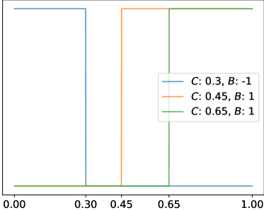
Let and and independent random variables with for , and . Consider the process whose paths take values in and switch sign exactly once (see fig. 3). Then we have and therefore is stationary if and only if and otherwise every is a change point. Yet, every path has exactly one jump at time .
Proof.
Notice that and for all by definition. Hence, and for all . Therefore, for all . By considering we see that stationarity holds if and only if ∎
Example 2.
Consider a teacher student scenario: Let . Let and where is the teacher weight vector which is independently resampled every time steps, i.e., . Then is a labeled data stream that is -mixing and stationary. Yet, every time steps the teacher is changed in a completely random way.
Proof.
Since we have
Thus, for all and we have so the process is -mixing. Now, since and the right-hand side does not depend on the process is stationary. ∎
Both examples show a common theme: If we consider one path only then there are obvious changes, but if we average over several paths then those changes even out (at least for ). Thus, we can conclude that in contrast to stationarity, drift is a path-wise notion. A naïve way to solve this problem is to apply the definition of stationarity path-wise, i.e., . However, such processes are essentially constant. Therefore the notion is far too restrictive to be of interest:
Lemma 1.
Let and be countably generated with having a measurable diagonal, i.e., . Let be a measurable stochastic process and a measure on with independent of each other and . It holds -a.s., i.e., , if and only if is constant for -a.e. , i.e., there exists a random variable such that .
Proof.
Due to the measurability of the equality sets are measurable.
Assuming exists, then we have
where holds because and
Otherwise, define . Since is measurable and is a probability measure is a Markov kernel. Yet, since for all we have and therefore for all we have thus so
by Jensen’s inequality and Fubini’s theorem. Thus, -a.s. so there exists a null set such that for all . Since is countably generated is a Dirac-measure for every . Thus, there exists a set theoretical map such that for all and for all . Yet, since is measurable the mapping must be measurable for all and thus is measurable as also . Hence, is a -value random variable and by construction and thus -a.s. ∎
Thus, equality is far too restrictive for dependent data. Yet, the definition of drift as “a change of the distribution over time” stems from the batch setup with independent data where we do not expect any change and are able to make arbitrarily precise measurements as discussed in section 2.3. If we expect some kind of temporal dynamics, like seasonality, it might be better to rephrase this as “the distribution changes in an unexpected way” where “unexpected” means “in a way our model cannot cope with without retraining”. This is a more suitable description as shown in the following example:
Example 3.
Let . For consider the family of stochastic processes with uniformly distributed. Then is the only stationary process in this family. Yet, given two points we can estimate from correctly with probability 1.
Proof.
Observe that and . Stationarity in particular implies constant expectation. Therefore, is the only solution that can admit a stationary process. Yet, for we have where ! holds since has period . Hence, is stationary.
Observe that for all we have . Thus, once we know there are at most two choices left for . Yet, the chance of is 0 and in every other case we can determine uniquely. ∎
In the next section, we explore the idea of “unexpected change” in more detail, leading to our substitute for the notion of stationarity.
3.2 Temporal Consistency
In the last section, we discussed that stationarity is a sub-optimal choice to describe the notion of drift in a dependent setup, rather we should look for “unexpected changes of a single stream”. We will now formalize the idea, referring to the new notion as consistency. Formally, we define a collection of functions that assign a loss to the paths. Consistency then refers to time-invariant losses.
Definition 3.
Let be a probability measure on . Let be a collection of measurable functions from to . A path is consistent with respect to iff and equality holds for
where are all finite disjoint coverings of by time windows.
Consistency can be used to check whether belongs to a predefined function class but also generalizes the notion of model drift as considered by [hinder2023hardness] and is closely connected to -model drift [ida2023]:
Lemma 2.
Let and . Let be a colleciton of measurable functions from to and a hypothesis class with loss on . It holds:
-
1.
Consider then is -consistent if and only if in the -sense.
-
2.
Consider and assume that the functions in are continuous, and that for all up to a -null set the closure of the images of under contain , i.e., for all and there exists a such that , then can be approximated in by cadlag function piecewise contained in . In particular, is -consistent if and only if where the closure is taken in the -sense.
-
3.
Consider then is not -consistent implies that the drift process has -model drift [ida2023].
Proof.
1) if on a non-null set then not consistent, otherwise -a.s.
2) We show that we can approximate by functions piecewise contained in . To do so we first show that we can approximate by piecewise constant, cadlag functions with values in and then that a constant function can be approximated by a cadlag function that is picewise contained in .
Let and be some point such that for some . Such a point exists as we can approximate by a continuous function with values in all of which is bounded since is compact, this implies the existence by use of the triangle inequality. Since is polish, is a tight measure and thus there exists a compact set such that and by Heine-Borel we may assume for some . Define and
The set is an open cover of and thus admits a finite sub-cover with associated points . Let the pre-images of under (notice that the pre-image of is empty). Since is polish, is regular and thus there exist open sets such that and then denoting we have
where holds for because where the first inequality is Hölder’s inequality with applied to the indicator function, for we have so , and holds by a similar application of Hölder’s inequality. Thus, any piecewise constant function with is a good approximation of . To construct consider the open covering of . This is a cover indeed, as every is contained in some . Choose a finite sub-cover and points such that for all there is a and thus a such that . By construction we have that if then also and we can hence obtain an approximation of by a picewise constant, cadlag function. Hence, if we can approximate constant functions by functions in we are done.
Let and assume is constant. Denote by and extend all function in by a constant onto all of . Consider . Notice that every is contained in some ball in as by assumption there exists a such that and thus for some as it is the pre-image of an open set under a continuous function.
Fixate a function . Since is compact is bounded and thus . Furthermore, as is polish, is regular and thus there exists an open set such that . Define . Notice that every is contained in some ball in so in particular every is contained in some ball in .
Hence, is an open cover of which admits a finite sub-cover as is compact. Thus, there exists a sequence such that with . For every with we have that as we halved the radii, so by choosing for all those the error is still below . Similarly, for every with there is a function associated with it such that as we halved the radii. Combining all the pieces we obtain the desired function.
3) Assuming the left-hand side is strictly smaller than the right-hand side. Then there has to exist a and for which strict inequality already holds. Let us assume that is minimal, then all have to be different as otherwise we could use which is smaller. On the other hand, it holds as otherwise both sides have to be equal. Thus there have to exist at least two disjoint windows and with and analogous for . By definition of and minimality of this implies -model drift using that . ∎
Thus, we define which functions are consistent. In the next section, we derive an algorithm that checks for consistency for just this setup.
3.3 Measuring Consistency of a Noisy Stochastic Processes
To apply consistency, we show how to check whether a stochastic process is essentially contained in a predefined function class comparable to lemma 2.2. We consider a noisy (measured) version of the function , i.e., where is an independent noise process, and we want to check whether . To do so we use a newly designed loss that can compensate for the noise. We assume that specifies global phenomena, e.g., linear, polynomial, or exponential trends, periodicity, etc. Thus, contains no local phenomena.
An algorithmic solution is then given by the following: We fit a model to and then check whether does contain any structure using a local model like -NN. If this is not the case, i.e., the local model is not better than random chance, then .
In case the paths are equidistantly sampled, the -NN simplifies to the following loss which has the desired properties.
Theorem 3.1.
Let with sampling time points . Let such that and odd, denote by . Let be measurable maps and with and denote by the subsample according to . We define the -local MSE as:
If , , and are bounded, then it holds
And, if and as then the -local MSE of the empirical process converges in probability to the MSE of the true signal as .
Proof.
We have
Since the second term vanishes and the first term equals
using that all are independent. By reordering we see that occurs at most times, thus, the first term is bounded by
Similarly, by Jensen’s inequality the third term is bounded by the MSE using the same reordering where we have to add at most terms in case each bounded by . Hence, we have
Together with the other bound we thus obtain
and we arrive at the statement by taking absolute values.
Under the assumptions on we have that , as the first term goes to 0 and the second to 1 so the product converges to 0 and therefore . Furthermore, denoting by an upper bound of all and using we can bound
so the expectation of the local -MSE converges to the MSE of the original signal as .
To show that the empirical local -MSE converges to its expectation, we show that the variance tends to 0 as . To do so, first observe that if are random variables with , then
Thus, by identifying we see that it remains to show that as .
By writing
we see by using that is suffices to consider
and with an upper bound of we have
where holds because every term for all and any. So . ∎
The -local MSE is essentially the usual MSE except that smoothing is applied to the training data and the model. Indeed, for linear models with non-linear preprocessing, this allows for efficient training. Yet, in our experiments, training with the usual MSE usually leads to better results and the local MSE is only used for testing.
In the next section, we empirically evaluate the different methods to probe consistency. We also check the validity of the arguments presented in section 3.1 using numerical evidence.
4 Numerical Evaluation
We perform numerical evaluations on artificial data to confirm the presented theory experimentally.111The experimental code as well as all datasets can be found at https://github.com/FabianHinder/Remark-on-Dependent-Drift.
4.1 Testing Stationarity
We start by verifying that stream learning algorithms indeed operate path-wise and thus are not well described using the notion of stationary. To do so we generate paths according to the distribution in example 1 and example 3 in a stationary and non-stationary case. We then apply the Kernel Change-point Detector [KCpD] (KCpD) to the resulting paths. In the case of example 1 the detector determines the value of (the moment of the jump) with less than 2 samples offset each time, independent of whether the distribution was stationary or not. Similarly, for example 3 every point is considered a change point. Furthermore, using the sub-sampling process described in theorem 2.1 the detector alerts a drift if and only if the initial distribution is not stationary, as predicted by the theorem. We also applied the Augmented Dickey-Fuller [ADF] (ADF), and the Kwiatkowski-Phillips-Schmidt-Shin [KPSS] (KPSS) test which are used to test for stationarity in time series to the data. The resulting -values do not differ for the stationary and non-stationary cases for both tests. We thus conclude that the methods do not check for the stationarity of the underlying distribution or rather fail to do so but rather for properties of the single path.
4.2 Evaluation of Method
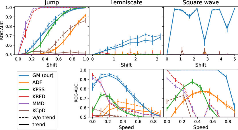
To evaluate how well existing methods can deal with consistency we consider the following synthetic datasets: “Jump” similar to example 1, “Lemniscate” , and “Square wave” where is given by a square wave. In all cases, we added normal distributed noise and considered a version with an additive linear trend (which is not considered as drift). Drift is induced in the middle of the path. In the case of Jump a jump in the mean value is introduced, for Lemniscate and Square wave we either added a shift in time, i.e., for , for , or slowed down time, i.e., for , for . All with different intensities. We considered ADF, KPSS, and KCpD as well as MMD [MMD] and KFRD [KFRD] as methods from the literature, where the latter two are provided with the correct change point candidate. ADF and KPSS performed trend corrections. For KCpD we used the number of found change points, for all other methods the returned -value.222We also considered auto-regressive models based on Ridge and -NN regression but found them to only work on the Jump dataset. As suggested by theorem 3.1, we use the lMSE as an indicator for non-consistency using a linear model with (trig-)polynomial (up to degree 15) as preprocessing (GM). For every setup, we performed 1,000 independent runs and evaluated the obtained scores using the ROC-AUC to measure how well the methods separate the drifting and non-drifting paths [hinder2022suitability]. The results are presented in fig. 4.
As can be seen, the classical drift detectors KCpD, MMD, and KFRD only work for Jump without trend and in case of an extreme slow down, although KCpD and KFRD were explicitly designed for time series data [KCpD, KFRD]. The other methods are less affected by the trend. ADF and KPSS perform quite well on Jump and in the cases of slow down. However, none of the methods from the literature can deal with a time shift on any dataset. Our method performs quite well on all datasets. In particular, it is the only one that can deal with time shifts.
5 Conclusion
In this work, we argued that drift and stationarity do not align in many setups realistic for online learning and monitoring of dependent data. Next to providing theoretical counter-examples, we ran a numerical evaluation confirming our considerations. Besides, we proposed the concept of consistency which is more suitable to the tasks at hand.
Yet, it is still unclear how problematic the discrepancy between stationarity and drift is. Also, besides the notion of (strict) stationarity we studied in this paper, the notion of wide-sens stationarity might offer a well-suited choice for some cases. An in-depth investigation of this seems interesting. Furthermore, so far we have only considered the notion of consistency for stochastic processes. A description of the phenomenon of dependent data streams by means of “dependent drift process” and a suited generalization of the notion of consistency are still outstanding.
Furthermore, the notion of consistency is very similar to the notion of model drift studied in [hinder2023hardness] who show that such approaches are not suited for monitoring tasks in the independent setting. Though we believe that this does not pose a problem as the proof is heavily founded on the independence assumption, considering this problem in detail appears to be very relevant.
References
- [1] Adams, T.M., Nobel, A.B.: Uniform convergence of vapnik–chervonenkis classes under ergodic sampling (2010)
- [2] Agarwal, A., Duchi, J.C.: The generalization ability of online algorithms for dependent data. IEEE Transactions on Information Theory 59(1), 573–587 (2012)
- [3] Aminikhanghahi, S., Cook, D.J.: A survey of methods for time series change point detection. Knowledge and information systems 51(2), 339–367 (2017)
- [4] Borodin, A.N.: Stochastic processes. Springer (2017)
- [5] Dickey, D., Fuller, W.: Distribution of the estimators for autoregressive time series with a unit root. JASA. Journal of the American Statistical Association 74 (06 1979). https://doi.org/10.2307/2286348
- [6] Ditzler, G., Roveri, M., Alippi, C., Polikar, R.: Learning in nonstationary environments: A survey. IEEE Comp. Int. Mag. 10(4) (2015)
- [7] Gama, J., Žliobaitė, I., Bifet, A., Pechenizkiy, M., Bouchachia, A.: A survey on concept drift adaptation. ACM computing surveys (CSUR) 46(4), 1–37 (2014)
- [8] Gretton, A., Borgwardt, K.M., Rasch, M.J., Schölkopf, B., Smola, A.J.: A kernel method for the two-sample-problem. In: NIPS. pp. 513–520 (2006)
- [9] Hanneke, S., Yang, L.: Statistical learning under nonstationary mixing processes. In: The 22nd International Conference on Artificial Intelligence and Statistics. pp. 1678–1686. PMLR (2019)
- [10] Harchaoui, Z., Cappé, O.: Retrospective mutiple change-point estimation with kernels. In: 2007 IEEE/SP 14th Workshop on Statistical Signal Processing. pp. 768–772. IEEE (2007)
- [11] Harchaoui, Z., Moulines, E., Bach, F.: Kernel change-point analysis. In: Koller, D., Schuurmans, D., Bengio, Y., Bottou, L. (eds.) NIPS. vol. 21. Curran Associates, Inc. (2008)
- [12] Hinder, F., Artelt, A., Hammer, B.: Towards non-parametric drift detection via dynamic adapting window independence drift detection (dawidd). In: International Conference on Machine Learning. pp. 4249–4259. PMLR (2020)
- [13] Hinder, F., Vaquet, V., Brinkrolf, J., Hammer, B.: On the change of decision boundary and loss in learning with concept drift. In: International Symposium on Intelligent Data Analysis. pp. 182–194. Springer (2023)
- [14] Hinder, F., Vaquet, V., Brinkrolf, J., Hammer, B.: On the hardness and necessity of supervised concept drift detection (2023)
- [15] Hinder, F., Vaquet, V., Hammer, B.: Suitability of different metric choices for concept drift detection. In: International Symposium on Intelligent Data Analysis. pp. 157–170. Springer (2022)
- [16] Hinder, F., Vaquet, V., Hammer, B.: One or two things we know about concept drift – a survey on monitoring evolving environments (2023)
- [17] Kontorovich, L.: Measure concentration of strongly mixing processes with applications. Carnegie Mellon University (2007)
- [18] Krengel, U.: On the speed of convergence in the ergodic theorem. Monatshefte für Mathematik 86(1), 3–6 (1978)
- [19] Kwiatkowski, D., Phillips, P.C., Schmidt, P., Shin, Y.: Testing the null hypothesis of stationarity against the alternative of a unit root: How sure are we that economic time series have a unit root? Journal of econometrics 54(1-3), 159–178 (1992)
- [20] Lim, B., Zohren, S.: Time-series forecasting with deep learning: a survey. Philosophical Transactions of the Royal Society A 379(2194), 20200209 (2021)
- [21] Shalev-Shwartz, S., Ben-David, S.: Understanding machine learning: From theory to algorithms. Cambridge university press (2014)
- [22] Truong, C., Oudre, L., Vayatis, N.: Selective review of offline change point detection methods. Signal Processing 167, 107299 (2020)
- [23] Yu, B.: Rates of convergence for empirical processes of stationary mixing sequences. The Annals of Probability pp. 94–116 (1994)